Estimation of the Quantum Fisher Information on a quantum processor

Abstract

The quantum Fisher information (QFI) is a fundamental quantity in quantum physics and is central to the field of quantum metrology. It certifies quantum states that have useful multipartite entanglement for enhanced metrological tasks. Thus far, only lower bounds with finite distance to the QFI have been measured on quantum devices. Here, we present the experimental measurement of a series of polynomial lower bounds that converge to the QFI, done on a quantum processor. We combine advanced methods of the randomized measurement toolbox to obtain estimators that are robust against drifting errors caused uniquely during the randomized measurement protocol. We estimate the QFI for Greenberger–Horne–Zeilinger states, observing genuine multipartite entanglement and the Heisenberg limit attained by our prepared state. Then, we prepare the ground state of the transverse field Ising model at the critical point using a variational circuit. We estimate its QFI and investigate the interplay between state optimization and noise induced by increasing the circuit depth.

The quantum Fisher information [1] exhibits profound connections with multipartite entanglement [2, 3, 4, 5] and plays a crucial role in various quantum phenomena, including quantum phase transitions [6, 7] and quantum Zeno dynamics [8]. It holds vast applications ranging from quantum metrology [9, 10, 11] and many-body physics [12, 13] to resource theory [14]. It is defined with respect to an Hermitian operator $A$ and a quantum state $\rho$, and can be expressed in the form [9]

$$F_{Q}=2\sum_{(\mu,\nu),\lambda_{\mu}+\lambda_{\nu}>0}\frac{(\lambda_{\mu}-\lambda_{\nu})^{2}}{\lambda_{\mu}+\lambda_{\nu}}|\bra{\mu}A\ket{\nu}|^{2},$$ (1)

in terms of the spectral decomposition $\rho=\sum_{\mu}\lambda_{\mu}\outerproduct{\mu}{\mu}$ of the state under consideration. The inverse of the QFI limits the estimation accuracy of an unknown parameter as given by the quantum Cramér-Rao bound [10, 9]. In parameter estimation, there exist quantum states that saturate the Cramér-Rao bound and provide metrological sensitivities beyond the shot-noise limit (or standard quantum limit) [11]. For $N$ qubits (as we will consider throughout this paper), with a collective spin operator $A=\frac{1}{2}\sum_{j=1}^{N}\sigma_{j}^{(\tau)}$ , entangled quantum states that provide enhanced sensitivities for metrological tasks satisfy $F_{Q}>N$ [11]. Multipartite entanglement can be certified via QFI in terms of $k$-producibility of the state $\rho$, i.e. a decomposition into a statistical mixture of tensor products of $k$-particle states. In particular, the inequality $F_{Q}>\Gamma(N,k)$, with $\Gamma(N,k)=\left\lfloor\frac{N}{k}\right\rfloor k^{2}+\big{(}N-\left\lfloor\frac{N}{k}\right\rfloor k\big{)}^{2}$, implies that a state is not $k$-producible, i.e that it has an ‘entanglement depth’ of at least $k+1$ [2, 3] and is said to be $(k+1)$-partite entangled. An $N$-qubit state with an entanglement depth of $k=N$ is called genuinely multipartite entangled (GME).

Identifying experimental methods to extract the QFI of arbitrary quantum states is an outstanding challenge and is a current topic of interest. One way to calculate the QFI corresponds to performing quantum state tomography to access the eigenvalues and the eigenstates of $\rho$ in order to evaluate Eq. (1). This approach necessitates an expensive measurement budget [16, 17, 18], and is thus limited to small system sizes. In the specific case when the quantum state is a thermal state, the QFI can be measured directly using dynamical susceptibilities [6]. Alternatively, many lower bounds to the QFI have been proposed and measured such as spin-squeezing inequalities expressed as expectation values of linear observables [19, 20, 21, 22, 23, 24, 25, 26] and also non-linear quantities as a function of the density matrix [27, 28, 29, 30, 31, 32]. For a thorough account of them we refer the reader to [33] and references therein.

In this work, we estimate the QFI expressed in terms of a converging series of polynomials of order $n$ in the density matrix $\rho$ [34], for a state prepared on the 33-qubit IBM superconducting device ‘ibm_prague’ equipped with an ‘Egret r1’ quantum processor [35]. We realise a robust protocol, employing the randomized measurement toolbox, to measure these polynomials [36] and tame the drifting gate and readout errors that particularly affect the randomized measurement protocol during the full course of the experiment. We measure the QFI for two prototypical examples of states: (i) the Greenberger–Horne–Zeilinger (GHZ) state and (ii) the ground state of the transverse field Ising model (TFIM) at the critical point [37].

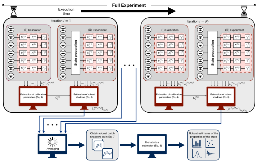
Figure 1: Overview of experimental protocol (Sec. I) and post-processing (Sec. II). The experimental protocol is comprised of several ‘iterations’ $i=1,\dots,N_{I}$. Each of them consists of a calibration step (i) and the experiment on the state of interest $\rho$ (ii). From the unitaries and bit-strings recorded in (i) we estimate the noise parameter $G_{j}^{(i)}$ (Eq. (4)), that is used for the construction of the robust shadows $\tilde{\rho}^{(r_{i},m_{i})}$ (Eq. (3)) together with the data from step (ii). All robust shadows are then collected and averaged in batches to obtain $b=1,\dots,N_{B}$ robust batch shadows $\hat{\rho}^{(b)}$ (Eq. (7)). These are used for computing the multi-copy observables of interest through the U-statistics estimator (Eq. (8)). Our experiments are performed on the IBM superconducting qubit device ‘ibm_prague’ [35].

Remarkably, our approach is not restricted to the QFI and to the states presented here. It provides robust and unbiased estimators for any arbitrary non-linear multi-copy functionals of a density matrix $\rho$.

The paper is organised as follows. We first describe in detail the experimental setting and the necessary steps for collecting the data for the estimation of the QFI (Sec. I), as sketched in Fig. 1. Then, we elaborate on the post-processing methods and their efficiency in terms of measurement budget and noise mitigation (Sec. II). Finally we discuss the experimental results (Sec. III) and draw our conclusions.

Additionally, we provide more details on our work in the Appendices, organised as follows. In App. A we give the expression of the QFI and of its lower bounds in terms of polynomials of $\rho$ as in Eq. (1). In App. B we provide the analytical details of our post-processing protocol and an experimental analysis of the noise mitigation parameters we employ. In App. C we investigate the noise in the platform. In App. D we introduce an estimator to verify the locality of the noise and estimate it for the our experimental setup. In App. E we provide more results for both the experiments discussed in the main text. Finally, in App. F we perform numerical investigation on the statistical error of our estimator for justifying the choice of the parameters used in our experiment.

I Data Acquisition with randomized measurements

Our approach, illustrated in Fig. 1, harnesses the capabilities of the randomized measurement toolbox and is comprised of several repetitions of two building blocks: (i) Calibration of randomized measurements and (ii) randomized measurements on the state of interest $\rho$. The calibration step depicted in Fig. 1(i) is employed to learn and mitigate the gate and readout errors that affect the measurements, as described in Refs. [38, 39]. This relies on the ability of the experimental platform to prepare a specific state with high fidelity. In this work, we fix the calibration state to be $\ket{\mathbf{0}}\equiv\ket{0}^{\otimes N}$, which is reproducible with high efficiency on our quantum processor. The data collected in step (ii) are then used for estimating the observables we are interested in. We call each run of (i) and (ii) an ‘iteration’ of the experiment. Performing consecutive iterations allows to account for the temporal variations in gate and readout errors. Assuming that the temporal fluctuations of the errors affecting the randomized measurements protocol for each iteration is negligible, each calibration step captures the specific error profile of a distinct time window within the overall experimental run. We demonstrate experimentally the fluctuation of the noise in App. C.1.

First, let us start by recalling how the randomized measurement protocol works on a state $\rho$ in the absence of noise. We begin by preparing the $N$-qubit quantum state $\rho$. Then we apply local random unitaries $U=U_{1}\otimes\dots\otimes U_{N}$ that are sampled from the circular unitary ensemble [40]. The rotated state $U\rho U^{\dagger}$ is then projected onto a computational basis state $\ket{\mathbf{s}}=\ket{s_{1},\dots,s_{N}}$ by performing a measurement. To make the protocol robust against the noise occurring in the quantum device, we apply the measurement sequence described above on the states $\ket{\mathbf{0}},\,\rho$ in steps (i),(ii) of Fig. 1, respectively. As described before, the data collected from (i) is used to mitigate the errors induced by the noisy measurement protocol in step (ii) [38, 39].

Measurement budget

The full experiment is divided in a total of $N_{I}$ iterations (labeled by $i=1,\dots,N_{I}$). For steps (i) and (ii) in each iteration $i$, we apply the same $N_{U}=200$ local random unitaries $U^{(r_{i})}=U_{1}^{(r_{i})}\otimes\dots\otimes U_{N}^{(r_{i})}$, with $r_{i}=1,\dots,N_{U}$ , and (for each unitary) record $N_{M}=1000$ measurement outcome bit-strings $\mathbf{s}^{(r_{i},m_{i})}=(s^{(r_{i},m_{i})}_{1},\dots,s^{(r_{i},m_{i})}_{N})$ with $m_{i}=1,\dots,N_{M}$.

The total measurement budget ($N_{I}N_{U}N_{M}$) that is required to reach a given accuracy for an estimator depends on the size of the system $N$ [36]. In particular, for our experiments we employ a total of $N_{U}^{\textrm{tot}}=N_{I}N_{U}=300\cdot 2^{0.5N}$ unitaries in order to obtain an estimation error of $\sim 10\%$ on the highest-order estimated lower bound of the QFI. Note that the higher the order, the more measurements are needed to overcome statistical fluctuations. Numerical investigations on the measurement budget are detailed in App. F.2.

II Estimation of the QFI from randomized measurement data

In this section we explain all the steps we employ for postprocessing the data obtained from the randomized measurement protocol.

II.1 The QFI as a converging series of polynomials

The data we collect during the execution of our protocol can be used to faithfully estimate quantum state properties via the randomized measurements toolbox [36]. While the QFI $F_{Q}$, as written in Eq. (1), cannot be accessed directly by randomized measurements, it can be alternatively expressed and estimated in terms of a converging series of monotonically increasing lower bounds $F_{n}$ [34]. For the first three orders $n=0,\,1,\,2$, one can write explicitly

$$F_{0} =4\,\mathrm{Tr}(\rho\big{[}\rho,A\big{]}A)\,,$$

$$F_{1} =2\,F_{0}-4\,\Tr(\rho^{2}[\rho,A]A)\,,$$ (2)

$$F_{2} =3(F_{1}-F_{0})+4\,\Tr(\rho^{2}[\rho^{2},A]A)\,,$$

where $[\cdot,\cdot]$ is the commutator. In our work, the observable under consideration is taken to be $A=\frac{1}{2}\sum_{j}\sigma_{j}^{z}$, where $\sigma_{j}^{z}$ is the Pauli-$z$ operator acting on qubit $j$. We provide the general expression for $F_{n}$ in App. A.

Each function $F_{n}$ is a polynomial function of the density matrix (of order $n+2$); such functions can be accessed via randomized measurements, as it has been shown for entropies [42, 43, 44, 45, 46, 47], negativities [48, 49, 50], state overlaps [51, 52, 53], scrambling [54] and topological invariants [55, 56]. Note that with the randomized measurement protocol, one can also characterize entanglement based on statistical correlation between measurement outcomes as reviewed in Ref. [57]. With respect to previous applications, here we mitigate the noise in the measurement protocol to extract reliable estimation from the noisy measurements on the quantum device, using the technique presented in Refs. [38, 39]. We will show that this step is necessary for faithfully estimating the QFI for a number of qubits $N\gtrsim 8$.

II.2 Assumptions on the noise model for the post-processing step

The basic assumptions on the noise model for our post-processing protocol are as follows. As in Ref. [38], we consider a gate-independent noise channel $\Lambda$, applied after the random unitaries: that is, for each chosen $U$ the state $\rho$ transforms as $\Lambda(U\rho U^{\dagger})$. We assume that the noise channel $\Lambda$ is constant during each iteration $i$ – we label it as $\Lambda^{(i)}$ – and may change between each iteration. We provide experimental evidence of the variation of the noise over different iterations – that is remarkably captured by our protocol – in App. C.1 . Additionally, we assume the noise to be local for each qubit, so that $\Lambda^{(i)}=\Lambda^{(i)}_{1}\otimes\dots\otimes\Lambda^{(i)}_{N}$. In App. D we provide and implement a method to verify the assumption of locality of the noise, based on the calibration data. Additionally, in App. E.3, we show that tracking the variation of the noise over the different iterations is essential to provide faithful estimations of the QFI.

II.3 Robust shadows estimation

The first step towards the measurement of the QFI is to construct estimators of the density matrix $\rho$ from noisy measurements. This object, called a ‘robust shadow’ [38], can be defined as

$$\tilde{\rho}^{(r_{i},m_{i})}$$

$$\!=\bigotimes_{j=1}^{N}\!\left(\!\alpha^{(i)}_{j}\,{U_{j}^{(r_{i})}}^{{\dagger}}\!\outerproduct{s_{j}^{(r_{i},m_{i})}}{s_{j}^{(r_{i},m_{i})}}\!{U_{j}^{(r_{i})}}+\beta^{(i)}_{j}\mathbb{1}\!\right)\!,$$ (3)

where $\alpha^{(i)}_{j}=\frac{3}{2G^{(i)}_{j}-1}$ and $\beta^{(i)}_{j}=\frac{G^{(i)}_{j}-2}{2G^{(i)}_{j}-1}$. Here $r_{i}$ labels a unitary in iteration $i$ and $m_{i}$ labels a measured bit-string after the application of $U_{j}^{(r_{i})}$. The quantity in Eq. (3) satisfies $\mathbb{E}[\tilde{\rho}^{(r_{i},m_{i})}]=\rho$, where the average is taken over the applied unitaries and measurements. This equality is necessary to derive the unbiased estimators of the lower bounds $F_{n}$ [34].

The quantity $G^{(i)}_{j}$ contains the relevant information on the noise induced (on qubit $j$, in iteration $i$) during the measurement protocol. It is defined as

$$G^{(i)}_{j}=\frac{1}{2}\sum_{s_{j}=0,1}\bra{s_{j}}\Lambda^{(i)}_{j}(\outerproduct{s_{j}}{s_{j}})\ket{s_{j}}$$ (4)

and can be interpreted as the average ‘survival probability’ of the two basis states of qubit $j$. In the absence of noise, $G^{(i)}_{j}=1$ ($\forall\;j=1,\dots,N$), and one recovers the standard ‘classical shadow’ [58]. In the opposite limit of fully depolarising noise, $G^{(i)}_{j}=1/2$, the coefficient $\alpha^{(i)}_{j},\beta^{(i)}_{j}$ diverge and the estimators suffer from large statistical errors [38]. In our work $G^{(i)}_{j}\sim 0.98$ (See App. B.3).

For each iteration $i$ and each qubit $j$, $G^{(i)}_{j}$ is computed through the experimental data collected during the calibration step and its estimator $\hat{\mathcal{G}}^{(i)}_{j}$ can be obtained as

$$\hat{\mathcal{G}}^{(i)}_{j}=\frac{3}{N_{U}}\sum_{r_{i},s_{j}}\widehat{\Delta P}(s_{j}|U_{j}^{(r_{i})})P(s_{j}|U^{(r_{i})}_{j})+1,$$ (5)

where $P(s_{j}|U_{j}^{(r_{i})})=|\bra{s_{j}}U^{(r_{i})}_{j}\ket{0}|^{2}$ is the Born probability for measurement outcome $s_{j}$, when the unitary $U^{(r_{i})}_{j}$ is applied on the initial calibration state $\ket{0}$. Here the effect of the noise is captured by

$$\widehat{\Delta P}(s_{j}|U_{j}^{(r_{i})})=\left(\sum_{m_{i}=1}^{N_{M}}\frac{\delta_{s_{j},s_{j}^{(r_{i},m_{i})}}}{N_{M}}\right)-P(s_{j}|U^{(r_{i})}_{j}),$$ (6)

which is the difference between the experimentally estimated (noisy) Born probability and the theoretical (noiseless) one.

As shown in App. B, the fact that $\hat{\mathcal{G}}^{(i)}_{j}$ is an efficient estimator of the noise term $G^{(i)}_{j}$ can be proven using the framework of common randomized measurements [59]. We also show an experimental comparison between the estimator $\hat{\mathcal{G}}^{(i)}_{j}$ and the one presented in Ref. [38], denoted as $\hat{G}^{(i)}_{j}$ in this work.

II.4 Data compression and estimators of QFI lower bounds

In order to minimise the post-processing time exponentially in the number of measurements, we compress the data by constructing ‘robust batch shadows’ [60]. The rationale is as follows. We first average over all measured bit-strings for an applied unitary $U^{(r_{i})}$ and then over all the applied unitaries $U^{(r_{i})}$ in the iteration $i$. This gives us an estimator of $\rho$ for each iteration. Then, we compress $N_{I}$ such estimators into $N_{B}$ robust batch shadows $\hat{\rho}^{(b)}$ (we assume $N_{B}$ divides $N_{I}$):

$$\hat{\rho}^{(b)}=\frac{N_{B}}{N_{I}}\sum_{i=(b-1)N_{I}/N_{B}+1}^{bN_{I}/N_{B}}\left(\sum_{r_{i}}\sum_{m_{i}}\frac{\tilde{\rho}^{(r_{i},m_{i})}}{N_{U}N_{M}}\right)$$ (7)

for $b=1,\ldots,N_{B}$.

One can then derive unbiased estimators $\hat{F}_{n}$ for the lower bounds ${F}_{n}$ by summing over all possible disjoint robust batch shadow indices according to the rules of U-statistics [61, 58]. In practice [34], for $n=0,\,1,\,2$ one can write (assuming $N_{B}>n+2$)

$$\hat{F}_{0} ={\textstyle\frac{4(N_{B}-2)!}{N_{B}!}}\sum_{b_{1}\neq b_{2}}\Tr\left(\hat{\rho}^{(b_{1})}[\hat{\rho}^{(b_{2})},A]A\right),$$ (8)

$$\hat{F}_{1} =2\hat{F}_{0}-{\textstyle\frac{4(N_{B}-3)!}{N_{B}!}}\sum_{b_{1}\neq\dots\neq b_{3}}\Tr\left(\hat{\rho}^{(b_{1})}\hat{\rho}^{(b_{2})}[\hat{\rho}^{(b_{3})},A]A\right),$$

$$\hat{F}_{2} =3(\hat{F}_{0}{-}\hat{F}_{1}){+}{\textstyle\frac{4(N_{B}-4)!}{N_{B}!}}\!\!\!\!\!\sum_{b_{1}\neq\dots\neq b_{4}}\!\!\!\!\!\!\Tr\!\left(\!\hat{\rho}^{(b_{1})}\!\hat{\rho}^{(b_{2})}[\hat{\rho}^{(b_{3})}\!\hat{\rho}^{(b_{4})}\!,A]A\!\right)\!.$$

with $[\cdot,\cdot]$ being the commutator. From the equation above, one can see that the number of terms to be evaluated, i.e. the post-processing time, scales as $\mathcal{O}(N_{B}^{n+2})$. The estimators $\hat{F}_{n}$ suffer from statistical errors arising due to the finite number of unitaries and measurements performed. As shown in Ref. [60], together with the post-processing time, the statistical accuracy also increases with $N_{B}$. In this work, we choose $N_{B}=10$ that provides good statistical performances, with reasonable post-processing cost.

Even though $\hat{F}_{n}$ exponentially converges to the true value of QFI as a function of the order $n$ of the bound, the statistical error on the estimator increases with $n$ for a fixed measurement budget. In the App. F.2 we show the scaling of the required number of measurement for a given value of statistical error $\mathcal{E}$ as a function of the system size $N$. Accurate variance bounds for $\hat{F}_{n}$ have been discussed in Ref. [34].

III Results

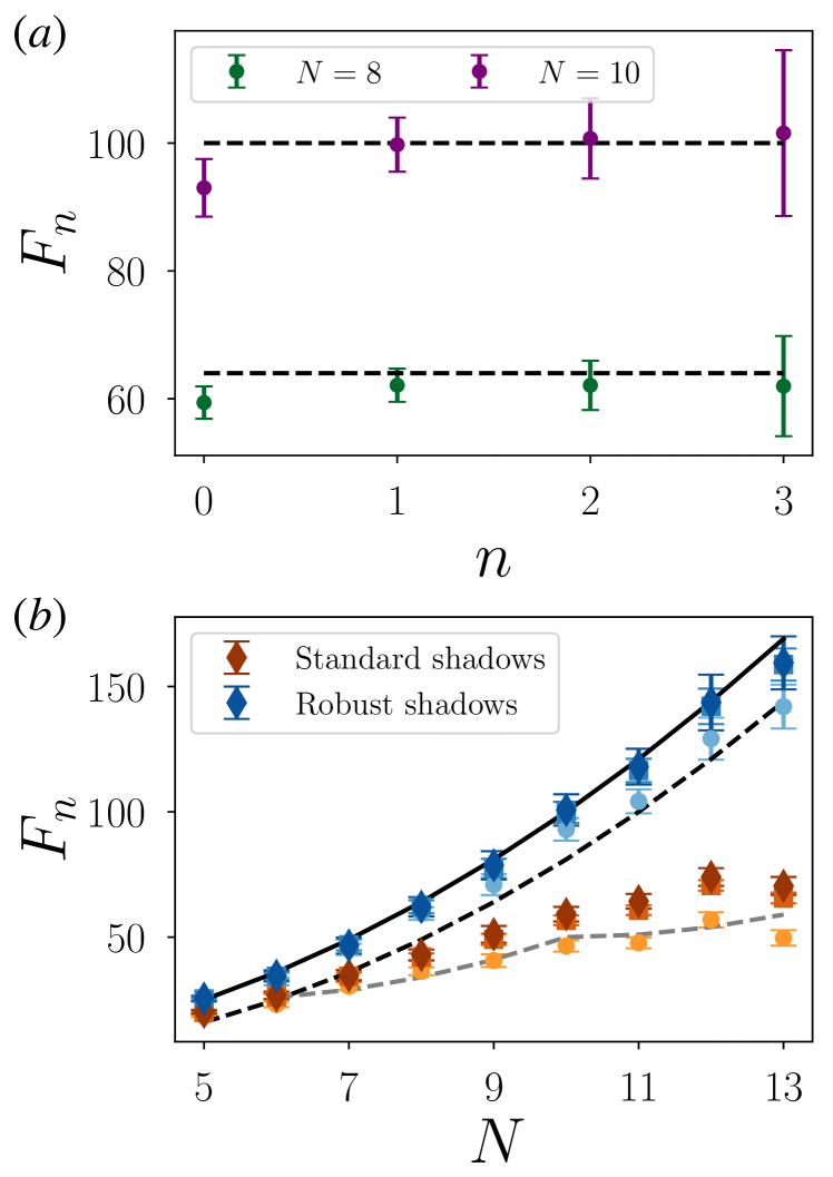
Figure 2: Experimental results for the lower bounds of the QFI for the GHZ state. $(a)$ Convergence of $F_{n}$ as a function of $n$ for $N=8,10$ qubits (green and violet respectively). $(b)$ $F_{2}$, $F_{1}$, $F_{0}$ (dark to light with diamond, square and circle respectively) as a function of the number of qubits $N$. The solid line is the exact value of the QFI $F_{Q}=N^{2}$ for pure GHZ states. The dashed black line corresponds to the entanglement witness $\Gamma(N,k=N-1)=(N-1)^{2}$ above which the state is considered to be GME. The dashed grey line corresponds to the entanglement witness $\Gamma(N,k=5)$ above which we detect a state to be at least 6-partite entangled. The details of the experimental protocol are described in Sec. I.

In this section we describe the experimental results that were performed on IBM superconducting processors. As mentioned before, we will consider two states: the GHZ state in Sec. III.1 and the ground state of the TFIM at the critical point in Sec. III.2.

III.1 GHZ states

The Greenberger-Horne-Zeilinger (GHZ) state has become a fundamental resource for various quantum information processing tasks, including quantum teleportation [62, 63], quantum error correction [64, 65], and quantum cryptography [66]. It can be written as

$$\ket{\text{GHZ}}=\frac{1}{\sqrt{2}}\left(\ket{0}^{\otimes N}+\ket{1}^{\otimes N}\right).$$ (9)

Remarkably, GHZ states are ideal candidates for quantum metrology as they saturate the value of the QFI $(F_{Q}=N^{2})$ and, thus, can be used to reach higher sensitivities in parameter estimation that scale as $\sim N^{-1}$ (known as Heisenberg limit), and is beyond the standard shot-noise limit $\sim N^{-1/2}$ [67, 2, 68].

By implementing randomized measurements, we experimentally estimate the QFI as a function of different system sizes $N$ and witness the presence of multipartite entanglement [2, 3, 5]. Until now, fidelity measurements have allowed to validate GME in GHZ states prepared on superconducting qubits [69, 70], 14 trapped ions [71], 18 photonic qubits [72] and other multipartite entangled states [73, 74, 75, 76]. Additionally, GME states can also be verified via multiple coherences for GHZ states [77, 78].

We show our experimental results in Fig. 2. In panel $(a)$ we represent $F_{n}$ ($n=0,1,2,3$) for the GHZ state prepared on a system of $N=8$ (green) and $N=10$ (violet) qubits respectively. The dashed black line corresponds to the exact theoretical value of the QFI ($F_{Q}=N^{2}$). We observe the convergence of $F_{n}$ to the value of the QFI at fixed $N$ within error bars. In all this work, the plotted statistical error bars correspond to one standard deviation of the mean. However, increasing the order $n$, the statistical error on the estimation increases, at fixed measurement budget. This is due to the fact that variance of the estimators in Eq. (8) increases with $n$. This is thoroughly discussed in Ref. [60]. In Fig. 2$(b)$ we show the experimental measurements of $F_{2},\,F_{1}$, and $F_{0}$ (dark to light) on the prepared GHZ state as a function of $N$. The black thick line provides the ideal scaling of the QFI ($F_{Q}=N^{2}$) for pure GHZ states. The black dashed line, instead, denotes the entanglement witness $\Gamma(N,k=N-1)$ that scales as $(N-1)^{2}$ above which we can consider our prepared states to be GME. The experimental points correspond to the measured bounds for two different cases: mitigated results through our calibration step in blue, raw data without performing the calibration step in orange. We observe that the mitigated data used to estimate $F_{n}$ violates the necessary entanglement witness to be GME for any size $N$, hence all our prepared states have an entanglement depth of $k=N$. Thus, we demonstrate the presence of multipartite entanglement through the estimation of converging lower bounds to the QFI, whose convergence to the true value has been shown in Fig. 2$(a)$.

Analysing the raw data (orange points in Fig. 2$(b)$) that are prone to errors during the randomized measurement protocol gives us lower estimations of the bounds. They do not violate the GME threshold and do not follow the expected scaling seen for the mitigated data points. This shows that the error mitigation in the measurement protocol is decisive and useful to estimate underlying properties of the prepared quantum states. In the case of the analysis of the raw data, we can assert from the witness bounds in Ref. [2, 3] that our prepared state contains an entanglement depth of $k=6$ for $N\geq 6$. Importantly, in App. E.3, we show the estimation of the lower bounds in the case when the calibration (step (i) in Fig. 1) is done entirely at the beginning and is followed by the experiment (step (ii) in Fig. 1). We observe clearly that performing the calibration in multiple iterations provides better results for larger system sizes where the full experimental duration starts to increase.

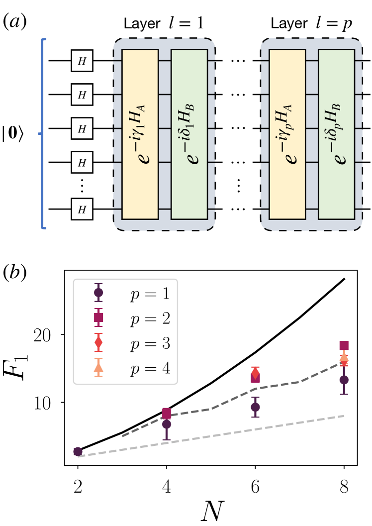
Figure 3: Experimental results for the lower bounds of the QFI for the ground state of the Ising model at the critical point. $(a)$ Sketch of the circuit used to variationally prepare the ground state. $(b)$ Results for $F_{1}$ estimated with the robust estimator as a function of the number of qubits $N$, for different circuit depth $p$. The lines correspond to (solid black) exact QFI value, (dashed dark grey) detects entanglement depth $k=3$ ($F_{Q}=\Gamma(N,2)$), (dashed grey) detects entanglement ($F_{Q}=N$). The measurement budget employed is described in Sec. I.

III.2 Ground state of the critical TFIM

To complement the estimation of the QFI to more generic quantum many-body states, we study here the behaviour of the QFI at a critical point that presents rich structure of multipartite entanglement [8, 7, 79, 80]. In particular, we consider the TFIM Hamiltonian

$$H=-J\sum_{j}\sigma^{z}_{j}\sigma^{z}_{j+1}-h\sum_{j}\sigma^{x}_{j},$$ (10)

where $h$ is the transverse field and we set $J=1$. It displays a quantum phase transition at $h=1$ that manifests as a growth of multipartite entanglement that can be witnessed by the QFI [6, 80]. We employ classical numerical simulations for estimating variationally the ground state at the critical point, optimizing the parameters of a circuit as it is done for the quantum adiabatic optimization algorithm [37] (See Fig. 3$(a)$). We study the interplay between the depth $p$ of the circuit realized and the approximation of the ground state. Indeed, in recent times there has been significant interest in measuring the QFI in states prepared through variational circuits on current quantum processors [81, 82, 83].

The preparation of the state entails a series of unitary quantum evolutions under the non-commuting terms in Eq. (10), i.e. $H_{A}=-J\sum_{j}\sigma^{z}_{j}\sigma^{z}_{j+1}$ and $H_{B}=-h\sum_{j}\sigma^{x}_{j}$, that are applied to an initial quantum state $\ket{\psi_{0}}$ (Fig. 3$(a)$). The final state after $p$ layers can be written as:

$$\ket{\psi(\bm{\delta},\bm{\gamma})}=\prod_{l=1}^{p}\mathrm{e}^{-i\delta_{l}H_{B}}\mathrm{e}^{-i\gamma_{l}H_{A}}\ket{\psi_{0}}$$ (11)

where the ‘angles’ $\delta_{l}$ and $\gamma_{l}$ are variational parameters used in the $l$-th layer to minimise the final energy $\bra{\psi(\bm{\delta},\bm{\gamma})}H\ket{\psi(\bm{\delta},\bm{\gamma})}$. The optimal parameters are found employing a suitable optimization algorithm. In the particular case of our target state, it has been shown that it could be prepared exactly in $p=N/2$ steps, where $N$ is the total number of qubits [84].

In Fig. 3$(b)$ we plot $F_{1}$ for different values of the depth $p$ of the circuits as a function of the number of qubits $N$ for the robust estimator. The solid black line represents the numerical exact value of the QFI. Our first observation consists in remarking that we generate and certify the presence of entanglement in all our prepared states as $F_{Q}\geq F_{1}\geq N$ [11] within error bars for all values of depths $p$ and system size $N$. The corresponding threshold is shown as a dashed grey line in the plot.

For all system-sizes, states prepared with a circuit depth of $p=2$ have the highest measured value of $F_{1}$ compared to other circuit depths. A further increase in the circuit depth $p$, incorporates more noisy gates that reduce the fidelity of the prepared state compared to its true target state. This results in a decrease of the QFI estimation compromised by the noisy state preparation that is captured very well in Fig. 3$(b)$. We explicitly see for $p=3,\,4$ a compatible estimation of $F_{1}$ within error bars compared to the former case of $p=2$ that shows a signature of noise and decoherence in the preparation of the state. In fact, in the ideal scenario, increasing the number of layers should guarantee better convergence to the target state.

Importantly, we establish the presence of multipartite entanglement via $F_{1}$ as we violate the entanglement witness $F_{1}>\Gamma(N,k=2)$. This confirms the presence of an entanglement depth of $k=3$ for all prepared states of system-size $N>2$, as the experimental points are above the witness depicted by the dashed dark grey line in Fig. 3$(b)$. Thus our method allows to quantify the true metrological power in form of generating multipartite entanglement in our noisy prepared states. Additionally, the qualitative behaviour of the other estimators ($F_{0}$ and $F_{2}$) is the same and, we provide the experimental results in App. E.2, together with the measurement of the purity of the prepared state.

IV Conclusions

In this paper, we have demonstrated the first experimental estimation of the quantum Fisher information (QFI). This was achieved on a quantum processor with up to 13 qubits based on the measurements of a converging series of polynomial lower bounds. By combining advanced methods from the randomized measurement toolbox, we have been able to overcome drifting gate and readout errors, and obtain a robust and unbiased estimator for the QFI.

We applied our method to two different states: GHZ states and the ground state of the TFIM at the critical point. For the former, our measurements are in perfect agreement with theoretical predictions and allow us to witness the presence of multipartite entanglement, so far achieved only by fidelity measurements. With the error mitigation procedure that we introduce here, we observed that all our prepared GHZ states were GME. In the variational preparation of the ground state of the critical TFIM , we utilize the estimated QFI to observe an interesting trade-off. While the theoretical approximation accuracy of the ground state increases with the circuit depth and is optimal at depth $p=N/2$, the best estimation of the theoretically predicted ground state QFI is obtained with a smaller circuit depth. We attribute this effect to noise and decoherence increasing with circuit depth as well.

We stress that our method is well-suited for following the drifting errors in the hardware as experimentally shown in App. C.1. Performing a calibration at the beginning of the whole experiment is not sufficient for taming and understanding the errors in the randomized measurement protocol, of which we show evidence in App. E.3.

Furthermore, our approach is not limited to the measurement of the QFI. Our results extend easily to obtain robust and unbiased estimators for arbitrary non-linear multi-copy functionals that can be expressed as observables acting on multiple copies of the quantum state. This extends the applicability of our methodology beyond the QFI and opens up possibilities for other quantum information processing tasks such as exploring many-body entanglement phases by measuring partial transpose moments [50]. Additionally, as the robust calibration method is memory efficient, it can be performed to measure observables such as energy estimation of the ground state of quantum chemistry Hamiltonians prepared on large-scale quantum devices [85, 86] that can be further boosted by employing common randomized measurements techniques [59]. Finally, our method could be used in combination with machine-learning approaches to learn complex phases of matter with robust shadows [87, 88].

Appendix A Converging series of lower bounds of the QFI

As shown in Ref. [34], the QFI can be expanded in terms of a Taylor series in the eigenvalues $\lambda_{\mu}$ of the density matrix $\rho=\sum_{\mu}\lambda_{\mu}\outerproduct{\mu}{\mu}$. This reads as:

$$F_{Q}=2\sum_{\ell=0}^{\infty}\sum_{(\mu,\nu),\lambda_{\mu}+\lambda_{\nu}>0}(\lambda_{\mu}-\lambda_{\nu})^{2}(1-\lambda_{\mu}-\lambda_{\nu})^{\ell}|\bra{\mu}A\ket{\nu}|^{2}.$$ (12)

We note that each term in the infinite sum is positive. Truncating the summation at a finite value $n$, we thus obtain a converging series of polynomial lower bounds $F_{n}$ that can be measured experimentally:

$$F_{n}=2\sum_{\ell=0}^{n}\sum_{(\mu,\nu),\lambda_{\mu}+\lambda_{\nu}>0}(\lambda_{\mu}-\lambda_{\nu})^{2}(1-\lambda_{\mu}-\lambda_{\nu})^{\ell}|\bra{\mu}A\ket{\nu}|^{2}=2\sum_{q=0}^{n}\binom{n+1}{q+1}(-1)^{q}\sum_{m=0}^{q+2}C_{m}^{(q)}\Tr(\rho^{q+2-m}A\rho^{m}A),$$ (13)

where we have introduced the coefficients $C_{m}^{(q)}=\binom{q}{m}-2\binom{q}{m-1}+\binom{q}{m-2}$, with the binomial coefficients defined such that $\binom{q}{m^{\prime}}=0$ if $m^{\prime}<0$ or $m^{\prime}>q$. The last equality can be proven by injecting the eigenvalue decomposition of $\rho$ in the right-hand side and rearranging the sums [34].

Appendix B Derivation of the robust shadow estimator with local noise

In this section we construct the robust classical shadow estimator given in Eq. (3), equivalent to the one presented for the first time in Ref. [38]. We consider a situation where we have performed randomized measurements on a $N$-qubit state $\rho$, which are affected by noise. We assume that the noise is gate-independent, Markovian and stationary within each iteration, and that it occurs between the random unitaries and the measurements (not before the unitaries). This ensures that we can model noisy randomized measurements as $\mathcal{M}\circ\Lambda^{(i)}\circ\mathcal{U}^{(r)}$ where $\mathcal{U}^{(r)}$ is the ideal unitary channel describing the application of ideal random unitaries $U^{(r)}$, $\Lambda^{(i)}$ is the noise channel in iteration $i$, encapturing gate noise and readout errors, and $\mathcal{M}$ is the measurement channel, describing an ideal computational basis measurement [38]. In addition, we assume local noise, i.e. the noise channel decomposes as $\Lambda^{(i)}=\Lambda^{(i)}_{1}\otimes\dots\otimes\Lambda^{(i)}_{N}$ and local random unitaries, i.e. the ideal unitary channel is realized with local unitary transformations $U^{(r)}=U^{(r)}_{1}\otimes\dots\otimes U^{(r)}_{N}$. Here, the local unitaries $U_{j}^{(r)}$ are sampled independently and uniformly from the circular unitary ensemble, i.e. the Haar measure on the unitary group $U(2)$.

As described in the main text, we employ first a calibration protocol, equivalent to the one described in Ref. [38], to characterize the local noise channel $\Lambda^{(i)}$ in terms of $N$ parameters $G^{(i)}_{j}$. To perform this calibration, we assume that the state $\ket{\mathbf{0}}=\ket{0}^{\otimes N}$ can be prepared with a high fidelity in our experiment. The calibration results are then used to build an unbiased estimator $\hat{\rho}$ of the density matrix $\rho$ – a robust classical shadow – from randomized measurements performed on $\rho$, that mitigates the noise errors induced by $\Lambda^{(i)}$.

In the remainder of this section, we drop the superscript $i$ denoting the iteration of the experiment to simplify the notation.

B.1 Robust shadow from randomized measurements

Under the noise assumptions described above, noisy randomized measurements provide access to the probability distribution of the measured bit-strings $\mathbf{s}=(s_{1},\dots,s_{N})$, conditioned on the application of a local random unitary $U^{(r)}=U_{1}^{(r)}\otimes\dots\otimes U_{N}^{(r)}$:

$$P_{\Lambda}(\mathbf{s}|U^{(r)})=\bra{\mathbf{s}}\Lambda(U^{(r)}\rho\,{U^{(r)}}^{\dagger})\ket{\mathbf{s}}=\Tr(\rho\,{U^{(r)}}^{\dagger}\Lambda^{*}(\outerproduct{\mathbf{s}}{\mathbf{s}})U^{(r)}),$$ (14)

where $\Lambda$ is the trace-preserving noise channel and $\Lambda^{*}$ is its adjoint. We aim to construct an unbiased estimator of $\rho$ – robust classical shadow – in terms of the statistics of $P_{\Lambda}(\mathbf{s}|U^{(r)})$. We choose an ansatz of the form

$$\tilde{\rho}^{(r)} =\sum_{\mathbf{s}}P_{\Lambda}(\mathbf{s}|U^{(r)})\,{U^{(r)}}^{{\dagger}}O(\mathbf{s})U^{(r)}$$ (15)

$$=\sum_{\mathbf{s}}\Tr(\rho\,{U^{(r)}}^{\dagger}\Lambda^{*}(\outerproduct{\mathbf{s}}{\mathbf{s}})U^{(r)})\,{U^{(r)}}^{{\dagger}}O(\mathbf{s})U^{(r)}$$

$$=\sum_{\mathbf{s}}\Tr_{1}\left(\left(\rho\otimes\mathbb{1}\right)({U^{(r)}}^{{\dagger}})^{\otimes 2}\big{[}\Lambda^{*}(\outerproduct{\mathbf{s}}{\mathbf{s}})\otimes O(\mathbf{s})\big{]}{U^{(r)}}^{\otimes 2}\right)$$

with $O(\mathbf{s})=\bigotimes_{j}O_{j}(s_{j})$ being a local hermitian operator, which we take to be diagonal in the computational basis, and $\Tr_{1}$ denoting the partial trace over the first copy of the $N$-qubit system. The ensemble average over the random unitaries $U^{(r)}$ yields

$$\mathbb{E}[\tilde{\rho}^{(r)}]=\Tr_{1}\left[(\rho\otimes\mathbb{1})\Phi^{(2)}\left(\sum_{\mathbf{s}}\Lambda^{*}(\outerproduct{\mathbf{s}}{\mathbf{s}})\otimes O(\mathbf{s})\right)\right]=\Tr_{1}\left[(\rho\otimes\mathbb{1})\Phi^{(2)}(Q)\right]$$ (16)

with

$$Q=\sum_{\mathbf{s}}\Lambda^{*}(\outerproduct{\mathbf{s}}{\mathbf{s}})\otimes O(\mathbf{s})=\bigotimes_{j=1}^{N}\left[\sum_{s_{j}=0,1}\Lambda_{j}^{*}(\outerproduct{s_{j}}{s_{j}})\otimes O_{j}(s_{j})\right]=\bigotimes_{j=1}^{N}Q_{j}.$$ (17)

Here, we used the local noise assumption (noting that $\Lambda^{*}=(\bigotimes_{j}\Lambda_{j})^{*}=\bigotimes_{j}\Lambda_{j}^{*}$) and $\Phi^{(2)}(\cdot)=\mathbb{E}[({U^{(r)}}^{{\dagger}})^{\otimes 2}(\cdot){U^{(r)}}^{\otimes 2}]$ denotes the two-copy local unitary ‘twirling channel’ [90]. It evaluates to

$$\Phi^{(2)}(Q)=\left(\frac{1}{3}\right)^{N}\bigotimes_{j=1}^{N}\left(\left(\mathrm{Tr}(Q_{j})-\frac{1}{2}\mathrm{Tr}(\mathbb{S}_{j}Q_{j})\right)\mathbb{1}^{(2)}_{j}+\left(\mathrm{Tr}(\mathbb{S}_{j}Q_{j})-\frac{1}{2}\mathrm{Tr}(Q_{j})\right)\mathbb{S}_{j}\right)$$ (18)

with the swap operator $\mathbb{S}_{j}=\sum_{s_{j_{1}},s_{j_{2}}}\outerproduct{s_{j_{2}}}{s_{j_{1}}}\otimes\outerproduct{s_{j_{1}}}{s_{j_{2}}}$ acting on two copies of qubit $j$ and $\mathbb{1}^{(2)}_{j}=\mathbb{1}_{j}\otimes\mathbb{1}_{j}$ the identity.

The estimator $\tilde{\rho}^{(r)}$ is an unbiased estimator of $\rho$ if the average over the Haar random unitaries yields the true density matrix of the quantum state, $\mathbb{E}\left[\tilde{\rho}^{(r)}\right]=\rho$. Observing that $\Tr_{1}\left(\left(\rho\otimes\mathbb{1}\right)\mathbb{S}\right)=\rho$ where $\mathbb{S}=\bigotimes_{j=1}^{N}\mathbb{S}_{j}$ is the swap operator between two copies of the entire system, we thus find, from Eq. (16), that the estimator is unbiased for any state $\rho$ if and only if $\Phi^{(2)}(Q)=\mathbb{S}$, or equivalently, using Eq. (18),

$$\left(\mathrm{Tr}(Q_{j})-\frac{1}{2}\mathrm{Tr}(\mathbb{S}_{j}Q_{j})\right)\mathbb{1}^{(2)}_{j}+\left(\mathrm{Tr}(\mathbb{S}_{j}Q_{j})-\frac{1}{2}\mathrm{Tr}(Q_{j})\right)\mathbb{S}_{j}=3\mathbb{S}_{j}\quad\forall j.$$ (19)

On top of the assumption that $O_{j}(s_{j})$ is diagonal in the computational basis, we further assume that it is of the form $O_{j}(s_{j})=\alpha_{j}\outerproduct{s_{j}}{s_{j}}+\beta_{j}\mathbb{1}$, with $\alpha_{j}$, $\beta_{j}$ real numbers that do not depend on $s_{j}$. With this, we can evaluate the terms appearing in Eq. (19) above as follows:

$$\Tr(Q_{j}) =\sum_{s_{j}}\Tr(\Lambda^{*}(\outerproduct{s_{j}}{s_{j}}))\Tr(O_{j}(s_{j}))=\sum_{s_{j}}\Tr(\Lambda^{*}(\outerproduct{s_{j}}{s_{j}}))(\alpha_{j}+2\beta_{j})$$

$$=\Tr(\Lambda(\mathbb{1}))(\alpha_{j}+2\beta_{j})=2\alpha_{j}+4\beta_{j},$$ (20)

$$\Tr(\mathbb{S}_{j}Q_{j}) =\sum_{s_{j}}\Tr(\Lambda^{*}(\outerproduct{s_{j}}{s_{j}})O_{j}(s_{j}))$$

$$=\alpha_{j}\sum_{j}\Tr(\Lambda^{*}(\outerproduct{s_{j}}{s_{j}})\outerproduct{s_{j}}{s_{j}})+2\beta_{j}=2\alpha_{j}G_{j}+2\beta_{j},$$ (21)

where we have used also that the noise channel is trace preserving and $\Tr(\mathbb{S}A\otimes B)=\Tr(AB)$. Here, we have introduced the quantity

$$G_{j}=\frac{1}{2}\sum_{s_{j}}\bra{s_{j}}\Lambda_{j}(\outerproduct{s_{j}}{s_{j}})\ket{s_{j}},$$ (22)

that contains all the relevant information on the noise acting on qubit $j$ during the randomized measurement protocol, and which we interpret as the average ‘survival probability’ of the two basis states of qubit $j$. Thus, to characterise the noise that affects the experimental protocol we only need to learn how it acts on the computational basis states $\ket{s_{j}}$. With the above expressions, inverting Eq. (19) gives

$$\alpha_{j}=\frac{3}{2G_{j}-1},\qquad\beta_{j}=\frac{G_{j}-2}{2G_{j}-1}.$$ (23)

Inserting this into Eq. (15), we finally can write the estimator $\tilde{\rho}$ as

$$\tilde{\rho}^{(r)} =\sum_{\mathbf{s}}P_{\Lambda}(\mathbf{s}|U^{(r)})\bigotimes_{j=1}^{N}\left(\alpha_{j}{U^{(r)}_{j}}^{{\dagger}}\outerproduct{s_{j}}{s_{j}}U^{(r)}_{j}+\beta_{j}\mathbb{1}\right)$$ (24)

$$=\sum_{\mathbf{s}}P_{\Lambda}(\mathbf{s}|U^{(r)})\bigotimes_{j=1}^{N}\left(\frac{3}{2G_{j}-1}{U^{(r)}_{j}}^{{\dagger}}\outerproduct{s_{j}}{s_{j}}U^{(r)}_{j}+\frac{G_{j}-2}{2G_{j}-1}\mathbb{1}\right).$$

In the absence of noise $G_{j}=1$, $\forall j$, so that the usual formula for the estimator of the density matrix from randomized measurements is recovered: $O_{j}(s_{j})=3\outerproduct{s_{j}}{s_{j}}-\mathbb{1}$ [56, 58]. For a fully depolarising channel, on the other hand, one gets $G_{j}=1/2$, in which case we are not able to extract any information by measuring the state as the coefficients in Eq. (23) diverge.

B.2 Calibration step

The parameters in Eq. (23) rely on the estimation of $G_{j}$. It is based on the calibration procedure described in the main text (Sec. I). In a nutshell, the system is prepared in a state with high fidelity, namely $\ket{\mathbf{0}}\equiv\ket{0}^{\otimes N}$, and the randomized measurement protocol is applied. We show here that $G_{j}$ can be directly linked to the random unitaries $U^{(r)}=U_{1}^{(r)}\otimes\dots\otimes U_{N}^{(r)}$, with $r=1,\dots,N_{U}$, and the bit-strings of measurement outcomes $\mathbf{s}^{(r,m)}=(s^{(r,m)}_{1},\dots,s^{(r,m)}_{N})$ with $m=1,\dots,N_{M}$.

Let us introduce the following quantity

$$C_{j}=\sum_{s_{j}=0,1}\mathbb{E}\left[\bra{s_{j}}\Lambda_{j}(U^{(r)}_{j}\outerproduct{0}{0}{U^{(r)}_{j}}^{{\dagger}})\outerproduct{s_{j}}{s_{j}}U^{(r)}_{j}\outerproduct{0}{0}{U^{(r)}_{j}}^{{\dagger}}\ket{s_{j}}\right],$$ (25)

where $\ket{0}$ represents the calibration state of the single qubit $j$ and $\mathbb{E}[\cdot]$ is the average over the circular unitary ensemble. We can define an estimator as:

$$\hat{C}_{j}=\frac{1}{N_{U}}\sum_{r}\sum_{s_{j}=0,1}\hat{P}(s_{j}|U_{j}^{(r)})P(s_{j}|U_{j}^{(r)}),$$ (26)

where $\hat{P}(s_{j}|U_{j}^{(r)})=\sum_{m=1}^{N_{M}}\frac{\delta_{s_{j},s_{j}^{(r,m)}}}{N_{M}}$ is the estimated (noisy) Born probability and $P(s_{j}|U_{j}^{(r_{i})})=|\bra{s_{j}}U^{(r)}_{j}\ket{0}|^{2}$ is the theoretical (noiseless) one. The information on the noise is contained in $\hat{P}(s_{j}|U_{j}^{(r)})$, that approaches the theoretical noisy Born probability $P_{\Lambda}(s_{j}|U_{j}^{(r)})$ in the limit $N_{M}\rightarrow\infty$. Thus, since with our noise model $\mathbb{E}_{\rm QM}[\hat{P}(s_{j}|U^{(r)})]=\bra{s_{j}}\Lambda_{j}(U^{(r)}_{j}\outerproduct{0}{0}{U^{(r)}_{j}}^{{\dagger}})\ket{s_{j}}$, we have $\mathbb{E}\big{[}\mathbb{E}_{\rm QM}[\hat{C}_{j}]\big{]}=C_{j}$, i.e $\hat{C_{j}}$ is an unbiased estimator for $C_{j}$. Here $\mathbb{E}_{\rm QM}[\cdot]$ is the quantum mechanical average over the Born probabilities. We note that under the (idealized) assumption of strictly gate-independent noise (same noise channel $\Lambda_{j}$ for any $U^{(r)}_{j}$, including the idle gate $\mathbb{1}_{j}$), we could measure $G_{j}$ directly from its definition, Eq. (22). In practice, we expect that $C_{j}$ (and its estimator $\hat{C}_{j}$) captures the actual noise acting during the measurement stage more faithfully, as exactly the same experimental resources are employed and any weakly gate dependent noise is averaged (twirled) to yield approximately the same gate-independent average noise channel, $\mathbb{E}[\Lambda_{U}(\rho)]\approx\Lambda(\mathbb{E}[U\rho U^{\dagger}])$. We refer to more details on gate-dependent noise in Ref. [38].

Let us now link $C_{j}$ and the quantity $G_{j}$ in Eq. (22). We observe that $C_{j}$ can be written as

$$C_{j}=\mathbb{E}\left[\bra{0}^{\otimes 2}{{U^{(r)}_{j}}^{{\dagger}}}^{\otimes 2}\left(\sum_{s_{j}=0,1}\Lambda_{j}^{*}\left(\outerproduct{s_{j}}{s_{j}}\right)\otimes\outerproduct{s_{j}}{s_{j}}\right){U^{(r)}_{j}}^{\otimes 2}\ket{0}^{\otimes 2}\right],$$ (27)

where we have used the property $\mathrm{Tr}(\Lambda(A)B)=\mathrm{Tr}(A\Lambda^{*}(B))$. As in the previous section, we can express the average in $C_{j}$ over unitaries in terms of a twirling channel $\Phi_{j}^{(2)}(Q_{j})$ (a single-qubit version of the 2-copy channel $\Phi$ introduced before). In this case we write the two-copy operator $Q=\bigotimes_{j=1}^{N}Q_{j}$ with $Q_{j}=\sum_{s_{j}=0,1}\Lambda_{j}^{*}\left(\outerproduct{s_{j}}{s_{j}}\right)\otimes\outerproduct{s_{j}}{s_{j}}$. Using again the twirling formula in Eq. (18) (now for two copies of a single qubit) one obtains

$$C_{j}=\bra{0}^{\otimes 2}\Phi_{j}^{(2)}\left(\sum_{s_{j}}\Lambda^{*}(\outerproduct{s_{j}}{s_{j}})\otimes\outerproduct{s_{j}}{s_{j}}\right)\ket{0}^{\otimes 2}=\frac{1+G_{j}}{3}.$$ (28)

The link between $C_{j}$ and $G_{j}$ being clear, one can define an estimator for $G_{j}$ in terms of the one for $C_{j}$ in Eq. (26):

$$\hat{G}_{j}=3\;\hat{C}_{j}-1.$$ (29)

In the absence of noise one can check that $G_{j}=1$ and $C_{j}=\frac{2}{3}$, $\forall j=1,\dots,N$ [58]. We remark here that all our results are compatible with the ones in Ref. [38], where a slightly different formalism has been employed.

B.3 Enhanced estimation of $G_{j}$

We show here that the statistical accuracy of the estimator of $G_{j}$ can be improved by making use of common randomized numbers [59] to define an estimator with smaller variance with respect to the one introduced in Ref. [38] and considered above – namely, $\hat{G}_{j}$.

Suppose one aims to estimate the expectation value $\mathbb{E}[X]$ of a random variable $X$. If we estimate $\mathbb{E}[X]$ by averaging over multiple samples $X_{i}$, the statistical error is quantified by the variance $\mathrm{Var}[X]$. Now, assume we have access to a random variable $Y$, strongly correlated with $X$ whose average value $\mathbb{E}[Y]$ is known. We can estimate $\mathbb{E}[X]$ with reduced variance $\mathrm{Var}[X-Y]<\mathrm{Var}[X]$ by averaging the random variable $X-Y+\mathbb{E}[Y]$ over commonly sampled variables ${X_{i},Y_{i}}$. We employ this trick for $G_{j}$, to define an enhanced estimator with reduced variance compared to $\hat{G}_{j}$ (and the one presented in Ref. [38]) if the noise is weak.

Let us introduce for that the quantity

$$B_{j}=\frac{1}{N_{U}}\sum_{r}\sum_{s_{j}=0,1}P(s_{j}|U_{j}^{(r)})^{2}$$ (30)

with $P(s_{j}|U_{j}^{(r)})=|\bra{s_{j}}U^{(r)}_{j}\ket{0}|^{2}$ as above, which is equivalent to $C_{j}$ (Eq. (26)) in absence of noise and in the limit of infinite measurements $N_{M}\rightarrow\infty$. With this, we then define

$$\hat{\mathcal{C}}_{j}=\hat{C}_{j}-B_{j}+\mathbb{E}[B_{j}].$$ (31)

Here $\hat{\mathcal{C}}_{j}$ and $\hat{C}_{j}$ have the same expectation value, namely $\mathbb{E}[\hat{\mathcal{C}}_{j}]=\mathbb{E}[\hat{C}_{j}]=C_{j}$, but the variance of $\hat{\mathcal{C}}_{j}$ is smaller because $\hat{C}_{j}$ and $B_{j}$ are positively correlated. We can thus construct the new estimator

$$\hat{\mathcal{G}}_{j}=3\;\hat{\mathcal{C}}_{j}-1,$$ (32)

which can be seen to be equivalent to Eq. (5) in the main text, given that $\mathbb{E}[B_{j}]=\bra{0}^{\otimes 2}\Phi_{j}^{(2)}\left(\sum_{s_{j}}\outerproduct{s_{j}}{s_{j}}\otimes\outerproduct{s_{j}}{s_{j}}\right)\ket{0}^{\otimes 2}=\frac{2}{3}$ (as in Eq. (28), in the absence of noise). The variance of estimators obtained from such common randomized measurements has been studied analytically in Ref. [59], where it was shown that involving positively correlated random variables, as above, indeed allows one to significantly reduce the variance upper bounds. In the following section we compare based on our experimental data this estimator with the one introduced in Eq. (29).

B.4 Experimental comparison of the estimators $\hat{G}_{j}$ and $\hat{\mathcal{G}}_{j}$

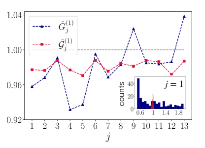
Figure 4: Comparison of $G_{j}$ using the enhanced estimator $\hat{\mathcal{G}}_{j}$ and the previous estimator $\hat{G}_{j}$ for a 13-qubit state on ‘ibm_prague’. The quantities are measured according to the calibration protocol described in Sec. I and depicted in Fig. 1. $N_{U}^{\mathrm{tot}}=N_{I}N_{U}=27000$ (number of unitaries in the randomized measurement protocol) and $N_{M}=1000$ (number of measurements per unitary). In the inset we compare the estimators for iteration $i=1$, i.e. $\hat{G}^{(1)}_{j}$ (blue) and $\hat{\mathcal{G}}^{(1)}_{j}$ (red), for the first qubit ($j=1$) by plotting a histogram where each occurrence corresponds to an element of the sum over $r$ in Eq. (26) for $\hat{G}^{(1)}_{j}$, and of the analogous sum for $\hat{\mathcal{G}}^{(1)}_{j}$.

Let us consider the $N=13$ qubit experiment that has been performed on the ‘ibm_prague’ processor. We have performed a calibration of the device as described in Sec. I and depicted in the step (i) of Fig. 1. For each iteration $i=1,\dots,N_{I}$ and for each applied unitary $U^{(r_{i})}$ ($r_{i}=1,\dots,N_{U}$), we collect $N_{M}=1000$ bit-strings of measurement outcomes. From the unitaries and the bit-strings we compute the quantities $\hat{G}^{(i)}_{j}$ and $\hat{\mathcal{G}}^{(i)}_{j}$ as defined above, which contain the information about the local errors in the measurement protocol within each iteration $i$.

In Fig. 4 we show the comparison of the two estimators, for iteration $i=1$ and all the qubits ($j=1,\dots,13$). In the inset we show a comparison of the histograms of he values that build up $\hat{G}^{(1)}_{j}$ and $\hat{\mathcal{G}}^{(1)}_{j}$ for the first qubit ($j=1$), where each point corresponds to an element of the sum over $r$ in Eq. (26) for $\hat{G}^{(1)}_{j}$, and of the analogous sum for $\hat{\mathcal{G}}^{(1)}_{j}$. Remarkably, we observe that the contributions to $\hat{\mathcal{G}}_{1}^{(1)}$ are much less spread than those of $\hat{G}^{(1)}_{1}$; in particular the contributions to $\hat{G}^{(1)}_{1}$ range in $\sim(0.6,1.8)$, while the $\hat{\mathcal{G}}_{1}^{(1)}$ counts are sharply peaked around $\sim 1$. We argue this is due to the trick of common random numbers [59] employed to define $\hat{\mathcal{G}}_{j}^{(i)}$, which in general allows to reduce the variance of the estimator. The same holds for any qubit $j$.

Appendix C Experimental results on the noise

In this section we perform an experimental analysis on the noise in the quantum platform we employ. We investigate the time dependence of the noise, noticing huge fluctuations in the quantities we use to estimate the errors, and we observe that the most important contribution to the single qubit error can be identified to be caused due to readout errors.

C.1 Verification of the time dependence of the noise in ‘ibm_prague’

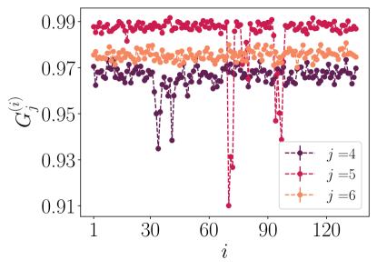
Figure 5: $G_{j}^{(i)}$ as a function of the iteration $i$ for a 13-qubit state on ‘ibm_prague’. The quantity is estimated from the calibration data of the protocol depicted in Fig. 1, using the estimator $\hat{\mathcal{G}}^{(i)}_{j}$ of Eq. (5). Here $N_{U}^{\mathrm{tot}}=N_{I}N_{U}=27000$ (number of unitaries in the randomized measurement protocol) and $N_{M}=1000$ (number of measurements per unitary). We present the result for qubits $j=4,5,6$.

Let us consider again the $N=13$ qubit experiment that has been performed on the ‘ibm_prague’ processor. In Fig. 5 we study the behaviour of $G_{j}^{(i)}$ (estimated through $\hat{\mathcal{G}}_{j}^{(i)}$ of Eq. (5)) as a function of the iterations $i$. The error in the quantum device fluctuates in time, we want to verify that it is important to perform consecutive iterations of experiments to account for the temporal variations in gate and readout errors instead of performing a single calibration in advance. We plot $G_{j}^{(i)}$ as a function of $i$ for three different qubits, labeled by $j$. For $j=4,5$, we observe fluctuating events given $G_{j}^{(i)}$ as a function of the iterations $i$, hinting that it is important to follow the temporal fluctuations of the noise to provide reliable and robust estimations. This is not the case for all the qubits; e.g., we do not see such fluctuations for $j=6$ in the plot. Similar effects have been observed in other type of error mitigation protocols with superconducting qubits [91, 92].

C.2 Check on the origin of the noise

Our aim here is to study what is the most important source of errors in the randomized measurement protocol.

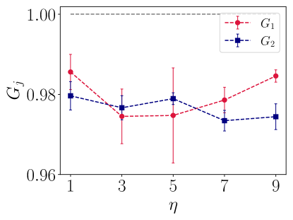
Figure 6: $G_{j}$ for a two-qubit system realized on ‘ibm_lagos’, as a function of the number of layers of unitaries $\eta$ applied to the initial state. We use the estimator $\hat{\mathcal{G}}_{j}$ of Eq. (5). A value compatible with 1 means that the noise can be neglected. Here $N_{U}=800$ (number of unitaries in the randomized measurement protocol) and $N_{M}=1000$ (number of measurements per unitary).

In Fig. 6 we consider a two-qubit system realised on the ‘ibm_lagos’ processor. We employ the calibration method described in Sec. I and depicted in Fig. 1. In order to discriminate between the various sources of noises, instead of applying a single unitary $U=\bigotimes_{j=1}^{N}U_{j}$, we employ several layers of unitaries, given by the number $\eta$ that are sampled independently and uniformly from the circular unitary ensemble. We measure the quantity $G_{j}$ as a function of the parameter $\eta$  using the enhanced estimator $\hat{\mathcal{G}}_{j}$ of Eq. (5). The rationale behind this approach is the following. We can write the noise channel $\Lambda$ acting during the measurement protocol as two separate contributions: one due to errors on the unitaries $\Lambda_{U}$ and one due to the readout $\Lambda_{\textrm{meas}}$ with $\Lambda=\Lambda_{\textrm{meas}}\circ\Lambda_{U}$. By applying $\eta$ layers of unitaries one would get $\Lambda(\eta)=\Lambda_{\textrm{meas}}\circ(\Lambda_{U})^{\eta}$. Following the effect of the noise as a function of $\eta$, we may be able to discriminate the contributions of $\Lambda_{U}$ and $\Lambda_{\textrm{meas}}$. This idea can be formalized based on a simple noise model defined by

$$\Lambda_{U}(\rho_{j})=(1-p_{U})\rho_{j}+\frac{p_{U}}{3}\sum_{\alpha}\sigma_{j}^{\alpha}\rho_{j}\sigma_{j}^{\alpha},$$ (33)

$$\Lambda_{\textrm{meas}}(\rho_{j})=(1-p_{\textrm{meas}})\rho_{j}+p_{\textrm{meas}}\sigma_{j}^{x}\rho_{j}\sigma_{j}^{x}.$$

Here $\sigma^{\alpha}=\sigma^{x},\sigma^{y},\sigma^{z}$ are single qubit Pauli matrices with $\rho_{j}$ being a single qubit density matrix. The action of the unitary gates is modeled as a depolarizing noise channel $\Lambda_{U}$ with parameter $p_{U}$, while the readout errors are described by bit flips that happen with probability $p_{\textrm{meas}}$. The full channel $\Lambda(\eta)(\rho_{j})$ applied on a single qubit state $\rho_{j}$ gives

$$\Lambda(\eta)(\rho_{j})=(1-\eta p_{U}-p_{\textrm{meas}})\rho_{j}+\frac{p_{U}\eta}{3}\sum_{\alpha}\sigma_{j}^{\alpha}\rho_{j}\sigma_{j}^{\alpha}+p_{\textrm{meas}}\sigma_{j}^{x}\rho_{j}\sigma_{j}^{x}.$$ (34)

We can compute explicitly the behavior of $G_{j}$ at first order in $p_{U},p_{\textrm{meas}}\ll 1$ and obtain

$$G_{j}(\eta)=1-\frac{2p_{U}}{3}\eta-p_{\textrm{meas}}.$$ (35)

We observe that the unitary contribution would monotonically decrease $G_{j}$ as a function of $\eta$ while the readout error yields a fixed shift by $p_{\textrm{meas}}$. From Fig. 6, we observe that $G_{j}$ remains essentially constant within error bars for different values of $\eta$, hence increasing the number of unitaries does not induce more noise (in terms of the parameter $G_{j}$) in the system. This suggests that the most relevant contribution to the noise in the randomized measurement protocol is due to readout errors.

Appendix D Verification of the validity of the assumption of local noise

In this section we propose a method to test the assumption of a local noise channel, i.e. $\Lambda=\bigotimes_{j=1}^{N}\Lambda_{j}$, that is based on analysing the statistical correlations among qubit pairs. We employ the calibration data that has been used for the mitigation of the QFI results on the prepared GHZ states. The section is structure as follows: At first we drop the assumption of locality, i.e. we consider a general noise channel $\Lambda$, and introduce a quantity $\tilde{R}$ that can be used for testing its locality; then, we provide an illustrative analytical example in the case of cross-talk errors for two qubits; finally, we show an experimental indication of the validity of the assumption of locality.

D.1 Derivation of the estimator of locality of noise

Let us start by extending Eq. (25) to measurements that act on the whole device, writing

$$\tilde{C}_{j} =\mathbb{E}\left[\sum_{s_{j}}\Tr[\bra{s_{j}}\Lambda(U^{(r)}\outerproduct{\mathbf{0}}{{\mathbf{0}}}{U^{(r)}}^{\dagger})\ket{s_{j}}]P(s_{j}|U_{j}^{(r)})\right]$$ (36)

$$=\mathbb{E}\left[\sum_{s_{j}}\Tr[\outerproduct{s_{j}}{s_{j}}\Tr_{k\neq j}(\Lambda(U^{(r)}\outerproduct{\mathbf{0}}{\mathbf{0}}{U^{(r)}}^{\dagger}))]P(s_{j}|U_{j}^{(r)})\right],$$

where $\mathbb{E}$ denotes the average over all local unitaries $U_{k}^{(r)}$’s and again $P(s_{j}|U_{j}^{(r)})=|\bra{s_{j}}U^{(r)}_{j}\ket{0}|^{2}$. The latter corresponds to the $C_{j}$ introduced in Eq. (25) if $\Lambda=\bigotimes_{j=1}^{N}\Lambda_{j}$ and can be estimated from the calibration data as explained in Sec. B.2, according to Eq. (26). If we perform an average over all local random unitaries $U_{k}^{(r)}$ with $k\neq j$ (denoted as $\mathbb{E}_{\{k\neq j\}}$), we can exploit the twirling identity for a single-qubit operator $O_{j}$, $\Phi^{(1)}_{j}(O_{j})=\mathbb{E}[U_{j}^{(r)}O_{j}{U_{j}^{(r)}}^{{\dagger}}]=\frac{\mathbb{1}}{2}\Tr(O_{j})$, such that

$$\mathbb{E}_{\{k\neq j\}}[U^{(r)}\outerproduct{\mathbf{0}}{\mathbf{0}}{U^{(r)}}^{\dagger}] =\mathbb{E}\left[U^{(r)}_{1}\outerproduct{0}{0}{U^{(r)}_{1}}^{\dagger}\right]\otimes\cdots\otimes U^{(r)}_{j}\outerproduct{0}{0}{U^{(r)}_{j}}^{\dagger}\otimes\cdots\otimes\mathbb{E}\left[U^{(r)}_{N}\outerproduct{0}{0}{U^{(r)}_{N}}^{\dagger}\right]$$ (37)

$$=\Phi^{(1)}_{1}\left(\outerproduct{0}{0}\right)\otimes\cdots\otimes U^{(r)}_{j}\outerproduct{0}{0}{U^{(r)}_{j}}^{\dagger}\otimes\cdots\otimes\Phi^{(1)}_{N}\left(\outerproduct{0}{0}\right)$$

$$=\mathbb{1}/2\otimes\dots\otimes\mathbb{1}/2\otimes U^{(r)}_{j}\outerproduct{0}{0}{U^{(r)}_{j}}^{\dagger}\otimes\mathbb{1}/2\otimes\dots\otimes\mathbb{1}/2.$$

and write

$$\tilde{C}_{j}=\mathbb{E}\left[\sum_{s_{j}=0,1}\bra{s_{j}}\tilde{\Lambda}_{j}(U^{(r)}_{j}\outerproduct{0}{0}{U^{(r)}_{j}}^{\dagger})\ket{s_{j}}P(s_{j}|U_{j}^{(r)})\right],$$ (38)

where we have defined the ‘marginal channel’ $\tilde{\Lambda}_{j}(\rho_{j})=\Tr_{k\neq j}(\Lambda(\mathbb{1}/2\otimes\dots\otimes\mathbb{1}/2\otimes\rho_{j}\otimes\mathbb{1}/2\otimes\dots\otimes\mathbb{1}/2))$. Note that if $\Lambda=\bigotimes_{j=1}^{N}\Lambda_{j}$, we obtain $\tilde{\Lambda}_{j}=\Lambda_{j}$.

Employing the same reasoning as in Eq. (28), we can average over the unitaries and use known results about two-copy twirling channels to find an expression for $\tilde{C}_{j}$:

$$\tilde{C}_{j}=\sum_{s_{j}=0,1}\bra{0}^{\otimes 2}\Phi_{j}^{(2)}\left(\tilde{\Lambda}_{j}^{*}(\outerproduct{s_{j}}{s_{j}})\otimes\outerproduct{s_{j}}{s_{j}}\right)\ket{0}^{\otimes 2}=\frac{1}{6}\sum_{s_{j}=0,1}(\bra{s_{j}}\tilde{\Lambda}^{*}_{j}(\outerproduct{s_{j}}{s_{j}})\ket{s_{j}}+\Tr[\Lambda^{*}_{j}(\outerproduct{s_{j}}{s_{j}})])=\frac{1+\tilde{G}_{j}}{3}.$$ (39)

Here $\tilde{G}_{j}=\frac{1}{2}\sum_{s_{j}}\bra{s_{j}}\tilde{\Lambda}_{j}(\outerproduct{s_{j}}{s_{j}})\ket{s_{j}}$ contains the information of the single qubit noise in term of a marginal channel, i.e. without the assumption of locality of the noise, and coincides with the one in Eq. (22) in the case $\Lambda=\bigotimes_{j=1}^{N}\Lambda_{j}$.

Let us proceed in a similar way for each pair of qubits $(j,j^{\prime})$ of an $N$-qubit system in order to derive a quantity that also contains information about cross-talk errors. In analogy with Eqs. (36) and (38), for two qubits we define

$$\tilde{D}_{j,j^{\prime}} = \mathbb{E}\left[\sum_{s_{j},s_{j^{\prime}}}\Tr[\bra{s_{j},s_{j^{\prime}}}\Lambda(U^{(r)}\outerproduct{\mathbf{0}}{\mathbf{0}}{U^{(r)}}^{\dagger})\ket{s_{j},s_{j^{\prime}}}]P(s_{j}|U_{j}^{(r)})P(s_{j^{\prime}}|U_{j^{\prime}}^{(r)})\right]$$ (40)

$$= \mathbb{E}\left[\sum_{s_{j},s_{j^{\prime}}}\bra{s_{j},s_{j^{\prime}}}\tilde{\Lambda}_{j,j^{\prime}}\left({U^{(r)}_{j}}\otimes{U^{(r)}_{j^{\prime}}}\outerproduct{00}{00}{U^{(r)}_{j}}^{\dagger}\otimes{U^{(r)}_{j^{\prime}}}^{\dagger}\right)\ket{s_{j},s_{j^{\prime}}}P(s_{j}|U_{j}^{(r)})P(s_{j^{\prime}}|U_{j^{\prime}}^{(r)})\right]$$

$$= \mathbb{E}\left[\sum_{s_{j},s_{j^{\prime}}}\bra{0}^{\otimes 4}{{U^{(r)}_{j}}^{\dagger}}^{\otimes 2}{{U^{(r)}_{j^{\prime}}}^{\dagger}}^{\otimes 2}\left(\tilde{\Lambda}_{j,j^{\prime}}^{*}(\outerproduct{s_{j},s_{j^{\prime}}}{s_{j},s_{j^{\prime}}})\otimes\outerproduct{s_{j},s_{j^{\prime}}}{s_{j},s_{j^{\prime}}}\right){U^{(r)}_{j}}^{\otimes 2}{U^{(r)}_{j^{\prime}}}^{\otimes 2}\ket{0}^{\otimes 4}\right],$$

where we have made use of the definition of the ‘marginal channel’ $\tilde{\Lambda}_{j,j^{\prime}}(\rho_{j}\otimes\rho_{j^{\prime}})$ defined as

$$\tilde{\Lambda}_{j,j^{\prime}}(\rho_{j}\otimes\rho_{j^{\prime}})=\mathrm{Tr}_{k\neq j,j^{\prime}}\left(\Lambda(\mathbb{1}/2\otimes\dots\otimes\mathbb{1}/2\otimes\rho_{j}\otimes\mathbb{1}/2\dots\mathbb{1}/2\otimes\rho_{j^{\prime}}\otimes\mathbb{1}/2\dots\otimes\mathbb{1}/2)\right)$$ (41)

that exploits the same reasoning as Eq. (37). This quantity can be estimated from the calibration data $\tilde{C}_{j}$ by extending the estimators in Eq.s (26)-(31) to two-qubit measurements.

As previously done for the single qubit quantity $\tilde{C}_{j}$ we can now perform explicitly the average over the unitaries on the pair of qubits $(j,j^{\prime})$ exploiting the appropriate twirling channel identities. In particular, we can write

$$\tilde{D}_{j,j^{\prime}}=\ \sum_{s_{j},s_{j^{\prime}}=0,1}\bra{0}^{\otimes 4}\Phi_{j,j^{\prime}}^{(2)}\left(\tilde{\Lambda}_{j,j^{\prime}}^{*}\left(\outerproduct{s_{j},s_{j^{\prime}}}{s_{j},s_{j^{\prime}}}\right)\otimes\outerproduct{s_{j},s_{j^{\prime}}}{s_{j},s_{j^{\prime}}}\right)\ket{0}^{\otimes 4}=\bra{0}^{\otimes 4}\Phi_{j,j^{\prime}}^{(2)}\left(Q_{j,j^{\prime}}\right)\ket{0}^{\otimes 4},$$ (42)

where we have defined $Q_{j,j^{\prime}}=\sum_{s_{j},s_{j^{\prime}}}\tilde{\Lambda}_{j,j^{\prime}}^{*}\left(\outerproduct{s_{j},s_{j^{\prime}}}{s_{j},s_{j^{\prime}}}\right)\otimes\outerproduct{s_{j},s_{j^{\prime}}}{s_{j},s_{j^{\prime}}}$. Here we also introduced $\Phi_{j,j^{\prime}}^{(2)}$ such that $\Phi_{j,j^{\prime}}^{(2)}(Q_{j}\otimes Q_{j^{\prime}})=\mathbb{E}\big{[}{{U^{(r)}_{j}}^{\dagger}}^{\otimes 2}{{U^{(r)}_{j^{\prime}}}^{\dagger}}^{\otimes 2}(Q_{j}\otimes Q_{j^{\prime}}){U^{(r)}_{j}}^{\otimes 2}{U^{(r)}_{j^{\prime}}}^{\otimes 2}\big{]}=\Phi_{j}^{(2)}(Q_{j})\otimes\Phi_{j}^{(2)}(Q_{j^{\prime}})$, that can be extended linearly to non-product observables $Q_{j,j^{\prime}}$. Using the twirling formula in Eq. (18) and working out the analytics, one obtains (with implicit identity operators)

$$\tilde{D}_{j,j^{\prime}}=\bra{0}^{\otimes 4}\Phi_{j,j^{\prime}}^{(2)}\left(Q_{j,j^{\prime}}\right)\ket{0}^{\otimes 4}=\frac{1}{36}\left[\Tr(Q_{j,j^{\prime}})+\Tr(\mathbb{S}_{j}Q_{j,j^{\prime}})+\Tr(\mathbb{S}_{j^{\prime}}Q_{j,j^{\prime}})+\Tr(\mathbb{S}_{j}\mathbb{S}_{j^{\prime}}Q_{j,j^{\prime}})\right].$$ (43)

We can then compute

$$\Tr(Q_{j,j^{\prime}}) =4,$$ (44)

$$\Tr(\mathbb{S}_{j}Q_{j,j^{\prime}}) =\sum_{s_{j},s_{j^{\prime}}}\bra{s_{j}}\Tr_{j^{\prime}}[\tilde{\Lambda}_{j,j^{\prime}}^{*}(\outerproduct{s_{j},s_{j^{\prime}}}{s_{j},s_{j^{\prime}}}])\ket{s_{j}}=2\sum_{s_{j}}\bra{s_{j}}\tilde{\Lambda}_{j}\left(\outerproduct{s_{j}}{s_{j}}\right)\ket{s_{j}}=4\tilde{G}_{j},$$

$$\Tr(\mathbb{S}_{j^{\prime}}Q_{j,j^{\prime}}) =4\tilde{G}_{j^{\prime}},$$

$$\Tr(\mathbb{S}_{j}\mathbb{S}_{j^{\prime}}Q_{j,j^{\prime}}) =\sum_{s_{j},s_{j^{\prime}}}\bra{s_{j}s_{j^{\prime}}}\tilde{\Lambda}_{j{j^{\prime}}}\left(\outerproduct{s_{j},s_{j^{\prime}}}{s_{j},s_{j^{\prime}}}\right)\ket{s_{j}s_{j^{\prime}}}\equiv 4\tilde{G}_{j,j^{\prime}},$$

where

$$\tilde{G}_{j,j^{\prime}}=\frac{1}{4}\sum_{s_{j},s_{j^{\prime}}}\bra{s_{j},s_{j^{\prime}}}\tilde{\Lambda}_{j,j^{\prime}}\left(\outerproduct{s_{j},s_{j^{\prime}}}{s_{j},s_{j^{\prime}}}\right)\ket{s_{j},s_{j^{\prime}}}.$$ (45)

Eventually, we arrive at the following expression for $\tilde{D}_{j,j^{\prime}}$

$$\tilde{D}_{j,j^{\prime}}=\frac{1}{9}\left(1+\tilde{G}_{j}+\tilde{G}_{j^{\prime}}+\tilde{G}_{j,j^{\prime}}\right).$$ (46)

Estimating $\tilde{C}_{j}$, $\tilde{D}_{j,j^{\prime}}$, we have thus experimental access to the terms $\tilde{G}_{j},\tilde{G}_{j,j^{\prime}}$ that contain information about the noise channel $\Lambda$. Both of them are equal to 1 in the absence of noise ($\tilde{G}_{j}=\tilde{G}_{j,j^{\prime}}=1$) and if $\tilde{G}_{j,j^{\prime}}\neq\tilde{G}_{j}\tilde{G}_{j^{\prime}}$ then $\Lambda\neq\bigotimes_{j=1}^{N}\Lambda_{j}$, i.e. the error is not local. Thus, we introduce the following quantity

$$\tilde{R}=\tilde{G}_{j,j^{\prime}}-\tilde{G}_{j}\tilde{G}_{j^{\prime}}$$ (47)

as a proxy of cross-talk effects. In particular, $\tilde{R}\neq 0$ witnesses the presence of cross-talk in the system according to the previous reasoning, namely $\tilde{R}\neq 0$ implies that $\Lambda$ is not factorized. Let us remark here that $\tilde{R}=0$ cannot exclude the presence of cross-talk. In fact, there exist noise channels $\Lambda$ that introduce cross-talk effects but satisfy the condition $\tilde{R}=0$. In the following, we provide an example of a noise channel that could model measurement errors in simple cases and show that $\tilde{R}$ is able to detect cross-talk noise contributions in this case. Furthermore, employing this noise model, we observe that such contributions are negligible compared to the local ones.

D.2 Application to a two-qubit readout error model

Since the analysis presented in Fig. 6 suggests that the error in the platform is mostly due to readout, in this section we focus on a simple readout error model. We consider the following noise channel $\Lambda_{j,j^{\prime}}=\Lambda^{(2)}_{j,j^{\prime}}\circ(\Lambda^{(1)}_{j}\otimes\Lambda^{(1)}_{j^{\prime}})$ for two qubits $(j,{j^{\prime}})$ where:

$$\Lambda^{(2)}_{j,j^{\prime}}(\rho_{j,j^{\prime}})=(1-p_{\textrm{NL}})\rho_{j,j^{\prime}}+p_{\textrm{NL}}\sigma_{j}^{x}\sigma_{j^{\prime}}^{x}\rho_{j,j^{\prime}}\sigma_{j}^{x}\sigma_{j^{\prime}}^{x};$$ (48)

$$\Lambda^{(1)}_{j}(\rho_{j})=(1-p^{(j)}_{\textrm{L}})\rho_{j}+p^{(j)}_{\textrm{L}}\sigma_{j}^{x}\rho_{j}\sigma_{j}^{x}.$$

This model contains cross-talk errors with probability $p_{\textrm{NL}}$ – namely, correlated bit-flips (which could model measurement errors) for qubits $j$ and $j^{\prime}$ – and single qubit bit-flips with probability $p^{(k)}_{\textrm{L}}$, which could a priori be different for each qubit $k=j,j^{\prime}$. In the low noise limit $p_{\textrm{NL}},p^{(k)}_{\textrm{L}}\ll 1$, at first order, one can write the noise channel $\Lambda_{j,j^{\prime}}$ as

$$\Lambda_{j,j^{\prime}}(\rho_{j,j^{\prime}})\simeq(1-p_{\textrm{NL}}-p^{(j)}_{\textrm{L}}-p^{(j^{\prime})}_{\textrm{L}})\rho_{j,j^{\prime}}+p_{\textrm{NL}}\,\sigma_{j}^{x}\sigma_{j^{\prime}}^{x}\rho_{j,j^{\prime}}\sigma_{j}^{x}\sigma_{j^{\prime}}^{x}+p^{(j)}_{\textrm{L}}\sigma_{j}^{x}\rho_{j,j^{\prime}}\sigma_{j}^{x}+p^{(j^{\prime})}_{\textrm{L}}\sigma_{j^{\prime}}^{x}\rho_{j.j^{\prime}}\sigma_{j^{\prime}}^{x}.$$ (49)

Employing the definitions of Sec. D.1 one gets

$$\tilde{G}_{j,j^{\prime}}\simeq 1-p_{\textrm{NL}}-p^{(j)}_{\textrm{L}}-p^{(j^{\prime})}_{\textrm{L}},$$ (50)

$$\tilde{G}_{j}\simeq 1-p_{\textrm{NL}}-p^{(j)}_{\textrm{L}},$$ (51)

$$\tilde{G}_{j^{\prime}}\simeq 1-p_{\textrm{NL}}-p^{(j^{\prime})}_{\textrm{L}},$$ (52)

and that gives

$$\tilde{R}\simeq p_{\textrm{NL}}.$$ (53)

For any small values of $p_{L}$, $\tilde{R}$ is uniquely related to the cross-talk probability $p_{\text{NL}}$. Furthermore, $\tilde{R}\neq 0$ when the non-local term $p_{\textrm{NL}}$ is different from zero and can be used to detect the cross-talk noise according to noise model employed. Hence, in the following we will adopt this noise model to investigate the strength of the cross-talk error in the quantum platform we have used in this work.

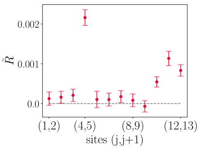
Figure 7: We estimate $\tilde{R}$ for neighbouring qubits $(j,j^{\prime})$ as $\hat{\tilde{R}}=\frac{1}{N_{I}}\sum_{i=1}^{N_{I}}\hat{\tilde{R}}^{(i)}$, where $\hat{\tilde{R}}^{(i)}=\hat{\mathcal{G}}^{(i)}_{j,j^{\prime}}-\hat{\mathcal{G}}^{(i)}_{j}\hat{\mathcal{G}}^{(i)}_{j^{\prime}}$. The error bars are estimated as the standard deviation of the mean. A value not compatible within errorbars with 0 (horizontal grey line) means that cross-talk between the qubits is present. The measurement budget is the one described in Sec. I for the calibration experiment.

D.3 Experimental investigation on the employed platform

Here, we study the locality of the noise on the platform ‘ibm_prague’ that we have used to prepare the states of interest and measure the QFI. We employ the quantity $\tilde{R}$ and estimate it using the calibration data for the 13 qubits state collected according to the indications in Sec. I. In Fig. 7 we show $\tilde{R}$ for neighbouring qubits, averaged over the iterations $i=1,\dots,N_{I}$, namely $\tilde{R}=\frac{1}{N_{I}}\sum_{i=1}^{N_{I}}\tilde{R}^{(i)}$. The error bars are estimated as the standard deviation of the mean of the different estimates. A value not compatible with 0 (horizontal grey line) witnesses the presence of cross-talk, namely $\tilde{R}\neq 0\Rightarrow\Lambda\neq\bigotimes_{i=1}^{N}\Lambda_{i}$. We observe that it is the case for the pairs of qubits $(4,5)$, $(10,11)$, $(11,12)$, $(12,13)$.

To estimate the strength of the cross-talk with respect to the local noise in the system we employ the noise model introduced in the previous section, Eq. (48) to compute $p_{\textrm{L}}^{(k)}$ and $p_{\textrm{NL}}$ from the measured values of $\tilde{G}_{j,j^{\prime}}$ and $\tilde{G}_{j}$. At first order in $p_{\textrm{NL}},p^{(k)}_{\textrm{L}}$ – in the limit $p_{\textrm{NL}},p^{(k)}_{\textrm{L}}\ll 1$ – one obtains

$$p^{(j)}_{\text{L}}\simeq\tilde{G}_{j^{\prime}}-\tilde{G}_{j,j^{\prime}},$$ (54)

$$p^{(j^{\prime})}_{\text{L}}\simeq\tilde{G}_{j}-\tilde{G}_{j,j^{\prime}},$$ (55)

$$p_{\text{NL}}\simeq\tilde{R}.$$ (56)

by inverting Eqs. (50)–(53).

pair (j,j’)	$\tilde{G}_{j}$	$\tilde{G}_{j^{\prime}}$	$\tilde{G}_{j,j^{\prime}}$	$p^{(j)}_{\text{L}}$	$p^{(j^{\prime})}_{\text{L}}$	$p_{\text{NL}}\simeq\tilde{R}$
$(1,2)$	0.9775(3)	0.9783(2)	0.9565(4)	0.0218(5)	0.0210(3)	0.0001(1)
$(2,3)$	0.9783(2)	0.9873(1)	0.9661(3)	0.0212(4)	0.0122(3)	0.0002(1)
$(3,4)$	0.9873(1)	0.9756(2)	0.9634(3)	0.0121(4)	0.0238(4)	0.0002(1)
$(4,5)$	0.9756(2)	0.9661(4)	0.9447(5)	0.0214(5)	0.0308(6)	0.0022(1)
$(5,6)$	0.9661(4)	0.9847(10)	0.9515(10)	0.0332(11)	0.0146(14)	0.0001(1)
$(6,7)$	0.9847(10)	0.9754(2)	0.9606(10)	0.0148(14)	0.0240(10)	0.0001(1)
$(7,8)$	0.9754(2)	0.9843(2)	0.9604(2)	0.0239(3)	0.0150(3)	0.0002(1)
$(8,9)$	0.9843(2)	0.9815(2)	0.9662(3)	0.0152(3)	0.0181(3)	0.0002(1)
$(9,10)$	0.9815(2)	0.9843(2)	0.9669(3)	0.0182(4)	0.0154(3)	-0.0001(1)
$(10,11)$	0.9844(2)	0.9863(2)	0.9713(3)	0.0149(4)	0.0129(5)	0.0005(1)
$(11,12)$	0.9863(2)	0.9727(3)	0.9595(3)	0.0121(4)	0.0267(5)	0.0030(1)
$(12,13)$	0.9717(3)	0.9892(1)	0.9621(3)	0.0271(4)	0.0096(4)	0.0008(1)

Table 1: Table containing the experimentally measured values of $\tilde{G}_{j}$, $\tilde{G}_{j^{\prime}}$, $\tilde{G}_{j,j^{\prime}}$ and $p_{\text{NL}}$, $p^{(k)}_{\text{L}}$ ($k=j,j^{\prime}$) calculated according to Eqs. (50)–(53) and using the estimators $\hat{\mathcal{G}}_{j}$, $\hat{\mathcal{G}}_{j,j^{\prime}}$. The number in parentheses is the numerical value of the statistical error referred to the corresponding last digits of the result.

Plugging in these equations the experimental values of $\tilde{G}_{j,j^{\prime}}$ and $\tilde{G}_{j}$ it is possible to compute the probability ratio $p_{\text{NL}}/p^{(k)}_{\text{L}}$ that is informative of the relative strength of non-local noise. Such as for $\tilde{R}$, the measured values of $\tilde{G}_{j,j^{\prime}}$ and $\tilde{G}_{j}$ are an average over the estimates of the different iterations $i=1,\dots,N_{I}$ and their error bars are calculated as the standard deviation of the mean. We employ the estimators $\hat{\mathcal{G}}_{j}$ and $\hat{\mathcal{G}}_{j,j^{\prime}}$ discussed in the main text and Sec. 45.

We give the experimental results for any pair of neighbouring qubits in Tab. 1. We observe that in the illustrative case of qubits $(4,5)$ – where $\tilde{R}=0.002$ signals the presence of non-local noise – we obtain $p_{\text{NL}}/p^{(k)}_{\text{L}}\simeq 10^{-1}$ for both $k=j,j^{\prime}$. More in general, for pairs $(4,5)$, $(11,12)$ and $(12,13)$, $p_{\text{NL}}$ is not compatible with zero within errors. However, given that $p_{\text{NL}}/p^{(k)}_{\text{L}}\lesssim 10^{-1}$ we can conclude that the amount of cross-talk error in our platform would not harm the robust shadow protocol that we employ, as investigated numerically in Ref. [38]. The dominant source of error, under the assumptions of our noise model, corresponds to local measurement errors, which can be corrected faithfully via local robust shadows.

Appendix E Further experimental results

E.1 Purity estimation of the GHZ state

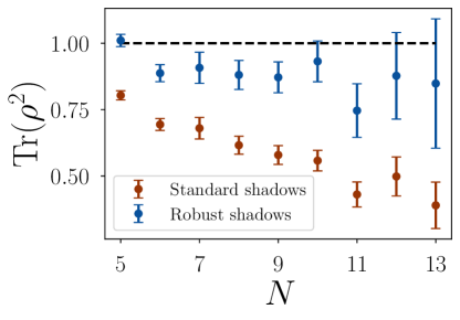
Figure 8: Purity of the GHZ state prepared on the quantum processor ‘ibm_prague’ as a function of the number of qubits. The blue points are the results obtained mitigating the error according to our protocol (robust classical shadow). The orange points correspond to unmitigated (standard classical shadow) results. The measurement budget is the one employed for every experiment and is detailed in Sec. I.

As an example of a different, important property of a quantum state $\rho$ which we can estimate with our protocol, we present here the estimation of the purity $\Tr(\rho^{2})$ of the prepared GHZ state in our hardware in Fig. 8. Similarly to the estimation of $F_{n}$, we use the U-statistics estimator from batch shadows, see Ref. [60]. We show both the mitigated (robust) and unmitigated (standard) results. Overall, we observe that increasing the number of qubits $N$ the purity of the prepared state decreases since the additional gates induce more noise in the system. However, using robust shadows, the purity decay is moderate and we can observe purities of order $0.8$ for the whole qubit range.

E.2 Ground state of the TFIM at the critical point

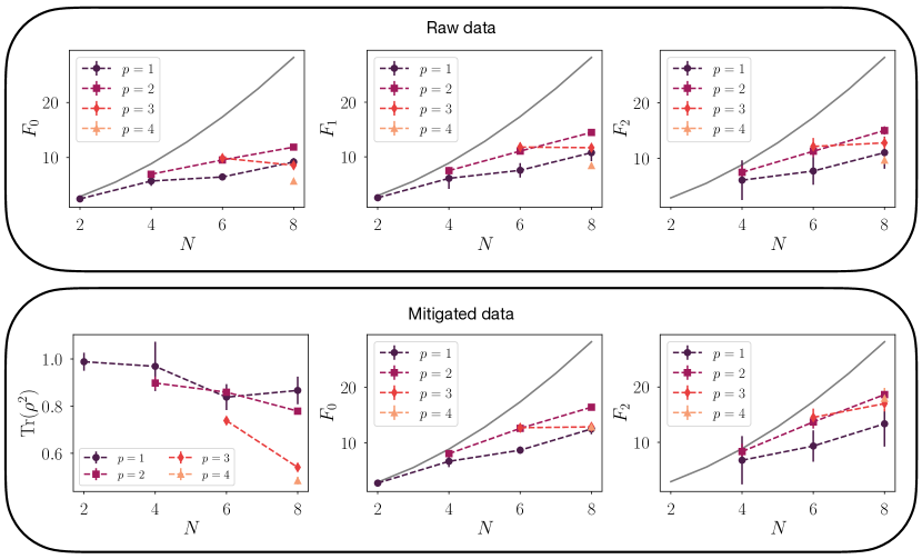
Figure 9: More experimental results on the TFIM at the critical point. In the upper panels we present results using unmitigated data for $F_{0}$, $F_{1}$, $F_{2}$. In the lower panels we use our calibration procedure for the estimation of the quantities. We show the purity $\Tr(\rho^{2})$ of the prepared state, $F_{0}$ and $F_{2}$. The results for $F_{1}$ have already been presented in the main text. The measurement protocol details are described in Sec. I. In all the plots, $p$ is the number of layers in the circuit, i.e. the depth of the circuit. The solid black lines correspond to the exact value of the QFI $F_{Q}$.

In this section we give additional experimental results concerning the ground state of the TFIM at $h=1$, prepared with the variational circuit described in the main text. We have showed explicitly the value of the bound $F_{1}$ in the case of mitigated results. In Fig. 9 we show $F_{0}$, $F_{2}$ and the purity $\Tr(\rho^{2})$ of the state in the case of raw (upper) and mitigated (lower) data. From the value of the purity we observe that increasing the number of layers in the variational circuit strongly affects the preparation of the state. The final state should be a pure state in the ideal scenario, i.e. $\Tr(\rho^{2})=1$. Here we observe that increasing the number of layers tends to decrease the purity of the prepared state, e.g. for $p=4$ and $N=8$ one has $\Tr(\rho^{2})\sim 0.5$. From the comparison of $F_{0}$ and $F_{2}$ in the two rows, we observe that they are always underestimated when no error mitigation is applied ($F_{n}$ with mitigated data is always larger than the non mitigation counterpart). This is in perfect agreement with the fact that there is noise in the measurement protocol. For completeness we also show $F_{1}$ using unmitigated data (its mitigated counterpart has been shown in the main text).

E.3 Comparison of error mitigation protocols

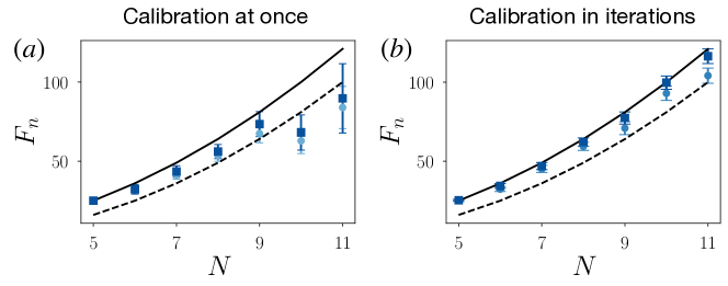
Figure 10: Comparison of of different methods of calibration. $F_{0}$ and $F_{1}$ (light to dark) when $(a)$ the calibration of the device is performed at the beginning of the whole experimental run, $(b)$ the calibration is performed in each iteration according to the experimental protocol described in the main text. The measurement budget of both experiments is the same and is detailed in Sec. I. The solid line is the exact value of the QFI ($F_{Q}=N^{2}$) for pure GHZ states. The dashed black line corresponds to the entanglement witness $\Gamma(N,k=N-1)=(N-1)^{2}$ above which the state is considered to be GME.

In this section we show experimental evidence of the effectiveness of our protocol. In Fig. 10 we compare the estimation of the bound of the QFI when the calibration of the device is performed at the beginning of the whole experimental procedure or according to our prescriptions. We present the error mitigated experimental estimations of $F_{0}$ and $F_{1}$ (light to dark). In Fig. 10$(a)$ the calibration is performed at the beginning. We observe that the robust estimation for larger system sizes is not compatible with the $\sim N^{2}$ scaling predicted by the theory, as it does not violate the witness of $(N-1)^{2}$ that validates GME. In Fig. 10$(b)$ we present the same experimental results of the main text for $F_{0}$ and $F_{1}$. As already commented, we observe the $\sim N^{2}$ scaling of QFI and witness GME. The discrepancy is due to the fluctuating gate and readout errors in the quantum processors that affect the reliability of the results when the experimental run takes long times, that is for larger $N$.

Appendix F Numerical investigations

This section aims at highlighting the behaviour of statistical errors that is caused due to finite number of measurements taken in our protocol. In particular, we study the scaling of $\hat{\mathcal{G}}_{j}$ as a function of the number of unitaries $N_{U}$ and the scaling of the required number of measurements to achieve a given level of statistical errors on our highest measured bound $F_{2}$. Lastly, we present classical numerical experiment for GHZ states prepared without any state preparation errors.

F.1 $\mathcal{G}_{j}$ as a function of the readout error

In this section, we study numerically the estimator $\hat{\mathcal{G}}_{j}$ in Eq. (32). We employ the IBM quantum simulator for providing an estimate of the scaling of $\hat{\mathcal{G}}_{j}$ as a function of the number of unitaries $N_{U}$ in the randomized measurement protocol in the calibration step. We induce noise in the circuit as a readout error $\epsilon$, since it is what mostly affects the estimation of $\hat{\mathcal{G}}_{j}$, as studied in Sec. B.3.

In Fig. 11 we observe $\hat{\mathcal{G}}_{j}$ for different $\epsilon$, as a function of $N_{U}$. The estimation is compatible with the theoretical values (dashed lines) within error bars, for any value of $\epsilon$. We observe the error bars on the estimation decreases with $N_{U}$, for fixed $N_{M}=1000$. For the value of $N_{U}$ used in our experimental protocol ($N_{U}\sim 200$) we observe an uncertainty of $\sim 1\%$ on the estimation of $\hat{\mathcal{G}}_{j}$. Increasing the number of unitaries used does not improve the estimation significantly. Hence, we choose $N_{U}=200$.

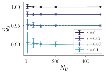
Figure 11: Numerical simulation of the calibration protocol on the IBMQ quantum simulator for a two qubit system. We plot $\hat{\mathcal{G}}_{j}$ as a function of $N_{U}$, for $N_{M}=1000$ and varying $\epsilon$ readout error.

F.2 Scaling of the measurement budget for the lower bounds

In Fig. 12, we provide numerical simulations to extract the scalings of the statistical errors on our highest measured lower bounds $F_{2}$. We consider an $N$-qubit pure GHZ state and consider the Hermitian operator $A=\frac{1}{2}\sum_{j=1}^{N}\sigma_{j}^{z}$. We simulate the protocol by applying $N_{U}$ local random unitaries $U^{(r)}$ with $r=1,\dots,N_{U}$ with $N_{M}=1000$ projective computational basis measurements per unitary to obtain batch estimates $\hat{F}_{2}$ using $N_{B}=10$ batches (c.f Eq. (8) of the main text). The average statistical error $\mathcal{E}$ is calculated by averaging the relative error ${\mathcal{E}}=|\hat{F}_{2}-F_{2}|/F_{2}$ over 100 numerically simulated experimental runs for different values of $N_{U}$. We find the maximum value of $N_{U}$ for which we obtain $\mathcal{E}\leq 0.1$ for different system sizes $N$ by using a linear interpolation function.

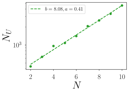
Figure 12: Numerical simulations to provide the number unitaries $N_{U}$ required to estimate $F_{2}$ below an error of $\mathcal{E}\sim 10\%$ for a GHZ state with respect to $A=\frac{1}{2}\sum_{j=1}^{N}\sigma_{j}^{z}$. We simulate $N_{M}=1000$ computational basis measurements per unitary. The dashed line are exponential fits of the type $2^{b+aN}$ highlighting the scaling as a function of the system size $N$.

F.3 Numerical simulation of the experiment

In this last section, we provide the measurement of the lower bounds via a classical numerical experiment for GHZ states prepared without any state preparation errors (perfect GHZ states). We take the same measurement budget as applied in the experimental procedure (c.f Sec. I of the main text). Additionally, we consider that the single qubit random unitary operations are done perfectly and take into account only readout errors with a probability of $p_{\rm meas}=1.4\%$ as recorded for the IBM superconducting qubit device ‘ibm_prague’ [35]. The results are shown in Fig. 13.

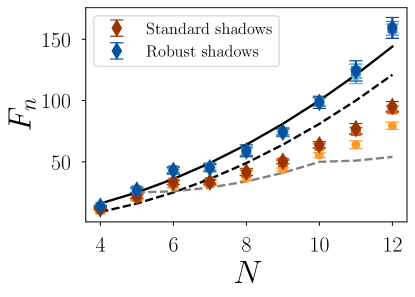
Figure 13: Numerical simulation of the experimental procedure including readout errors for GHZ states. As also mentioned in the MT, this figure shows $F_{2}$, $F_{1}$, $F_{0}$ (dark to light with diamond, square and circle respectively) as a function of the number of qubits $N$. The solid line is the exact value of the QFI $F_{Q}=N^{2}$ for pure GHZ states. The dashed black line corresponds to the entanglement witness $\Gamma(N,k=N-1)=(N-1)^{2}$. The dashed grey line corresponds to the entanglement witness $\Gamma(N,k=5)$. We fix the operator $A=\frac{1}{2}\sum_{j=1}^{N}\sigma_{j}^{z}$.

References

- Braunstein and Caves [1994a] S. L. Braunstein and C. M. Caves, Statistical distance and the geometry of quantum states, Physical Review Letters 72, 3439 (1994a).
- Tóth [2012] G. Tóth, Multipartite entanglement and high-precision metrology, Physical Review A 85, 22322 (2012).
- Hyllus et al. [2012] P. Hyllus, W. Laskowski, R. Krischek, C. Schwemmer, W. Wieczorek, H. Weinfurter, L. Pezzé, and A. Smerzi, Fisher information and multiparticle entanglement, Physical Review A 85, 22321 (2012).
- Pezzè et al. [2017] L. Pezzè, M. Gabbrielli, L. Lepori, and A. Smerzi, Multipartite entanglement in topological quantum phases, Physical Review Letters 119, 250401 (2017).
- Ren et al. [2021a] Z. Ren, W. Li, A. Smerzi, and M. Gessner, Metrological Detection of Multipartite Entanglement from Young Diagrams, Physical Review Letters 126, 80502 (2021a).
- Hauke et al. [2016] P. Hauke, M. Heyl, L. Tagliacozzo, and P. Zoller, Measuring multipartite entanglement through dynamic susceptibilities, Nature Physics 12, 778 (2016).
- Pappalardi et al. [2017] S. Pappalardi, A. Russomanno, A. Silva, and R. Fazio, Multipartite entanglement after a quantum quench, Journal of Statistical Mechanics: Theory and Experiment 2017, 053104 (2017).
- Smerzi [2012] A. Smerzi, Zeno dynamics, indistinguishability of state, and entanglement, Physical Review Letters 109, 150410 (2012).
- Braunstein et al. [1996] S. L. Braunstein, C. M. Caves, and G. J. Milburn, Generalized Uncertainty Relations: Theory, Examples, and Lorentz Invariance, Annals of Physics 247, 135 (1996).
- Braunstein and Caves [1994b] S. L. Braunstein and C. M. Caves, Statistical distance and the geometry of quantum states, Physical Review Letters 72, 3439 (1994b).
- Pezzè et al. [2018] L. Pezzè, A. Smerzi, M. K. Oberthaler, R. Schmied, and P. Treutlein, Quantum metrology with nonclassical states of atomic ensembles, Reviews of Modern Physics 90, 35005 (2018).
- Wang et al. [2014] T.-L. Wang, L.-N. Wu, W. Yang, G.-R. Jin, N. Lambert, and F. Nori, Quantum fisher information as a signature of the superradiant quantum phase transition, New Journal of Physics 16, 063039 (2014).
- Macieszczak et al. [2016] K. Macieszczak, M. Guţă, I. Lesanovsky, and J. P. Garrahan, Dynamical phase transitions as a resource for quantum enhanced metrology, Physical Review A 93, 022103 (2016).
- Katariya and Wilde [2021] V. Katariya and M. M. Wilde, Geometric distinguishability measures limit quantum channel estimation and discrimination, Quantum Information Processing 20, 78 (2021).
- Note [1] is the Pauli matrix in an arbitrary direction acting on the spin (identity operators on the other qubits are implicit).
- O’Donnell and Wright [2016] R. O’Donnell and J. Wright, Efficient quantum tomography, in STOC’16—Proceedings of the 48th Annual ACM SIGACT Symposium on Theory of Computing (ACM, New York, 2016) pp. 899–912.
- Haah et al. [2017] J. Haah, A. W. Harrow, Z. Ji, X. Wu, and N. Yu, Sample-optimal tomography of quantum states, IEEE Transactions on Information Theory 63, 5628 (2017).
- Flammia and O’Donnell [2023] S. T. Flammia and R. O’Donnell, Quantum chi-squared tomography and mutual information testing (2023), arXiv:2305.18519 .
- Monz et al. [2011a] T. Monz, P. Schindler, J. T. Barreiro, M. Chwalla, D. Nigg, W. A. Coish, M. Harlander, W. Hänsel, M. Hennrich, and R. Blatt, 14-qubit entanglement: Creation and coherence, Physical Review Letters 106, 130506 (2011a).
- Strobel et al. [2014] H. Strobel, W. Muessel, D. Linnemann, T. Zibold, D. B. Hume, L. Pezzè, A. Smerzi, and M. K. Oberthaler, Fisher information and entanglement of non-gaussian spin states, Science 345, 424 (2014).
- Barontini et al. [2015] G. Barontini, L. Hohmann, F. Haas, J. Estève, and J. Reichel, Deterministic generation of multiparticle entanglement by quantum zeno dynamics, Science 349, 1317 (2015).
- Bohnet et al. [2016] J. G. Bohnet, B. C. Sawyer, J. W. Britton, M. L. Wall, A. M. Rey, M. Foss-Feig, and J. J. Bollinger, Quantum spin dynamics and entanglement generation with hundreds of trapped ions, Science 352, 1297 (2016).
- Schmied et al. [2016] R. Schmied, J.-D. Bancal, B. Allard, M. Fadel, V. Scarani, P. Treutlein, and N. Sangouard, Bell correlations in a Bose-Einstein condensate, Science 352, 441 (2016).
- Pezzé and Smerzi [2009] L. Pezzé and A. Smerzi, Entanglement, Nonlinear Dynamics, and the Heisenberg Limit, Physical Review Letters 102, 100401 (2009).
- Yu et al. [2022] M. Yu, Y. Liu, P. Yang, M. Gong, Q. Cao, S. Zhang, H. Liu, M. Heyl, T. Ozawa, N. Goldman, et al., Quantum fisher information measurement and verification of the quantum cramér–rao bound in a solid-state qubit, npj Quantum Information 8, 56 (2022).
- Yu et al. [2021a] M. Yu, D. Li, J. Wang, Y. Chu, P. Yang, M. Gong, N. Goldman, and J. Cai, Experimental estimation of the quantum fisher information from randomized measurements, Phys. Rev. Res. 3, 043122 (2021a).
- Rivas and Luis [2008] A. Rivas and A. Luis, Intrinsic metrological resolution as a distance measure and nonclassical light, Physical Review A 77, 063813 (2008).
- Rivas and Luis [2010] A. Rivas and A. Luis, Precision quantum metrology and nonclassicality in linear and nonlinear detection schemes, Physical Review Letters 105, 010403 (2010).
- Zhang et al. [2017] C. Zhang, B. Yadin, Z.-B. Hou, H. Cao, B.-H. Liu, Y.-F. Huang, R. Maity, V. Vedral, C.-F. Li, G.-C. Guo, and D. Girolami, Detecting metrologically useful asymmetry and entanglement by a few local measurements, Physical Review A 96, 042327 (2017).
- Girolami and Yadin [2017] D. Girolami and B. Yadin, Witnessing Multipartite Entanglement by Detecting Asymmetry, Entropy 19, 124 (2017).
- Beckey et al. [2022a] J. L. Beckey, M. Cerezo, A. Sone, and P. J. Coles, Variational quantum algorithm for estimating the quantum fisher information, Phys. Rev. Res. 4, 013083 (2022a).
- Cerezo et al. [2021a] M. Cerezo, A. Sone, J. L. Beckey, and P. J. Coles, Sub-quantum Fisher information, Quantum Science and Technology 6, 035008 (2021a).
- Ren et al. [2021b] Z. Ren, W. Li, A. Smerzi, and M. Gessner, Metrological detection of multipartite entanglement from young diagrams, Physical Review Letters 126, 080502 (2021b).
- Rath et al. [2021a] A. Rath, C. Branciard, A. Minguzzi, and B. Vermersch, Quantum fisher information from randomized measurements, Physical Review Letters 127, 260501 (2021a).
- IBM-Quantum [2021] IBM-Quantum, https://quantum-computing.ibm.com/ (2021).
- Elben et al. [2023] A. Elben, S. T. Flammia, H.-Y. Huang, R. Kueng, J. Preskill, B. Vermersch, and P. Zoller, The randomized measurement toolbox, Nature Reviews Physics 5, 9 (2023).
- Farhi et al. [2014] E. Farhi, J. Goldstone, and S. Gutmann, A quantum approximate optimization algorithm (2014), arXiv:1411.4028 .
- Chen et al. [2021] S. Chen, W. Yu, P. Zeng, and S. T. Flammia, Robust shadow estimation, PRX Quantum 2, 030348 (2021).
- Koh and Grewal [2022] D. E. Koh and S. Grewal, Classical shadows with noise, Quantum 6, 776 (2022).
- Mezzadri [2007] F. Mezzadri, How to generate random matrices from the classical compact groups (2007), arXiv:math-ph/0609050 .
- Note [2] One can also implement different unitaries for calibration and estimation. For the present experiment, we did not notice significant differences as we estimate different quantities.
- Brydges et al. [2019] T. Brydges, A. Elben, P. Jurcevic, B. Vermersch, C. Maier, B. P. Lanyon, P. Zoller, R. Blatt, and C. F. Roos, Probing Rényi entanglement entropy via randomized measurements, Science 364, 260 (2019).
- Rath et al. [2021b] A. Rath, R. van Bijnen, A. Elben, P. Zoller, and B. Vermersch, Importance sampling of randomized measurements for probing entanglement, Physical Review Letters 127, 200503 (2021b).
- Satzinger et al. [2021] K. J. Satzinger, Y.-J. Liu, A. Smith, C. Knapp, M. Newman, C. Jones, Z. Chen, C. Quintana, X. Mi, A. Dunsworth, C. Gidney, I. Aleiner, F. Arute, K. Arya, J. Atalaya, Babbush, et al., Realizing topologically ordered states on a quantum processor, Science 374, 1237 (2021).
- Yu et al. [2021b] X.-D. Yu, S. Imai, and O. Gühne, Optimal entanglement certification from moments of the partial transpose, Physical Review Letters 127, 060504 (2021b).
- Vitale et al. [2022] V. Vitale, A. Elben, R. Kueng, A. Neven, J. Carrasco, B. Kraus, P. Zoller, P. Calabrese, B. Vermersch, and M. Dalmonte, Symmetry-resolved dynamical purification in synthetic quantum matter, SciPost Physics 12, 106 (2022).
- Hoke et al. [2023] J. C. Hoke, M. Ippoliti, D. Abanin, R. Acharya, M. Ansmann, F. Arute, K. Arya, A. Asfaw, J. Atalaya, J. C. Bardin, et al., Quantum information phases in space-time: measurement-induced entanglement and teleportation on a noisy quantum processor (2023), arXiv:2303.04792 .
- Elben et al. [2020a] A. Elben, R. Kueng, H.-Y. R. Huang, R. van Bijnen, C. Kokail, M. Dalmonte, P. Calabrese, B. Kraus, J. Preskill, P. Zoller, and B. Vermersch, Mixed-State Entanglement from Local Randomized Measurements, Physical Review Letters 125, 200501 (2020a).
- Neven et al. [2021] A. Neven, J. Carrasco, V. Vitale, C. Kokail, A. Elben, M. Dalmonte, P. Calabrese, P. Zoller, B. Vermersch, R. Kueng, and B. Kraus, Symmetry-resolved entanglement detection using partial transpose moments, npj Quantum Information 7, 152 (2021).
- Carrasco et al. [2022] J. Carrasco, M. Votto, V. Vitale, C. Kokail, A. Neven, P. Zoller, B. Vermersch, and B. Kraus, Entanglement phase diagrams from partial transpose moments (2022), arXiv:2212.10181 .
- Elben et al. [2020b] A. Elben, B. Vermersch, R. Van Bijnen, C. Kokail, T. Brydges, C. Maier, M. K. Joshi, R. Blatt, C. F. Roos, and P. Zoller, Cross-Platform Verification of Intermediate Scale Quantum Devices, Physical Review Letters 124, 10504 (2020b).
- Zhu et al. [2022] D. Zhu, Z. P. Cian, C. Noel, A. Risinger, D. Biswas, L. Egan, Y. Zhu, A. M. Green, C. H. Alderete, N. H. Nguyen, Q. Wang, A. Maksymov, Y. Nam, M. Cetina, N. M. Linke, M. Hafezi, and C. Monroe, Cross-platform comparison of arbitrary quantum states, Nature Communications 13, 6620 (2022).
- Joshi et al. [2023] M. K. Joshi, C. Kokail, R. van Bijnen, F. Kranzl, T. V. Zache, R. Blatt, C. F. Roos, and P. Zoller, Exploring large-scale entanglement in quantum simulation (2023), arXiv:2306.00057 .
- Joshi et al. [2020] M. K. Joshi, A. Elben, B. Vermersch, T. Brydges, C. Maier, P. Zoller, R. Blatt, and C. F. Roos, Quantum information scrambling in a trapped-ion quantum simulator with tunable range interactions, Physical Review Letters 124, 240505 (2020).
- Cian et al. [2021] Z.-P. Cian, H. Dehghani, A. Elben, B. Vermersch, G. Zhu, M. Barkeshli, P. Zoller, and M. Hafezi, Many-body chern number from statistical correlations of randomized measurements, Physical Review Letters 126, 050501 (2021).
- Elben et al. [2020c] A. Elben, J. Yu, G. Zhu, M. Hafezi, F. Pollmann, P. Zoller, and B. Vermersch, Many-body topological invariants from randomized measurements in synthetic quantum matter, Science Advances 6, eaaz3666 (2020c).
- Cieśliński et al. [2023] P. Cieśliński, S. Imai, J. Dziewior, O. Gühne, L. Knips, W. Laskowski, J. Meinecke, T. Paterek, and T. Vértesi, Analysing quantum systems with randomised measurements (2023), arXiv:2307.01251 .
- Huang et al. [2020] H.-Y. Huang, R. Kueng, and J. Preskill, Predicting many properties of a quantum system from very few measurements, Nature Physics 16, 1050 (2020).
- Vermersch et al. [2023] B. Vermersch, A. Rath, B. Sundar, C. Branciard, J. Preskill, and A. Elben, Enhanced estimation of quantum properties with common randomized measurements (2023), arXiv:2304.12292 .
- Rath et al. [2023] A. Rath, V. Vitale, S. Murciano, M. Votto, J. Dubail, R. Kueng, C. Branciard, P. Calabrese, and B. Vermersch, Entanglement barrier and its symmetry resolution: Theory and experimental observation, PRX Quantum 4, 010318 (2023).
- Hoeffding [1992] W. Hoeffding, A class of statistics with asymptotically normal distribution, in Breakthroughs in Statistics (Springer, 1992) pp. 308–334.
- Boschi et al. [1998] D. Boschi, S. Branca, F. De Martini, L. Hardy, and S. Popescu, Experimental realization of teleporting an unknown pure quantum state via dual classical and einstein-podolsky-rosen channels, Physical Review Letters 80, 1121 (1998).
- Bouwmeester et al. [1997] D. Bouwmeester, J.-W. Pan, K. Mattle, M. Eibl, H. Weinfurter, and A. Zeilinger, Experimental quantum teleportation, Nature 390, 575 (1997).
- Gottesman and Chuang [1999] D. Gottesman and I. L. Chuang, Demonstrating the viability of universal quantum computation using teleportation and single-qubit operations, Nature 402, 390 (1999).
- Knill et al. [1998] E. Knill, R. Laflamme, and W. H. Zurek, Resilient quantum computation, Science 279, 342 (1998).
- Bennett et al. [1992] C. H. Bennett, G. Brassard, and N. D. Mermin, Quantum cryptography without Bell’s theorem, Physical Review Letters 68, 557 (1992).
- Giovannetti et al. [2006] V. Giovannetti, S. Lloyd, and L. Maccone, Quantum metrology, Physical Review Letters 96, 010401 (2006).
- Tóth and Apellaniz [2014] G. Tóth and I. Apellaniz, Quantum metrology from a quantum information science perspective, Journal of Physics A: Mathematical and Theoretical 47, 424006 (2014).
- Song et al. [2017] C. Song, K. Xu, W. Liu, C.-p. Yang, S.-B. Zheng, H. Deng, Q. Xie, K. Huang, Q. Guo, L. Zhang, P. Zhang, D. Xu, D. Zheng, X. Zhu, H. Wang, Y.-A. Chen, C.-Y. Lu, S. Han, and J.-W. Pan, 10-qubit entanglement and parallel logic operations with a superconducting circuit, Phys. Rev. Lett. 119, 180511 (2017).
- Mooney et al. [2021] G. J. Mooney, G. A. L. White, C. D. Hill, and L. C. L. Hollenberg, Generation and verification of 27-qubit greenberger-horne-zeilinger states in a superconducting quantum computer, Journal of Physics Communications 5, 095004 (2021).
- Monz et al. [2011b] T. Monz, P. Schindler, J. T. Barreiro, M. Chwalla, D. Nigg, W. A. Coish, M. Harlander, W. Hänsel, M. Hennrich, and R. Blatt, 14-qubit entanglement: Creation and coherence, Phys. Rev. Lett. 106, 130506 (2011b).
- Wang et al. [2018] X.-L. Wang, Y.-H. Luo, H.-L. Huang, M.-C. Chen, Z.-E. Su, C. Liu, C. Chen, W. Li, Y.-Q. Fang, X. Jiang, J. Zhang, L. Li, N.-L. Liu, C.-Y. Lu, and J.-W. Pan, 18-qubit entanglement with six photons’ three degrees of freedom, Phys. Rev. Lett. 120, 260502 (2018).
- Song et al. [2019] C. Song, K. Xu, H. Li, Y.-R. Zhang, X. Zhang, W. Liu, Q. Guo, Z. Wang, W. Ren, J. Hao, H. Feng, H. Fan, D. Zheng, D.-W. Wang, H. Wang, and S.-Y. Zhu, Generation of multicomponent atomic schrödinger cat states of up to 20 qubits, Science 365, 574 (2019).
- Gong et al. [2019] M. Gong, M.-C. Chen, Y. Zheng, S. Wang, C. Zha, H. Deng, Z. Yan, H. Rong, Y. Wu, S. Li, F. Chen, Y. Zhao, F. Liang, J. Lin, Y. Xu, C. Guo, L. Sun, A. D. Castellano, H. Wang, C. Peng, C.-Y. Lu, X. Zhu, and J.-W. Pan, Genuine 12-qubit entanglement on a superconducting quantum processor, Phys. Rev. Lett. 122, 110501 (2019).
- Pogorelov et al. [2021] I. Pogorelov, T. Feldker, C. D. Marciniak, L. Postler, G. Jacob, O. Krieglsteiner, V. Podlesnic, M. Meth, V. Negnevitsky, M. Stadler, B. Höfer, C. Wächter, K. Lakhmanskiy, R. Blatt, P. Schindler, and T. Monz, Compact ion-trap quantum computing demonstrator, PRX Quantum 2, 020343 (2021).
- Cao et al. [2023] S. Cao, B. Wu, F. Chen, M. Gong, Y. Wu, Y. Ye, C. Zha, H. Qian, C. Ying, S. Guo, Q. Zhu, H.-L. Huang, Y. Zhao, S. Li, S. Wang, J. Yu, D. Fan, D. Wu, H. Su, H. Deng, H. Rong, Y. Li, K. Zhang, T.-H. Chung, F. Liang, J. Lin, Y. Xu, L. Sun, C. Guo, N. Li, Y.-H. Huo, C.-Z. Peng, C.-Y. Lu, X. Yuan, X. Zhu, and J.-W. Pan, Generation of genuine entanglement up to 51 superconducting qubits, Nature 619, 738 (2023).
- Omran et al. [2019] A. Omran, H. Levine, A. Keesling, G. Semeghini, T. T. Wang, S. Ebadi, H. Bernien, A. S. Zibrov, H. Pichler, S. Choi, et al., Generation and manipulation of schrödinger cat states in rydberg atom arrays, Science 365, 570 (2019).
- Wei et al. [2020] K. X. Wei, I. Lauer, S. Srinivasan, N. Sundaresan, D. T. McClure, D. Toyli, D. C. McKay, J. M. Gambetta, and S. Sheldon, Verifying multipartite entangled greenberger-horne-zeilinger states via multiple quantum coherences, Physical Review A 101, 032343 (2020).
- Gabbrielli et al. [2018] M. Gabbrielli, A. Smerzi, and L. Pezzè, Multipartite Entanglement at Finite Temperature, Scientific Reports 8, 15663 (2018).
- Frérot and Roscilde [2018] I. Frérot and T. Roscilde, Quantum critical metrology, Physical review letters 121, 020402 (2018).
- Koczor et al. [2020] B. Koczor, S. Endo, T. Jones, Y. Matsuzaki, and S. C. Benjamin, Variational-state quantum metrology, New Journal of Physics 22, 083038 (2020).
- Cerezo et al. [2021b] M. Cerezo, A. Arrasmith, R. Babbush, S. C. Benjamin, S. Endo, K. Fujii, J. R. McClean, K. Mitarai, X. Yuan, L. Cincio, and P. J. Coles, Variational quantum algorithms, Nature Reviews Physics 3, 625 (2021b).
- Beckey et al. [2022b] J. L. Beckey, M. Cerezo, A. Sone, and P. J. Coles, Variational quantum algorithm for estimating the quantum fisher information, Physical Review Research 4, 013083 (2022b).
- Ho and Hsieh [2019] W. W. Ho and T. H. Hsieh, Efficient variational simulation of non-trivial quantum states, SciPost Phys. 6, 029 (2019).
- Hempel et al. [2018] C. Hempel, C. Maier, J. Romero, J. McClean, T. Monz, H. Shen, P. Jurcevic, B. P. Lanyon, P. Love, R. Babbush, A. Aspuru-Guzik, R. Blatt, and C. F. Roos, Quantum chemistry calculations on a trapped-ion quantum simulator, Physical Review X 8, 031022 (2018).
- Huang et al. [2021] H.-Y. Huang, R. Kueng, and J. Preskill, Efficient estimation of pauli observables by derandomization, Physical Review Letters 127, 030503 (2021).
- Huang et al. [2022] H.-Y. Huang, R. Kueng, G. Torlai, V. V. Albert, and J. Preskill, Provably efficient machine learning for quantum many-body problems, Science 377, eabk3333 (2022).
- Lewis et al. [2023] L. Lewis, H.-Y. Huang, V. T. Tran, S. Lehner, R. Kueng, and J. Preskill, Improved machine learning algorithm for predicting ground state properties (2023), arXiv:2301.13169 .
- Johansson et al. [2013] J. Johansson, P. Nation, and F. Nori, QuTiP 2: A Python framework for the dynamics of open quantum systems, Computer Physics Communications 184, 1234 (2013).
- Elben et al. [2019] A. Elben, B. Vermersch, C. F. Roos, and P. Zoller, Statistical correlations between locally randomized measurements: A toolbox for probing entanglement in many-body quantum states, Physical Review A 99, 052323 (2019).
- Baheri et al. [2022] B. Baheri, Q. Guan, V. Chaudhary, and A. Li, Quantum noise in the flow of time: A temporal study of the noise in quantum computers, in 2022 IEEE 28th International Symposium on On-Line Testing and Robust System Design (IOLTS) (2022) pp. 1–5.
- Hirasaki et al. [2023] Y. Hirasaki, S. Daimon, T. Itoko, N. Kanazawa, and E. Saitoh, Detection of temporal fluctuation in superconducting qubits for quantum error mitigation (2023), arXiv:2307.04337 .