Quantum coherent and measurement feedback control based on atoms coupled with a semi-infinite waveguide

Abstract

In this paper, we show that quantum feedback control may be applied to generate desired states for atomic and photonic systems based on a semi-infinite waveguide coupled with multiple two-level atoms. In this set-up, an initially excited atom can emit one photon into the waveguide, which can be reflected by the terminal mirror or other atoms to establish different feedback loops via the coherent interactions between the atom and photon. When there are at most two excitations in the waveguide quantum electrodynamics (waveguide QED) system, the evolution of quantum states can be interpreted using random graph theory. While this process is influenced by the environment, and we clarify that the environment-induced dynamics can be eliminated by measurement-based feedback control or coherent drives. Thus, in the open system atom-waveguide interactions, measurement-based feedback can modulate the final steady quantum state, while simultaneously, the homodyne detection noise in the measurement process can induce oscillations, which is treated by the coherent feedback designs.

81Q93, 81S25, 93B52, 93C43

1 Introduction

Quantum feedback control has attracted much attention for its applications in quantum information processing (QIP) [1, 2], quantum optics [3, 1, 4], and quantum metrology [5, 6, 7]. Depending on whether or not the measurement results of the quantum state are used in the feedback control laws, quantum feedback can be divided into measurement-based and coherent quantum feedback, respectively. In the coherent feedback design, the quantum components can be directly coupled with another quantum component working as a controller [2], then the system and controller evolve unitarily. For example, in quantum control based on continuous variable system, the optical nonlinear crystal can be manipulated by the pump field, while the output field can be made to re-interact with the crystal by reflecting it back using mirrors, thereby setting up a quantum coherent feedback loop. The dynamics of the optical crystal is then controlled by the pump filed and coherent feedback field [8]. This coherent feedback process can never induce backaction noise into the quantum system and the feedback loop length is tunable, which can be an ideal platform for generating optical entangled states. In contrast, measurement-based quantum feedback control uses the results of measurement of the quantum system so that we deal with the non-linear conditioned evolution of the quantum state. For example, in quantum error correction with the encoded three-qubit bit-flip code, quantum states with evolution errors can be detected via the continuous measurement evaluated by the current, then appropriate feedback action can be applied to each qubit to correct the operation errors [9]. Both of the feedback schemes have various realization formats in practical systems, and it is meaningful to explore their dynamics from the perspective of control theory.

Quantum coherent feedback control can be realized through interactions among the atom, cavity, waveguide, etc. For example, two cavities may be coupled via a semi-transparent mirror so that, if there is an excited atom in one of the cavities, then the excited atom can emit a coherent field (i.e., a photon) which is then transmitted into the other cavity through the semi-transparent mirror and eventually re-interact with the atom in the former cavity thereby constructing a quantum coherent feedback loop [10, 11, 12]. More generally, a cavity containing one or more atoms can also be coupled with a semi-infinite waveguide with continuous modes, and the photons in the cavity can leak into the waveguide and re-interact with cavity-QED system after transmission and reflection in the waveguide [13]. Then the dynamics of the cavity-QED system (i.e., the atomic states and the number of photons) can be modified by the properties of the coherent feedback loop such as the length of the waveguide or the coupling strength between the cavity and waveguide. Alternatively, an atom may be directly coupled with the waveguide without the mediation of the cavity: the simplest case is a two-level atom coupled with a semi-infinite waveguide, where the excited atom can emit one photon into the waveguide, and the transmitted photon wave packet can be reflected by the terminal mirror at one end of the waveguide, which is then reflected and reabsorbed by the atom. The emission and reflection of the photon sets up a coherent feedback loop and the dynamics is dependent on the coupling strength between the atom and the waveguide, and the distance between the atom and the terminal mirror. When there are multiple atoms coupled with the waveguide, the photon emitted by one atom can be absorbed and re-emitted by another atom after being transmitted in the waveguide, and the photon’s transmission between two atoms can construct a coherent feedback loop [14]. The dynamical complexity of coherent feedback control increases with the adding of the number of excitations and emitters, and is also influenced by the feedback loop length and the chiral couplings between the atom and the waveguide [15, 16, 17, 18]. For example, chiral couplings between the atom and waveguide can control the propagation direction of the emitted photon wave packet in the waveguide [18]. For the one-excitation system where there are two two-level atoms coupled with a semi-infinite waveguide, the coherent feedback dynamics can induce entanglement between the two atoms [19]. For the coherent feedback network with two excitations, the generation of two-photon states may depend on the feedback loop length, i.e., the length of the waveguide coupled with the cavity-QED system [20], or the locations of the two-atom network coupled with a semi-infinite waveguide [18]. When there are multiple atoms coupled with an infinite waveguide, the entanglement between arbitrary two atoms can be modulated by tuning the locations of atoms and their chiral coupling strengths with the waveguide [21].

In the quantum measurement feedback control, the measurement information of the quantum state can be used to remodulate the quantum system [1]. Taking a one-bit toy model in quantum computation as an example [9], the random bit-flip error has the effect of reversing the encoded qubit’s value, then the state of the qubit can be measured according to the current with the given measurement rate, and finally the feedback control can drive a qubit to the desired state. During this process, quantum measurements can introduce random noise to the current value, and the quantum system dynamics should be modeled with the stochastic master equation [22]. The closed-loop control of the qubit is determined by the measurement and feedback strengths, the detector efficiency, etc., and can be optimized by tuning the smoothing filter for the measurement results [9, 23]. A more widely used scheme is the three-qubit bit-flip code for quantum error correction [9, 24, 25], where the measurement feedback control generalized from the one-qubit case can detect and correct not only a single bit-flip error, but also the double flipping error events. Quantum measurement feedback control is also helpful for the generation of entanglement between qubits, especially for the enhancement of success rate and fidelity [26, 27]. As proposed in Ref. [28], the feedback Hamiltonian designed according to the weak measurement can guide the quantum system to the decoherence-free subspace, and this can further influence the strength of bipartite entanglement. Additionally, in the open quantum system with relaxation and dephasing effects, the designed measurement feedback can preserve the quantum system’s coherence, i.e., the coherence between the ground and excited state of a single qubit [29].

The measurement of the quantum state can be designated as quantum non-demolition (QND) measurement and non-QND measurement depending on whether or not the measurement operator commutes with the quantum system Hamiltonian [30, 31, 32, 33]. For example, in the early realization of photon QND measurement based on the cavity-QED system, the atom acting as a meter can interact with the cavity by absorbing and emitting a photon if initially there is one photon in the cavity, and then the existence of photons in the cavity can be inferred by detecting the phase shift of the atom [34]. In this process, the atom meter does not annihilate the photon in the cavity, and it can further be used to stabilize the photon number in the cavity [35]. However, when the measurement operator dose not commute with the system Hamiltonian, theoretically the steady value will be different and some eigenstates of the system Hamiltonian cannot be generated no matter how the control fields are utilized [31]. Non-QND measurement can be realized in the setting of waveguide QED where atoms are coupled with an infinite or semi-infinite waveguide [36, 37, 38, 39, 40, 41, 42], and homodyne detection or photon counting at the output end of the waveguide according to the atomic lowering operator. Similarly with the cavity-QED system, the homodyne detection results can be used to design the feedback control fields for the waveguide QED system, and this feedback dynamics based on non-QND measurement has not been systematically explored.

In this paper, we study the feedback dynamics for an assembly of two-level atoms coupled via a semi-infinite waveguide, then both coherent feedback and measurement feedback can influence the atomic states. Generalizing from the two-atom case in Ref. [18], we first consider the coherent feedback in the closed quantum system based on multiple two-level atoms coupled with a semi-infinite waveguide, and then subsequently study the dynamics influenced by the environment in the open system. Taking the case that a single two-level atom coupled with the waveugide in the open quantum system as an example, the decay and dissipation of the quantum system due to the environment can prevent the atom from being ideally excited as in the closed system. On the one hand, with the help of external coherent drives or measurement feedback controls, the atom can be excited rather than decay to the ground state. On the other hand, the measurement process with homodyne detection noises can control the atomic dynamics, and this is related to the coherent feedback designs.

The paper is organized as follows. In Section 2, we investigate the coherent feedback control in the closed system based on the architecture of multiple two-level atoms coupled with a semi-infinite waveguide. Here,the evolution of the quantum states can be best described using ideas from random graph theory. In Section 3 we study on the combination of coherent feedback control and measurement feedback control in the open system based on the set up where one two-level atom is coupled with a semi-infinite waveguide. With the help of external coherent drives and measurement feedback control fields, we can also modulate the quantum state. We present our conclusions in Section 4.

2 Coherent feedback control with one or two excitations

Figure 1: (a) Feedback control setup with $N$ two-level atoms coupled with a semi-infinite waveguide. (b) Random graph with $N$ nodes.

As in Fig. 1 (a), there are $N$ two-level atoms coupled with the semi-infinite waveguide with a perfect reflecting mirror at $z=0$, and the distance between the mirror and the $j$th atom with the resonant frequency $\omega_{aj}$ is $z_{j}$. The coupling strengths between the $j$th atom and the right/left propagating fields in the waveguide are $\gamma_{jR}$ and $\gamma_{jL}$, respectively. The interaction Hamiltonian between the $j$th atom and the waveguide is

(1) $$H_{I}^{(j)} =\int\mathrm{d}k\left[g_{kjt}(k,t,z)d^{{\dagger}}_{k}\sigma_{j}^{-}+g_{kjt}^{*}(k,t,z)d_{k}\sigma_{j}^{+}\right],$$

where $d_{k}$($d^{{\dagger}}_{k}$) are the annihilation (creation) operators of the propagating waveguide mode $k$, $\sigma_{j}^{-}=|g_{j}\rangle\langle e_{j}|$ and $\sigma_{j}^{+}=|e_{j}\rangle\langle g_{j}|$ are the lowering and raising operators of the $j$th atom, the coupling strength $g_{kjt}$ between the $j$th atom and the waveguide reads

(2) $$g_{kjt}(k,t,z) =i\left(\gamma_{jR}e^{-i\omega_{k}z_{j}/c}-\gamma_{jL}e^{i\omega_{k}z_{j}/c}\right)e^{i(\omega_{k}-\omega_{aj})t}$$

$$=i\gamma_{jR}e^{i\left[(\omega_{k}-\omega_{aj})t-\omega_{k}z_{j}/c\right]}-i\gamma_{jL}e^{i\left[(\omega_{k}-\omega_{aj})t+\omega_{k}z_{j}/c\right]},$$

where $\omega_{k}=kc$ and $c$ is the speed of light in the waveguide.

When the coupling between the atom and the waveguide is nonchiral, that is $\gamma_{jR}=\gamma_{jL}=\gamma_{j}$, the coupling can be simplified to be $g_{kjt}=2\gamma_{j}\sin(kz_{j})e^{i(\omega_{k}-\omega_{aj})t}$. The output of the waveguide can be measured with a photon detector via the homodyne detection with the collapse operator $\sigma_{j}^{-}$ at the right end of the waveguide [36, 43]. In this section, we restrict to coherent feedback schemes without the measurement process. We will explore how the measurement feedback can control the atomic dynamics in the subsequent section.

The total Hamiltonian for the atoms and the waveguide then reads

(3) $$H= \sum_{j=1}^{N}\omega_{aj}\sigma_{j}^{+}\sigma_{j}^{-}+\int_{0}^{\infty}\mathrm{d}k\omega_{k}d^{{\dagger}}_{k}d_{k}$$

$$+\sum_{j=1}^{N}\int\mathrm{d}k\left[g_{kjt}(k,t,z_{j})d^{{\dagger}}_{k}\sigma_{j}^{-}+g_{kjt}^{*}(k,t,z_{j})d_{k}\sigma_{j}^{+}\right].$$

Assumption 1.

In the system in Fig. 1 (a), there are at most two excitations in the waveguide without any additional inputs. The atoms have the same resonant frequency as $\omega_{a1}=\omega_{a2}=\cdots=\omega_{aN}=\omega_{a}$.

Based on Assumption 1, the populations of eigenstates of the quantum system in Fig. 1 (a) can be represented in terms of the evolution of the random graph in Fig. 1 (b). For example, when there is only one excitation in the quantum network, the probability representing that $j$th atom is excited can be interpreted as the probability of the $j$th vertex of the random graph. When there are overall two excitations, the probability that two atoms (i.e., the $j$th and $l$th atoms) are simultaneously excited can be interpreted as the probability of the edge connecting the $j$th and $l$th vertexes on the random graph; the probability that only the $j$th atom is excited and there is one photon in the waveguide can be interpreted as the probability of the $j$th vertex. Moreover, the quantum state that all the atoms are at the ground state can be interpreted as the complementary set of the random graph.

2.1 Coherent feedback control with one excitation

When there is at most one excitation in the $N$ two-level atom network coupled with a semi-infinite waveguide, the quantum state can be represented as:

(4) $$|\Psi(t)\rangle= \sum_{j=1}^{N}c_{j}(t)|g_{1},g_{2},\cdots,g_{j-1},e_{j},g_{j+1},\cdots,g_{N},\{0\}\rangle$$

$$+\int\tilde{c}(t,k)|g_{1},\cdots,g_{N},\{k\}\rangle\mathrm{d}k,$$

where the first component describes the state where one atom (the $j$th, for $j=1,2,\cdots,N$) is excited with no photons in the waveguide, and the second component represents that all the atoms are at the ground state and there is one photon in the waveguide. We assume initially only the first atom is excited and there are no photons in the waveguide.

Remark 2.1.

For the closed loop quantum system with feedback in Fig. 1 (a) with one excitation, the $j$th vertex on the random graph in Fig. 1 (b) with probability $p_{j}$ represents the probability that the $j$th two-level atom is excited, namely $p_{j}=|c_{j}|^{2}$ with $\sum_{j}^{N}p_{j}\leq 1$.

The dynamics of the quantum state is governed by the Schrödinger equation

$$\frac{\mathrm{d}}{\mathrm{d}t}|\Psi(t)\rangle=-iH|\Psi(t)\rangle.$$

Based on Assumption 1, the evolution of the amplitudes is given by

(5a) $$\dot{c}_{j}(t)=\int\left[-\gamma_{jR}e^{-i[(\omega_{k}-\omega_{a})t-\omega_{k}z_{j}/c]}+\gamma_{jL}e^{-i[(\omega_{k}-\omega_{a})t+\omega_{k}z_{j}/c]}\right]\tilde{c}(t,k)\mathrm{d}k,$$

(5b) $$\dot{\tilde{c}}(t,k)=\sum_{j=1}^{N}c_{j}(t)\left[\gamma_{jR}e^{i[(\omega_{k}-\omega_{a})t-\omega_{k}z_{j}/c]}-\gamma_{jL}e^{i[(\omega_{k}-\omega_{a})t+\omega_{k}z_{j}/c]}\right],$$

where Eq. (5a) means that the $j$th atom initially at the ground state can absorb one photon from the waveguide and finally can be excited, Eq. (5b) means that each excited two-level atom can emit one photon into the waveugide via the spontaneous emission. Both coefficients are influenced by the locations of atoms and the chiral coupling strengths. According to the calculations in Appendix A, Eq. (5) can be rewritten in the format of a delay dependent ODE as

(6) $$\dot{c}_{j}(t)=-\frac{\gamma_{jR}^{2}+\gamma_{jL}^{2}}{2}c_{j}(t)-\gamma_{jR}\sum_{p=1}^{j-1}\gamma_{pR}c_{p}\left(t-\frac{z_{j}-z_{p}}{c}\right)e^{i\omega_{a}\frac{z_{j}-z_{p}}{c}}$$

$$-\gamma_{jL}\sum_{p=j+1}^{N}\gamma_{pL}c_{p}\left(t-\frac{z_{p}-z_{j}}{c}\right)e^{i\omega_{a}\frac{z_{p}-z_{j}}{c}}+\gamma_{jR}\sum_{p=1}^{N}\gamma_{pL}c_{p}\left(t-\frac{z_{p}+z_{j}}{c}\right)e^{i\omega_{a}\frac{z_{p}+z_{j}}{c}},$$

where the first component of RHS of Eq. (6) means that the atom can decay to the ground state by emitting a photon along the right and left directions, the second component represents that the excited state can be transferred from the $p$th to the $j$th atom along the right direction with a delay determined by the distance between two atoms, similarly for the left direction in the third component, and the fourth component represents the transmission of the excited state after the reflection by the mirror with a round trip delay.

2.1.1 Feedback network with single delay

For the simplified circumstance that $z_{1}=z_{2}=\cdots=z_{N}$, denote

$$x(t)=\left[c_{1}(t),c_{2}(t),\cdots,c_{N}(t)\right]^{\mathrm{T}}$$

with $\mathrm{T}$ for the transpose matrix, then Eq. (5) can be rewritten as

(7) $$\dot{x}(t) =\begin{bmatrix}-\frac{\gamma_{1R}^{2}+\gamma_{1L}^{2}}{2}&-\gamma_{1L}\gamma_{2L}&-\gamma_{1L}\gamma_{3L}&\cdots&-\gamma_{1L}\gamma_{NL}\\ -\gamma_{1R}\gamma_{2R}&-\frac{\gamma_{2R}^{2}+\gamma_{2L}^{2}}{2}&-\gamma_{2L}\gamma_{3L}&\cdots&-\gamma_{2L}\gamma_{NL}\\ \vdots&\vdots&\vdots&\ddots&\vdots\\ -\gamma_{1R}\gamma_{NR}&-\gamma_{2R}\gamma_{NR}&-\gamma_{3R}\gamma_{NR}&\cdots&-\frac{\gamma_{NR}^{2}+\gamma_{NL}^{2}}{2}\end{bmatrix}x(t)$$

$$~{}~{}~{}~{}+e^{i\omega_{a}\tau}\begin{bmatrix}\gamma_{1R}\\ \gamma_{2R}\\ \vdots\\ \gamma_{NR}\end{bmatrix}\begin{bmatrix}\gamma_{1L}&\gamma_{2L}&\cdots&\gamma_{NL}\end{bmatrix}x(t-\tau)\Theta(t-\tau)$$

$$\triangleq A_{0}x(t)+e^{i\omega_{a}\tau}B_{0}x(t-\tau)\Theta(t-\tau),$$

where $\tau=\frac{2z_{1}}{c}$ represents the round trip delay and $\Theta(t)$ represents the Heaviside step function. Denote $\Gamma_{R}=\left[\gamma_{1R},\gamma_{1R},\cdots,\gamma_{NR}\right]^{T}$ and $\Gamma_{L}=\left[\gamma_{1L},\gamma_{1L},\cdots,\gamma_{NL}\right]^{T}$, then $B_{0}=\Gamma_{R}\otimes\Gamma_{L}^{T}$ with $\otimes$ representing the Kronecker product.

The Laplace transformation of $x(t)$ is denoted as $X(s)$, then

(8) $$sX(s)-x(0)=A_{0}X(s)+e^{i\omega_{a}\tau}B_{0}e^{-s\tau}X(s),$$

then

(9) $$X(s)=\left(sI-A_{0}-e^{i\omega_{a}\tau}B_{0}e^{-s\tau}\right)^{-1}x(0).$$

Denote the Laplace transformation of $c_{j}(t)$ by $C_{j}(s)$ and take

$$\mathcal{C}_{j}=\left[\underbrace{0,\cdots,0}_{j-1~{}\text{columns}},1,\underbrace{0,\cdots,0}_{N-j~{}\text{columns}}\right],$$

then

(10) $$C_{j}(s)=\mathcal{C}_{j}\left(sI-A_{0}-e^{i\omega_{a}\tau}B_{0}e^{-s\tau}\right)^{-1}x(0).$$

Assume $x(0)=[1,0,\cdots,0]^{T}$ and denote $\mathcal{M}=sI-A_{0}-e^{i\omega_{a}\tau}B_{0}e^{-s\tau}$, then $C_{j}(s)=\frac{1}{|\mathcal{M}|}M^{*}_{j1}$ with $M^{*}_{j1}$ representing the cofactor of $\mathcal{M}$.

Definition 1.

The quantum network with vertex set $\mathcal{V}$ as in Fig. 1 (b) reaches amplitude consensus at $t$ when [44, 45]

$$|c_{j}(t)-c_{p}(t)|=0,$$

for all $j,p\in\mathcal{V}$. The network reach population consensus at $t$ when [44, 45]

$$|c_{j}(t)|^{2}-|c_{p}(t)|^{2}=0,$$

for all $j,p\in\mathcal{V}$.

Denote

$$\tilde{x}(t)=\left[\textbf{R}\left[c_{1}(t)\right],\textbf{I}\left[c_{1}(t)\right],\textbf{R}\left[c_{2}(t)\right],\textbf{I}\left[c_{2}(t)\right]\cdots,\textbf{R}\left[c_{N}(t)\right],\textbf{I}\left[c_{N}(t)\right]\right]^{\mathrm{T}},$$

where R and I represent the real and imaginary parts of a complex value, respectively. Denote $\tilde{x}_{j}(t)=\left[\textbf{R}\left[c_{j}(t)\right],\textbf{I}\left[c_{j}(t)\right]\right]$, then $\tilde{x}(t)=\left[\tilde{x}_{1}(t),\tilde{x}_{2}(t),\cdots,\tilde{x}_{N}(t)\right]^{\mathrm{T}}$. Then

(11) $$\dot{\tilde{x}}(t)=\left(A_{0}\otimes I_{2}\right)\tilde{x}(t)+\left(B_{0}\otimes G(\tau)\right)\tilde{x}(t-\tau),$$

where $G(\tau)=\begin{bmatrix}-\cos\left(\omega_{a}\tau\right)&\sin\left(\omega_{a}\tau\right)\\ -\sin\left(\omega_{a}\tau\right)&-\cos\left(\omega_{a}\tau\right)\end{bmatrix}$.

Taking the Laplace transformation of Eq. (11), we have

(12) $$s\tilde{\mathbf{x}}(s)-\tilde{x}(0)=\left(A_{0}\otimes I_{2}\right)\tilde{\mathbf{x}}(s)+\left(B_{0}\otimes G(\tau)\right)e^{-s\tau}\tilde{\mathbf{x}}(s),$$

then

(13) $$\tilde{\mathbf{x}}(s) =\left[s\left(I_{N}\otimes I_{2}\right)-\left(A_{0}\otimes I_{2}\right)-\left(B_{0}\otimes G(\tau)\right)e^{-s\tau}\right]^{-1}\tilde{x}(0)$$

$$\triangleq\Delta_{s}^{-1}\tilde{x}(0).$$

Remark 2.2.

Typically $\tilde{x}(0)$ will be composed of the real and imaginary parts. When $\omega_{a}\tau=n\pi$ with $n=1,2,\cdots$, $\tilde{\mathbf{x}}(s)=\left[\left(sI_{N}-A_{0}\pm B_{0}e^{-s\tau}\right)\otimes I_{2}\right]^{-1}\tilde{x}(0)$, which means that the real and imaginary parts of $x(t)$ can be written in the format of tensors.

Theorem 1.

When $\omega_{a}\tau=2n\pi$ for integer $n\gg 1$ and $\tau\gg 0$, the system can reach population consensus when $t$ approaching $n\tau$ if $\gamma_{1R}=\gamma_{1L}=(N-1)\gamma_{jR}=(N-1)\gamma_{jL}$ with $j=2,3,\cdots,N$.

Proof.

When $\omega_{a}\tau=2n\pi$, the evolution of Eq. (7) is real. When $\gamma_{1R}=\gamma_{1L}=(N-1)\gamma_{jR}=(N-1)\gamma_{jL}$ with $j=2,3,\cdots,N$, $A_{0}=-B_{0}$ in Eq. (7). In the following, we divide the evolution time of the atoms into separated segments as $[0,\tau),[\tau,2\tau),\cdots,[(l-1)\tau,l\tau),\cdots$. and we denote $x(t)$ in the $l$th segment as $x^{(l)}(t)$. Then in the first segment when $0\leq t<\tau$, Eq. (7) evolves as $\dot{x}(t)=A_{0}x(t)$, the amplitude vector $x^{(1)}(t)$ reads

(14a) $$c_{1}^{(1)}(t)=\frac{1}{N}+\frac{N-1}{N}e^{-N(N-1)g^{2}t}\triangleq\frac{1}{N}+(N-1)\epsilon_{1}(t),$$

(14b) $$c_{j}^{(1)}(t)=-\frac{1}{N}+\frac{1}{N}e^{-N(N-1)g^{2}t}\triangleq-\frac{1}{N}+\epsilon_{1}(t),j=2,\cdots,N,$$

where $\epsilon_{1}(t)=\frac{1}{N}e^{-N(N-1)g^{2}t}\leq\frac{1}{N}$ and $\lim_{t\rightarrow\infty}\epsilon_{1}(t)=0$.

When $\tau\leq t<2\tau$,

(15) $$\dot{x}^{(2)}(t) =-B_{0}x^{(2)}(t)+B_{0}\begin{bmatrix}\frac{1}{N}+\frac{N-1}{N}e^{-N(N-1)g^{2}(t-\tau)}\\ -\frac{1}{N}+\frac{1}{N}e^{-N(N-1)g^{2}(t-\tau)}\\ \vdots\\ -\frac{1}{N}+\frac{1}{N}e^{-N(N-1)g^{2}(t-\tau)}\end{bmatrix}$$

$$=-B_{0}\left(x^{(2)}(t)-\begin{bmatrix}\frac{1}{N}\\ -\frac{1}{N}\\ \vdots\\ -\frac{1}{N}\end{bmatrix}\right)+\epsilon_{1}(t-\tau)B_{0}\begin{bmatrix}N-1\\ 1\\ \vdots\\ 1\end{bmatrix}$$

$$=-B_{0}x^{(2)}(t)+N\epsilon_{1}(t-\tau)B_{0}\left[1,0,\cdots,0\right]^{T},$$

with $\alpha=N(N-1)g^{2}$ and $B_{0}\left[1,-1,\cdots,-1\right]^{T}=0$. Denote $u=t-\tau\in[0,\tau)$, then $\dot{x}^{(2)}(u+\tau)=-B_{0}x^{(2)}(u+\tau)+N\epsilon_{1}(u)B_{0}\left[1,0,\cdots,0\right]^{T}$. Denote $\mathbf{X}_{2}(s)$ as the Laplace transformation of $x^{(2)}(u)$ when $u\geq 0$, we have

(16) $$s\mathbf{X}_{2}(s)-e^{-s\tau}x^{(1)}(\tau)=-B_{0}\mathbf{X}_{2}(s)+\frac{e^{-s\tau}}{s+\alpha}B_{0}\left[1,0,\cdots,0\right]^{T},$$

and

(17) $$\mathbf{X}_{2}(s)=\left(sI+B_{0}\right)^{-1}e^{-s\tau}x^{(1)}(\tau)+\left(sI+B_{0}\right)^{-1}\frac{e^{-s\tau}}{s+\alpha}B_{0}\left[1,0,\cdots,0\right]^{T}.$$

Thus when $\tau\leq t<2\tau$

(18) $$x^{(2)}(t)=x^{(1)}(t)+h^{(1)}(t-\tau),$$

where the Laplace transformation of $h^{(1)}(t)$ reads $\frac{\left(sI+B_{0}\right)^{-1}}{s+\alpha}B_{0}[1,0,\cdots,0]^{T}$. When $2\tau\leq t<3\tau$,

(19) $$\dot{x}^{(3)}(t) =-B_{0}x^{(3)}(t)+B_{0}x^{(2)}(t-\tau)$$

$$=B_{0}\left[-x^{(3)}(t)+x^{(1)}(t-\tau)+h^{(1)}(t-2\tau)\right].$$

Similarly denote $v=t-2\tau\in[0,\tau)$, then $\dot{x}^{(3)}(v+2\tau)=-B_{0}x^{(3)}(v+2\tau)+B_{0}x^{(1)}(v+\tau)+B_{0}h^{(1)}(v)$. Denote $\mathbf{X}_{3}(s)$ as the Laplace transformation of $x^{(3)}(v)$ when $v\geq 0$, we have

(20) $$~{}~{}~{}~{}s\mathbf{X}_{3}(s)-e^{-2s\tau}x^{(2)}(2\tau)$$

$$=-B_{0}\mathbf{X}_{3}(s)+B_{0}\mathbf{X}_{1}(s)e^{-s\tau}+B_{0}\frac{\left(sI-A_{0}\right)^{-1}e^{-2s\tau}}{s+\alpha}B_{0}[1,0,\cdots,0]^{T},$$

So that

(21) $$\mathbf{X}_{3}(s) =\left(sI-A_{0}\right)^{-1}e^{-2s\tau}x^{(2)}(2\tau)+\left(sI-A_{0}\right)^{-1}B_{0}\mathbf{X}_{1}(s)e^{-s\tau}$$

$$~{}~{}~{}~{}+\left(sI-A_{0}\right)^{-1}B_{0}\frac{\left(sI-A_{0}\right)^{-1}e^{-2s\tau}}{s+\alpha}B_{0}[1,0,\cdots,0]^{T}$$

$$=\left(sI-A_{0}\right)^{-1}e^{-2s\tau}x^{(1)}(2\tau)+\left(sI-A_{0}\right)^{-1}e^{-2s\tau}h^{(1)}(\tau)+\left(sI-A_{0}\right)^{-1}B_{0}\mathbf{X}_{1}(s)e^{-s\tau}$$

$$~{}~{}~{}~{}+\left(sI-A_{0}\right)^{-1}B_{0}\frac{\left(sI-A_{0}\right)^{-1}e^{-2s\tau}}{s+\alpha}B_{0}[1,0,\cdots,0]^{T}.$$

The above process can be similarly generalized to the case $t\in[(l-1)\tau,l\tau)$ with arbitrary $l$. Numerically, we can prove that $\lim_{s\rightarrow 0}s(sI-A_{0})^{-1}B_{0}x(0)=0$ because $rank(B_{0})=rank(A_{0})=1<N-1$. Thus $x^{(l)}(t)$ approaches to $\mathcal{L}^{-1}\left(sI-A_{0}\right)^{-1}x(0)$ when $t\rightarrow l\tau$.

Remark 2.3.

When the condition in Theorem 1 is fulfilled, the second to the $N$th atom can reach amplitude consensus.

2.1.2 A special nonchiral case when $N=4$

As illustrated in Fig. 2, there are four atoms located at $z_{1}=\frac{40\pi}{\omega_{a}}$, and the atoms are nonchirally coupled with the waveguide as $\gamma_{jR}=\gamma_{jL}=0.3$ for $j=2,3,4$, $\omega_{a}=50$, initially only the first atom is excited, the other three atoms are all at the ground state, and the waveguide is vacumn with no photons. When $\gamma_{1R}=\gamma_{1L}=0.3$, the first atom decays and the emitted field in the waveguide can be absorbed by the other three atoms with the same rate. Thus the amplitudes of the excited state of the second, third or fourth atom reach consensus, as in Fig. 2(a). When $\gamma_{1R}=\gamma_{1L}=0.9$, the populations of the excited state of the four individual atoms finally reach consensus, as in Fig. 2(b). The long time evolution is shown in Fig. 2(c), where $\gamma_{1R}=\gamma_{1L}=3\gamma_{jR}=3\gamma_{jL}=0.6$ with $j=2,3,4$. It can be seen that the long delay $\tau=\frac{2z_{1}}{c}\approx 5.0265s$ can induce a perturbation on the evolution of $|c_{j}(t)|^{2}$ when $t=(l-1)\tau$ with $l=2,3,\cdots$ and finally the atom network reach population consensus when $t\rightarrow l\tau$ as in Theorem 1. The populations curves of $|c_{3}(t)|^{2}$ and $|c_{4}(t)|^{2}$ overlap with $|c_{2}(t)|^{2}$, thus are omitted.

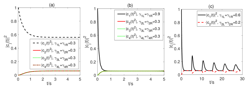
Figure 2: Evolution of four atoms coupled with a semi-infinite waveguide.

2.2 Coherent feedback control with two excitations

When initially two of the atoms are excited, and there are no photons in the waveguide, there can be overall two excitations in the quantum system. Based on Assumption 1, the quantum states in Fig. 1 (a) can be represented as

(22) $$|\Psi(t)\rangle= \sum_{1\leq j<l\leq N}c_{jl}(t)|g_{1},\cdots,e_{j},\cdots,e_{l},\cdots,g_{N},\{0\}\rangle$$

$$+\sum_{j=1}^{N}\int c_{j}^{\bullet}(t,k)|g_{1},\cdots,g_{j-1},e_{j},g_{j+1},\cdots,g_{N},\{k\}\rangle$$

$$+\int\int c_{*}(t,k_{1},k_{2})|g_{1},\cdots,g_{N},\{k_{1}\}\{k_{2}\}\rangle\mathrm{d}k_{1}\mathrm{d}k_{2},$$

where the first component represents that there are two atoms labeled with $j$ and $l$ are excited and there are no photons in the waveguide, the second component represents that the $j$th atom is excited and there is one photon of the continuous mode $k$ in the waveguide, and the last term represents that all the atoms are at their ground states and there are two photons of the mode $k_{1}$ and $k_{2}$ in the waveguide. Then the quantum state representation can be mapped on the random graph as in Definition 2.

Definition 2.

For the closed loop quantum system with feedback in Fig. 1 (b) with at most two excitations, the $j$th vertex represents that the $j$th two-level atom is excited and there is one photon in the semi-infinite waveguide; the edge between the $j$th and $l$th vertexes represents that the $j$th and $l$th two-level atoms are both excited and there are no photons in the waveguide. Then the probability of the $j$th vertex and the edge between the $j$th and $l$th vertexes reads

(23a) $$p_{j}(t)=\int|c_{j}^{\bullet}(t,k)|^{2}\mathrm{d}k,$$

(23b) $$p_{jl}(t)=|c_{jl}(t)|^{2}.$$

Take the state representation in Eq. (22) into the Schrödinger equation, then we can derive the evolution of the amplitudes as

(24a) $$\dot{c}_{jl}(t)=-i\int c_{j}^{\bullet}(t,k)g_{klt}^{*}(k,t,z_{l})\mathrm{d}k-i\int c_{l}^{\bullet}(t,k)g_{kjt}^{*}(k,t,z_{j})\mathrm{d}k,\,l\neq j,$$

(24b) $$\dot{c}_{j}^{\bullet}(t,k)=-i\sum_{l}c_{jl}(t)g_{klt}(k,t,z_{l})-i\int c_{*}(k,k_{2},t)g_{kjt}^{*}(k_{2},t,z_{j})\mathrm{d}k_{2},$$

(24c) $$\dot{c}_{*}(k_{1},k_{2},t)=-i\sum_{j}c_{j}^{\bullet}(t,k_{1})g_{kjt}(k_{2},t,z_{j})-i\sum_{j}c_{j}^{\bullet}(t,k_{2})g_{kjt}(k_{1},t,z_{j}),$$

where Eq. (24a) means that when initially one of the $N$ atoms is excited and there is one photon in the waveguide, then another atom can also be excited after absorbing the photon from the waveguide; Eq. (24b) means that when initially two atoms are excited and there are no photons in the waveguide, then one of the two excited atoms can emit one photon into the waveguide, and an atom can also absorb one photon from the waveguide if there are two photons in the waveguide; Eq. (24c) means that when there is one photon in the waveguide and one of the atoms is excited, then the excited atom can emit one photon into the waveguide to generate two-photon states.

According to the calculations in Appendix A.2, Eqs. (24a,24b) can be re-written in the delay dependent format as

$$\dot{c}_{jl}(t)=-\frac{\gamma_{jR}^{2}+\gamma_{jL}^{2}+\gamma_{lR}^{2}+\gamma_{lL}^{2}}{2}c_{jl}(t)+\gamma_{lL}\gamma_{lR}c_{jl}\left(t-\frac{2z_{l}}{c}\right)e^{i\omega_{a}\frac{2z_{l}}{c}}+\gamma_{jL}\gamma_{jR}c_{jl}\left(t-\frac{2z_{j}}{c}\right)e^{i\omega_{a}\frac{2z_{j}}{c}}$$

$$-\sum_{l^{\prime}=1,l^{\prime}>j}^{l-1}\gamma_{l^{\prime}R}\gamma_{lR}c_{jl^{\prime}}\left(t-\frac{z_{l}-z_{l^{\prime}}}{c}\right)e^{i\omega_{a}\frac{z_{l}-z_{l^{\prime}}}{c}}-\sum_{l^{\prime}=l+1,l^{\prime}>j}^{N}\gamma_{l^{\prime}L}\gamma_{lL}c_{jl^{\prime}}\left(t-\frac{z_{l^{\prime}}-z_{l}}{c}\right)e^{i\omega_{a}\frac{z_{l^{\prime}}-z_{l}}{c}}$$

$$-\sum_{j^{\prime}=1,j^{\prime}<l}^{j-1}\gamma_{j^{\prime}R}\gamma_{jR}c_{j^{\prime}l}\left(t-\frac{z_{j}-z_{j^{\prime}}}{c}\right)e^{i\omega_{a}\frac{z_{j}-z_{j^{\prime}}}{c}}-\sum_{j^{\prime}=j+1,j^{\prime}<l}^{N}\gamma_{j^{\prime}L}\gamma_{jL}c_{j^{\prime}l}\left(t-\frac{z_{j^{\prime}}-z_{j}}{c}\right)e^{i\omega_{a}\frac{z_{j^{\prime}}-z_{j}}{c}}$$

(25a) $$+\sum_{l^{\prime}\neq l}\gamma_{l^{\prime}L}\gamma_{lR}c_{jl}\left(t-\frac{z_{l}+z_{l^{\prime}}}{c}\right)e^{i\omega_{a}\frac{z_{l}+z_{l^{\prime}}}{c}}+\sum_{j^{\prime}\neq j}\gamma_{j^{\prime}L}\gamma_{jR}c_{jl}\left(t-\frac{z_{j}+z_{j^{\prime}}}{c}\right)e^{i\omega_{a}\frac{z_{j}+z_{j^{\prime}}}{c}},$$

$$\dot{c}_{j}^{\bullet}(t,k)=-\frac{\gamma_{jR}^{2}+\gamma_{jl}^{2}}{2}c_{j}^{\bullet}(t,k)-i\sum_{l}c_{jl}(t)g_{klt}(k,t,z_{l})+\sum_{j^{\prime}}\gamma_{j^{\prime}R}\gamma_{jL}c_{j}^{\bullet}\left(t-\frac{z_{j}+z_{j^{\prime}}}{c},k\right)e^{i\omega_{a}\frac{z_{j}+z_{j^{\prime}}}{c}}$$

(25b) $$-\sum_{j^{\prime}<j}\gamma_{j^{\prime}R}\gamma_{jR}c_{j}^{\bullet}\left(t-\frac{z_{j}-z_{j^{\prime}}}{c}\right)e^{i\omega_{a}\frac{z_{j}-z_{j^{\prime}}}{c}}-\sum_{j^{\prime}>j}\gamma_{j^{\prime}L}\gamma_{jL}c_{j}^{\bullet}\left(t-\frac{z_{j^{\prime}}-z_{j}}{c},k\right)e^{i\omega_{a}\frac{z_{j^{\prime}}-z_{j}}{c}},$$

where the first component of RHS of Eq. (25a) represents the spontaneous emission process of the two excited atoms into the waveguide, and the following two components represent that one atom can emit one photon into the waveuiguie and the photon can be further reflected by the terminal mirror to induce the round trip transmission delay, the second and third lines of Eq. (25a) represent the exchange of excited states between an excited atom with one of the atoms at the ground state and this process is not reflected by the mirror, and the last two components represent the exciton is transferred from one atom to another atom after the reflection by the mirror. Compared with Eq. (24b), the first part of RHS of Eq. (25b) means the spontaneous emission of the excited atom, the second part represents that one of the excited atoms can emit one photon into the waveguide, and the following three components with delays represent the transmission of excited state from one excited atom to another atom at the ground state similarly as in Eq. (25a).

Theorem 2.

[18] When $N=2$, $\gamma_{1R}=\gamma_{1L}$, $\gamma_{2R}=\gamma_{2L}$, $z_{j}=\frac{n\pi}{\omega_{a}}$ with $n=1,2,\cdots$, $c_{12}(0)=1$, then the two atoms can be continuously excited.

Then for the multi-atom network with $N>2$, we consider the special case that $z_{1}=z_{2}=\cdots=z_{N}\gg 0$, then Eq. (25) can be simplified when $t<\tau$ as

$$\dot{c}_{jl}(t)= -\frac{\gamma_{jR}^{2}+\gamma_{jL}^{2}+\gamma_{lR}^{2}+\gamma_{lL}^{2}}{2}c_{jl}(t)-\sum_{l^{\prime}=1,l^{\prime}>j}^{l-1}\gamma_{l^{\prime}R}\gamma_{lR}c_{jl^{\prime}}\left(t\right)-\sum_{l^{\prime}=l+1,l^{\prime}>j}^{N}\gamma_{l^{\prime}L}\gamma_{lL}c_{jl^{\prime}}\left(t\right)$$

(26a) $$-\sum_{j^{\prime}=1,j^{\prime}<l}^{j-1}\gamma_{j^{\prime}R}\gamma_{jR}c_{j^{\prime}l}\left(t\right)-\sum_{j^{\prime}=j+1,j^{\prime}<l}^{N}\gamma_{j^{\prime}L}\gamma_{jL}c_{j^{\prime}l}\left(t\right),$$

$$\dot{c}_{j}^{\bullet}(t,k)= -\frac{\gamma_{jR}^{2}+\gamma_{jl}^{2}}{2}c_{j}^{\bullet}(t,k)-i\sum_{l}c_{jl}(t)g_{klt}(k,t,z_{l})-\sum_{j^{\prime}<j}\gamma_{j^{\prime}R}\gamma_{jR}c_{j}^{\bullet}\left(t,k\right)$$

(26b) $$-\sum_{j^{\prime}>j}\gamma_{j^{\prime}L}\gamma_{jL}c_{j}^{\bullet}\left(t,k\right).$$

Eq. (26a) means that the amplitude representing that there are two excited atoms oscillate according to the atom-waveguide couplings. This can be interpreted with the probability of the edges of a random graph. As illustrated in Fig. 3 with $N=3$, there are three two-level atoms at $z_{j}=\frac{40\pi}{\omega_{a}}$ with $\omega_{a}=50$ and $\tau\approx 5.0265s$, initially only the first two atoms are excited as $c_{12}(0)=1$. In (a), $\gamma_{1R}=\gamma_{1L}=0.2$, $\gamma_{2R}=\gamma_{2L}=\gamma_{3R}=\gamma_{3L}=1$, then when $t<\tau$, both the first and the second atom can emit coherent fields into the waveguide, and that can be absorbed by the third atom, then the first and the third, or the second and the third atoms can be simultaneously excited. Specially in (b), $\gamma_{1R}=\gamma_{1L}=\gamma_{2R}=\gamma_{2L}=0.2$, $\gamma_{3R}=\gamma_{3L}=1$, $c_{13}$ and $c_{23}$ evolve with the same parameter settings according to Eq. (26a) and can reach population consensus.

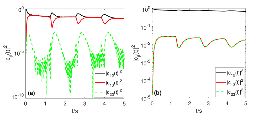
Figure 3: Consensus evolution of four atoms with two excitations coupled with a semi-infinite waveguide.

Above all, in this section we have analyzed the coherent feedback dynamics based on the quantum network that multiple two-level atoms are coupled with a semi-infinite waveguide. In the following, we analyze how the coherent feedback dynamcis will be influenced by the environment in the open quantum systems.

3 Hybrid coherent and measurement feedback control

In practical quantum systems, the quantum dynamics is influenced by the environment. For example, an initially excited atom in Fig. 1(a) cannot be perfectly coupled with the waveguide, and can spontaneously decay to the environment. Thus the conclusions in Section 2 cannot perfectly hold because of the influence by the environment. To eliminate the influence of the environment, external drives must be applied on the atoms to generate the desired quantum states. Take the case that only one atom at $z_{1}$ with the resonant frequency $\omega_{a1}$ is coupled with the semi-infinite waveguide, so that the Hamiltonian of the system with a coherent drive on the atom reads [21]

(27) $$H_{t}= \left(\omega_{a1}-i\gamma_{0}\right)\sigma_{1}^{+}\sigma_{1}^{-}+\frac{1}{2}\left(\Omega_{1}\sigma_{1}^{-}+\Omega_{1}^{*}\sigma_{1}^{+}\right)+\int_{0}^{\infty}\mathrm{d}k\omega_{k}d^{{\dagger}}_{k}d_{k}$$

$$+\int\mathrm{d}k[g_{k1t}(k,t,z_{1})d^{{\dagger}}_{k}\sigma_{1}^{-}+g_{k1t}^{*}(k,t,z_{1})d_{k}\sigma_{1}^{+}],$$

where $\gamma_{0}$ is the atom’s spontaneous decaying rate to the environment, $\Omega_{1}=\bar{\Omega}_{1}e^{i\bar{\omega}_{1}t}$ represents a coherent drive with the Rabi frequency $\bar{\Omega}_{1}$ at a frequency $\bar{\omega}_{1}$, and we denote the detuning between the coherent drive and the atom as $\delta_{1}=\bar{\omega}_{1}-\omega_{a1}$ [21, 15]. Then we denote the atomic Hamiltonian in a rotating frame as [21, 15]

(28) $$H_{s}=-\left(\delta_{1}+i\gamma_{0}\right)\sigma_{1}^{+}\sigma_{1}^{-}+\frac{1}{2}\left(\bar{\Omega}_{1}\sigma_{1}^{-}+H.C.\right).$$

For simplification, in the following we first take $\gamma_{0}=0$ to derive the quantum control dynamics and then analyze how $\gamma_{0}$ will influence the performance. Take the atom as concerned system, and the waveguide as an environment, then we can write the master equation as [46, 47, 48, 49]

(29) $$\dot{\rho}(t)=-i\left[H_{\mathrm{eff}},\rho(t)\right]+\Gamma_{\mathrm{eff}}\left(\sigma_{1}^{-}\rho(t)\sigma_{1}^{+}-\frac{1}{2}\rho(t)\sigma_{1}^{+}\sigma_{1}^{-}-\frac{1}{2}\sigma_{1}^{+}\sigma_{1}^{-}\rho(t)\right),$$

where

$$H_{\mathrm{eff}}=-\delta_{1}\sigma_{1}^{+}\sigma_{1}^{-}+\frac{1}{2}\left(\bar{\Omega}_{1}\sigma_{1}^{-}+H.C.\right)-\gamma_{1L}\gamma_{1R}\sin\left(\omega_{a}\frac{2z_{1}}{c}\right)\sigma_{1}^{+}\sigma_{1}^{-},$$

$\Gamma_{\mathrm{eff}}=y_{\gamma}+\Gamma$, $y_{\gamma}=\frac{\gamma_{1R}^{2}+\gamma_{1L}^{2}}{2}-\gamma_{1L}\gamma_{1R}\cos\left(\omega_{a}\frac{2z_{1}}{c}\right)$. $y_{\gamma}$ represents the dissipation rate from the atom to the waveguide, and $\Gamma\geq 0$ represents the dissipation of the waveguide mode to the environment, which can be induced by the practical imperfect design such as that the atom is not at the central of the waveguide as in Ref. [50]. Above all, $\Gamma_{\mathrm{eff}}\geq 0$ where the equation holds only when $\Gamma=0$, $\gamma_{1R}=\gamma_{1L}$ and $\cos\left(\omega_{a}\frac{2z_{1}}{c}\right)=1$.

Remark 3.1.

When initially the atom is excited, $\delta_{1}=\bar{\Omega}_{1}=\Gamma=0$, $\gamma_{1R}=\gamma_{1L}$ and $\omega_{a}\frac{2z_{1}}{c}=2n\pi$ with $n=1,2,\cdots$, then $\dot{\rho}(t)=0$, then the atom is continuously excited, as introduced in Refs. [51, 18, 52, 53, 16, 54].

Denote $X=\sigma_{1}^{-}+\sigma_{1}^{+}$, and $Y=\delta_{1}+\gamma_{1L}\gamma_{1R}\sin\left(\omega_{a}\frac{2z_{1}}{c}\right)$. Then we can derive the evolution of the following operators as

(30a) $$\frac{\mathrm{d}}{\mathrm{d}t}\langle X\rangle=iY\left(\langle\sigma_{1}^{-}\rangle-\langle\sigma_{1}^{+}\rangle\right)-\frac{\Gamma_{\mathrm{eff}}}{2}\left(\langle\sigma_{1}^{-}\rangle+\langle\sigma_{1}^{+}\rangle\right),$$

(30b) $$\frac{\mathrm{d}}{\mathrm{d}t}\langle\sigma_{1}^{+}\rangle=-iY\langle\sigma_{1}^{+}\rangle-\frac{\Gamma_{\mathrm{eff}}}{2}\langle\sigma_{1}^{+}\rangle-\frac{i\bar{\Omega}}{2}\langle\sigma_{1}^{z}\rangle,$$

(30c) $$\frac{\mathrm{d}}{\mathrm{d}t}\langle\sigma_{1}^{-}\rangle=iY\langle\sigma_{1}^{-}\rangle-\frac{\Gamma_{\mathrm{eff}}}{2}\langle\sigma_{1}^{-}\rangle+\frac{i\bar{\Omega}}{2}\langle\sigma_{1}^{z}\rangle,$$

(30d) $$\frac{\mathrm{d}}{\mathrm{d}t}\langle\sigma_{1}^{z}\rangle=-i\bar{\Omega}\left(\langle\sigma_{1}^{+}\rangle-\langle\sigma_{1}^{-}\rangle\right)-\Gamma_{\mathrm{eff}}\left(\langle\sigma_{1}^{z}\rangle+1\right).$$

Denote $\tilde{X}=\left[\langle\sigma_{1}^{+}\rangle,\langle\sigma_{1}^{-}\rangle,\langle\sigma_{1}^{z}\rangle\right]^{\mathrm{T}}$ with $\mathrm{T}$ for the transpose matrix, then

(31) $$\dot{\tilde{X}} =\begin{bmatrix}-iY-\frac{\Gamma_{\mathrm{eff}}}{2}&0&-\frac{i\bar{\Omega}}{2}\\ 0&iY-\frac{\Gamma_{\mathrm{eff}}}{2}&\frac{i\bar{\Omega}}{2}\\ -i\bar{\Omega}&i\bar{\Omega}&-\Gamma_{\mathrm{eff}}\end{bmatrix}\tilde{X}-\begin{bmatrix}0\\ 0\\ \Gamma_{\mathrm{eff}}\end{bmatrix}$$

$$\triangleq A\tilde{X}-B,$$

and

(32) $$\langle X\rangle =\begin{bmatrix}1&1&0\end{bmatrix}\tilde{X} \triangleq C\tilde{X}.$$

Denote $\tilde{\textbf{X}}(s)$ as the Laplace transformation of $\tilde{X}$, $\textbf{X}(s)$ as that of $\langle X\rangle$, then we have

(33) $$s\tilde{\textbf{X}}(s)-\tilde{X}(0)=A\tilde{\textbf{X}}(s)-\frac{1}{s}B,$$

(34) $$\tilde{\textbf{X}}(s)=\left(sI-A\right)^{-1}\left(\tilde{X}(0)-\frac{1}{s}B\right),$$

and

(35) $$\textbf{X}(s)=C\left(sI-A\right)^{-1}\left(\tilde{X}(0)-\frac{1}{s}B\right).$$

Then

(36) $$|sI-A| =\left(\left(s+\frac{\Gamma_{\mathrm{eff}}}{2}\right)^{2}+Y^{2}\right)\left(s+\Gamma_{\mathrm{eff}}\right)+\bar{\Omega}^{2}\left(s+\frac{\Gamma_{\mathrm{eff}}}{2}\right).$$

Denote $Z(s)$ as the Laplace transformation of $\langle\sigma_{1}^{z}\rangle$, which is determined by the initial condition of the system. We analyze the atomic dynamics according to the following assumption.

Assumption 2.

Assume initially $\tilde{X}(0)=\left[0,0,z_{0}\right]^{\mathrm{T}}$ with $-1\leq z_{0}\leq 1$.

Then

(37) $$Z(s) =\frac{\left(z_{0}-\frac{\Gamma_{\mathrm{eff}}}{s}\right)\left[\left(s+\frac{\Gamma_{\mathrm{eff}}}{2}\right)^{2}+Y^{2}\right]}{\left(\left(s+\frac{\Gamma_{\mathrm{eff}}}{2}\right)^{2}+Y^{2}\right)\left(s+\Gamma_{\mathrm{eff}}\right)+\bar{\Omega}^{2}\left(s+\frac{\Gamma_{\mathrm{eff}}}{2}\right)}.$$

Theorem 3.

In the open quantum system with $\Gamma>0$, the atomic state is determined by the coherent drive, chiral couplings between the atom and waveguide, and the initial state of the atom, then the steady value of $\langle\sigma_{1}^{z}\rangle=-\frac{\Gamma_{\mathrm{eff}}^{2}+4Y^{2}}{\Gamma_{\mathrm{eff}}^{2}+4Y^{2}+2\bar{\Omega}^{2}}<0$ always holds when $\Gamma_{\mathrm{eff}}\neq 0$.

Proof.

According to Eq. (37), the steady value of $\langle\sigma_{1}^{z}\rangle$ reads

(38) $$\langle\sigma_{1}^{z}(\infty)\rangle =\lim_{s\rightarrow 0}\frac{s\left(z_{0}-\frac{\Gamma_{\mathrm{eff}}}{s}\right)\left[\left(s+\frac{\Gamma_{\mathrm{eff}}}{2}\right)^{2}+Y^{2}\right]}{\left(\left(s+\frac{\Gamma_{\mathrm{eff}}}{2}\right)^{2}+Y^{2}\right)\left(s+\Gamma_{\mathrm{eff}}\right)+\bar{\Omega}^{2}\left(s+\frac{\Gamma_{\mathrm{eff}}}{2}\right)}$$

$$=-\frac{\Gamma_{\mathrm{eff}}^{2}+4Y^{2}}{\Gamma_{\mathrm{eff}}^{2}+4Y^{2}+2\bar{\Omega}^{2}}<0,$$

where the second equation holds when $\Gamma_{\mathrm{eff}}\neq 0$.

Theorem 4.

[31] Consider the quantum control system Hamiltonian $H_{0}$, operator $L$ in the Lindblad component, and $\left[H_{0},L\right]\neq 0$, then there is at least one eigenstate of $H_{0}$ denoted as $\rho_{d}$, such that the trace distance between the quantum state $\rho(t)$ and $\rho_{d}$ valued by $D\left(\rho(t),\rho_{d}\right)$ satisfies that

$$\limsup_{t\rightarrow\infty}D\left(\rho(t),\rho_{d}\right)>0.$$

Remark 3.2.

Theorem 4 means that when the dissipation operator does not commute with the atomic operator, there is at least one eigenstate which cannot be prepared with arbitrary high fidelity no matter how the external control is designed. In our case with coherent and measurement feedback based on waveguide QED, $L=\sigma_{1}^{-}$ does not commute with the atomic Hamiltonian, the atom cannot be continuously excited when the waveguide dissipates to the environment with the rate $\Gamma>0$ in Eq. (29). This agrees with the conclusion in Ref. [50] that $\Gamma$ can provide a new dissipation channel to prevent the atom’s excitation.

3.1 An example when $\gamma_{0}\neq 0$ and $\Gamma=0$

When $\gamma_{0}\neq 0$ and $\Gamma=0$, denote $Y^{\prime}=Y+i\gamma_{0}$ and $\Gamma_{\mathrm{eff}}^{\prime}=y_{\gamma}$, the initial atomic state is given as Assumption 2, then the steady state of the atom can be modified according to Eq. (37) as

(39) $$Z^{\prime}(s) =\frac{\left(z_{0}-\frac{\Gamma_{\mathrm{eff}}^{\prime}}{s}\right)\left[\left(s+\frac{\Gamma_{\mathrm{eff}}^{\prime}}{2}\right)^{2}+Y^{\prime 2}\right]}{\left(\left(s+\frac{\Gamma_{\mathrm{eff}}^{\prime}}{2}\right)^{2}+Y^{\prime 2}\right)\left(s+\Gamma_{\mathrm{eff}}^{\prime}\right)+\bar{\Omega}^{2}\left(s+\frac{\Gamma_{\mathrm{eff}}^{\prime}}{2}\right)}.$$

Theorem 5.

When $Y=0$, the atom can be continuously excited and the population of excited stated is determined by the coherent drive and decaying to the environment.

Proof.

When $Y=0$, $Y^{\prime}=i\gamma_{0}$, then

(40) $$\langle\sigma_{1}^{z}(\infty)\rangle =\frac{s\left(z_{0}-\frac{\Gamma_{\mathrm{eff}}^{\prime}}{s}\right)\left[\left(s+\frac{\Gamma_{\mathrm{eff}}^{\prime}}{2}\right)^{2}+Y^{\prime 2}\right]}{\left(\left(s+\frac{\Gamma_{\mathrm{eff}}^{\prime}}{2}\right)^{2}+Y^{\prime 2}\right)\left(s+\Gamma_{\mathrm{eff}}^{\prime}\right)+\bar{\Omega}^{2}\left(s+\frac{\Gamma_{\mathrm{eff}}^{\prime}}{2}\right)}$$

$$=\frac{4\gamma_{0}^{2}-\Gamma_{\mathrm{eff}}^{\prime 2}}{2\bar{\Omega}^{2}-4\gamma_{0}^{2}+\Gamma_{\mathrm{eff}}^{\prime 2}}.$$

Remark 3.3.

When $\bar{\Omega}^{2}=4\gamma_{0}^{2}-\Gamma_{\mathrm{eff}}^{\prime 2}$, $\langle\sigma_{1}^{z}(\infty)\rangle=1$, this means that the coherent drive can compensate the atom’s spontaneous decaying process to the environment and the atom can be ideally excited.

3.2 Measurement feedback control combined with the coherent feedback

When the quantum system is measured via the Homodyne detection at the right end of the semi-infinite waveguide with the measurement operator $\sigma_{1}^{-}$, then the dynamics can be represented as [55]

(41) $$\mathrm{d}\rho(t) =-i[H_{\mathrm{eff}},\rho(t)]\mathrm{d}t+\Gamma_{\mathrm{eff}}\mathcal{L}_{\sigma_{1}^{-}}\left[\rho(t)\right]\mathrm{d}t+\mathcal{H}[\gamma_{1R}\sigma_{1}^{-}]\rho(t)\sqrt{\eta}dW,$$

$\mathcal{L}_{\sigma_{1}^{-}}$ is the Lindblad component in Eq. (29), $dW$ is a Wiener process with $E(dW)=0$ and $E\left[dW^{2}\right]=\mathrm{d}t$, $\eta$ is homodyne detection efficiency, we neglect the induced phase by the local oscillator and for an arbitrary operator $L$,

$$\mathcal{H}[L]\rho=L\rho(t)+\rho(t)L^{{\dagger}}-Tr\left[\right(L+L^{{\dagger}}\left)\rho(t)\right]\rho(t).$$

The homodyne detection result reads

(42) $$I_{c}(t) =\gamma_{1R}\langle X\rangle+\frac{1}{\sqrt{\eta\gamma}}\frac{dW}{\mathrm{d}t}$$

$$\triangleq\gamma_{1R}\langle X\rangle+\frac{1}{\sqrt{\eta\gamma}}\xi(t),$$

where $0<\gamma\leq 1$ represents the measurement strength. In the following, we assume $\eta=\gamma=1$. Then the measurement feedback control equation with the operator $F$ reads [56, 22, 57, 1]

(43) $$\mathrm{d}\rho(t)=-i[H_{\mathrm{eff}},\rho(t)]\mathrm{d}t+\Gamma_{\mathrm{eff}}\mathcal{L}_{\sigma_{1}^{-}}\left[\rho(t)\right]\mathrm{d}t+\mathcal{H}[\gamma_{1R}\sigma_{1}^{-}]\rho(t)\mathrm{d}W(t)$$

$$-ig_{f}\left[F,\rho(t)\right]\mathrm{d}W(t)-ig_{f}\gamma_{1R}\left[F,\sigma_{1}^{-}\rho(t)+\rho(t)\sigma_{1}^{+}\right]\mathrm{d}t-\frac{1}{2}g_{f}^{2}\left[F,\left[F,\rho(t)\right]\right]\mathrm{d}t,$$

where $g_{f}$ represents the feedback strength.

When $H_{\mathrm{eff}}=-\left(Y+i\gamma_{0}\right)\sigma_{1}^{+}\sigma_{1}^{-}+\frac{1}{2}\bar{\Omega}_{1}X$, $F=X$ [36], the evolution of the operators reads

(44a) $$\frac{\mathrm{d}}{\mathrm{d}t}\langle X\rangle=i\left(Y+i\gamma_{0}\right)\left(\langle\sigma_{1}^{-}\rangle-\langle\sigma_{1}^{+}\rangle\right)-\frac{\Gamma_{\mathrm{eff}}}{2}\left(\langle\sigma_{1}^{-}\rangle+\langle\sigma_{1}^{+}\rangle\right)+\gamma_{1R}\left(1+\langle\sigma_{1}^{z}\rangle-\langle X\rangle^{2}\right)\xi(t),$$

$$\frac{\mathrm{d}}{\mathrm{d}t}\langle\sigma_{1}^{+}\rangle=-i\left(Y+i\gamma_{0}\right)\langle\sigma_{1}^{+}\rangle-\frac{\Gamma_{\mathrm{eff}}}{2}\langle\sigma_{1}^{+}\rangle-\frac{i\bar{\Omega}}{2}\langle\sigma_{1}^{z}\rangle+ig_{f}\gamma_{1R}\langle X\rangle+g_{f}^{2}\left(\langle\sigma_{1}^{-}\rangle-\langle\sigma_{1}^{+}\rangle\right)$$

(44b) $$~{}~{}~{}~{}~{}~{}~{}~{}~{}~{}~{}~{}~{}+\gamma_{1R}\left(\frac{1+\langle\sigma_{1}^{z}\rangle}{2}-\langle X\rangle\langle\sigma_{1}^{+}\rangle\right)\xi(t)-ig_{f}\langle\sigma_{1}^{z}\rangle\xi(t),$$

$$\frac{\mathrm{d}}{\mathrm{d}t}\langle\sigma_{1}^{-}\rangle=i\left(Y+i\gamma_{0}\right)\langle\sigma_{1}^{-}\rangle-\frac{\Gamma_{\mathrm{eff}}}{2}\langle\sigma_{1}^{-}\rangle+\frac{i\bar{\Omega}}{2}\langle\sigma_{1}^{z}\rangle-ig_{f}\gamma_{1R}\langle X\rangle+g_{f}^{2}\left(\langle\sigma_{1}^{+}\rangle-\langle\sigma_{1}^{-}\rangle\right)$$

(44c) $$~{}~{}~{}~{}~{}~{}~{}~{}~{}~{}~{}~{}~{}+\gamma_{1R}\left(\frac{1+\langle\sigma_{1}^{z}\rangle}{2}-\langle X\rangle\langle\sigma_{1}^{-}\rangle\right)\xi(t)+ig_{f}\langle\sigma_{1}^{z}\rangle\xi(t),$$

$$\frac{\mathrm{d}}{\mathrm{d}t}\langle\sigma_{1}^{z}\rangle=-i\bar{\Omega}\left(\langle\sigma_{1}^{+}\rangle-\langle\sigma_{1}^{-}\rangle\right)-\Gamma_{\mathrm{eff}}\left(\langle\sigma_{1}^{z}\rangle+1\right)-2g_{f}^{2}\langle\sigma_{1}^{z}\rangle$$

(44d) $$~{}~{}~{}~{}~{}~{}~{}~{}~{}~{}~{}~{}~{}-\gamma_{1R}\langle X\rangle\left(1+\langle\sigma_{1}^{z}\rangle\right)\xi(t)-2ig_{f}\left(\langle\sigma_{1}^{+}\rangle-\langle\sigma_{1}^{-}\rangle\right)\xi(t).$$

Take $\xi(t)=0$, and compare with Eq. (30), we can derive that

(45) $$\mathcal{A} =\begin{bmatrix}-i\left(Y-g_{f}\gamma_{1R}\right)+\gamma_{0}-\frac{\Gamma_{\mathrm{eff}}}{2}-g_{f}^{2}&g_{f}^{2}&-\frac{i\bar{\Omega}}{2}\\ g_{f}^{2}&i\left(Y-g_{f}\gamma_{1R}\right)-\gamma_{0}-\frac{\Gamma_{\mathrm{eff}}}{2}-g_{f}^{2}&\frac{i\bar{\Omega}}{2}\\ -i\bar{\Omega}&i\bar{\Omega}&-\Gamma_{\mathrm{eff}}-2g_{f}^{2}\end{bmatrix},$$

and the Laplace transformation of $\langle\sigma_{1}^{z}\rangle$ reads

(46) $$\mathcal{Z}(s)=\frac{z_{0}-\Gamma_{\mathrm{eff}}/s}{\left(s+\Gamma_{\mathrm{eff}}+2g_{f}^{2}\right)+\frac{2g_{f}^{2}\bar{\Omega}^{2}+\bar{\Omega}^{2}\left(s+\Gamma_{\mathrm{eff}}/2\right)}{\left(s+\Gamma_{\mathrm{eff}}/2+g_{f}^{2}\right)^{2}-\left[i\left(Y-g_{f}\gamma_{1R}\right)-\gamma_{0}\right]^{2}-g_{f}^{4}}}.$$

Theorem 6.

The measurement feedback control cannot drive the atom to be fully excited but can enhance its convergence to the state with $\langle\sigma_{1}^{z}\rangle=0$, which can be evaluated by the feedback strength $g_{f}^{2}$ when $Y,\gamma_{0}\ll g_{f}\gamma_{1R}$.

Proof.

By Theorem 4 and Remark 3.2, the atom cannot be continuously excited. We consider the steady value

(47) $$\langle\sigma_{1}^{z}(\infty)\rangle =\lim_{s\rightarrow 0}s\mathcal{Z}(s)$$

$$=\frac{-\Gamma_{\mathrm{eff}}}{\left(\Gamma_{\mathrm{eff}}+2g_{f}^{2}\right)+\frac{\bar{\Omega}^{2}\left(2g_{f}^{2}+\frac{\Gamma_{\mathrm{eff}}}{2}\right)}{\frac{\Gamma_{\mathrm{eff}}}{2}\left(2g_{f}^{2}+\frac{\Gamma_{\mathrm{eff}}}{2}\right)-\left[i\left(Y-g_{f}\gamma_{1R}\right)-\gamma_{0}\right]^{2}}}<0.$$

When $Y,\gamma_{0}\ll g_{f}\gamma_{1R}$,

(48) $$\langle\sigma_{1}^{z}(\infty)\rangle \approx\frac{-\Gamma_{\mathrm{eff}}}{\left(\Gamma_{\mathrm{eff}}+2g_{f}^{2}\right)+\frac{\bar{\Omega}^{2}\left(2g_{f}^{2}+\frac{\Gamma_{\mathrm{eff}}}{2}\right)}{\frac{\Gamma_{\mathrm{eff}}}{2}\left(2g_{f}^{2}+\frac{\Gamma_{\mathrm{eff}}}{2}\right)+g_{f}^{2}\gamma_{1R}^{2}}}$$

$$=\frac{-\Gamma_{\mathrm{eff}}}{\left(\Gamma_{\mathrm{eff}}+2g_{f}^{2}\right)+\frac{2\bar{\Omega}^{2}}{\Gamma_{\mathrm{eff}}+\frac{4g_{f}^{2}\gamma_{1R}^{2}}{4g_{f}^{2}+\Gamma_{\mathrm{eff}}}}},$$

where $g_{f}$ can enhance the convergence of $\langle\sigma_{1}^{z}(\infty)\rangle$ to zero.

Remark 3.4.

For a special case that $\bar{\Omega}=0$, which means that the atom is only driven by the measurement feedback control field, then $\langle\sigma_{1}^{z}(\infty)\rangle=-\frac{\Gamma_{\mathrm{eff}}}{\Gamma_{\mathrm{eff}}+2g_{f}^{2}}$.

Based on Remark 3.4, we can derive the following theorem on how the homodyne detection noise can influence the amplitudes of quantum state around its final steady state. These results are derived without considering measurement noises.

Theorem 7.

When $g_{f}\gg\gamma_{1R}$, the stochastic component in the amplitude of atom is smallest when the atom is nonchirally coupled with the waveguide, compared with the chiral circumstance. For the given coupling, the stochastic component in the amplitude is the smallest when $z_{1}$ approaches $\frac{n\pi c}{\omega_{a}}$ and the largest when $z_{1}$ approaches $\frac{(2n+1)\pi c}{2\omega_{a}}$ with $n=0,1,2,\cdots$.

Proof.

When $\xi(t)\neq 0$, we denote $\langle\sigma_{1}^{+}\rangle=\bar{\langle\sigma_{1}^{+}\rangle}+\Delta\sigma_{1}^{+}$, $\langle\sigma_{1}^{-}\rangle=\bar{\langle\sigma_{1}^{-}\rangle}+\Delta\sigma_{1}^{-}$, $\langle\sigma_{1}^{z}\rangle=\bar{\langle\sigma_{1}^{z}\rangle}+\Delta\sigma_{1}^{z}$, where $\bar{\langle\sigma_{1}^{+}\rangle}$, $\bar{\langle\sigma_{1}^{-}\rangle}$ and $\bar{\langle\sigma_{1}^{z}\rangle}$ represent the mean value of the operators in Eq. (44) with $\bar{\Omega}=0$ and $\xi(t)=0$, $\Delta\sigma_{1}^{+}$, $\Delta\sigma_{1}^{z}$ and $\Delta\sigma_{1}^{z}$ are the stochastic values induced by $\xi(t)\neq 0$. Similar as Eq. (48), we can derive that $\bar{\langle\sigma_{1}^{+}\rangle}=\bar{\langle\sigma_{1}^{-}\rangle}=\bar{\langle\sigma_{1}^{z}\rangle}=0$. When $g_{f}\gg\Gamma_{\mathrm{eff}}$, the dominant stochastic component in Eq. (44d) is proportional to

(49) $$\langle\sigma_{1}^{+}\rangle-\langle\sigma_{1}^{-}\rangle =\Delta\sigma_{1}^{+}-\Delta\sigma_{1}^{-}=-2ig_{f}\langle\sigma_{1}^{z}\rangle dW$$

$$=-2ig_{f}\left(\bar{\langle\sigma_{1}^{z}\rangle}+\Delta\sigma_{1}^{z}\right)dW$$

$$=-2ig_{f}\bar{\langle\sigma_{1}^{z}\rangle}dW$$

$$=2ig_{f}\frac{\Gamma_{\mathrm{eff}}}{\Gamma_{\mathrm{eff}}+2g_{f}^{2}}dW,$$

where $\Delta\sigma_{1}^{z}dW$ is omitted because $\mathrm{d}W^{2+n}=0$ for $n>0$ [58]. According to Eq. (48) with $\bar{\Omega}=0$, the final steady value is determined by $V=\frac{g_{f}^{2}}{\Gamma_{\mathrm{eff}}}$, then for given $V$ with $g_{f}\gg\Gamma_{\mathrm{eff}}$,

(50) $$\langle\sigma_{1}^{+}\rangle-\langle\sigma_{1}^{-}\rangle =2ig_{f}\frac{\Gamma_{\mathrm{eff}}}{\Gamma_{\mathrm{eff}}+2g_{f}^{2}}dW$$

$$=2i\frac{\sqrt{V\Gamma_{\mathrm{eff}}}}{1+2V}dW.$$

This means that the settings $\gamma_{1L}=\gamma_{1R}$ or $z_{1}=\frac{n\pi c}{\omega_{a}}$ in Theorem 7 with smaller $\Gamma_{\mathrm{eff}}$ can induce better stability of the quantum state around its steady value.

Theorem 8.

When $\omega_{a}z_{1}=n\pi$ with $n=1,2,\cdots$ and $g_{f}\gg\gamma_{1R}$ does not hold, chiral couplings between the atom and waveguide can induce faster atomic transient evolutions.

Proof.

Consider the dynamics in Eq. (44d) with $\xi(t)=0$ and $\bar{\Omega}=0$. When $\omega_{a}z_{1}=n\pi$, $\Gamma_{\mathrm{eff}}$ will be real positive. When the atom converges to the same steady state with given $V$, then $g_{f}=\sqrt{\Gamma_{\mathrm{eff}}V}$. For $\gamma_{1R}$ and $\gamma_{1L}$ with the same sum, $\Gamma_{\mathrm{eff}}$ and $g_{f}$ will be larger when $\gamma_{1R}\neq\gamma_{1L}$. Then $\langle\sigma_{1}^{z}\rangle$ approaches to its steady value with faster convergence.

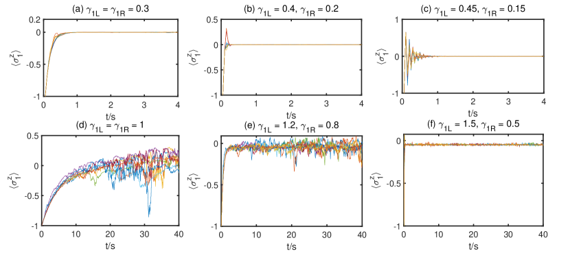
Figure 4: Measurement feedback control influenced by coherent feedback designs.

As illustrated in Fig. 4(a-c), $\omega_{a}=50$, $\gamma_{0}=0$, $\bar{\Omega}=0$, $\Gamma=0.01$, $\mathrm{d}t=0.05s$, initially the atom is at the ground state and finally converges to the same steady value by making sure that $\frac{g_{f}^{2}}{\Gamma_{\mathrm{eff}}}=300$. When $z_{1}=\frac{\pi}{\omega_{a}}$, the chiral couplings between the atom and the waveguide can induce larger $\Gamma_{\mathrm{eff}}$, ($\Gamma_{\mathrm{eff}}=0.01,0.03,0.055$ in (a-c), respectively), then the influence of the quantum state amplitudes can be larger. This agrees with the conclusion in Theorem 7. In Fig. 4(d-f), the parameters are the same as (a-c) except the coupling strengths and $\frac{g_{f}^{2}}{\Gamma_{\mathrm{eff}}}=10$. Then in (d) $\Gamma_{\mathrm{eff}}=0.01$, in (e) $\Gamma_{\mathrm{eff}}=0.09$ and in (f) $\Gamma_{\mathrm{eff}}=0.51$. Then $\langle\sigma_{1}^{z}\rangle$ converges faster with larger $\Gamma_{\mathrm{eff}}$ and this agrees with the conclusion in Theorem 8.

4 Conclusions

We have studied the feedback control based on the architecture that two-level atoms are coupled to a semi-infinite waveguide. In the closed quantum system, when initially there are no more than two atoms that are excited and the waveguide is empty, the quantum system evolution can be interpreted as the evolution of a random graph. By adjusting the location of the atoms and the chiral coupling strengths between the atom and the waveguide, the number of photons and the consensus of the atoms can be contolled. In the open quantum system, the spontaneous emission and dissipation of the atom induced by the environment can influence the final steady quantum state, while this process can be compensated by the external drives and measurement feedback controls. Simultaneously, the coherent feedback can be tuned by designing the chiral couplings and the location of the atom, and this can influence the oscillation of atomic states driven by the measurement feedback control with homodyne detection noises.

Appendix A Derivation of the delay dependent control equation with one and two excitations based on the Schrödinger equation

In this section, we derive the delay dependent control equation in the main text according to the number of possible excitations emitted by the atoms in the waveguide. Section A.1 introduces the details on the derivation of Eq. (6) with one excitation and section A.2 introduces that for Eq. (25) with two excitations.

A.1 Derivation of Eq. (6)

The integration of Eq. (5b) into Eq. (5a) gives

(51) $$~{}~{}~{}~{}\dot{c}_{j}(t)=-i\int g_{kjt}^{*}(k,t,z_{j})\tilde{c}(t,k)\mathrm{d}k$$

$$=\int\left[-\gamma_{jR}e^{-i\left[\left(\omega_{k}-\omega_{a}\right)t-\omega z_{j}/c\right]}+\gamma_{jL}e^{-i\left[\left(\omega_{k}-\omega_{a}\right)t+\omega z_{j}/c\right]}\right]$$

$$~{}~{}~{}~{}\left[\sum_{p=1}^{N}\int_{0}^{t}c_{p}(u)\left[\gamma_{pR}e^{i\left[\left(\omega_{k}-\omega_{a}\right)u-\omega z_{p}/c\right]}-\gamma_{pL}e^{i\left[\left(\omega_{k}-\omega_{a}\right)u+\omega_{k}z_{p}/c\right]}\right]\mathrm{d}u\right]\mathrm{d}k$$

$$=-\frac{\gamma_{jR}^{2}+\gamma_{jL}^{2}}{2}c_{j}(t)-\gamma_{jR}\sum_{p=1}^{j-1}\gamma_{pR}c_{p}\left(t-\frac{z_{j}-z_{p}}{c}\right)e^{i\omega_{a}\frac{z_{j}-z_{p}}{c}}$$

$$~{}~{}~{}~{}+\gamma_{jR}\sum_{p=1}^{N}\gamma_{pL}c_{p}\left(t-\frac{z_{p}+z_{j}}{c}\right)e^{i\omega_{a}\frac{z_{p}+z_{j}}{c}}$$

$$~{}~{}~{}~{}-\gamma_{jL}\sum_{p=j+1}^{N}\gamma_{pL}c_{p}\left(t-\frac{z_{p}-z_{j}}{c}\right)e^{i\omega_{a}\frac{z_{p}-z_{j}}{c}}.$$

Now we take one of the integrations in the second and third line of Eq. (51) as an example, we have

(52) $$~{}~{}~{}~{}\gamma_{jR}\int_{0}^{t}c_{p}(u)\int\gamma_{pR}e^{i\left[\left(\omega_{k}-\omega_{a}\right)u-\omega_{k}z_{p}/c\right]}e^{-i\left[\left(\omega_{k}-\omega_{a}\right)t-\omega_{k}z_{j}/c\right]}\mathrm{d}k\mathrm{d}u$$

$$=\gamma_{jR}\int_{0}^{t}c_{p}(u)\gamma_{pR}e^{i\omega_{a}(t-u)}\delta\left(u-t-z_{p}/c+z_{j}/c\right)\mathrm{d}u$$

$$=\gamma_{jR}\gamma_{pR}c_{p}\left(t-\frac{z_{j}-z_{p}}{c}\right)e^{i\omega_{a}\frac{z_{j}-z_{p}}{c}}.$$

The other components in Eq. (6) can be derived similarly.

A.2 Derivation of the delay dependent control equation with two excitations

Take Eq. (24c) into Eq. (24b), the second component of the RHS of Eq. (24b) reads

(53) $$~{}~{}~{}~{}i\int c_{*}(k,k_{2},t)g_{kjt}^{*}(k_{2},t,z_{j})\mathrm{d}k_{2}$$

$$=\int\int_{0}^{t}\sum_{j^{\prime}}\left[c_{j^{\prime}}^{\bullet}(u,k)g_{kj^{\prime}t}(k_{2},u,z_{j})+c_{j^{\prime}}^{\bullet}(u,k_{2})g_{kj^{\prime}t}(k,u,z_{j^{\prime}})\right]\mathrm{d}ug_{kjt}^{*}(k_{2},t,z_{j})\mathrm{d}k_{2}$$

$$=\sum_{j^{\prime}}\int\int_{0}^{t}\left[c_{j^{\prime}}^{\bullet}(u,k)g_{kj^{\prime}t}(k_{2},u,z_{j^{\prime}})+c_{j^{\prime}}^{\bullet}(u,k_{2})g_{kj^{\prime}t}(k,u,z_{j^{\prime}})\right]g_{kjt}^{*}(k_{2},t,z_{j})\mathrm{d}u\mathrm{d}k_{2}$$

$$=\sum_{j^{\prime}}\int_{0}^{t}\int c_{j^{\prime}}^{\bullet}(u,k)\left(\gamma_{j^{\prime}R}e^{-ik_{2}z_{j^{\prime}}}-\gamma_{j^{\prime}L}e^{ik_{2}z_{j^{\prime}}}\right)$$

$$~{}~{}~{}~{}\left(\gamma_{jR}e^{ik_{2}z_{j}}-\gamma_{jL}e^{-ik_{2}z_{j}}\right)e^{ik_{2}c(u-t)}\mathrm{d}k_{2}e^{i\omega_{a}(t-u)}\mathrm{d}u$$

$$=\sum_{j^{\prime}}\int_{0}^{t}c_{j^{\prime}}^{\bullet}(u,k)\left[\gamma_{j^{\prime}R}\gamma_{jR}\delta\left(u-t+\frac{z_{j}-z_{j^{\prime}}}{c}\right)-\gamma_{j^{\prime}R}\gamma_{jL}\delta\left(u-t-\frac{z_{j}+z_{j^{\prime}}}{c}\right)\right.$$

$$~{}~{}~{}~{}\left.-\gamma_{j^{\prime}L}\gamma_{jR}\delta\left(u-t+\frac{z_{j}+z_{j^{\prime}}}{c}\right)+\gamma_{j^{\prime}L}\gamma_{jL}\delta\left(u-t+\frac{z_{j^{\prime}}-z_{j}}{c}\right)\right]e^{i\omega_{a}(t-u)}\mathrm{d}u$$

$$=\frac{\gamma_{jR}^{2}+\gamma_{jl}^{2}}{2}c_{j}^{\bullet}(t,k)-\sum_{j^{\prime}}\gamma_{j^{\prime}R}\gamma_{jL}c_{j}^{\bullet}\left(t-\frac{z_{j}+z_{j^{\prime}}}{c},k\right)e^{i\omega_{a}\frac{z_{j}+z_{j^{\prime}}}{c}}$$

$$~{}~{}~{}~{}+\sum_{j^{\prime}<j}\gamma_{j^{\prime}R}\gamma_{jR}c_{j}^{\bullet}\left(t-\frac{z_{j}-z_{j^{\prime}}}{c}\right)e^{i\omega_{a}\frac{z_{j}-z_{j^{\prime}}}{c}}$$

$$~{}~{}~{}~{}+\sum_{j^{\prime}>j}\gamma_{j^{\prime}L}\gamma_{jL}c_{j}^{\bullet}\left(t-\frac{z_{j^{\prime}}-z_{j}}{c},k\right)e^{i\omega_{a}\frac{z_{j^{\prime}}-z_{j}}{c}},$$

which is the delay dependent evolution format in Eq. (25b).

Then for the right part of Eq. (24a),

(54) $$~{}~{}~{}~{}\int c_{j}^{\bullet}(t,k)g_{klt}^{*}(k,t,z_{l})\mathrm{d}k$$

$$=\sum_{l^{\prime}}\int_{0}^{t}\int-ic_{jl^{\prime}}(u)g_{kl^{\prime}t}(k,u,z_{l^{\prime}})g_{klt}^{*}(k,t,z_{l})\mathrm{d}k\mathrm{d}u$$

$$=-i\sum_{l^{\prime}}\int_{0}^{t}\int c_{jl^{\prime}}(u)\left[\gamma_{l^{\prime}R}\gamma_{lR}e^{i\omega_{k}\left(u-t+\frac{z_{l}-z_{l^{\prime}}}{c}\right)}-\gamma_{l^{\prime}R}\gamma_{lL}e^{i\omega_{k}\left(u-t-\frac{z_{l}+z_{l^{\prime}}}{c}\right)}\right.$$

$$~{}~{}~{}~{}\left.-\gamma_{l^{\prime}L}\gamma_{lR}e^{i\omega_{k}\left(u-t+\frac{z_{l}+z_{l^{\prime}}}{c}\right)}+\gamma_{l^{\prime}L}\gamma_{lL}e^{i\omega_{k}\left(u-t+\frac{z_{l^{\prime}}-z_{l}}{c}\right)}\right]e^{i\omega_{a}(t-u)}\mathrm{d}k\mathrm{d}u$$

$$=-i\sum_{l^{\prime}=1}^{l-1}\int_{0}^{t}\gamma_{l^{\prime}R}\gamma_{lR}c_{jl^{\prime}}(u)\delta\left(u-t+\frac{z_{l}-z_{l^{\prime}}}{c}\right)e^{i\omega_{a}(t-u)}\mathrm{d}u$$

$$~{}~{}~{}~{}+i\sum_{l^{\prime}=1}^{l-1}\int_{0}^{t}c_{jl^{\prime}}(u)\gamma_{l^{\prime}L}\gamma_{lR}\delta\left(u-t+\frac{z_{l}+z_{l^{\prime}}}{c}\right)e^{i\omega_{a}(t-u)}\mathrm{d}u$$

$$~{}~{}~{}~{}-i\sum_{l^{\prime}=l+1}^{N}\int_{0}^{t}\gamma_{l^{\prime}L}\gamma_{lL}c_{jl^{\prime}}(u)\delta\left(u-t+\frac{z_{l^{\prime}}-z_{l}}{c}\right)e^{i\omega_{a}(t-u)}\mathrm{d}u-i\frac{\gamma_{lR}^{2}+\gamma_{lL}^{2}}{2}c_{jl}(t)$$

$$=-i\sum_{l^{\prime}=1,l^{\prime}\neq j}^{l-1}\gamma_{l^{\prime}R}\gamma_{lR}c_{jl^{\prime}}\left(t-\frac{z_{l}-z_{l^{\prime}}}{c}\right)e^{i\omega_{a}\frac{z_{l}-z_{l^{\prime}}}{c}}$$

$$~{}~{}~{}~{}+i\sum_{l^{\prime}=1,l^{\prime}\neq j}^{N}\gamma_{l^{\prime}L}\gamma_{lR}c_{jl^{\prime}}\left(t-\frac{z_{l}+z_{l^{\prime}}}{c}\right)e^{i\omega_{a}\frac{z_{l}+z_{l^{\prime}}}{c}}$$

$$~{}~{}~{}~{}-i\sum_{l^{\prime}=l+1,l^{\prime}\neq j}^{N}\gamma_{l^{\prime}L}\gamma_{lL}c_{jl^{\prime}}\left(t-\frac{z_{l^{\prime}}-z_{l}}{c}\right)e^{i\omega_{a}\frac{z_{l^{\prime}}-z_{l}}{c}}\mathrm{d}u-i\frac{\gamma_{lR}^{2}+\gamma_{lL}^{2}}{2}c_{jl}(t),$$

which is half of the components in Eq. (25a) and the other half can be similarly derived.