Forster–Warmuth Counterfactual Regression: A Unified Learning Approach

Abstract

Series or orthogonal basis regression is one of the most popular non-parametric regression techniques in practice, obtained by regressing the response on features generated by evaluating the basis functions at observed covariate values. The most routinely used series estimator is based on ordinary least squares fitting, which is known to be minimax rate optimal in various settings, albeit under fairly stringent restrictions on the basis functions and the distribution of covariates. In this work, inspired by the recently developed Forster-Warmuth (FW) learner (Forster and Warmuth, 2002), we propose an alternative series regression estimator that can attain the minimax estimation rate under strictly weaker conditions imposed on the basis functions and the joint law of covariates, than existing series estimators in the literature. Moreover, a key contribution of this work generalizes the FW-learner to a so-called counterfactual regression problem, in which the response variable of interest may not be directly observed (hence, the name “counterfactual”) on all sampled units, and therefore needs to be inferred in order to identify and estimate the regression in view from the observed data. Although counterfactual regression is not entirely a new area of inquiry, we propose the first-ever systematic study of this challenging problem from a unified pseudo-outcome perspective. In fact, we provide what appears to be the first generic and constructive approach for generating the pseudo-outcome (to substitute for the unobserved response) which leads to the estimation of the counterfactual regression curve of interest with small bias, namely bias of second order. Several applications are used to illustrate the resulting FW-learner including many nonparametric regression problems in missing data and causal inference literature, for which we establish high-level conditions for minimax rate optimality of the proposed FW-learner.

Abstract

This supplement contains the proofs of all the main results in the paper and some supporting lemmas.

1 Introduction

1.1 Nonparametric regression

Nonparametric estimation plays a central role in many statistical contexts where one wishes to learn conditional distributions by means of say, a conditional mean function $\mathbb{E}[Y|X=x]$ without a priori restriction on the model. Several other functionals of the conditional distribution can likewise be written based on conditional means, which makes the conditional mean an important problem to study. For example, the conditional cumulative distribution function of a univariate response $Y$ given $X=x$ can be written as $\mathbb{E}[\mathbf{1}\{Y\leq t\}|X=x].$ This, in turn, leads to conditional quantiles. In general, any conditional function defined via $\theta^{\star}(x)=\operatorname*{arg\,min}_{\theta\in\mathbb{R}}\mathbb{E}[\rho((X,Y);\theta)|X=x]$ for any loss function $\rho(\cdot;\cdot)$ can be learned using conditional means.

Series, or more broadly, sieve estimation provides a solution by approximating an unknown function based on $k$ basis functions, where $k$ may grow with the sample size $n$, ideally at a rate carefully tuned in order to balance bias and variance to the extent possible. The most straightforward approach to construct a series estimator is by the method of least squares, large sample properties of which have been studied extensively both in statistical and econometrics literature in nonparametric settings. To briefly describe the standard least squares series estimator, let $m^{\star}(x):=\mathbb{E}[Y|X=x]$ denote the true conditional expectation where $m^{\star}(\cdot)$ is an unrestricted unknown function of $x$. Also consider a vector of approximating basis functions $\widebar{\phi}_{k}(x)=(\phi_{1}(x),\ldots,\phi_{k}(x))^{\top}$, which has the property that any square integrable $m^{\star}(\cdot)$ can be approximated arbitrarily well, with sufficiently large $k$, by some linear combination of $\widebar{\phi}_{k}(\cdot)$. Let $(X_{i},Y_{i}),i=1,\dots,n$ denote an observed sample of data. The least squares series estimator of $m^{\star}(x)$ is defined as $\widehat{m}(x)=\bar{\phi}_{k}^{\top}(x)\widehat{\beta}$, where $\widehat{\beta}=(\Phi_{k}^{\top}\Phi_{k})^{-1}\Phi_{k}^{\top}\mathbf{Y}$, and $\Phi_{k}$ is the $n\times k$ matrix $[\widebar{\phi}_{k}(X_{1}),\dots,\widebar{\phi}_{k}(X_{n})]^{\top}$ with $\mathbf{Y}=(Y_{1},\dots,Y_{n})^{\top}$. Several existing works in the literature provide sufficient conditions for consistency, corresponding convergence rates, and asymptotic normality of this estimator, along with illustrations of these conditions in the case of polynomial series and regression splines, see, for example, Chen (2007), Newey (1997), Györfi et al. (2002). Under these conditions, the optimal rate of convergence are well-established for certain bases functions, such as the local polynomial kernel estimator (Chapter 1.6 of Tsybakov (2009)) and the local polynomial partition series (Cattaneo and Farrell (2013)). Belloni et al. (2015) relaxed some of these assumptions while applying this estimation procedure to statistical estimation problems and provided uniform convergence rates. For instance, they weakened the requirement in Newey (1997) that the number $k$ of approximating functions has to satisfy $k^{2}/n\rightarrow 0$ to $k/n\rightarrow 0$ for bounded (for example Fourier series) or local bases (such as splines, wavelets or local polynomial partition series), which was previously established only for splines (Huang (2003)) and local polynomial partitioning estimators (Cattaneo and Farrell (2013)); therefore presumably allowing for improved approximation of the function in view by using a larger number of basis functions to estimate the latter. One important limitation of least squares series estimator is that the rate of convergence heavily depends on stringent assumptions imposed on the bases functions. To be specific, a key quantity that plays a crucial role in all of these previous works, is given by $\xi_{k}:=\sup_{x\in\mathcal{X}}\|\phi_{k}(x)\|$, where $\mathcal{X}$ is the support of the covariates $X$ and $\|\cdot\|$ denote the $l_{2}$ norm of a vector. They require $\xi_{k}^{2}\log k/n\rightarrow 0$, so that for bases functions such as Fourier, splines, wavelets, and local polynomial partition series, $\xi_{k}\leq\sqrt{k}$, yielding $k\log k/n\rightarrow 0$. For other bases functions such as polynomial series, $\xi_{k}\lesssim k$ corresponds to $k^{2}\log k/n\rightarrow 0$, which is more restrictive.

In this paper, we develop a new type of series regression estimator that in principle can attain well-established minimax nonparametric rates of estimation in settings where covariates and outcomes are fully observed, under weaker conditions compared to existing literature (e.g. Belloni et al. (2015)) on the distribution of covariates and bases functions. The approach builds on an estimator we refer to as Forster–Warmuth Learner (FW-Learner) originating in the online learning literature, which is obtained via a careful modification of the renowned non-linear Vovk–Azoury–Warmuth forecaster (Vovk, 2001; Forster and Warmuth, 2002). In particular, our method is optimal in that its error matches the well-established minimax rate of estimation for a large class of smooth nonparametric regression functions, provided that $\mathbb{E}[Y^{2}|X]$ is bounded almost surely, regardless of the basis functions used, as long as the approximation error/bias with $k$ bases decays optimally; see Theorem 1 for more details. This result is more general than the current literature whose rate of convergence depends on the type of basis. For example, Belloni et al. (2015) established that using the polynomials basis would imply a slower convergence rate compared to using a wavelet basis, although both have the same approximation error decay rate for the common Hölder/Sobolev spaces. Theorem 1 provides the expected $L_{2}$-error of our FW-Learner under the full data setting, which is a non-trivial extension of the vanilla Forster–Warmuth estimator and is agnostic to the underlying choice of bases functions. The sharp upper bound on the error rate matches the minimax lower bound of this problem, demonstrating the optimality of the FW-Learner.

1.2 Counterfactual regression

Moving beyond the traditional conditional mean estimation problem, we also develop a unified approach to study a more challenging class of problems we name nonparametric counterfactual regression, where the goal is still to estimate $m^{\star}(x)=\mathbb{E}[Y|X=x]$ but now the response $Y$ may not be fully/directly observed.

Prominent examples include nonparameric regression of an outcome prone to missingness, a canonical problem in missing data literature, as well as nonparametric estimation of the so-called conditional average treatment effect (CATE) central to causal inference literature. Thus, the key contribution of this work, is to deliver a unified treatment of such counterfactual regression problems with a generic estimation approach which essentially consists of two steps: (i) generate for all units a carefully constructed pseudo-outcome of the counterfactual outcome of interest; (ii) apply the FW-Learner directly to the counterfactual pseudo-outcome, in order to obtain an estimator of the counterfactual regression in view. The counterfactual pseudo-outcome in step (i) is motivated by modern semiparametric efficiency theory and may be viewed as an element of the orthogonal complement of the nuisance tangent space for the statistical model of the given counterfactual regression problem, see, e.g., Bickel et al. (1993), Van Der Vaart (1991), Newey (1990), Tsiatis (2006) for some references; as such the pseudo-outcome endows the FW-Learner with a “small bias” property that its bias is at most of a second order. In some key settings, the bias of the pseudo-outcome might be sufficiently small, occasionally it might even be exactly zero, so that it might altogether be ignored without an additional condition. This is in fact the case if the outcome were a priori known to be missing completely at random, such as in some two-stage sampling problems where missingness is by design, e.g. (Breslow and Cain, 1988); or if estimating the CATE in a randomized experiment where the treatment mechanism is known by design. More generally, the pseudo-outcome often requires estimating certain nuisance functions nonparametrically, however, for a large class of such problems considered in this paper, the bias incurred from such estimation is of product form, also known as mixed bias (Rotnitzky et al. (2021)). In this context, a key advantage of the mixed bias is that one’s ability to estimate one of the nuisance functions well, i.e. relatively “fast rates”, can potentially make up for slower rates in estimating another, so that, estimation bias of the pseudo-outcome can be negligible relative to the estimation risk of an oracle with ex ante knowledge of nuisance functions. In such cases, the FW-Learner is said to be oracle optimal in the sense that its risk matches that of the oracle (up to a multiplicative constant).

Our main theoretical contribution is a unified analysis of the FW-Learner described above, hereby establishing that it attains the oracle optimality property, under appropriate regularity conditions, in several important counterfactual regression problems, including (1) nonparametric regression under outcome missing at random, (2) nonparametric CATE estimation under unconfoundedness, (3) nonparametric regression under outcome missing not at random leveraging a so-called shadow variable (Li et al., 2021; Miao et al., 2023), (4) nonparametric CATE estimation in the presence of residual confounding leveraging proxies using the proximal causal inference framework (Miao et al., 2018; Tchetgen Tchetgen et al., 2020).

1.3 Literature review, organization, and notation

Organization.

The remainder of the paper is organized as follows. Section 1.4 introduces the notation that is going to be used throughout the paper. Section 2 formally defines our estimation problem and the Forster–Warmuth estimator, where Section 2.2 builds upon Section 2.1 going beyond the full data problem to counterfactual settings where the outcome of interest may not be fully observed. Section 3 applies the proposed methods to the canonical nonparametric regression problem subject to missing outcome data, where in Section 3.1 the outcome is assumed to be Missing At Random (MAR) given fully observed covariates Robins et al. (1994); while in Section 3.2 the outcome may be Missing Not At Random (MNAR) and identification hinges upon having access to a fully observed shadow variable (Miao et al., 2023; Li et al., 2021). Both of these examples may be viewed as nonparametric counterfactual regression models, whereby one seeks to estimate the nonparametric regression function under a hypothetical intervention that would in principle prevent missing data. Section 4 presents another application of the proposed methods to a causal inference setting, where the nonparametric counterfactual regression parameter of interest is the Conditional Average Treatment Effect (CATE); Section 4.1 assumes the so-called ignorability or unconfoundedness given fully observed covariates, while Section 4.2 accommodates unmeasured confounding for which proxy variables are observed under the recently proposed proximal causal inference framework (Miao et al., 2018; Tchetgen Tchetgen et al., 2020). Section 5 reports results from a simulation study comparing our proposed FW-Learner to a selective set of existing methods under a range of conditions, while Section 6 illustrates FW-Learner for the CATE in an analysis of the SUPPORT observational study (Conners et al. (1996)) to estimate the causal effect of right heart catheterization (RHC) on 30-day survival, as a function of a continuous baseline covariate which measures a patient’s potential survival probability at hospital admission, both under standard unconfoundedness conditions assumed in prior causal inference papers, including Tan (2006), Vermeulen and Vansteelandt (2015) and Cui and Tchetgen Tchetgen (2019), and proximal causal inference conditions recently considered in Cui et al. (2023) in the context of estimating marginal treatment effects.

Literature Review.

There is growing interest in nonparametric/semiparametric regression problems involving high dimensional nuisance functions. Notable general frameworks recently proposed to address rich classes of such problems include Ai and Chen (2003) and Foster and Syrgkanis (2019), with the latter providing an oracle inequality for empirical risk minimization under the condition that an estimated loss function uniquely characterizing a nonparametric regression function of interest satisfies a form of orthogonality property, more precisely, that the estimated loss function admits second order bias. In another strand of work related to nonparametric regression with missing data on the outcome, Müller and Schick (2017) investigated the efficiency of a complete-case nonparametric regression under an outcome missing at random assumption (MAR); relatedly, Efromovich (2011) proposed a nonparametric series estimator that is shown to be minimax when predictors are missing completely at random (MCAR), and Wang et al. (2010) proposed an augmented inverse probability weighted nonparametric regression kernel estimator using parametric specifications of nuisance functions in the setting of an outcome missing at random. In the context of CATE estimation for causal inference, in a setting closely related to ours, Kennedy (2020) proposed a doubly robust two-stage CATE estimator, called the DR-Learner, and provided a general oracle inequality for nonparametric regression with estimated outcomes. In the same paper, he also proposed a local polynomial adaptation of the R-Learner (Nie and Wager (2021), Robinson (1988)), and characterized its (in-probability) point-wise error rate. He referred to this new estimator as Local Polynomial R-Learner (lp-R-Learner). Notably, the lp-R-Learner was shown to attain the corresponding oracle rate under weaker smoothness conditions for nuisance functions and the CATE than analogous estimators in Nie and Wager (2021) and Chernozhukov et al. (2017). The recent work of Kennedy et al. (2022) studied the minimax lower bound for the rate of estimation of the CATE under unconfoundedness (in terms of mean squared error) and proposed higher order estimators using recent estimation theory of higher-order influence functions (Robins et al., 2008, 2017) that is minimax optimal provided the covariate distribution is sufficiently smooth that it can be estimated at fast enough rates so that estimation bias is negligible. Another related strand of work has focused on so-called meta-Learners based on generic machine learning estimators. For instance, Künzel et al. (2019) proposed two learners (X-Learner and U-Learner) for CATE estimation through generic machine learning. In Section 5, we provide a simulation study comparing our proposed method to the X-Learner, the DR-Learner and to an oracle DR-Learner which uses the Oracle pseudo-outcome with known nuisance functions in the second-stage regression.

In Section 4 we apply our method to estimating CATE, the average effect of the treatment for individuals who have specific values of a set of baseline covariates. By inferring CATE, researchers can potentially identify subgroups of the population that may benefit most from the treatment; information that is crucial for designing effective interventions tailored to the individual. Similar to Kennedy (2020) and Kennedy et al. (2022), we study this problem under the unconfoundedness assumption in Section 4.1. While their proposed lp-learner, which leverages the careful use of local polynomials to estimate the CATE, was shown to match an oracle estimator with complete knowledge of all nuisance parameters under certain smoothness conditions, our proposed FW-Learner is shown to match the oracle estimator for more general bases functions under minimal conditions on the latter. Therefore, in this light, our estimator affords the analyst with the freedom to use an arbitrary bases functions of choice to model the CATE.

In many non-experimental practical settings, un-confoundedness may not be credible on the basis of measured covariates, in which case, one may be concerned that residual confounding due to hidden factors may bias inferences about the CATE using the above methods. To address such concerns, the recent so-called “proximal causal inference” approach acknowledges that measured covariates are unlikely to fully control for confounding and may at best be viewed as proxies of known but unmeasured sources of confounding, see, e.g., Miao et al. (2018) and Tchetgen Tchetgen et al. (2020), where they formally leverage proxies for nonparametric identification of causal effects in the presence of hidden confounders. In Section 4.2, we develop an FW-proximal learner of the CATE using the proposed pseudo-outcome approach in which we leverage a characterization of the ortho-complement to the nuisance tangent space for the underlying proximal causal model derived in Cui et al. (2023), also see Ghassami et al. (2022). It is worth mentioning that recent concurrent work Sverdrup and Cui (2023) also estimates CATE under the proximal causal inference context with what they call a P-Learner using a two-stage loss function approach inspired by the R-Learner proposed in Nie and Wager (2021), which, in order to be oracle optimal, requires that the nuisance functions are estimated at rates faster than $n^{-1/4}$, a requirement we do not impose.

1.4 Notation

We define some notation we use throughout the paper: $a\lesssim b$ means $a\leq Cb$ for a universal constant $C$, and $a\sim b$ means $a\lesssim b$ and $b\lesssim a$. We call a function $\alpha$-smooth if it belongs to the class of Hölder smoothness order $\alpha$, which will be introduced using similar language as Belloni et al. (2015): For $\alpha\in(0,1]$, the Hölder class of smoothness order $\alpha,\Sigma_{\alpha}(\mathcal{X})$, is defined as the set of all functions $f:\mathcal{X}\rightarrow\mathbb{R}$ such that for $C>0$,

$$|f(x)-f(\widetilde{x})|\leq C\Bigl{(}\sum_{j=1}^{d}\bigl{(}x_{j}-\widetilde{x}_{j}\bigr{)}^{2}\Bigr{)}^{\alpha/2}$$

for all $x=\left(x_{1},\ldots,x_{d}\right)^{\top}$ and $\widetilde{x}=\left(\widetilde{x}_{1},\ldots,\widetilde{x}_{d}\right)^{\top}$ in $\mathcal{X}$. The smallest $C$ satisfying this inequality defines a norm of $f$ in $\Sigma_{\alpha}(\mathcal{X})$, which we denote by $\|f\|_{s(\alpha)}.$ For $\alpha>1,\Sigma_{\alpha}(\mathcal{X})$ can be defined as follows. For a $d$-tuple $\bar{\alpha}=\left(\alpha_{1},\ldots,\alpha_{d}\right)$ of non-negative integers, let $D^{\bar{\alpha}}=\partial_{x_{1}}^{\alpha_{1}}\ldots\partial_{x_{d}}^{\alpha_{d}}$ be the multivariate partial derivative operator. Let $\lfloor\alpha\rfloor$ denote the largest integer strictly smaller than $\alpha$. Then $\Sigma_{\alpha}(\mathcal{X})$ is defined as the set of all functions $f:\mathcal{X}\rightarrow\mathbb{R}$ such that $f$ is $\lfloor\alpha\rfloor$ times continuously differentiable and for some $C>0$,

$$\bigl{|}D^{\bar{\alpha}}f(x)-D^{\bar{\alpha}}f(\widetilde{x})\bigr{|}\leq C\Bigl{(}\sum_{j=1}^{d}\bigl{(}x_{j}-\widetilde{x}_{j}\bigr{)}^{2}\Bigr{)}^{(\alpha-\lfloor\alpha\rfloor)/2}\text{ and }\bigl{|}D^{\bar{\beta}}f(x)\bigr{|}\leq C$$

for all $x=\left(x_{1},\ldots,x_{d}\right)^{\prime}$ and $\widetilde{x}=\left(\widetilde{x}_{1},\ldots,\widetilde{x}_{d}\right)^{\prime}$ in $\mathcal{X}$ and for all $d$-tuples $\bar{\alpha}=\left(\alpha_{1},\ldots,\alpha_{d}\right)$ and $\bar{\beta}=\left(\beta_{1},\ldots,\beta_{d}\right)$ of non-negative integers satisfying $\alpha_{1}+\cdots+\alpha_{d}=\lfloor\alpha\rfloor$ and $\beta_{1}+\cdots+\beta_{d}\leq\lfloor\alpha\rfloor.$ Again, the smallest $C$ satisfying these inequalities defines a norm of $f$ in $\Sigma_{\alpha}(\mathcal{X})$, denoted as $\|f\|_{s(\alpha)}$. For any integer $k\geq 2$, let $\|f(\cdot)\|_{k}$ denote the function $L_{k}$ norm such that $\|f(O)\|_{k}:=(\mathbb{E}_{O}[f^{k}(O)])^{1/k},$ where $O$ is any data that is the input of $f$.

2 The Forster–Warmuth Nonparametric Counterfactual Regression Estimator

We introduce the Forster–Warmuth learner, which is a nonparametric extension of an estimator first proposed in the online learning literature (Forster and Warmuth, 2002). In Section 2.1, we study the properties of FW-Learner in the standard nonparametric regression setting where data are fully observed, before considering the counterfactual setting of primary interest in Section 2.2 where the responses may only be partially observed.

2.1 Full data nonparametric regression

Suppose that one observes independent and identically distributed observations $\left(X_{i},Y_{i}\right),1\leq i\leq n$ on $\mathcal{X}\times\mathbb{R}$. Let $\mu$ be a base measure on the covariate space $\mathcal{X}$; this could, for example, be the Lebesgue measure or the countable measure. The most common nonparametric regression problem aims to infer the conditional mean function $m^{\star}(x):=\mathbb{E}\left[Y_{i}\mid X_{i}=x\right]$ as a function of $x$. Let $\Psi:=\left\{\phi_{1}(\cdot)\equiv 1,\phi_{2}(\cdot),\phi_{3}(\cdot),\ldots\right\}$ be a fundamental sequence of functions in $L_{2}(\mu)$ i.e., linear combinations of these functions are dense in $L_{2}(\mu)$ (Lorentz, 1966; Yang and Barron, 1999). Note that a fundamental sequence of functions need not be orthonormal.

For any $f\in L_{2}(\mu)$ and any $J\geq 1$, let

$$E_{J}^{\Psi}(f)~{}:=~{}\min_{a_{1},a_{2},\ldots,a_{J}}\left\|f-\sum_{k=1}^{J}a_{k}\phi_{k}\right\|_{L_{2}(\mu)}$$

denote the $J$-th degree approximation error of the function $f$ by the first $J$ functions in $\Psi$. By definition of the fundamental sequence, $E_{J}^{\Psi}(f)\to 0$ as $J\to 0$ for any function $f\in L_{2}(\mu)$. This fact is the motivation of the traditional series estimators of $m^{\star}$ which estimate the minimizing coefficients $a_{1},\ldots,a_{J}$ using ordinary least squares linear regression. Motivated by an estimator in the linear regression setting studied in Forster and Warmuth (2002), we define the FW-Learner of $m^{\star}(\cdot)$, which we denote $\widehat{m}_{J}(\cdot)$, trained on data $\{\left(X_{i},Y_{i}\right),1\leq i\leq n\},$ using the first $J$ elements of the fundamental sequence $\bar{\phi}_{J}(x)=\bigl{(}\phi_{1}(x),\ldots,\phi_{J}(x)\bigr{)}^{\top}$:

$$\widehat{m}_{J}(x):=\bigl{(}1-h_{n}(x)\bigr{)}\bar{\phi}_{J}^{\top}(x)\Bigl{(}\sum_{i=1}^{n}\bar{\phi}_{J}(X_{i})\bar{\phi}_{J}^{\top}(X_{i})+\bar{\phi}_{J}(x)\bar{\phi}_{J}^{\top}(x)\Bigr{)}^{-1}\sum_{i=1}^{n}\bar{\phi}_{J}(X_{i})Y_{i},$$ (1)

where

$$h_{n}(x):=\bar{\phi}_{J}^{\top}(x)\Bigl{(}\sum_{i=1}^{n}\bar{\phi}_{J}(X_{i})\bar{\phi}^{\top}_{J}(X_{i})+\bar{\phi}_{J}(x)\bar{\phi}^{\top}_{J}(x)\Bigr{)}^{-1}\bar{\phi}_{J}(x)~{}\in~{}[0,1].$$ (2)

The following result provides a finite-sample result on the estimation error of $\widehat{m}_{J}$ as a function of $J$.

Theorem 1.

Suppose $\mathbb{E}\bigl{[}Y^{2}|X\bigr{]}\leq\sigma^{2}$ almost surely $X$ and suppose $X$ has a density with respect to $\mu$ that is upper bounded by $\kappa$. Then the FW-Learner satisfies

$$\bigl{\|}\widehat{m}_{J}-m^{\star}\bigr{\|}_{2}^{2}=\mathbb{E}\Bigl{[}\bigl{(}\widehat{m}_{J}(X)-m^{\star}(X)\bigr{)}^{2}\Bigr{]} ~{}\leq~{}\frac{2\sigma^{2}J}{n}+\kappa(E_{J}^{\Psi}(m^{*}))^{2}.$$

Moreover, if $\Gamma=\{\gamma_{1},\gamma_{2},\ldots\}$ is a non-increasing sequence and if $m^{\star}\in\mathcal{F}(\Psi,\Gamma)=\{f\in L_{2}(\mu):\,\mathbb{E}_{k}^{\Psi}(f)\leq\gamma_{k}\,\forall\,k\geq 1\}$, then for $J_{n}:=\min\{k\geq 1:\,\gamma_{k}^{2}\leq\sigma^{2}k/n\}$, we obtain

$$\|\widehat{m}_{J_{n}}-m^{\star}\|_{2}^{2}~{}\leq~{}(2+\kappa)\frac{\sigma^{2}J_{n}}{n}.$$

See Section S.2 of the supplement for proof of this result. Note that Belloni et al. (2015, Theorem 4.1) established a similar result for the least squares series estimator implying that it yields the same oracle risk under more stringent conditions imposed on the bases functions as discussed in the introduction. The sets of functions $\mathcal{F}(\Psi,\Gamma)$ are called full approximation sets in Lorentz (1966) and Yang and Barron (1999, Section 4). If the sequence $\Gamma$ also satisfies the condition $0<c^{\prime}\leq\gamma_{2k}/\gamma_{k}\leq c\leq 1$ for all $k\geq 1$, then Theorem 7 of Yang and Barron (1999) proves that the minimax rate of estimation of functions in $\mathcal{F}(\Psi,\Gamma)$ is given by $k_{n}/n$, where $k_{n}$ is chosen so that $\gamma_{k}^{2}\asymp k/n$. The upper bound in Theorem 1 matches this rate under the assumption $c^{\prime}\leq\gamma_{2k}/\gamma_{k}\leq c$. This can be proved as follows: by definition of $J_{n}$, $\gamma_{J_{n}-1}^{2}\geq\sigma^{2}(J_{n}-1)/n$. Then using $J_{n}-1\geq J_{n}/2$ and $\gamma_{J_{n}-1}\leq\gamma_{J_{n}/2}\leq\gamma_{J_{n}}/c^{\prime}$, we get $\gamma_{J_{n}}^{2}\geq(c^{\prime})^{2}\sigma^{2}J_{n}/(2n)$. Hence, $\gamma_{J_{n}}\asymp\sigma^{2}J_{n}/n$. Therefore, Theorem 1 proves that the FW-Learner with a properly chosen $J$ is minimax optimal for approximation sets.

Note that Theorem 1 does not require the fundamental sequence of functions $\Psi$ to form an orthonormal bases. This is a useful feature when considering sieve-based estimators (Shen and Wong, 1994, Example 3), or partition-based estimators (Cattaneo and Farrell, 2013) or random kitchen sinks (Rahimi and Recht, 2008) or neural networks (Klusowski and Barron, 2018), just to name a few.

As a special case of Theorem 1 that is of particular interest for Hölder or Sobolev spaces, suppose $\gamma_{J}\leq C_{m}J^{-2\alpha_{m}/d}$ for some constant $C_{m},\alpha_{m}>0$, and $d$ is the intrinsic dimension of the covariates $X$, then choosing $J=\lceil\left(n\alpha_{m}\kappa C_{m}/(d\sigma^{2})\right)^{d/(2\alpha_{m}+d)}\rceil$ gives

$$\|\widehat{m}_{J}-m^{\star}\|_{2}^{2} \leq C\left(\frac{\sigma^{2}}{n}\right)^{2\alpha_{m}/(2\alpha_{m}+d)},$$ (3)

where $C$ is a constant; See S.2 for a proof. The decay condition $\gamma_{J}\leq C_{m}J^{-2\alpha_{m}/d}$ is satisfied by functions in Hölder and Sobolev spaces for the classical polynomial, Fourier/trigonometric bases (DeVore and Lorentz, 1993; Belloni et al., 2015)

From the discussion above, it is clear that the choice of the number of functions $J$ used is crucial for attaining the minimax rate. In practice, we propose the use of split-sample cross-validation to determine $J$ (Györfi et al., 2002, Section 7.1). Our simulations presented in Section 5 shows good performance of such an approach. We refer interested readers to Györfi et al. (2002, Chapter 7) and Vaart et al. (2006) for the theoretical properties of the split-sample cross-validation. The application of these results to FW-Learner is beyond the scope of the current paper and will be explored elsewhere.

2.2 Forster–Warmuth Counterfactual Regression: The Pseudo-Outcome Approach

In many practical applications in health and social sciences it is not unusual for an outcome to be missing on some subjects, either by design, say in two-stage sampling studies where the outcome can safely be assumed to be missing at random with known non-response mechanism, or by happenstance, in which case the outcome might be missing not at random. An example of the former type might be a study (Cornelis et al., 2009) in which one aims to develop a polygenic risk prediction model for type-2 diabetes based on stage 1 fully observed covariate data on participants including high dimensional genotype (i.e., SNPs), age, and gender, while costly manual chart review by a panel of physicians yield reliable type-2 diabetes labels on a subset of subjects with known selection probability based on stage-1 covariates. In contrast, an example of the latter type might be a household survey in Zambia (Marden et al., 2018) in which eligible household members are asked to test for HIV, however, nearly $30\%$ decline the test and thus have missing HIV status. The concern here might be that participants who decline to test might not be a priori exchangeable with participants who agree to test for HIV with respect to key risk factors for HIV infection, even after adjusting for fully observed individual and household characteristics collected in the household survey. Any effort to build an HIV risk regression model that generalizes to the wider population of Zambia requires carefully accounting for HIV status possibly missing not at random for a non-negligible fraction of the sample.

Beyond missing data, counterfactual regression also arises in causal inference where one might be interested in the CATE, the average causal effect experienced by a subset of the population defined in terms of observed covariates. Missing data, in this case, arises as the causal effect defined at the individual level as a difference between two potential outcomes – one for each treatment value – can never be observed. This is because under the consistency assumption (Hernán and Robins, 2010, Section 3.4) the observed outcome for subjects who actually received treatment matches their potential outcome under treatment, while their potential outcome under no treatment is missing, and vice-versa for the untreated.

A major contribution of this paper is to propose a generic construction of a so-called pseudo-outcome which, as its name suggests, replaces the unobserved outcome with a carefully constructed response variable that (i) only depends on the observed data, possibly involving high dimensional nuisance functions that can nonetheless be identified from the observed data (e.g. propensity score), and therefore can be evaluated for all subjects in the sample and; (ii) has conditional expectation given covariates that matches the counterfactual regression of interest if as for an oracle, nuisance functions were known. The proposed pseudo-outcome approach applies to a large class of counterfactual regression problems including the missing data and causal inference problems described above. The proposed approach recovers in specific cases such as the CATE under unconfoundedness, previously proposed forms of pseudo-outcomes (Kennedy, 2020, Section 4.2), while offering new pseudo-outcome constructions in other examples (e.g., Proximal CATE estimation in Section 4.2). See Section 2.3 for details on constructing pseudo-outcomes.

Before describing the explicit construction of the pseudo-outcome, we first provide a key high-level corollary (assuming that a pseudo-outcome is given) which is the theoretical backbone of our approach. Suppose $\widetilde{O}_{i},1\leq i\leq n$ represents independent and identically distributed random vectors of unobserved data of primary interest that include fully observed covariates $X_{i},1\leq i\leq n$ as subvectors. Let $O_{i},1\leq i\leq n$ be the observed data which are obtained from $\widetilde{O}_{i},1\leq i\leq n$ through some coarsening operation. For concrete examples of $\widetilde{O}_{i}$ and $O_{i}$ in missing data and causal inference, see Table 1; more examples can be found in Sections 3 and 4. The quantity of interest is $m^{\star}(x)=\mathbb{E}[\widetilde{f}(\widetilde{O}_{i})|X_{i}=x]$ for some known function $\widetilde{f}(\cdot)$ operating on $\widetilde{O}_{i}$. For example, in the context of missing data, we could be interested in $\mathbb{E}[Y_{i}|X_{i}]$ so that $\widetilde{f}(\widetilde{O}_{i})=f(X_{i},Z_{i},Y_{i})=Y_{i}$. Because $\widetilde{O}_{i},1\leq i\leq n$ are unobserved, $\widetilde{f}(\widetilde{O}_{i})$ may not be fully observed. The pseudo-outcome approach that we propose involves two steps:

1. Find some identifying conditions such that that quantity of interest $m^{\star}(x)=\mathbb{E}[\widetilde{f}(\widetilde{O}_{i})|X_{i}=x]$ can be rewritten as $m^{\star}(x)=\mathbb{E}[f(O_{i})|X_{i}=x]$ for some (estimable) unknown function $f(\cdot)$ applied to the observations $O_{i}$. There may be several such $f$ under the identifying assumptions and the choice of $f$ plays a crucial role in the rate of convergence of the estimator proposed; see Section 2.3 for more details on finding a “good” $f$.

2. Split $\{1,2,\ldots,n\}$ into two (non-overlapping) parts $\mathcal{I}_{1},\mathcal{I}_{2}$. From $O_{i},i\in\mathcal{I}_{1}$, obtain an estimator $\widehat{f}(\cdot)$ of $f(\cdot)$. Now, with the fundamental sequence of functions $\Psi$, create the data $(\widebar{\phi}_{J}(X_{i}),\widehat{f}(O_{i})),i\in\mathcal{I}_{2}$ and obtain the FW-Learner:

   $$\widehat{m}_{J}(x):=(1-h_{\mathcal{I}_{2}}(x))\bar{\phi}_{J}^{\top}(x)\left(\sum_{i\in\mathcal{I}_{2}}\bar{\phi}_{J}(X_{i})\bar{\phi}_{J}^{\top}(X_{i})+\bar{\phi}_{J}(x)\bar{\phi}^{\top}_{J}(x)\right)^{-1}\sum_{i\in\mathcal{I}_{2}}\bar{\phi}_{J}(X_{i})\widehat{f}(O_{i}),$$ (4)

   with

   $$h_{\mathcal{I}_{2}}(x)=\widebar{\phi}_{J}^{\top}(x)\left(\sum_{i\in\mathcal{I}_{2}}\widebar{\phi}_{J}(X_{i})\widebar{\phi}_{J}^{\top}(X_{i})+\widebar{\phi}_{J}(x)\widebar{\phi}_{J}^{\top}(x)\right)^{-1}\widebar{\phi}_{J}(x),$$

   defined, similarly, as in (2).

	$\widetilde{O}_{i}$	$O_{i}$
Missing data	$(X_{i},Z_{i},Y_{i})$ $Y_{i}$ is the response of interest, $Z_{i}$ is an additional covariate vector of no scientific interest.	$(X_{i},Z_{i},R_{i},Y_{i}R_{i})$ $R_{i}=1$ if $Y_{i}$ is observed, and $R_{i}=0$ if $Y_{i}$ is unobserved.
Causal inference	$(X_{i},A_{i},Y_{i}^{1},Y_{i}^{0})$ $A_{i}$ is the treatment assignment, $Y_{i}^{1}$ is the counterfactual response if subject is in treatment group, and $Y_{i}^{0}$ is the counterfactual response if subject is in control group.	$(X_{i},A_{i},Y_{i})$ $Y_{i}=A_{i}Y_{i}^{1}+(1-A_{i})Y_{i}^{0}$ is the observed response given the observed treatment $A_{i}$.

Table 1: Examples of unobserved full data and observed data.

The following lemma (proved in Section S.2) states the error bound of the FW-Learner $\widehat{m}_{J}$ that holds for any pseudo-outcome $\widehat{f}$.

Corollary 1.

Let $\sigma^{2}$ be an upper bound on $\mathbb{E}[\widehat{f}^{2}(O)|X,\widehat{f}]$ almost surely $X$, and suppose $X$ has a density with respect to $\mu$ that is bounded by $\kappa$. Define $H_{f}(x)=\mathbb{E}[\widehat{f}(O)|X=x,\widehat{f}]$. Then the FW-Learner $\widehat{m}_{J}$ satisfies

$$\left(\mathbb{E}[(\widehat{m}_{J}(X)-m^{\star}(X))^{2}\big{|}\widehat{f}]\right)^{1/2}\leq\sqrt{\frac{2\sigma^{2}J}{|\mathcal{I}_{2}|}}+\sqrt{2\kappa}E_{J}^{\Psi}(m^{\star})+\sqrt{6}\left(\mathbb{E}[(H_{f}(X)-m^{\star}(X))^{2}\big{|}\widehat{f}]\right)^{1/2}.$$ (5)

The first two terms of (5) represent the upper bound on the error of the FW-Learner that had access to the data $(X_{i},f(O_{i})),i\in\mathcal{I}_{2}$. The last term of (5), $H_{f}-m^{\star}$, is the bias incurred from estimating the oracle pseudo-outcome $f$ with the empirical pseudo-outcome $\widehat{f}$. Here the choice of estimator of the oracle pseudo-outcome is key to rendering this bias term negligible relative to the leading two terms of equation (5). We return to this below.

If $|\mathcal{I}_{1}|=|\mathcal{I}_{2}|=n/2$, $m^{\star}\in\mathcal{F}(\Psi,\Gamma)$, the full approximation set discussed in Theorem 1, and we set $J=J_{n}=\min\{k\geq 1:\,\gamma_{k}^{2}\leq\sigma^{2}k/n\}$, then Corollary 1 implies that $\|\widehat{m}_{J}-m^{\star}\|_{2}\leq 2(1+\sqrt{\kappa})\sqrt{{\sigma^{2}J_{n}}/{n}}+\sqrt{6}\|H_{f}-m^{\star}\|_{2}.$ Because $\sqrt{J_{n}/n}$ is the minimax rate in $L_{2}$-norm for functions in $\mathcal{F}(\Psi,\Gamma)$, we get the FW-Learner with pseudo-outcome $\widehat{f}(O)$ is minimax rate optimal as long as $\|H_{f}-m^{\star}\|_{2}=O(\sqrt{J_{n}/n})$. In such a case, we call $\widehat{m}_{J}$ oracle minimax in that it matches the minimax rate achieved by the FW-Learner that has access to $f(\cdot)$. Remark 2.1 Section 3 of Kennedy (2020) provides a result similar to Corollary 1 but with a more general regression procedure $\widehat{\mathbb{E}}_{n}(\cdot)$ in the form of a weighted linear estimator, but the assumptions that the weights of the estimator must satisfy require a case by case basis analysis, which may not be straightforward; whereas our result is tailored to the Forster–Warmuth estimator which applies more broadly under minimal conditions. $\diamond$

Remark 2.2 It is worth noting that cross-fitting rather than simple sample splitting can be used to improve efficiency. Specifically, by swapping the roles of $\mathcal{I}_{1}$ and $\mathcal{I}_{2}$ in (Step B), we can obtain two pseudo-outcomes $\widehat{f}_{1}(\cdot),\widehat{f}_{2}(\cdot)$, and also two FW-Learners $\widehat{m}_{J}^{(1)}(\cdot),\widehat{m}_{J}^{(2)}(\cdot)$. Instead of using only one of $\widehat{m}_{J}^{(j)},j=1,2$, one can consider $\widehat{m}_{J}(x)=2^{-1}\sum_{j=1}^{2}\widehat{m}_{J}^{(j)}$ and by Jensen’s inequality, we obtain

$$\|\widehat{m}_{J}-m^{\star}\|_{2} \leq\sqrt{\frac{2\sigma^{2}J}{n}}+\sqrt{2\kappa}E_{J}^{\Psi}(m^{\star})+\sqrt{\frac{3}{2}}\Bigl{(}\|H_{f_{1}}-m^{\star}\|_{2}+\|H_{f_{2}}-m^{\star}\|_{2}\Bigr{)},$$ (6)

where $H_{f_{j}}(x)=\mathbb{E}[\widehat{f}_{j}(O)|X=x,\widehat{f}_{j}].$ A similar guarantee also holds for the average estimator obtained by repeating the sample splitting procedure. $\diamond$

2.3 Construction of Pseudo-outcome (Step A)

For a given counterfactual regression problem, we construct the counterfactual pseudo-outcome using the efficient influence function (more precisely the non-centered gradient) of the functional formally defined as the “marginal” instance of the non-parametric counterfactual regression model in view, under given identifying assumptions. For instance, in the missing data regression problem, our quantity of interest is $m^{\star}(x)=\mathbb{E}[Y|X=x]$ and so, the marginal functional is simply $\psi=\mathbb{E}[Y]$, the mean outcome in the underlying target population; both conditional and marginal parameters are identified from the observed data under MAR or the shadow variable model assumptions. Likewise, in the case of the CATE, our quantity of interest is $m^{\star}(x)=\mathbb{E}[Y^{1}-Y^{0}|X=x]$ and so, the marginal functional is simply $\psi=\mathbb{E}[Y^{1}-Y^{0}]$, the population average treatment effect, both of which are identified under unconfoundedness, or the proximal causal inference assumptions. Importantly, although the nonparametric regression of interest $m^{\star}(x)$ might not generally be pathwise-differentiable (see the definition in Section S.5 of the supplement), and therefore might not admit an influence function, under our identifying conditions and additional regularity conditions, the corresponding marginal functional $\psi$ is a well-defined pathwise-differentiable functional that admits an influence function. Note that a nonparametric regression function that is absolutely continuous with respect to the Lebesgue measure will in general fail to be pathwise-differentiable without an additional modeling restriction (Bickel et al., 1993, Chapter 3).

Influence functions for marginal functionals $\psi$ are in fact well-established in several semiparametric models. Furthermore, unless the model is fully nonparametric, there are infinitely many such influence functions and there is one efficient influence function that has the minimum variance. For example, in the setting of missing data with $O=(X,Z,R,YR)$, under only missing at random (MAR) assumption (i.e., $R_{i}\perp Y_{i}|(X_{i},Z_{i})$), the model is well-known to be fully nonparametric in the sense that the assumption does not restrict the observed data tangent space, formally the closed linear span of the observed data scores of the model. The efficient influence function is given by

$$\mathrm{IF}(O;\psi) :=\frac{R}{\pi^{\star}(X,Z)}Y-\left(\frac{R}{\pi^{\star}(X,Z)}-1\right)\mu^{\star}(X,Z)-\psi,$$

where $\pi^{\star}(X,Z):=\mathbb{P}(R=1|X,Z)$ and $\mu^{\star}(X,Z):=\mathbb{E}[Y|X,Z,R=1]$. An estimator of $\psi$ can be obtained by solving the empirical version of the estimating equation $\mathbb{E}[\mathrm{IF}(O;\psi)]=0$. Interestingly, this influence function also satisfy $m^{\star}(x)=\mathbb{E}[(\mathrm{IF}(O;\psi)+\psi)|X=x]$. Because $\mathrm{IF}(O;\psi)+\psi$ is only a function of $O$, it can be used as $f(O)$ for counterfactual regression. In this setting, one can easily construct other pseudo-outcomes. Namely, $f_{1}(O):={RY}/{\pi^{\star}(X,Z)}$ and $f_{2}(O):=\mu^{\star}(X,Z),$ both satisfy $\mathbb{E}[f_{j}(O)|X=x]=m^{\star}(x)$. The oracle pseudo-outcome $(\mathrm{IF}(O;\psi)+\psi)$ is the only one from those discussed that yields mixed bias and has double robustness property. This is our general strategy for constructing pseudo-outcome that has a smaller “bias” $H_{f}-m^{\star}$. Spelled out the steps for finding a “good” pseudo-outcome for estimating $m^{\star}(x)=\mathbb{E}[\widetilde{f}(\widetilde{O})|X=x]$ are:

1. Derive an influence function $\mathrm{IF}(O;\eta^{\star},\psi)$ for the marginal functional $\psi=\mathbb{E}[\widetilde{f}(\widetilde{O})]$. Here $\eta^{\star}$ represents a nuisance component under a given semiparametric model for which identification of the regression curve is established. Note that by definition of influence function $\mathbb{E}[\mathrm{IF}(O;\eta^{\star},\psi)]=0$.

2. Because $\mathrm{IF}(O;\eta^{\star},\psi)+\psi$ is only a function of $O$ and $\eta^{\star}$. We set $f(O)=\mathrm{IF}(O;\eta^{\star},\psi)+\psi$. Clearly, $\mathbb{E}[f(O)]=\psi$. Verify that $\mathbb{E}[f(O)|X=x]=m^{\star}(x)$. This holds true in a large class of semiparametric models; see Theorem 2 below.

3. Construct $\widehat{f}(O)=\widehat{\mathrm{IF}}(O;\widehat{\eta},\psi)+\psi$, an estimate of the uncentered influence function based on the first split of the data.

The influence functions for both the marginal outcome mean and average treatment effect under MAR and unconfoundedness conditions, respectively, are well-known, the former is given above and studied in Section 3; while the latter is given and studied in Section 4 along with their analogs under MNAR with a shadow variable and unmeasured confounding using proxies, respectively. A more general result which formalizes the approach for deriving a pseudo-outcome in a given counterfactual regression problem is as follows.

Theorem 2.

Suppose that the counterfactual regression function of interest $m^{\ast}(x)=\mathbb{E}[\widetilde{f}(\widetilde{O})\left|X=x\right.]$ is identified in terms of the observed data $O$ (distributed as $F^{*}\in\mathcal{M}$) by $n^{\ast}\left(x;\eta\right)=\mathbb{E}_{\eta}\left[r\left(O;\eta\right)\left|X=x\right.\right]$ for a known function $r\left(\cdot;\eta\right)$ in $L^{2}$ indexed by an unknown, possibly infinite dimensional, nuisance parameter $\eta\in\mathcal{B}$ (for a normed metric space $\mathbb{B}$ with norm $\|\cdot\|$). Furthermore, suppose that there exists a function $R(\cdot;\eta,n^{\ast}\left(\eta\right)):O\mapsto R(O;\eta,n^{\ast}\left(\eta\right))$ in $L^{2}$ such that for any regular parametric submodel $F_{t}$ in $\mathcal{M}$ with parameter $t\in\left(-\varepsilon,\varepsilon\right)$ satisfying $F_{0}=F^{\ast}$ and corresponding score $S(\cdot)$, the following holds:

$$\left.\frac{\partial\mathbb{E}\left[r\left(O;\eta_{t}\right)\left|X=x\right.\right]}{\partial t}\right|_{t=0}=\mathbb{E}\left[R(O;\eta,n^{\ast}\left(\eta\right))S\left(O\right)|X=x\right],$$

with $\mathbb{E}\left[R(O;\eta,n^{\ast}\left(\eta\right))|X\right]=0$, then

$$\left\|\mathbb{E}\left[R(O;\eta^{\prime},n^{\ast}\left(\eta^{\prime}\right))+r\left(O;\eta^{\prime}\right)|X\right]-n^{\ast}\left(X;\eta\right)\right\|_{2}=O\left(\left\|\eta^{\prime}-\eta\right\|_{2}^{2}\right),$$ (7)

for any $\eta^{\prime}\in\mathbb{B}$, and

$$R(O;\eta,n^{\ast}\left(\eta\right))+r\left(O;\eta\right)-\psi\left(\eta\right)$$ (8)

is an influence function of the functional $\psi\left(\eta\right)=\mathbb{E}\left[r\left(O;\eta\right)\right]\,$under $\mathcal{M}$.

The proof is in Section S.3 of the supplement.

Theorem 2 formally establishes that a pseudo-outcome for a given counterfactual regression
$\mathbb{E}_{\eta}\left[r\left(O;\eta\right)\left|X=x\right.\right]$, can be obtained by effectively deriving an influence function of the corresponding marginal functional $\psi=E_{X}\{\mathbb{E}_{\eta}\left[r\left(O;\eta\right)\left|X\right.\right]\}$ under a given semiparametric model $\mathcal{M}$. The resulting influence function is given by $R(O;\eta)+r(O;\eta)-\psi$ and the oracle pseudo-outcome may appropriately be defined as $f(O)=R(O;\eta)+r(O;\eta).$ Theorem 2 is quite general as it applies to the most comprehensive class of non-parametric counterfactual regressions studied to date. The result thus provides a unified solution to the problem of counterfactual regression, recovering several existing methods, and more importantly, providing a number of new results. Namely, the theorem provides a formal framework for deriving a pseudo-outcome which by construction is guaranteed to satisfy so-called “Neyman Orthogonality” property, i.e. that the bias incurred by estimating nuisance functions is at most of the second order (Chernozhukov et al., 2017). In the following sections, we apply Theorem 2 to key problems in missing data and causal inference for which we give a precise characterization of the resulting second-order bias. The four use-cases we discuss in detail below share a common structure in that the influence function of the corresponding marginal functional is linear in the regression function of interest, and falls within a broad class of so-called mixed-bias functionals introduced by Ghassami et al. (2022).

To further demonstrate broader applicability of Theorem 2, we additionally apply our approach to problems for which the counterfactual regression curve of interest operates on a “non-linear” scale in Appendix S.1, in the sense that the influence function for the corresponding marginal functional depends on the counterfactual regression of interest on a nonlinear scale, and and as a result, might not strictly belong to the mixed-bias class. Nonetheless, as guaranteed by our theorem, the bias of the resulting pseudo-outcome is indeed of second order albeit not of mixed-bias form. These additional applications include the conditional quantile causal effect under confoundedness conditions, the CATE for generalized nonparametric regressions incorporating a possibly nonlinear link function such as the log or logit links, to appropriately account for the restricted support of count and binary outcomes respectively; The CATE for the treated, the compliers, and for the overall population each of which can be identified uniquely in the presence of unmeasured confounding under certain conditions by the so-called conditional Wald estimand, by carefully leveraging a binary instrumental variable (Wang and Tchetgen Tchetgen, 2018); and the nonparametric counterfactual outcome mean for a continuous treatment both under unconfoundedness and proximal causal identification conditions, respectively.

The pseudo-outcomes mentioned in Theorem 2 have several attractive statistical properties as they naturally account for the first-stage estimation of nuisance parameters in a manner that minimizes their impact on the second-stage FW-Learner. Specifically, the proposed pseudo-outcomes have product/mixed or second-order bias. In some cases with two or more nuisance functions, they can also have double/multiple robustness with respect to the estimated nuisance functions. An important class of such influence functions for $\psi$ that includes the four examples considered in detail in the main text of the paper is the mixed-bias class studied in Ghassami et al. (2022). Specifically, hereto after, we will assume that the influence function of the marginal functional $\psi$, corresponding to our counterfactual regressions is of the form

$$\mathrm{IF}_{\psi}(O)=q^{\star}(O_{q})h^{\star}(O_{h})g_{1}(O)+q^{\star}(O_{q})g_{2}(O)+h^{\star}(O_{h})g_{3}(O)+g_{4}(O)-\psi,$$ (9)

where $O_{q}$ and $O_{h}$ are (not necessarily disjoint) subsets of the observed data vector $O$ and $g_{1},g_{2},g_{3}$, and $g_{4}$ are known functions and $\eta^{\star}=(h^{\star},q^{\star})$ represents nuisance functions that need to be estimated. Then, we can set the oracle pseudo-outcome function as $f(O)=q^{\star}(O_{q})h^{\star}(O_{h})g_{1}(O)+q^{\star}(O_{q})g_{2}(O)+h^{\star}(O_{h})g_{3}(O)+g_{4}(O)$, and empirical pseudo-outcome $\widehat{f}(O)=\widehat{q}(O_{q})\widehat{h}(O_{h})g_{1}(O)+\widehat{q}(O_{q})g_{2}(O)+\widehat{h}(O_{h})g_{3}(O)+g_{4}(O)$, where $\widehat{h},\widehat{q}$ are estimators of the nuisance functions $h^{\star}$ and $q^{\star}$ using any nonparametric method; see Appendix S.4 for some nonparametric estimators that can adapt to the low-dimensional structure of $\eta^{\star}$, when it is a conditional expectation. Using the similar proof that shows Theorem 2 of Ghassami et al. (2022), it can be shown that conditioning on the training sample used to estimate the nuisance functions $h^{\star}$ and $q^{\star}$ with $\widehat{h}$ and $\widehat{q}$, the bias term $H_{f}-m^{\star}$ above is equal to

$$\mathbb{E}\bigl{\{}g_{1}(O)(q^{\star}-\widehat{q})(O_{q})(h^{\star}-\widehat{h})(O_{h})|X,\widehat{q},\widehat{h}\bigr{\}},$$ (10)

and therefore the bias term is of second order with product form. The proof is in Section S.5 of the supplement. The following sections elaborate these results in the four specific applications of interest.

3 FW-Learner for Missing Outcome

In this section, we suppose that a typical observation is given by $O=(YR,R,X,Z)$, where $R$ is a nonresponse indicator with $R=1$ if $Y$ is observed, otherwise $R=0$. Here $Z$ are fully observed covariates not directly of scientific interest but may be helpful to account for selection bias induced by the missingness mechanism. Specifically, Section 3.1 considers the MAR setting where the missingness mechanism is assumed to be completely accounted for by conditioning on the observed covariates $(X,Z)$, while Section 3.2 relaxes this assumption, allowing for outcome data missing not at random (MNAR) leveraging a shadow variable for identification.

3.1 FW-Learner under MAR

Here, we make the MAR assumption that $Y$ and $R$ are conditionally independent given $(X,Z)$, and we aim to estimate the conditional mean of $Y$ given $X$, which we denote $m^{\star}(x):=\mathbb{E}[Y\mid X=x]$.

1. $O_{i}=(X_{i},Z_{i},R_{i},Y_{i}R_{i}),1\leq i\leq n$ are independent and identically distributed random vectors satisfying $R_{i}\perp Y_{i}\mid(X_{i},Z_{i})$.

Under the missing at random assumption (MAR), the well-known efficient influence function that leads to the augmented inverse probability weighted (AIPW) estimator for the marginal function $\psi=\mathbb{E}[Y],$ see e.g. Robins et al. (1994). Following (Step B), we now define empirical pseudo-outcome as follows. Split $\{1,2,\ldots,n\}$ into two parts: $\mathcal{I}_{1}$ and $\mathcal{I}_{2}$. Use the first split to estimate the nuisance functions based on data $\{(Y_{i}R_{i},R_{i},X_{i},Z_{i}),i\in\mathcal{I}_{1}\}$, denoted as $\widehat{\pi}$ and $\widehat{\mu}$. Use the second split and define the empirical pseudo-outcome

$$\begin{split}\widehat{f}(O)=\widehat{f}(YR,R,X,Z)&:=\frac{R}{\widehat{\pi}(X,Z)}(YR)-\left(\frac{R}{\widehat{\pi}(X,Z)}-1\right)\widehat{\mu}(X,Z),\\ &=\frac{R}{\widehat{\pi}(X,Z)}Y-\left(\frac{R}{\widehat{\pi}(X,Z)}-1\right)\widehat{\mu}(X,Z),\end{split}$$ (11)

Note that this corresponds to a member of the DR class of influence function (9) with $h_{0}(O_{h})=1/\pi^{\star}(X,Z)$, $q_{0}(O_{q})=\mu^{\star}(X,Z),g_{1}=-R,g_{2}=1,g_{3}=RY$ and $g_{4}=0$. Recall $\pi^{\star}(X,Z)=\mathbb{P}(R=1|X,Z)$ and $\mu^{\star}(X,Z)=\mathbb{E}[Y|X,Z]$.

Let $\widehat{m}_{J}(\cdot)$ represent the FW-Learner computed from the dataset $\{(\widebar{\phi}_{J}(X_{i}),\widehat{f}(O_{i})),i\in\mathcal{I}_{2}\}$, as in (Step B) and Corollary 1 guarantees the following result

$$\begin{split}(\mathbb{E}[(\widehat{m}_{J}(X)-m^{\star}(X))^{2}|\widehat{f}])^{1/2}&\leq\sqrt{\frac{2\sigma^{2}J}{|\mathcal{I}_{2}|}}+\sqrt{2\kappa}E_{J}^{\Psi}(m^{\star})+\sqrt{6}(\mathbb{E}[(H_{f}(X)-m^{\star}(X))^{2}|\widehat{f}])^{1/2},\end{split}$$ (12)

where $\sigma^{2}$ is an upper bound on $\mathbb{E}\bigl{[}\widehat{f}^{2}(O)\mid X,\widehat{f}\bigr{]}$ and $H_{f}(x):=\mathbb{E}[\widehat{f}(O)|X=x,\widehat{f}].$ The following lemma states the mixed bias structure of $H_{f}-m^{\star}$.

Lemma 1.

With (11) as the empirical pseudo-outcome, under (MAR), we have

$$H_{f}(x)-m^{\star}(x)=\mathbb{E}\biggl{\{}R\left(\frac{1}{\widehat{\pi}(X,Z)}-\frac{1}{\pi^{\star}(X,Z)}\right)\Bigl{(}\mu^{\star}(X,Z)-\widehat{\mu}(X,Z)\Bigr{)}\biggm{|}X=x,\widehat{\pi},\widehat{m}\biggr{\}}.$$ (13)

This result directly follows from the mixed bias form (10) in the general class studied by Ghassami et al. (2022); also see Rotnitzky et al. (2021) and Robins et al. (2008); for completeness, we provide a direct proof in Section S.6.2 of the supplement. Lemma 1 combined with (12) gives the following error bound for the FW-Learner computed with pseudo-outcome (11).

Theorem 3.

Let $\sigma^{2}$ denote an almost sure upper bound on $\mathbb{E}[\widehat{f}^{2}(O)|X,\widehat{\pi},\widehat{\mu}]$. Then, under (MAR), the FW-Learner $\widehat{m}_{J}(x)$ satisfies

$$(\mathbb{E}[(\widehat{m}_{J}(X)-m^{\star}(X))^{2}|\widehat{f}])^{1/2} \leq\sqrt{\frac{2\sigma^{2}J}{|\mathcal{I}_{2}|}}+\sqrt{2\kappa}E_{J}^{\Psi}(m^{\star})$$ (14)

$$\quad+\sqrt{6}\mathbb{E}^{1/4}\left[\left(\frac{\pi^{\star}(X,Z)}{\widehat{\pi}(X,Z)}-1\right)^{4}\big{|}\widehat{\pi}\right]\mathbb{E}^{1/4}[(\mu^{\star}(X,Z)-\widehat{\mu}(X,Z))^{4}\big{|}\widehat{\mu}]$$ (15)

$$\leq\sqrt{\frac{2\sigma^{2}J}{|\mathcal{I}_{2}|}}+\sqrt{2\kappa}E_{J}^{\Psi}(m^{\star}) +\sqrt{6}\mathbb{E}^{1/4}\Bigl{[}\bigl{(}\frac{1}{\widehat{\pi}}-\frac{1}{\pi^{\star}}\bigr{)}^{4}(X,Z)\big{|}\widehat{\pi}\Bigr{]}~{}\mathbb{E}^{1/4}\bigl{[}(\mu^{\star}-\widehat{\mu})^{4}(X,Z)\big{|}\widehat{\mu}\bigl{]}.$$ (16)

The proof of this result is in Section S.6.2 of the supplement. Note that, because $\widehat{f}(O)$ involves $\widehat{\pi}$ in the denominator, the condition that $\sigma^{2}$ is finite requires $\widehat{\mu}$ and $1/\widehat{\pi}$ to be bounded.

Corollary 2.

Let $d$ denote the intrinsic dimension of $(X,Z)$, if

1. The propensity score $\pi^{\star}(x,z)$ is estimated at an $n^{-2\alpha_{\pi}/(2\alpha_{\pi}+d)}$ rate in the $L_{4}$-norm,

2. The regression function $\mu^{\star}(x,z)$ is estimated at an $n^{-2\alpha_{\mu}/(2\alpha_{\mu}+d)}$ rate in the $L_{4}$-norm, and

3. The conditional mean function $m^{\star}(\cdot)$ with respect to the fundamental sequence $\Psi$ satisfies $E_{J}^{\Psi}(m^{\star})\leq CJ^{-\alpha_{m}/d}$ for some constant $C$,

then

$$\Bigl{(}\mathbb{E}[(\widehat{m}_{J}(X)-m^{\star}(X))^{2}|\widehat{\pi},\widehat{\mu}]\Bigr{)}^{1/2} \lesssim\sqrt{\frac{\sigma^{2}J}{n}}+J^{-\alpha_{m}/d}+n^{-\frac{\alpha_{\pi}}{2\alpha_{\pi}+d}-\frac{\alpha_{\mu}}{2\alpha_{\mu}+d}}.$$ (17)

When the last term of (17) is smaller than the oracle rate $n^{-\frac{\alpha_{m}}{2\alpha_{m}+d}}$, the oracle minimax rate can be attained by balancing the first two terms. Therefore, the FW-Learner is oracle efficient if $\alpha_{\mu}\alpha_{\pi}\geq{d^{2}}/{4}-{(\alpha_{\pi}+\frac{d}{2})(\alpha_{\mu}+\frac{d}{2})}/{(1+\frac{2\alpha_{m}}{d})}$. In the special case when $\alpha_{\mu}$ and $\alpha_{\pi}$ are equal, if we let $s=\alpha_{\mu}/d=\alpha_{\pi}/d$ and $\gamma=\alpha_{\tau}/d$ denote the effective smoothness, and when $s\geq\frac{\alpha_{\tau}/2}{\alpha_{m}+d}=\frac{\gamma/2}{\gamma+1}$, the last term in (14) is the bias term that comes from pseudo-outcome, which is smaller than that of the oracle minimax rate of estimation of $n^{-\alpha_{m}/(2\alpha_{m}+d)}$ and the FW-Learner is oracle efficient.

3.2 FW-Learner under MNAR: shadow variables

In the previous section, we constructed an FW-Learner for a nonparametric mean regression function under MAR. The MAR assumption may be violated in practice, for instance if there are unmeasured factors that are both predictive of the outcome and nonresponse, in which case outcome data are said to be missing not at random and the regression may generally not be identified from the observed data only. In this section, we continue to consider the goal of estimating a nonparametric regression function, however allowing for outcome data to be missing not at random, by leveraging a so-called shadow variable for identification (Miao et al., 2023). In contrast to the MAR setting, the observed data we consider here is $O_{i}=(X_{i},W_{i},R_{i},Y_{i}R_{i}),1\leq i\leq n$, where $W_{i}$ is the shadow variable allowing identification of the conditional mean. Specifically, a shadow variable is a fully observed variable, that is (i) associated with the outcome given fully observed covariates and (ii) is independent of the missingness process conditional on fully observed covariates and the possibly unobserved outcome variable. Formally, a shadow variable $W$ has to satisfy the following assumption.

1. $W\perp R\bigm{|}(X,Y)$ and $W\not\perp Y\bigm{|}X$.

This assumption formalizes the idea that the missingness process may depend on $(X,Y)$, but not on the shadow variable $W$ after conditioning on $(X,Y)$ and therefore, allows for missingness not at random. Under this condition, it holds (from Bayes’ rule) that

$$\mathbb{E}\Bigr{\{}\frac{1}{\mathbb{P}(R=1|X,Y)}\Bigm{|}R=1,X,W\Bigr{\}}=\frac{1}{\mathbb{P}(R=1|X,W)}.$$ (18)

Let $e^{\star}(X,Y):=\mathbb{P}[R=1|X,Y]$ denote the extended propensity score, which consistent with MNAR, will generally depend on $Y$. Likewise, let $\pi^{\star}(X,W):=\mathbb{P}[R=1|X,W]$. Clearly $e^{\star}(X,Y)$ cannot be estimated via standard regression of $R$ on $X,Y$ given that $Y$ is not directly observed for units with $R=0$. Identification of the extended propensity score follows from the following completeness condition (Miao et al. (2023), Tchetgen Tchetgen et al. (2023)): define the map $D:L_{2}\to L_{2}$ by $[Dg](x,w)=\mathbb{E}\big{\{}g(X,Y)|R=1,X=x,W=w\bigr{\}}$.

1. $[Dg](X,W)=0$ almost surely if and only if $g(X,Y)=0$ almost surely.

Given a valid shadow variable, suppose also that there exist a so-called outcome bridge function that satisfies the following condition (Li et al. (2021), Tchetgen Tchetgen et al. (2023)).

1. There exists a function $\eta^{\star}(x,w)$ that satisfies the integral equation

   $$y=\mathbb{E}\{\eta^{\star}(X,W)|Y=y,X=x,R=1\}.$$ (19)

The assumption may be viewed as a nonparametric measurement error model, whereby the shadow variable $W$ can be viewed as an error-prone proxy or surrogate measurement of $Y$, in the sense that there exists a transformation (possibly nonlinear) of $W$ which is conditionally unbiased for $Y$. In fact, the classical measurement model which posits $W=Y+\epsilon$ where $\epsilon$ is a mean zero independent error clearly satisfies the assumption with $\eta^{\star}$ given by the identity map. Li et al. (2021) formally established that existence of a bridge function satisfying the above condition is a necessary condition for pathwise differentiation of the marginal mean $\mathbb{E}(Y)$ under the shadow variable model, and therefore, a necessary condition for the existence of a root-n estimator for the marginal mean functional in the shadow variable model. From our viewpoint, the assumption is sufficient for existence of a pseudo-outcome with second order bias.

Let $\widehat{e}(\cdot)$ denote a consistent estimator of $e^{\star}(\cdot)$ that solves an empirical version of its identifying equation (18). Similarly, let $\widehat{\eta}(\cdot)$ be an estimator for $\eta^{\star}(\cdot)$ that solves an empirical version of the integral equation (19); see e.g. Ghassami et al. (2022), Li et al. (2021) and Tchetgen Tchetgen et al. (2023). Following the pseudo-outcome construction of Section 2.2, the proposed shadow variable oracle pseudo-outcome follows from the (uncentered) locally efficient influence function of the marginal outcome mean $\mathbb{E}(Y)$ under the shadow variable model, given by $f(O)={R}Y/{e^{\star}(X,Y)}-\bigl{(}{R}/{{e^{\star}}(X,Y)}-1\bigr{)}{\eta^{\star}}(X,W);$ see Li et al. (2021), Ghassami et al. (2022), and Tchetgen Tchetgen et al. (2023). It is easily verified that $\mathbb{E}[f(O)|X=x]=m^{\star}(x)$ under (SV), (CC), and (BF). Note that this pseudo-outcome is a member of the mixed-bias class of influence functions (9) with $h^{\star}=1/e^{\star}$, $q^{\star}=\eta^{\star},g_{1}=-R,g_{2}=1,g_{3}=RY$ and $g_{4}=0$. The corresponding empirical pseudo-outcome is given by

$$\begin{split}\widehat{f}(O)&=\frac{R}{\widehat{e}(X,Y)}Y-\left(\frac{R}{\widehat{e}(X,Y)}-1\right)\widehat{\eta}(X,W),\end{split}$$ (20)

with $\widehat{e}(\cdot,\cdot)$ and $\widehat{\eta}(\cdot,\cdot)$ obtained from the first split of the data.

Following (Step B), we obtain the FW-Learner $\widehat{m}_{J}(X)$. In practice, similar to Algorithm 1, cross-validation may be used to tune the truncation parameter $J$. Set $H_{f}(x)=\mathbb{E}[\widehat{f}(O)|X=x,\widehat{f}]$. The following lemma gives the form of the mixed-bias for $\widehat{f}(\cdot)$.

Lemma 2.

Under (SV), (CC), (BF), the pseudo-outcome (20) satisfies

$$H_{f}(x)-m^{\star}(x)~{}=~{}\mathbb{E}\biggl{\{}R\biggl{(}\frac{1}{\widehat{e}(X,Y)}-\frac{1}{e^{\star}(X,Y)}\biggr{)}(\eta^{\star}-\widehat{\eta})(X,W)\Bigm{|}X=x,\widehat{e},\widehat{\eta}\biggr{\}}.$$ (21)

This result directly follows from the mixed bias form (10) in the general class studied by Ghassami et al. (2022) in the shadow variable nonparametric regression setting. The proof is in Section S.6.3 of the supplement. Plugging this into Corollary 1 leads to the error rate of the FW-Learner $\widehat{m}_{J}(x)$.

Theorem 4.

Under the same notation as Theorem 3, and under (SV), (CC), (BF), the FW-Learner $\widehat{m}_{J}(x)$ satisfies

$$(\mathbb{E}[(\widehat{m}_{J}(X)-m^{\star}(X))^{2}|\widehat{f}])^{1/2} \leq\sqrt{\frac{2\sigma^{2}J}{|\mathcal{I}_{2}|}}+\sqrt{2\kappa}E_{J}^{\Psi}(m^{\star})$$ (22)

$$\quad+\sqrt{6}\min\Bigl{\{} \Bigl{\|}\frac{1}{\widehat{e}(X,Y)}-\frac{1}{e^{\star}(X,Y)}\Bigl{\|}_{4}~{}\Bigl{\|}\mathbb{E}\bigl{[}\bigl{(}\eta^{\star}-\widehat{\eta}\bigr{)}(X,W)\bigm{|}X,Y\bigr{]}\Bigr{\|}_{4},$$ (23)

$$\Bigl{\|}\mathbb{E}\bigl{[}\frac{1}{\widehat{e}(X,Y)}-\frac{1}{e^{\star}(X,Y)}\bigm{|}X,W\bigr{]}\Bigl{\|}_{4}~{}\Bigl{\|}\bigl{(}\eta^{\star}-\widehat{\eta}\bigr{)}(X,W)\Bigr{\|}_{4}\Bigr{\}}$$ (24)

The proof of this result is in Section S.6.3 of the supplement. Note that $\sigma^{2}$ is finite when $\widehat{\eta}$ and $1/\widehat{e}$ are bounded. Theorem 4 demonstrates that the FW-Learner performs nearly as well as the Oracle learner with a slack of the order of the mixed bias of estimated nuisance functions for constructing the pseudo-outcome. Unlike the MAR case, the nuisance functions under the shadow variable assumption are not just regression functions and hence, the rate of estimation of these nuisance components is not obvious. In what follows, we provide a brief discussion of estimating these nuisance components. Focusing on the outcome bridge function which solves equation (19), this equation is a so-called Fredholm integral equation of the first kind, which are well known to be ill-posed (Kress et al. (1989)). Informally, ill-posedness essentially measures the extent to which the conditional expectation defining the kernel of the integral equation $Q\mapsto\mathbb{E}_{Q}\left[\eta\left(X_{i},W_{i}\right)\mid X_{i}=x,Y_{i}=y\right]$ smooths out $\eta$. Let $L_{2}(X)$ denote the class of functions $\{f:\mathbb{E}_{X}[f^{2}(X)]\leq\infty\}$, and define the operator $T:L_{2}(X,W)\rightarrow L_{2}(X,Y)$ as the conditional expectation operator conditional expectation operator given by

$$[T\eta](x,y):=\mathbb{E}\left[\eta\left(X_{i},W_{i}\right)\mid X_{i}=x,Y_{i}=y\right].$$

Let $\Psi_{J}:=\operatorname{clsp}\left\{\psi_{J1},\ldots,\psi_{JJ}\right\}\subset L_{2}(X,W)$ denote a sieve spanning the space of functions of variables $X,W$. One may then define a corresponding sieve $L_{2}$ measure of ill-posedness coefficient as in Blundell et al. (2007) as $\tau_{\eta}:=\sup_{\eta\in\Psi_{J}:\eta\neq 0}{\|\eta\|_{L_{2}(X,W)}}/{\|T\eta\|_{L_{2}(X,Y)}}.$

Definition 1 (Measure of ill-posedness).

Following Blundell et al. (2007), the integral equation (19) with $(X_{i},W_{i})$ of dimension $(d_{x}+d_{w})$ is said to be

1. mildly ill-posed if $\tau_{\eta}=O\left(J^{\varsigma_{\eta}/(d_{x}+d_{w})}\right)$ for some $\varsigma_{\eta}>0$;

2. severely ill-posed if $\tau_{\eta}=O\left(\exp\left(\frac{1}{2}J^{\varsigma_{\eta}/(d_{x}+d_{w})}\right)\right)$ for some $\varsigma_{\eta}>0$.

Under the condition that integral equation (19) is mildly ill-posed and that $\eta^{\star}$ is $\alpha_{\eta}$-Hölder smooth, Chen and Christensen (2018) established that the optimal rate for estimating $\eta^{\star}$ under the $\sup$ norm is $(n/\log n)^{-\alpha_{h}/(2(\alpha_{\eta}+\varsigma_{\eta})+d_{x}+d_{w})}$; see Lemma 5 in the supplement for details. Likewise, the integral equation (18) is also a Fredholm integral equation of the first kind with its kernel given by the conditional expectation operator $[T^{\prime}e](x,w):=\mathbb{E}\left[e(X_{i},Y_{i})\mid X_{i}=x,W_{i}=w\right]$ for any function $u\in L_{2}(X,Y)$, and $T^{\prime}$ is the adjoint operator of $T$. Let $\Psi_{J}^{\prime}:=\operatorname{clsp}\left\{\psi_{J1}^{\prime},\ldots,\psi_{JJ}^{\prime}\right\}\subset L_{2}(X,Y)$ denote a (different) sieve spanning the space of functions of variables $X,Y$. Its corresponding sieve $L_{2}$ measure of ill-posedness may be defined as $\tau_{e}=\sup_{o\in\Psi_{J}:o\neq 0}{\|o\|_{L_{2}(X,Y)}}/{\|To\|_{L_{2}(X,W)}}.$ Thus in the mildly ill-posed case $\tau_{e}=O\left(J^{\varsigma_{e}/(d_{x}+1)}\right)$ for some $\varsigma_{e}>0$, the optimal rate with respect to the sup norm for estimating $e^{\star}$ is $(n/\log n)^{-\alpha_{e}/(2(\alpha_{e}+\varsigma_{e})+d_{x}+1)}$ when $e^{\star}$ is $\alpha_{e}$-smooth and bounded.

Together with (22), this leads to the following characterization of the error of the FW-Learner $\widehat{m}_{J}(X)$ if $E_{J}^{\Psi}(m^{\star})\lesssim J^{-\alpha_{m}/d_{x}}$. Without loss of generality, suppose that

$$\min\Bigl{\{} \Bigl{\|}\frac{1}{\widehat{e}(X,Y)}-\frac{1}{e^{\star}(X,Y)}\Bigl{\|}_{4}~{}\Bigl{\|}\mathbb{E}\bigl{[}\bigl{(}\eta^{\star}-\widehat{\eta}\bigr{)}(X,W)\bigm{|}X,Y\bigr{]}\Bigr{\|}_{4},$$ (25)

$$\Bigl{\|}\mathbb{E}\bigl{[}\frac{1}{\widehat{e}(X,Y)}-\frac{1}{e^{\star}(X,Y)}\bigm{|}X,W\bigr{]}\Bigl{\|}_{4}~{}\Bigl{\|}\bigl{(}\eta^{\star}-\widehat{\eta}\bigr{)}(X,W)\Bigr{\|}_{4}\Bigr{\}}$$ (26)

$$=\Bigl{\|}\mathbb{E}\bigl{[}\frac{1}{\widehat{e}(X,Y)}-\frac{1}{e^{\star}(X,Y)}\bigm{|}X,W\bigr{]}\Bigl{\|}_{4}~{}\Bigl{\|}\bigl{(}\eta^{\star}-\widehat{\eta}\bigr{)}(X,W)\Bigr{\|}_{4},$$ (27)

and suppose that $\pi^{\star}$ is $\alpha_{\pi}$-Hölder smooth, such that

$$\Bigl{\|}\mathbb{E}\bigl{[}\frac{1}{\widehat{e}(X,Y)}-\frac{1}{e^{\star}(X,Y)}\bigm{|}X,W\bigr{]}\Bigl{\|}_{4}$$ (28)

$$=\Bigl{\|}\mathbb{E}\bigl{[}\frac{1}{\widehat{e}(X,Y)}\bigm{|}X,W\bigr{]}-\frac{1}{\pi^{\star}(X,W)}\Bigl{\|}_{4}$$ (29)

is of the order of $n^{-\alpha_{\pi}/(2\alpha_{\pi}+d_{x}+d_{w})}$ the minimax rate of estimation of the regression function $\pi^{\star}$.

Corollary 3.

Under the conditions in Lemma 5 in the supplement and assuming that the linear operator $T$ is mildly ill-posed with exponent $\varsigma_{\eta}$; then if $m^{\star}$ satisfies $E_{J}^{\Psi}(m^{\star})\lesssim J^{-\alpha_{m}/d_{x}}$, $\pi^{\star}$ is $\alpha_{\pi}$-Hölder smooth and $\eta^{\star}$ is $\alpha_{\eta}$-Hölder smooth, and equation (25) holds, then the FW-Learner’s estimation error satisfies

$$\bigl{\|}\widehat{m}_{J}(X)-m^{\star}(X)\bigr{\|}_{2}\lesssim\sqrt{\frac{\sigma^{2}J}{n}}+J^{-\alpha_{m}/d_{x}}+(n/\log n)^{-\alpha_{\eta}/(2(\alpha_{\eta}+\varsigma_{\eta})+d_{x}+d_{w})}n^{-\alpha_{\pi}/(2\alpha_{\pi}+d_{x}+d_{w})}.$$ (30)

Remark 3.1 A few remarks on Corollary 3: (1) If the mixed bias term incurred for estimating nuisance functions is negligible relative to the first two terms in (30), then the order of the error of the FW-Learner matches that of the oracle with access to missing data; (2) In settings where operators $T_{\eta},T_{e}$, say, $T_{\eta}$, are severely ill-posed, i.e. where $\tau_{\eta}=O\left(\exp\left(\frac{1}{2}J^{\varsigma_{\eta}/(d_{x}+d_{w})}\right)\right)$ for some $\varsigma_{\eta}>0$, Theorem 3.2 of Chen and Christensen (2018) established that the optimal rate of estimating $\eta^{\star}$ with respect to the sup norm is of the order $(\log n)^{-\alpha_{\eta}/\varsigma_{\eta}}$ which would likely dominate the error $\|\widehat{m}_{J}-m^{\star}\bigr{\|}_{2}$. In this case, the FW-Learner may not be able to attain the oracle rate. In this case, whether the oracle rate is at all attainable remains an open problem in the literature. $\diamond$

4 FW-Learner of the CATE

Estimating the conditional average treatment effect (CATE) plays an important role in health and social sciences where one might be interested in tailoring treatment decisions based on the person’s characteristics, a task that requires learning whether and the extent to which the person may benefit from treatment; e.g. personalized treatment in precision medicine (Ashley, 2016).

Suppose that we have observed i.i.d data $O_{i}=(X_{i},A_{i},Y_{i}),1\leq i\leq n$ with $A_{i}$ representing the binary treatment assignment, $Y_{i}$ being the observed response, and covariates $X_{i}$. The CATE is formally defined as $m^{\star}(x)=\mathbb{E}\left(Y^{1}-Y^{0}|X=x\right)$, where $Y^{a}$ is the potential outcome or counterfactual outcome, had possibly contrary to fact, the person taken treatment $a$. The well-known challenge of causal inference is that one can at most observe the potential outcome for the treatment the person took and therefore, the counterfactual regression defining the CATE is in general not identified outside of a randomized experiment with perfect compliance, without additional assumptions. The next section describes the identification and FW-Learner of the CATE under standard unconfoundedness conditions, while the following Section 4.2 presents analogous results for the proximal causal inference setting which does not make the unconfoundedness assumption. Throughout, we make the assumption of consistency, that $Y=AY^{1}+(1-A)Y^{0}$; and positivity, that $\mathbb{P}(A=a|X,U)>0$ almost surely for all $a$, where $U$ denotes unmeasured confounders, and therefore is empty under unconfoundedness.

4.1 FW-Learner for CATE under Ignorability

In this section, we make the additional assumption of unconfoundedness, so that the treatment mechanism is ignorable.

No unmeasured confounding Assumption: $(Y^{0},Y^{1})\perp A|X$. Under this condition, the CATE is nonparametrically identified by $\tau^{\star}(x)=\mu_{1}(x)-\mu_{0}(x)$, where for $a\in\{0,1\}$,

$$\mu^{\star}_{a}(x):=\mathbb{E}[Y|X=x,A=a];$$

Let $\pi^{\star}(x):=\mathbb{P}(A=1|X=x)$. We will now define the Forster–Warmuth estimator for CATE. Split $\{1,2,\ldots,n\}$ into two parts $\mathcal{I}_{1}$ and $\mathcal{I}_{2}$. Based on $(X_{i},A_{i},Y_{i}),i\in\mathcal{I}_{1}$, estimate $\pi^{\star},\mu_{0}^{\star},\mu_{1}^{\star}$ with $\widehat{\pi},\widehat{\mu}_{0},\widehat{\mu}_{1}$, respectively. For $i\in\mathcal{I}_{2}$, define the pseudo-outcome

$$\widehat{I}_{1}(X_{i},A_{i},Y_{i})=\frac{A_{i}-\widehat{\pi}(X_{i})}{\widehat{\pi}(X_{i})(1-\widehat{\pi}(X_{i}))}(Y_{i}-\widehat{\mu}_{A_{i}}(X_{i}))+\widehat{\mu}_{1}(X_{i})-\widehat{\mu}_{0}(X_{i}),$$

which is an estimator of well-known (uncentered) efficient influence function of the marginal average treatment effect $\mathbb{E}(Y^{1}-Y^{0})$, evaluated at preliminary estimates of nuisance functions, and is in our general mixed-bias class of influence functions given by (9) with $h_{0}(O_{h})=\mu_{W}^{\star}(X),q_{0}(O_{q})=1/\pi^{\star}(X),g_{1}(O)=-\mathbbm{1}\{A=a\},g_{2}(O)=\mathbbm{1}\{A=a\}Y,g_{3}(O)=1$ and $g_{4}(O)=0$. Write

$$H_{I_{1}}(x)=\mathbb{E}\Bigl{[}\widehat{I}_{1}(X,A,Y)|X=x\Bigr{]}.$$

We first provide a characterization of the conditional bias of the pseudo-outcome in the following lemma.

Lemma 3.

The conditional bias of the pseudo outcome $\widehat{I}_{1}(X_{i},A_{i},Y_{i})$

$$H_{I_{1}}(x)-\tau^{\star}(x) =\pi^{\star}(x)\Bigl{(}\frac{1}{\widehat{\pi}(x)}-\frac{1}{\pi^{\star}(x)}\Bigr{)}\bigl{(}\widehat{\mu}_{1}(x)-\mu^{\star}_{1}(x)\bigr{)}$$

$$\quad-(1-\pi^{\star}(x))\Bigl{(}\frac{1}{1-\widehat{\pi}(x)}-\frac{1}{1-\pi^{\star}(x)}\Bigr{)}\bigl{(}\widehat{\mu}_{0}(x)-\mu^{\star}_{0}(x)\bigr{)}.$$ (31)

This result directly follows from the mixed bias form (10) which recovers a well-know result in the literature, originally due to Robins and colleagues; also see Kennedy (2020). For convenience, the proof is reproduced in Section S.7.2 of the supplement. Let $\widehat{\tau}_{J}(x)$ be the Forster–Warmuth estimator computed from $\{(\widebar{\phi}_{J}(X_{i}),\widehat{I}_{1}(X_{i},A_{i},Y_{i})),i\in\mathcal{I}_{2}\}.$

We establish our first oracle result of the FW-Learner of the CATE.

Theorem 5.

Under the assumptions given above, including unconfoundedness, suppose that $\sigma^{2}$ is an upper bound for $\mathbb{E}[\widehat{I}_{1}^{2}(X,A,Y)\mid X]$, then FW-Learner $\widehat{\tau}_{J}(x)$ satisfies the error bound

$$\bigl{\|}\widehat{\tau}_{J}(X) -\tau^{\star}(X)\bigr{\|}_{2}\leq\sqrt{\frac{2\sigma^{2}J}{|\mathcal{I}_{2}|}}+\sqrt{2}\Bigl{\|}\sum_{j=J+1}^{\infty}\theta_{j}^{\star}\phi_{j}(X)\Bigr{\|}_{2}$$

$$\quad+(1+\sqrt{2})\biggl{(}\Bigl{\|}\frac{\pi^{\star}(X)}{\widehat{\pi}(X)}-1\Bigr{\|}_{4}\Bigl{\|}\widehat{\mu}_{1}(X)-\mu^{\star}_{1}(X)\Bigr{\|}_{4}+\Bigl{\|}\frac{1-\pi^{\star}(X)}{1-\widehat{\pi}(X)}-1\Bigr{\|}_{4}\Bigl{\|}\widehat{\mu}_{0}(X)-\mu^{\star}_{0}(X)\Bigr{\|}_{4}\biggr{)}.$$ (32)

See Section S.7.2 in the supplement for a formal proof of this result. Note that the condition that $\sigma^{2}$ is bounded requires $\widehat{\mu}_{0}$, $\widehat{\mu}_{1},1/\widehat{\pi}$ and $1/(1-\widehat{\pi})$ to be bounded.

Corollary 4.

Let $d$ denote the intrinsic dimension of $X$. If

1. The propensity score $\pi^{\star}(x,z)$ is estimated at an $n^{-2\alpha_{\pi}/(2\alpha_{\pi}+d)}$ rate in the $L_{4}$-norm;

2. The regression functions $\mu_{0}^{\star}$ and $\mu_{1}^{\star}$ are estimated at the rate of $n^{-2\alpha_{\mu}/(2\alpha_{\mu}+d)}$ in the $L_{4}$-norm.

3. The CATE $\tau^{\star}$ with respect to the fundamental sequence $\Psi$ satisfies $E_{J}^{\Psi}(\tau^{\star})\leq CJ^{-\alpha_{\tau}/d}$ for some constant $C$,

Then, $\widehat{\tau}_{J}(x)$ satisfies

$$\Bigl{(}\mathbb{E}[(\widehat{\tau}_{J}(X)-\tau^{\star}(X))^{2}|\widehat{\pi},\widehat{\mu}]\Bigr{)}^{1/2} \lesssim\sqrt{\frac{\sigma^{2}J}{n}}+J^{-\alpha_{\tau}/d}+n^{-\frac{\alpha_{\pi}}{2\alpha_{\pi}+d}-\frac{\alpha_{\mu}}{2\alpha_{\mu}+d}}.$$ (33)

When the last term of (33) is smaller than the oracle rate $n^{-\frac{\alpha_{\tau}}{2\alpha_{\tau}+d}}$, the oracle minimax rate can be attained by balancing the first two terms. Therefore, the FW-Learner is oracle efficient if $\alpha_{\mu}\alpha_{\pi}\geq{d^{2}}/{4}-{(\alpha_{\pi}+\frac{d}{2})(\alpha_{\mu}+\frac{d}{2})}/{(1+\frac{2\alpha_{\tau}}{d})}$. In the special case when $\alpha_{\mu}$ and $\alpha_{\pi}$ are equal, if we let $s=\alpha_{\mu}/d=\alpha_{\pi}/d$ and $\gamma=\alpha_{\tau}/d$ denote the effective smoothness, and when $s\geq\frac{\alpha_{\tau}/2}{\alpha_{\tau}+d}=\frac{\gamma/2}{\gamma+1}$, the last term in (14) is the bias term that comes from the pseudo-outcome, which is smaller than that of the oracle minimax rate of estimation of $n^{-\alpha_{\tau}/(2\alpha_{\tau}+d)}$, in which case, the FW-Learner is oracle efficient.

This method using split data has valid theoretical properties under minimal conditions and is similar to Algorithm 1 for missing outcome described in Appendix S.6, and cross-fitting can be applied as discussed before in Section 2.2. We also provide an alternative methodology that builds upon the split data method. It uses the full data for both training and estimation, which is potentially more efficient by avoiding sample splitting. The procedure is similar to what we described in Algorithm 1 and is deferred to Algorithm 2 in the supplementary material.

Kennedy (2020) and Kennedy et al. (2022) studied the problem of estimating CATE under ignorability quite extensively–the latter paper derived the minimax rate for CATE estimation where distributional components are Hölder-smooth, along with a new local polynomial estimator that is minimax optimal under some conditions. In comparison, our procedure is not necessarily minimax optimal in some regimes considered there, with the advantage that it is more general with minimum constraints on the bases functions.

Remark 4.1 Note that although Theorem 5 and Corollary 4 continue to hold for modified CATE which marginalizes over some confounders, and therefore conditions on a subset of measured confounders, say $\mathbb{E}\left(Y^{1}-Y^{0}\mid V=v\right)$ where $V$ is a subset of covariates in $X$, with the error bound of Corollary modified so that the second term of the bound (33) is replaced with $J^{-\alpha_{\tau_{v}}/d_{v}}$, where $\alpha_{\tau_{v}}/d_{v}$ is the effective smoothness of the modified CATE. The application given in Section 5 illustrates our methods for such marginalized CATE function which is particularly well-motivated from a scientific perspective. $\diamond$

4.2 FW-Learner for CATE under proximal causal inference

Proximal causal inference provides an alternative approach for identifying the CATE in presence of unobserved confounding,provided that valid proxies of the latter are available (Miao et al., 2018; Tchetgen Tchetgen et al., 2020). Throughout, recall that $U$ encodes (possibly multivariate) unmeasured confounders. The framework requires that observed proxy variables $Z$ and $W$ satisfy the following conditions.

Assumption 1.

• $Y^{(a,z)}=Y^{(a)}$ almost surely, for all a and $z$.

• $W^{(a,z)}=W$ almost surely, for all a and $z$.

• $\left(Y^{(a)},W\right)\perp(A,Z)\mid(U,X)$, for $a\in\{0,1\}$.

Note that Assumption 1 implies that $Y\perp Z\mid A,U,X$ and $W\perp(A,Z)\mid U,X$ as illustrated with the causal diagram in Figure 1 which describes a possible setting where these assumptions are satisfied (the gray variable $U$ is unobserved)and Cui et al. (2023) for identifiability.

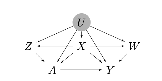
Figure 1: A proximal DAG

A key identification condition of proximal causal inference is that exists an outcome confounding bridge function $h^{\star}(w,a,x)$ that solves the following integral equation (Miao et al., 2018; Tchetgen Tchetgen et al., 2020)

$$\mathbb{E}[Y\mid Z,A,X]=\mathbb{E}\left[h^{\star}(W,A,X)\mid Z,A,X\right],\text{almost surely.}$$ (34)

Miao et al. (2023) then established sufficient conditions under which the CATE is nonparametrically identified by $\mathbb{E}(h(W,1,X)-h(W,0,X)|X)$.

Alternatively, Cui et al. (2023) considered an alternative identification strategy based on the following condition. There exists a treatment confounding bridge function $q^{\star}(z,a,x)$ that solves the following integral equation

$$\mathbb{E}\left[q^{\star}(Z,a,X)\mid W,A=a,X\right]=\frac{1}{\mathbb{P}(A=a\mid W,X)},\text{almost surely.}$$ (35)

Also see Deaner (2018) for a related condition. Cui et al. (2023) then established sufficient conditions under which the CATE is nonparametrically identified by $\mathbb{E}(Y(-1)^{1-A}q(Z,A,X)|X)$. Let $O=(X,Z,W,A,Y)$, Cui et al. (2023) derived the locally semiparametric efficient influence function for the marginal ATE (i.e. $\mathbb{E}[Y^{(1)}-Y^{(0)}]$) in a nonparametric model where one only assumes an outcome bridge function exists, at the submodel where both outcome and treatment confounding functions exist and are uniquely identified, but otherwise are unrestricted:

$$\mathrm{IF}_{\psi_{0}}(O;h^{\star},q^{\star})=-\mathbbm{1}\{A=a\}q^{\star}(Z,A,X)h^{\star}(W,A,X)$$ (36)

$$+\mathbbm{1}\{A=a\}Yq^{\star}(Z,A,X)+h^{\star}(W,a,X)-\psi_{0},$$ (37)

which falls in the mixed-bias class of influence functions (9) with $h_{0}(O_{h})=h^{\star}(W,A,X),q_{0}(O_{q})=q^{\star}(Z,A,X)$, $g_{1}(O)=-\mathbbm{1}\{A=a\},g_{2}(O)=\mathbbm{1}\{A=a\}Y,g_{3}(O)=1,g_{4}(O)=0$, and motivates the following FW-Learner of the CATE.

Proximal CATE FW-Learner estimator: Split the training data into two parts and train the nuisance functions $\widehat{q},\widehat{h}$ on the first split and define $\widehat{\tau}_{J}(x)$ to be the Forster–Warmuth estimator computed based on the data $\bigl{\{}(\widebar{\phi}_{J}(X_{i}),\widehat{I}(X_{i},A_{i},Y_{i},Z_{i},W_{i})),i\in\mathcal{I}_{2}\bigr{\}}$, where the pseudo-outcome $\widehat{I}$ is

$$\widehat{I}(O;\widehat{h},\widehat{q}) :=\bigl{\{}A\widehat{q}(Z,1,X)-(1-A)\widehat{q}(Z,0,X)\bigr{\}}\{Y-\widehat{h}(W,A,X)\}$$

$$\qquad\qquad+\widehat{h}(W,1,X)-\widehat{h}(W,0,X),$$ (38)

for any estimators $\widehat{h},\widehat{q}$ of the nuisance functions $h^{\star}$ and $q^{\star}$.

Write $H_{I}(X)=\mathbb{E}[\widehat{I}(O;\widehat{h},\widehat{q})|X]$, where the expectation is taken conditional on the first split of the training data. We have the following result.

Lemma 4.

The pseudo-outcome (38) has conditional bias :

$$H_{I}(x)-\tau^{\star}(x) =\mathbb{E}\biggl{[}A(h^{\star}-\widehat{h})(W,1,x)\bigl{(}\widehat{q}(Z,1,x)-q^{\star}(Z,1,x)\bigr{)}$$ (39)

$$\qquad\qquad-(1-A)(h^{\star}-\widehat{h})(W,0,x)\bigr{(}\widehat{q}(Z,0,x)-q^{\star}(Z,1,x)\bigr{)}\Bigm{|}X=x\biggr{]}.$$ (40)

This result directly follows from the mixed bias form (10) in the general class studied by Ghassami et al. (2022); its direct proof is deferred to Section S.7.3 of the supplement. Together with Corollary 1 yields a bound for the error of the FW-Learner $\widehat{\tau}_{J}$.

Theorem 6.

Let $\sigma^{2}$ be an upper bound on $\mathbb{E}[\widehat{I}^{2}(X,Z,W,A,Y)\mid X]$, the FW-Learner $\widehat{\tau}_{J}(x)$ satisfies:

$$\bigl{\|}\widehat{\tau}_{J}(X)-\tau^{\star}(X)\bigr{\|}_{2}\leq \sqrt{\frac{2\sigma^{2}J}{|\mathcal{I}_{2}|}}+\sqrt{2}\Bigl{\|}\sum_{j=J+1}^{\infty}\theta_{j}^{\star}\phi_{j}(X)\Bigr{\|}_{2}$$

$$+2(1+\sqrt{2})\min\Bigl{\{} \Bigl{\|}(\widehat{q}-q^{\star})(Z,1,X)\Bigr{\|}_{4}\Bigl{\|}\mathbb{E}\bigl{[}(\widehat{h}-h^{\star})(W,1,X)|Z,X\bigr{]}\Bigr{\|}_{4}$$

$$+\Bigl{\|}(\widehat{q}-q^{\star})(Z,0,X)\Bigr{\|}_{4}\Bigl{\|}\mathbb{E}\bigl{[}(\widehat{h}-h^{\star})(W,0,X)|Z,X\bigr{]}\Bigr{\|}_{4},$$

$$\Bigl{\|}\mathbb{E}\bigl{[}(\widehat{q}-q^{\star})(Z,1,X)\Bigm{|}W,X\bigr{]}\Bigr{\|}_{4}\Bigl{\|}(\widehat{h}-h^{\star})(W,1,X)\Bigr{\|}_{4}$$

$$+\Bigl{\|}\mathbb{E}\bigl{[}(\widehat{q}-q^{\star})(Z,0,X)\Bigm{|}W,X\bigr{]}\Bigr{\|}_{4}\Bigl{\|}(\widehat{h}-h^{\star})(W,0,X)\Bigr{\|}_{4}\Bigr{\}}.$$

The proof is in Section S.7.3 of the supplement. Note that the condition that $\sigma^{2}$ is bounded requires that $\widehat{h}_{0}$, $\widehat{h}_{1},\widehat{q}_{0}$ and $\widehat{q}_{1}$ are bounded. The rest of this section is concerned with estimation of the bridge functions $h^{\star}$ and $q^{\star}$.

Estimation of bridge functions $h^{\star}$ and $q^{\star}$:

Focusing primarily on $h^{\star}$, we note that integral equation (34) is a Fredholm integral equation of the first kind similar to integral equations of Section 3.2 on shadow variable FW-Learner, with corresponding kernel given by the conditional expectation operator $[T_{h}h](z,a,x)=\mathbb{E}[h(W_{i},A_{i},X_{i})\mid Z_{i}=z,A_{i}=a,X_{i}=x].$

Thus, minimax estimation of $h^{\star}$ follows from Chen and Christensen (2018) and Chen et al. (2021) attaining the rate $(n/\log n)^{-\alpha_{h}/(2(\alpha_{h}+\varsigma_{h})+d_{x}+d_{w}+1)}$ assuming $T_{h}$ is mildly ill-posed with exponent $\varsigma_{h}$; a corresponding adaptive minimax estimator that attains this rate is also given by the authors which does not require prior knowledge about $\alpha_{h}$ and $\varsigma_{h}$. See details given in Lemma 6 in the supplement. Analogous results also hold for $q^{\star}$ which can be estimated at the minimax rate of $(n/\log n)^{-\alpha_{q}/(2(\alpha_{q}+\varsigma_{q})+d_{x}+d_{z})}$ in the mildly ill-posed case, as established in Lemma 7 of the supplement, where $\alpha_{q}$ and $\varsigma_{q}$ are similarly defined. Without loss of generality, suppose that

$$\min\Bigl{\{} \Bigl{\|}(\widehat{q}-q^{\star})(Z,1,X)\Bigr{\|}_{4}\Bigl{\|}\mathbb{E}\bigl{[}(\widehat{h}-h^{\star})(W,1,X)|Z,X\bigr{]}\Bigr{\|}_{4}$$

$$+\Bigl{\|}(\widehat{q}-q^{\star})(Z,0,X)\Bigr{\|}_{4}\Bigl{\|}\mathbb{E}\bigl{[}(\widehat{h}-h^{\star})(W,0,X)|Z,X\bigr{]}\Bigr{\|}_{4},$$

$$\Bigl{\|}\mathbb{E}\bigl{[}(\widehat{q}-q^{\star})(Z,1,X)\Bigm{|}W,X\bigr{]}\Bigr{\|}_{4}\Bigl{\|}(\widehat{h}-h^{\star})(W,1,X)\Bigr{\|}_{4}$$

$$+\Bigl{\|}\mathbb{E}\bigl{[}(\widehat{q}-q^{\star})(Z,0,X)\Bigm{|}W,X\bigr{]}\Bigr{\|}_{4}\Bigl{\|}(\widehat{h}-h^{\star})(W,0,X)\Bigr{\|}_{4}\Bigr{\}}$$

$$=\Bigl{\|}(\widehat{q}-q^{\star})(Z,1,X)\Bigr{\|}_{4}\Bigl{\|}\mathbb{E}\bigl{[}(\widehat{h}-h^{\star})(W,1,X)|Z,X\bigr{]}\Bigr{\|}_{4}$$

$$+\Bigl{\|}(\widehat{q}-q^{\star})(Z,0,X)\Bigr{\|}_{4}\Bigl{\|}\mathbb{E}\bigl{[}(\widehat{h}-h^{\star})(W,0,X)|Z,X\bigr{]}\Bigr{\|}_{4}.$$

Further suppose that $\mu^{\star}(X,Z):=\mathbb{E}\bigl{[}h^{\star}(W,0,X)|Z,X\bigr{]}$ is $\alpha_{\mu}$-smooth, and $\Bigl{\|}\mathbb{E}\bigl{[}(\widehat{h}-h^{\star})(W,0,X)|Z,X\bigr{]}\Bigr{\|}_{4}$ matches the minimax rate of estimation for $\mu^{\star}(X,Z)$ with respect to the $L_{4}$-norm given by $n^{-\alpha_{\mu}/(2\alpha_{\mu}+d_{x}+d_{z})}$. Accordingly, Theorem 6, together with Lemma 6 and 7, leads to the following corollary.

Corollary 5.

Under the above conditions, together with the conditions of Lemma 6 and 7 in the supplement, and assuming that the integral equation with respect to the operator $T_{q}$ is mildly ill-posed, we have that:

$$\bigl{\|}\widehat{\tau}_{J}(X)-\tau^{\star}(X)\bigr{\|}_{2}\lesssim\sqrt{\frac{\sigma^{2}J}{n}}+J^{-\alpha_{\tau}/d_{x}}+ (n/\log n)^{-\alpha_{q}/(2(\alpha_{q}+\varsigma_{q})+d_{x}+d_{z})}n^{-\alpha_{\mu}/(2\alpha_{\mu}+d_{x}+d_{z})}.$$

A remark analogous to Remark 3.2 equally applies to Corollary 5. The result thus establishes conditions under which proximal the FW-Learner can estimate the CATE at the same rate as an oracle with access to bridge functions. This result appears to be completely new to the fast-growing literature on proximal causal inference.

5 Simulations

In this section, we study the finite sample performance of the proposed estimator focusing primarily on the estimation of the CATE via simulations. We consider a relatively simple data-generating mechanism which includes a covariate $X$ uniformly distributed on $[-1,1]$, a Bernoulli distributed treatment with conditional mean equal to $\pi^{\star}(x)=0.1+0.8\times\mathrm{sign}(x)$ and $\mu_{1}(x)=\mu_{0}(x)$ are equal to the piece-wise polynomial function defined on page 10 of Györfi et al. (2002). Therefore we are simulating under the null CATE model. Multiple methods are compared in the simulation study. Specifically, the simulation includes all four methods described in Section 4 of Kennedy (2020): 1. a plug-in estimator that estimates the regression functions $\mu_{0}^{\star}$ and $\mu_{1}^{\star}$ and takes the difference (called the T-Learner by Künzel et al. (2019), abbreviated as plugin below), 2. the X-Learner from Künzel et al. (2019) (xl), 3. the DR-Learner using smoothing splines from Kennedy (2020) (drl), and 4. an oracle DR Learner that uses the oracle (true) pseudo-outcome in the second-stage regression (oracle.drl), we compare these previous methods to 5. the FW-Learner with basic spline basis (FW_bs), and 6. the least squares series estimator with basic spline basis (ls_bs), where cross-validation is used to determine the number of basis functions to use for 5. and 6. Throughout, nuisance functions $\mu_{0}^{\star}$ and $\mu_{1}^{\star}$ are estimated using smoothing splines, and the propensity score $\pi^{\star}$ is estimated using logistic regression.

The top part of Figure 2 gives the mean squared error (MSE) for the six CATE estimators at training sample size $n=2000$, based on 500 simulations with MSE averaged over 500 independent test samples. The bottom part of Figure 2 gives the ratio of MSE of each competing estimator compared to the FW-Learner (the baseline method is FW_bs) across a range of convergence rates for the propensity score estimator $\widehat{\pi}$. The propensity score estimator is constructed as $\widehat{\pi}=\operatorname{expit}\left\{\operatorname{logit}(\pi)+\epsilon_{n}\right\}$, where $\epsilon_{n}\sim N\left(n^{-\alpha},n^{-2\alpha}\right)$ with varying convergence rate controlled by the parameter $\alpha$, so that $\operatorname{RMSE}(\widehat{\pi})\sim n^{-\alpha}$. The results demonstrate that, at least in the simulated setting, our FW-Learner attains the smallest mean squared error among all methods, approaching that of the oracle as the propensity score estimation error decreases (i.e., as the convergence rate increases). The performance of the FW-Learner and the least squares series estimator is visually challenging to distinguish in the figure; however closer numerical inspection confirms that the FW-Learner outperforms the least squares estimator.

To further illustrate the comparison between the proposed FW-Learner and the least squares estimator, we performed an additional simulation study focusing on these two estimators using two different sets of basis functions, in a simulation setting similar than the previous simulation, other than the covariate which we instead generate under a heavy-tailed distribution that is an equal probability mixture of a uniform distribution on $[-1,1]$ and a standard Gaussian distribution. The results are reported in Figure 3, for both FW-Learner (FW) and Least Squares (LS) estimators with basic splines (bs), natural splines (ns) and polynomial basis (poly). We report the ratio of MSE of all estimators against the FW-Learner with basic splines ($\text{FW}\_\text{bs}$). The sample size for the left-hand plot is $n=2000$, and $n=400$ for the right-hand plot. The FW-Learner consistently dominates the least squares estimator for any given choice of bases function in this more challenging setting. This additional simulation experiment demonstrates the robust of the FW-Learner against possible heavy-tailed distribution when compared to least-squares Learner.

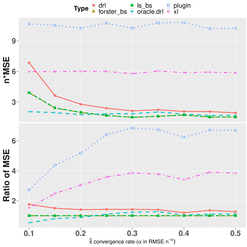
Figure 2: A comparison between different estimators, sample size $n=2000$—-Top figure shows $n\times\text{MSE}$ of each estimator; The bottom plot shows the ratio of MSE of different estimators compared to the proposed Forster–Warmuth estimator with basic splines (baseline). The MSE is averaged over 500 simulations.

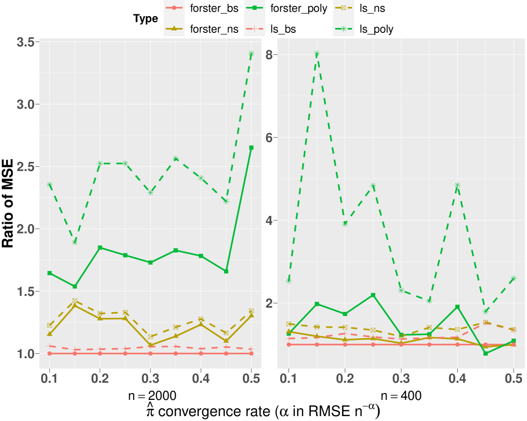
Figure 3: A comparison between FW and LS estimators with different basis for $X$ with heavy-tailed distribution, baseline method is the FW-Learner with basic splines ($\text{FW}\_\text{bs}$); Left: sample size $n=2000$; Right: $n=400$. The MSE is averaged over 500 simulations.

6 Data Application: CATE of Right Heart Catherization

We illustrate the proposed FW-Learner with an application of CATE estimation both assuming unconfoundedness and without making the assumption using proximal causal inference. Specifically, we reanalyze the Study to Understand Prognoses and Preferences for Outcomes and Risks of Treatments (SUPPORT) with the aim of evaluating the causal effect of right heart catheterization (RHC) during the initial care of critically ill patients in the intensive care unit (ICU) on survival time up to 30 days (Connors et al. (1996)). Tchetgen Tchetgen et al. (2020) and Cui et al. (2023) analyzed this dataset to estimate the marginal average treatment effect of RHC, using the proximal causal inference framework, with an implementation of a locally efficient doubly robust estimator, using parametric estimators of the bridge functions. Data are available on 5735 individuals, 2184 treated and 3551 controls. In total, 3817 patients survived and 1918 died within 30 days. The outcome Y is the number of days between admission and death or censoring at day 30. We include all 71 baseline covariates to adjust for potential confounding. To implement the FW-Learner under unconfoundedness, the nuisance functions $\pi^{\star}$, $\mu_{0}^{\star}$ and $\mu_{1}^{\star}$ are estimated using SuperLearner that includes both RandomForest and generalized linear model (GLM).

Variance of the FW-Learner:

In addition to producing an estimate of the CATE, one may wish to quantify uncertainty based on this estimate. We describe a simple approach for computing standard error for the CATE at a fixed value of $x$ and corresponding pointwise confidence intervals. The asymptotic guarantee of the confidence intervals for the least squares estimator is established in Newey (1997) and Belloni et al. (2015) under some conditions. Because the FW-Learner is asymptotically equivalent to the Least-squares estimator, the same variance estimator as that of the least squares series estimator may be used to quantify uncertainty about the FW-Learner. Recall that the Least-squares estimator is given by $\widebar{\phi}(x)^{\top}\bigl{[}\sum_{i}(\widebar{\phi}(X_{i})\widebar{\phi}(X_{i})^{\top}\bigr{]}^{-1}\bigl{\{}\sum_{i}\widebar{\phi}(X_{i})\widehat{I}_{i}\bigr{\}}$, the latter has variance $\widebar{\phi}(x)^{\top}\bigl{[}\sum_{i}(\widebar{\phi}(X_{i})\widebar{\phi}(X_{i})^{\top}\bigr{]}^{-1}\widebar{\phi}(x)\times\sigma^{2}(\widehat{I})$, where $\sigma^{2}(\widehat{I})$ is the variance of the pseudo-outcome $\widehat{I}$; where we have implicitly assumed homoscedasticity, i.e. that the variance of $(\widehat{I})$ is independent of $X$. Hence,

$$\mathrm{var}(\widehat{\tau}(x))\approx\widebar{\phi}(x)^{\top}\bigl{[}\sum_{i}(\widebar{\phi}(X_{i})\widebar{\phi}(X_{i})^{\top}\bigr{]}^{-1}\widebar{\phi}(x)\times\sigma^{2}(\widehat{I}).$$ (41)

Similar to Tchetgen Tchetgen et al. (2020) and Cui et al. (2023), our implementation of the Proximal FW-Learner specified baseline covariates $(\text{age, sex, cat1 coma}$, cat2 coma, dnr1, surv2md1, aps1) for confounding adjustment; as well as treatment and outcome confounding proxies $Z=(\text{pafi1},\text{paco21})$ and $W=(\text{ph1},\text{hema1})$. Confounding bridge functions were estimated nonparametrically using the adversarial reproducing kernel Hilbert spaces (RKHS) learning approach of Ghassami et al. (2022). The estimated CATE and corresponding pointwise 95 percent confidence intervals are reported in Figure 4 as a function of the single variable measuring the 2-month model survival prediction at data 1 (surv2md1), for both approaches, each using both splines and polynomials. Cross-validation was used throughout to select the number of knots for splines and the degree of the polynomial bases, respectively. The results are somewhat consistent for both bases functions, and suggest at least under unconfoundedness conditions that high risk patients likely benefited most from RHC, while low risk patients may have been adversely impacted by RHC. In contrast, The Proximal FW-Learner produced a more attenuated CATE estimate, which however found that RHC was likely harmful for low risk patients. Interestingly, these analyses provide important nuances to results reported in the original analysis of Connors et al. (1996) and the more recent analysis of Tchetgen Tchetgen et al. (2020) which concluded that RHC was harmful on average on the basis of the ATE.

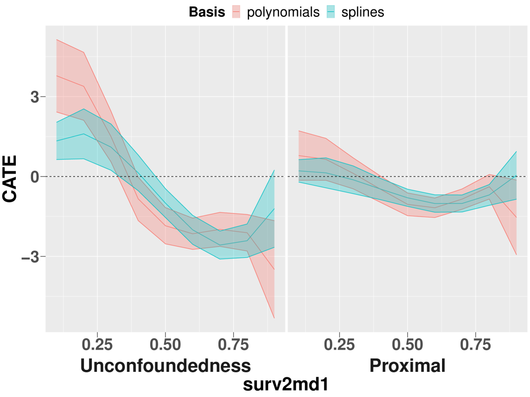
Figure 4: CATE estimation with $95\%$ confidence interval produced by the FW-Learner using polynomial and spline basis. Left: under unconfoundedness; Right: in proximal causal inference setting.

7 Discussion

This paper has proposed a novel nonparametric series estimator of regression functions that requires minimal assumptions on covariates and bases functions. Our method builds on the Forster–Warmuth estimator, which incorporates weights based on the leverage score $h_{n}(x)=x^{\top}(\sum_{i=1}^{n}X_{i}X_{i}^{\top}+xx^{\top})^{-1}x$, to obtain predictions that can be significantly more robust relative to standard least-squares, particularly in small to moderate samples. Importantly, the FW-Learner is shown to satisfy an oracle inequality with its excess risk bound having the same order as $J\sigma^{2}/n$, requiring only the relatively mild assumption of bounded outcome second moment ($\mathbb{E}[Y^{2}\mid x]\leq\sigma^{2}$). Recent works (Mourtada (2019), Vaškevičius and Zhivotovskiy (2023)) investigate the potential for the risk of standard least-squares to become unbounded when leverage scores are uneven and correlated with the residual noise of the model. By adjusting the predictions at high-leverage points, which are most likely to lead to an unstable estimator, the Forster–Warmuth estimator mitigates the shortcomings of the least squares estimator and achieves oracle bounds even for unfavorable distributions when least squares estimation fails. In fact, the Forster–Warmuth algorithm leads to the only known exact oracle inequality without imposing any assumptions on the covariates. This is a key strength of the FW-Learner we fully leverage in the context of nonparametric series estimation to obviate imposing unnecessary conditions on the basis functions.

Another major contribution we make is to propose a general method for counterfactual nonparametric regression via series estimation in settings where the outcome may be missing. Specifically, we generalize the FW-Learner using a generic pseudo-outcome that serves as substitution for the missing response and we characterize the extent to which accuracy of the pseudo-outcome can potentially impact the estimator’s ability to match the oracle minimax rate of estimation on the MSE scale. We then provide a generic approach for constructing a pseudo-outcome with “small bias” property for a large class of counterfactual regression problems, based on a doubly robust influence functions of the functional obtained via marginalizing the counterfactual regression in view. This insight provides a constructive solution to the counterfactual regression problem and offers a unified solution to several open nonparametric regression problems in both missing data and causal inference literatures. The versatility of the approach is demonstrated by considering estimation of nonparametric regression when the outcome may be missing at random; or when the outcome may be missing not at random by leveraging a shadow variable. As well as by considering estimation of the CATE under standard unconfoundedness conditions; and when hidden confounding bias cannot be ruled out on the basis of measured covariates, however proxies of unmeasured factors are available that can be leveraged using proximal causal inference framework. While some of these settings such as CATE under unconfoundedness have been studied extensively, others such as the CATE under proximal causal inference have only recently developed.

Overall, this paper brings together aspects of traditional linear models, nonparametric models and modern literature of semiparametric theory, with applications in different contexts. This marriage of classical and modern techniques is in similar spirit as recent frameworks such as Orthogonal Learning (Foster and Syrgkanis, 2019), however our assumptions and approach appear to be fundamentally different in that, at least for specific examples considered herein, our assumptions are somewhat weaker yet lead to a form of oracle optimality. We nevertheless believe that both frameworks open the door to many future exciting directions to explore. A future line of investigation might be to extend the estimator using more accurate pseudo-outcomes of the unobserved response using recent theory on higher order influence functions (Robins et al., 2008, 2017), along the lines of Kennedy et al. (2022) who constructs minimax estimators of the CATE under unconfoundness conditions and weaker smoothness conditions on the outcome and propensity score models, however requiring considerable restrictions on the covariate distribution.Another interesting direction is the potential application of our methods to more general missing data settings, such as monotone or nonmonotone coarsening at random settings (Robins et al., 1994; Laan and Robins, 2003; Tsiatis, 2006), and corresponding coarsening not at random settings, e.g. Robins et al. (2000), Tchetgen Tchetgen et al. (2018), Malinsky et al. (2022). We hope the current manuscript provides an initial step towards solving this more challenging class of problems and generates both interest and further developments in these fundamental directions.

Supplement to “Forster–Warmuth Counterfactual Regression: A Unified Approach”

S.1 More Examples of Pseudo-outcome

S.1.1 Conditional Quantile Causal Effect

Suppose $F(Y|X,A)$ is differentiable on the support of $Y$; we consider construction of the pseudo-outcome for the conditional quantile causal effect under unconfoundedness

$$\beta\left(X;\eta\right)=F_{Y|A,X}^{-1}\left(q|A=1,X\right)-F_{Y|A,X}^{-1}\left(q|A=0,X\right)$$

In which case

$$\psi=\mathbb{E}_{X}\left\{F_{Y|A,X}^{-1}\left(q|A=1,X\right)-F_{Y|A,X}^{-1}\left(q|A=0,X\right)\right\}$$

and the EIF of the latter is given by

$$\nabla_{t}\psi_{t}=\nabla_{t}\mathbb{E}_{X,t}\left\{F_{Y|A,X,t}^{-1}\left(q|A=1,X\right)-F_{Y|A,X,t}^{-1}\left(q|A=0,X\right)\right\}$$

This requires finding $R(O;\eta)$ such that

$$\mathbb{E}_{O|X}\left\{\nabla_{t}F_{Y|A,X,t}^{-1}\left(q|A=1,X\right)-F_{Y|A,X,t}^{-1}\left(q|A=0,X\right)|X;\eta\right\}=\mathbb{E}\left\{R(O;\eta)S(O)|X;\eta\right\}$$

note that for $\theta_{t}\left(X\right)=F_{Y|A,X,t}^{-1}\left(q|A=1,X\right),$

$$\nabla_{t}q = \nabla_{t}\int_{0}^{\theta_{t}\left(X\right)}f_{t}\left(y|A=1,X\right)$$

$$= \nabla_{t}\theta_{t}\left(X\right)f_{t}\left(\theta_{t}\left(X\right)|A=1,X\right)+\mathbb{E}\left\{I\left(Y<\theta_{t}\left(X\right)-q\right)S\left(Y|A=1,X\right)\right\}$$

$$\nabla_{t}F_{Y|A,X,t}^{-1}\left(q|A=1,X\right)$$

$$= \frac{\nabla_{t}F_{Y|A,X,t}\left(q|A=1,X\right)}{f\left(F_{Y|A,X,t}^{-1}\left(q|A=1,X\right)|A=1,X\right)}$$

$$= -\frac{\mathbb{E}\left\{\left(I\left(Y\leq F_{Y|A,X,t}^{-1}\left(q|A=1,X\right)\right)-q\right)S(Y|A=1,X)|X;\eta\right\}}{f\left(F_{Y|A,X,t}^{-1}\left(q|A=1,X\right)|A=1,X\right)}$$

$$= -\mathbb{E}\left\{\frac{I(A=1)\left(I\left(Y\leq F_{Y|A,X,t}^{-1}\left(q|A,X\right)\right)-q\right)}{f(A|X)f\left(F_{Y|A,X,t}^{-1}\left(q|A,X\right)|A,X\right)}S(Y|A,X)|X;\eta\right\}$$

$$= -\mathbb{E}\left\{\frac{I(A=1)\left(I\left(Y\leq F_{Y|A,X,t}^{-1}\left(q|A,X\right)\right)-q\right)}{f(A|X)f\left(F_{Y|A,X,t}^{-1}\left(q|A,X\right)|A,X\right)}S(O)|X;\eta\right\}$$

Likewise

$$\nabla_{t}F_{Y|A,X,t}^{-1}\left(q|A=0,X\right)$$

$$= \frac{\nabla_{t}F_{Y|A,X,t}\left(q|A=0,X\right)}{f\left(F_{Y|A,X,t}^{-1}\left(q|A=0,X\right)|A=0,X\right)}$$

$$= \frac{\mathbb{E}\left\{\left(I\left(Y\leq F_{Y|A,X,t}^{-1}\left(q|A=0,X\right)\right)-q\right)S(Y|A=0,X)|X;\eta\right\}}{f\left(F_{Y|A,X,t}^{-1}\left(q|A=0,X\right)|A=0,X\right)}$$

$$= \mathbb{E}\left\{\frac{I(A=0)\left(I\left(Y\leq F_{Y|A,X,t}^{-1}\left(q|A,X\right)\right)-q\right)}{f(A|X)f\left(F_{Y|A,X,t}^{-1}\left(q|A,X\right)|A,X\right)}S(Y|A,X)|X;\eta\right\}$$

$$= \mathbb{E}\left\{\frac{I(A=0)\left(I\left(Y\leq F_{Y|A,X,t}^{-1}\left(q|A,X\right)\right)-q\right)}{f(A|X)f\left(F_{Y|A,X,t}^{-1}\left(q|A,X\right)|A,X\right)}S(O)|X;\eta\right\}$$

Therefore

$$\nabla_{t}\psi_{t}=\mathbb{E}\left[\left\{\begin{array}[]{c}-\frac{I(A=1)\left(I\left(Y\leq F_{Y|A,X,t}^{-1}\left(q|A,X\right)\right)-q\right)}{f(A|X)f\left(F_{Y|A,X,t}^{-1}\left(q|A,X\right)|A,X\right)}\\ +\frac{I(A=0)\left(I\left(Y\leq F_{Y|A,X,t}^{-1}\left(q|A,X\right)\right)-q\right)}{f(A|X)f\left(F_{Y|A,X,t}^{-1}\left(q|A,X\right)|A,X\right)}\\ +F_{Y|A,X}^{-1}\left(q|A=1,X\right)-F_{Y|A,X}^{-1}\left(q|A=0,X\right)\end{array}\right\}S\left(O\right)\right]$$

and the pseudo-outcome is given by

$$I = R(O;\eta)+r(O;\eta)$$

$$= \frac{I(A=1)\left(I\left(Y\leq F_{Y|A,X,t}^{-1}\left(q|A,X\right)\right)-q\right)}{f(A|X)f\left(F_{Y|A,X,t}^{-1}\left(q|A,X\right)|A,X\right)}$$

$$-\frac{I(A=0)\left(I\left(Y\leq F_{Y|A,X,t}^{-1}\left(q|A,X\right)\right)-q\right)}{f(A|X)f\left(F_{Y|A,X,t}^{-1}\left(q|A,X\right)|A,X\right)}$$

$$+F_{Y|A,X}^{-1}\left(q|A=1,X\right)-F_{Y|A,X}^{-1}\left(q|A=0,X\right)$$

S.1.2 CATE in Generalized Linear Model

Consider the CATE in a GLM of the form

$$\beta\left(X;\eta\right)=g^{-1}\left\{\mathbb{E}\left(Y|A=1,X\right)\right\}-g^{-1}\left\{\mathbb{E}\left(Y|A=0,X\right)\right\}$$

for known link function $g.$ In which case

$$\psi=\mathbb{E}_{X}\left\{g^{-1}\left\{\mathbb{E}\left(Y|A=1,X\right)\right\}-g^{-1}\left\{\mathbb{E}\left(Y|A=0,X\right)\right\}\right\},$$

and the EIF of the latter is given by

$$\nabla_{t}\psi_{t}=\nabla_{t}\mathbb{E}_{X,t}\left\{g^{-1}\left\{\mathbb{E}_{t}\left(Y|A=1,X\right)\right\}-g^{-1}\left\{\mathbb{E}_{t}\left(Y|A=0,X\right)\right\}\right\}.$$

This requires finding $R(O;\eta)$ such that

$$\mathbb{E}_{O|X}\left\{\nabla_{t}g^{-1}\left\{\mathbb{E}_{t}\left(Y|A=1,X\right)\right\}-g^{-1}\left\{\mathbb{E}_{t}\left(Y|A=0,X\right)\right\}|X;\eta\right\}=\mathbb{E}\left\{R(O;\eta)S(O|X)|X;\eta\right\}.$$

We have that

$$\mathbb{E}_{O|X}\left\{\nabla_{t}g^{-1}\left\{\mathbb{E}_{t}\left(Y|A=1,X\right)\right\}-g^{-1}\left\{\mathbb{E}_{t}\left(Y|A=0,X\right)\right\}|X;\eta\right\}$$

$$= \mathbb{E}_{O|X}\left\{\frac{\nabla_{t}\left\{\mathbb{E}_{t}\left(Y|A=1,X\right)\right\}}{g^{\prime}\left\{g^{-1}\left\{\mathbb{E}_{t}\left(Y|A=1,X\right)\right\}\right\}}-\frac{\nabla_{t}\left\{\mathbb{E}_{t}\left(Y|A=0,X\right)\right\}}{g^{\prime}\left\{g^{-1}\left\{\mathbb{E}_{t}\left(Y|A=0,X\right)\right\}\right\}}|X;\eta\right\}$$

$$= \mathbb{E}_{O|X}\left\{\left[\frac{I\left(A=1\right)\left\{Y-\mathbb{E}\left(Y|A,X\right)\right\}}{f\left(A|X\right)g^{\prime}\left\{g^{-1}\left\{\mathbb{E}\left(Y|A,X\right)\right\}\right\}}-\frac{I\left(A=0\right)\left\{Y-\mathbb{E}\left(Y|A,X\right)\right\}}{f\left(A|X\right)g^{\prime}\left\{g^{-1}\left\{\mathbb{E}\left(Y|A,X\right)\right\}\right\}}\right]S(O|X)|X;\eta\right\}.$$

Therefore,

$$I = R(O;\eta)+r(O;\eta)$$

$$= \frac{\left(-1\right)^{1-A}\left\{Y-\mathbb{E}\left(Y|A,X\right)\right\}}{f\left(A|X\right)g^{\prime}\left\{g^{-1}\left\{\mathbb{E}\left(Y|A,X\right)\right\}\right\}}+g^{-1}\left\{\mathbb{E}\left(Y|A=1,X\right)\right\}-g^{-1}\left\{\mathbb{E}\left(Y|A=0,X\right)\right\},$$

which in the case of identity link recovers the CATE pseudo-outcome. In the case of log link $g^{\prime}\left(\cdot\right)=g\left(\cdot\right)=\exp\left(\cdot\right)$, therefore

$$I=\frac{\left(-1\right)^{1-A}\left\{Y-\mathbb{E}\left(Y|A,X\right)\right\}}{f\left(A|X\right)\mathbb{E}\left(Y|A,X\right)}+\log\left\{\mathbb{E}\left(Y|A=1,X\right)\right\}-\log\left\{\mathbb{E}\left(Y|A=0,X\right)\right\}.$$

Likewise, consider the GLM with the logit link for binary $Y$

$$\psi=\mathbb{E}_{X}\left[\text{logit}\mathbb{E}\left(Y|A=1,X\right)-\text{logit}\mathbb{E}\left(Y|A=0,X\right)\right],$$

and the EIF of the latter is given by

$$\nabla_{t}\psi_{t}=\nabla_{t}\mathbb{E}_{X,t}\left\{\underset{\beta\left(X;\eta\right)}{\underbrace{\text{logit}\left\{\mathbb{E}_{t}\left(Y|A=1,X\right)\right\}-\text{logit}\left\{\mathbb{E}_{t}\left(Y|A=0,X\right)\right\}}}\right\}.$$

Note that $g(b)=\exp\left(b\right)/\left(1+\exp(b)\right)$ and $g^{\prime}(b)=\exp\left(b\right)/\left(1+\exp(b)\right)^{2}$, $g^{-1}\left(p\right)=\log({p}/{(1-p)}).$ Therefore

$$I = R(O;\eta)+r(O;\eta)$$

$$= \frac{\left(-1\right)^{1-A}\left\{Y-\mathbb{E}\left(Y|A,X\right)\right\}}{f\left(A|X\right)g^{\prime}\left\{g^{-1}\left\{\mathbb{E}\left(Y|A,X\right)\right\}\right\}}+g^{-1}\left\{\mathbb{E}\left(Y|A=1,X\right)\right\}-g^{-1}\left\{\mathbb{E}\left(Y|A=0,X\right)\right\}$$

$$= \frac{\left(-1\right)^{1-A}\left\{Y-\mathbb{E}\left(Y|A,X\right)\right\}}{f\left(A|X\right)\mathbb{P}\left(Y=1|A,X\right)\left(1-\mathbb{P}\left(Y=1|A,X\right)\right)}+\log\left\{\frac{\mathbb{P}\left(Y=1|A=1,X\right)}{\mathbb{P}\left(Y=0|A=1,X\right)}\right\}$$

$$\quad- \log\left\{\frac{\mathbb{P}\left(Y=1|A=0,X\right)}{\mathbb{P}\left(Y=0|A=0,X\right)}\right\}$$

$$= \frac{\left(-1\right)^{A+Y}}{f(Y,A|X)}+\log\left\{\frac{\mathbb{P}\left(Y=1|A=1,X\right)}{\mathbb{P}\left(Y=0|A=1,X\right)}\right\}-\log\left\{\frac{\mathbb{P}\left(Y=1|A=0,X\right)}{\mathbb{P}\left(Y=0|A=0,X\right)}\right\}.$$

The leading term above was obtained Tchetgen Tchetgen et al. (2010) as an influence function in a semiparametric odds ratio model.

S.1.3 Dose Response with Continuous Treatment (No confounding)

Consider the case of continuous treatment $A$ where we aim to estimate the dose response curve $E\left(Y_{a}\right)$

under unconfoundedness of $A$ given $L$

$$\beta\left(a\right)=\mathbb{E}\left(Y_{a}\right)=\mathbb{E}_{L}\left\{\mathbb{E}\left(Y|A=a,L\right)\right\}.$$

As the outer-expectation can be estimated nonparametrically at rate root-n, its uncertainty is negligible relative to that of $\mathbb{E}\left(Y|A=a,L\right)$ and therefore we may consider the semiparametric model where $f(L)\$is known, in which case under an arbitrary corresponding submodel :

$$\nabla_{t}\mathbb{E}_{t}\left\{r(O;\eta_{t})|X=x\right\} = \nabla_{t}r(O;\eta_{t})=\nabla_{t}\sum_{l}\mathbb{E}_{t}\left(Y|X=x,l\right)f\left(l\right)$$

$$= \sum_{l}\nabla_{t}\mathbb{E}_{t}\left(Y|X=x,l\right)f\left(l\right)$$

$$= \sum_{l}\mathbb{E}\left(\left\{Y-\mathbb{E}\left(Y|X=x,l\right)\right\}S\left(Y|X,l\right)|X=x,l\right)f\left(l\right)$$

$$= \sum_{l}\mathbb{E}\left(\left\{Y-\mathbb{E}\left(Y|X=x,l\right)\right\}\frac{f\left(l\right)}{f\left(l|X=x\right)}S\left(Y|X,l\right)|X=x,l\right)f\left(l|X=x\right)$$

$$= \mathbb{E}\left[\left\{Y-\mathbb{E}\left(Y|X,L\right)\right\}\frac{f\left(X\right)}{f\left(X|L\right)}S\left(O\right)|X=x\right].$$

Therefore,

$$I = R(O;\eta)+r(O;\eta)$$

$$= \left\{Y-\mathbb{E}\left(Y|X,L\right)\right\}\frac{f\left(X\right)}{f\left(X|L\right)}+\sum_{l}\mathbb{E}\left(Y|X,l\right)f\left(l\right),$$

recovering the pseudo-outcome of Kennedy et al. (2017).

S.1.4 Dose Response for Continuous Treatment (Confounding)

Consider the case of continuous treatment $A$ where we aim to estimate the dose response curve $\mathbb{E}\left(Y_{a}\right)$

under endogeneity, given treatment and outcome proxies $Z,W$ and covariates $L,$ using the proximal causal inference framework of Miao et al. (2018) and Tchetgen Tchetgen et al. (2020),

$$\beta\left(a\right)=\mathbb{E}\left(Y_{a}\right)=\mathbb{E}_{L}\left\{h\left(W,a,L\right)\right\}.$$

As the outer-expectation can be estimated nonparametrically at rate root-n, its uncertainty is negligible relative to that of $h\left(W,a,L\right)$, and therefore we may consider the semiparametric model where $f(w,L)\$is known. Thus, taking

$$r(O;\eta)=\sum_{w,l}h\left(w,a,l\right)f\left(w,l\right),$$

in which case under an arbitrary corresponding submodel:

$$\nabla_{t}\mathbb{E}_{t}\left\{r(O;\eta_{t})|A=a\right\} = \nabla_{t}r(O;\eta_{t})=\nabla_{t}\sum_{w,l}h\left(w,a,l\right)f\left(w,l\right)$$

$$= \sum_{l,w}\nabla_{t}h_{t}\left(w,a,l\right)f\left(l,w\right)$$

$$= \sum_{l,w}\nabla_{t}h_{t}\left(w,a,l\right)\frac{f\left(l,w\right)}{f\left(l,w|a\right)}f\left(l,w|a\right)$$

$$= \sum_{l,w}\nabla_{t}h_{t}\left(w,a,l\right)\frac{f\left(a\right)}{f\left(a|l,w\right)}f\left(l,w|a\right)$$

$$= \sum_{l,w}\nabla_{t}h_{t}\left(w,a,l\right)\mathbb{E}\left[q\left(a,Z,l\right)|l,w,a\right]f\left(l,w|a\right)$$

$$= \sum_{l,w,z}\nabla_{t}h_{t}\left(w,a,l\right)q\left(a,z,l\right)f\left(z,l,w|a\right)$$

$$= \sum_{l,z}\mathbb{E}\left[\nabla_{t}h_{t}\left(W,a,l\right)|a,z,l\right]q\left(a,z,l\right)f\left(z,l|a\right)$$

$$= \sum_{l,z}\mathbb{E}\left[\left\{Y-h\left(W,a,l\right)\right\}S\left(Y,W|a,z,l\right)|a,z,l\right]q\left(a,z,l\right)f\left(z,l|a\right)$$

$$= \mathbb{E}\left[\left\{Y-h\left(W,A,L\right)\right\}q\left(A,Z,L\right)S\left(Y,W|A,Z,L\right)|A=a\right]$$

$$= \mathbb{E}\left[\left\{Y-h\left(W,A,L\right)\right\}q\left(A,Z,L\right)S\left(O\right)|A=a\right].$$

Therefore,

$$I = R(O;\eta)+r(O;\eta)$$

$$= \left\{Y-h\left(W,A,L\right)\right\}q\left(A,Z,L\right)+\sum_{w,l}h\left(w,A,l\right)f\left(w,l\right),$$

generalizing the pseudo-outcome approach of Kennedy et al. (2017) to the Proximal inference framework with continuous treatment.

S.1.5 CATE under IV Identification

In this example, we consider the CATE under IV identification. In this vein, let $A$ denote a binary treatment, $Z$ denote a binary instrumental variable, $L$ measured covariates, $Y$ the outcome variable. Under identification conditions given in Wang and Tchetgen Tchetgen (2018), we have that

$$\beta\left(X;\eta\right)=\mathbb{E}\left\{Y_{a=1}-Y_{a=0}|L\right\}=\frac{\mathbb{E}\left(Y|Z=1,L\right)-\mathbb{E}\left(Y|Z=0,L\right)}{\mathbb{E}\left(A|Z=1,L\right)-\mathbb{E}\left(A|Z=0,L\right)}.$$

Let

$$\delta_{A}\left(L\right) \equiv \mathbb{E}\left(A|Z=1,L\right)-\mathbb{E}\left(A|Z=0,L\right);$$

$$r(O;\eta) = \frac{\mathbb{E}\left(Y|Z=1,L\right)-\mathbb{E}\left(Y|Z=0,L\right)}{\mathbb{E}\left(A|Z=1,L\right)-\mathbb{E}\left(A|Z=0,L\right)}.$$

Then following Wang and Tchetgen Tchetgen (2018), one has that

$$\nabla_{t}\mathbb{E}_{t}\left\{r(O;\eta_{t})|X=x\right\} = \nabla_{t}r(O;\eta_{t})$$

$$= \mathbb{E}\left\{R(O;\eta,\beta\left(\eta\right))S\left(O\right)|X=x\right\},$$

where

$$R(O;\eta,\beta\left(\eta\right)=\frac{2Z-1}{f\left(Z|X\right)}\frac{\left\{Y-A\beta\left(X;\eta\right)-\mathbb{E}\left(Y|Z=0,L\right)+\mathbb{E}\left(A|Z=0,L\right)\beta\left(X;\eta\right)\right\}}{\delta_{A}\left(L\right)}.$$

Therefore,

$$I = R(O;\eta)+r(O;\eta)$$

$$= \frac{2Z-1}{f\left(Z|X\right)}\frac{\left\{Y-A\beta\left(X;\eta\right)-\mathbb{E}\left(Y|Z=0,L\right)+E\left(A|Z=0,L\right)\beta\left(X;\eta\right)\right\}}{\delta_{A}\left(L\right)}+\beta\left(X;\eta\right).$$

S.1.6 CATE under IV Identification 2

We next consider the CATE for the Complier under IV identification. In this vein, under identification conditions given in Angrist et al. (1996), we have that

$$\beta\left(X;\eta\right)=\mathbb{E}\left\{Y_{a=1}-Y_{a=0}|A_{1}>A_{0},L\right\}=\frac{\mathbb{E}\left(Y|Z=1,L\right)-\mathbb{E}\left(Y|Z=0,L\right)}{\mathbb{E}\left(A|Z=1,L\right)-\mathbb{E}\left(A|Z=0,L\right)}.$$

in which case the above results continue to hold. Likewise, under identification conditions given by Robins et al. (1994), the CATE for the treated is given by the same formula

$$\beta\left(X;\eta\right)=\mathbb{E}\left\{Y_{a=1}-Y_{a=0}|A=1,L\right\}=\frac{\mathbb{E}\left(Y|Z=1,L\right)-\mathbb{E}\left(Y|Z=0,L\right)}{\mathbb{E}\left(A|Z=1,L\right)-\mathbb{E}\left(A|Z=0,L\right)}.$$

S.2 Proof of Theorem 1 and Corollary 1

Proof of Theorem 1.

Theorem $6.2$ of Forster and Warmuth (2002) implies that

$$\mathbb{E}\Bigl{[}\bigl{(}Y-\widehat{m}_{J}(X)\bigr{)}^{2}\Bigr{]} \leq\inf_{\beta_{1},\ldots,\beta_{J}}\mathbb{E}\Bigl{[}\bigl{(}Y-\sum_{j=1}^{J}\beta_{j}\phi_{j}(X)\bigr{)}^{2}\Bigr{]}+\frac{2\sigma^{2}J}{n}$$

$$=\mathbb{E}[(Y-m^{\star}(X))^{2}]+\inf_{\beta_{1},\ldots,\beta_{J}}\mathbb{E}\Bigl{[}\bigl{(}m^{\star}(X)-\sum_{j=1}^{J}\beta_{j}\phi_{j}(X)\bigr{)}^{2}\Bigr{]}+\frac{2\sigma^{2}J}{n},$$

where $\sigma^{2}$ is an upper bound on $\mathbb{E}\bigl{[}Y^{2}|X\bigr{]}$. To control the second term above, observe that if $f_{X}(\cdot)$ is the density of $X$ with respect to $\mu$, then for any $(\beta_{1},\ldots,\beta_{J})$,

$$\mathbb{E}\Bigl{[}\bigl{(}m^{\star}(X)-\sum_{j=1}^{J}\beta_{j}\phi_{j}(X)\bigr{)}^{2}\Bigr{]}=\int\bigl{(}m^{\star}(x)-\sum_{j=1}^{J}\beta_{j}\phi_{j}(x)\bigr{)}^{2}f_{X}(x)d\mu(x)\leq\kappa\left\|m^{\star}-\sum_{j=1}^{J}\beta_{j}\phi_{j}\right\|_{L_{2}(\mu)}^{2}.$$

Hence, the infimum of the left-hand side over all $\beta_{1},\ldots,\beta_{J}$ is bounded by $\kappa(E_{J}^{\Psi}(m^{\star}))^{2}$. Finally, note that $m^{\star}(\cdot)$ being the conditional mean of $Y$ given $X$ implies $\mathbb{E}\bigl{[}(Y-\widehat{m}_{J}(X))^{2}\bigr{]}-\mathbb{E}\bigl{[}(Y-m^{\star}(X))^{2}\bigr{]}=\mathbb{E}\bigl{[}(\widehat{m}_{J}(X)-m^{\star}(X))^{2}\bigr{]}$. Therefore,

$$\mathbb{E}\Bigl{[}\bigl{(}\widehat{m}_{J}(X)-m^{\star}(X)\bigr{)}^{2}\Bigr{]}\leq\frac{2\sigma^{2}J}{n}+\kappa(E_{J}^{\Psi}(m^{\star}))^{2}.$$

To prove the second part of Theorem 1, note that $m^{\star}\in\mathcal{F}(\Psi,\Gamma)$ implies that $E_{J}^{\Psi}(m^{\star})\leq\gamma_{J}$ and by definition of $J_{n}$, $\gamma_{J_{n}}^{2}\leq\sigma^{2}J_{n}/n$. These inequalities imply that

$$\|\widehat{m}_{J_{n}}-m^{\star}\|_{2}^{2}\leq\frac{2\sigma^{2}J_{n}}{n}+\kappa\gamma_{J_{n}}\leq\frac{2\sigma^{2}J_{n}}{n}+\kappa\frac{\sigma^{2}J_{n}}{n}=(2+\kappa)\frac{\sigma^{2}J_{n}}{n}.$$

∎

Proof of Corollary 1.

Applying the result for Forster–Warmuth estimator (from Theorem $6.2$ Forster and Warmuth (2002)), this gives

$$\mathbb{E}\Bigl{[}\bigl{(}\widehat{f}(O)-\widehat{m}_{J}(X)\bigr{)}^{2}\big{|}\widehat{f}\Bigr{]}\leq\inf_{\theta\in\mathbb{R}^{J}}\mathbb{E}\Bigl{[}\bigl{(}\widehat{f}(O)-\theta^{\top}\bar{\phi}_{J}(X)\Bigr{)}^{2}\big{|}\widehat{f}\Bigr{]}+\frac{2\sigma^{2}J}{|\mathcal{I}_{2}|},$$ (E.1)

where $\sigma^{2}=\sup_{x}\mathbb{E}[\widehat{f}^{2}(O)|X=x,\widehat{f}]$. Now write $m^{\star}(x)=\sum_{j=1}^{\infty}\theta_{j}^{\star}\phi_{j}(x),$ and taking $(\theta_{1}^{\star},\ldots,\theta_{J}^{\star})$ for the infimum, we conclude

$$\inf_{\theta\in\mathbb{R}^{J}}\mathbb{E}\Bigl{[}\bigl{(}\widehat{f}(O)-\theta^{\top}\bar{\phi}_{J}(X)\bigr{)}^{2}\big{|}\widehat{f}\Bigr{]} \leq\mathbb{E}\Bigl{[}\bigl{(}\widehat{f}(O)-\sum_{j=1}^{J}\theta_{j}^{\star}\phi_{j}(X)\bigr{)}^{2}\big{|}\widehat{f}\Bigr{]}$$

$$=\mathbb{E}\Bigl{[}\bigl{(}\widehat{f}(O)-H_{f}(X)\bigr{)}^{2}\big{|}\widehat{f}\Bigr{]}+\mathbb{E}\Bigl{[}\bigl{(}H_{f}(X)-\sum_{j=1}^{J}\theta_{j}^{\star}\phi_{j}(X)\bigr{)}^{2}\big{|}\widehat{f}\Bigr{]}$$

$$\leq\mathbb{E}\Bigl{[}\bigl{(}\widehat{f}(O)-H_{f}(X)\bigr{)}^{2}\big{|}\widehat{f}\Bigr{]}+2\mathbb{E}\Bigl{[}\bigl{(}H_{f}(X)-m^{\star}(X)\bigr{)}^{2}\big{|}\widehat{f}\Bigr{]}$$

$$\quad+2\mathbb{E}\Bigl{[}\bigl{(}m^{\star}(X)-\sum_{j=1}^{J}\theta_{j}^{\star}\phi_{j}(X)\bigr{)}^{2}\Bigr{]}.$$

Substituting this inequality in (E.1) yields

$$\mathbb{E}\Bigl{[}\bigl{(}\widehat{f}(O)-\widehat{m}_{J}(X)\bigr{)}^{2}\big{|}\widehat{f}\Bigr{]} \leq\mathbb{E}\Bigl{[}\bigl{(}\widehat{f}(O)-H_{f}(X)\bigr{)}^{2}\big{|}\widehat{f}\Bigr{]}+2\mathbb{E}\Bigl{[}\bigl{(}H_{f}(X)-m^{\star}(X)\bigr{)}^{2}\big{|}\widehat{f}\Bigr{]}$$

$$\qquad+2\mathbb{E}\Bigl{[}\bigl{(}m^{\star}(X)-\sum_{j=1}^{J}\theta_{j}^{\star}\phi_{j}(X)\bigr{)}^{2}\Bigr{]}+\frac{2\sigma^{2}J}{|\mathcal{I}_{2}|}.$$

Because $H_{f}(x)=\mathbb{E}[\widehat{f}(O)|X=x,\widehat{f}]$ and the density of $X$ with respect to $\mu$ is bounded by $\kappa$, this yields

$$\mathbb{E}\Bigl{[}\bigl{(}\widehat{m}_{J}(X)-H_{f}(X)\bigr{)}^{2}\big{|}\widehat{f}\Bigr{]} \leq 2\mathbb{E}\Bigl{[}\bigl{(}H_{f}(X)-m^{\star}(X)\bigr{)}^{2}\big{|}\widehat{f}\Bigr{]}+2\kappa(E_{J}^{\Psi}(m^{\star}))^{2}+\frac{2\sigma^{2}J}{|\mathcal{I}_{2}|}.$$

Therefore,

$$\|\widehat{m}_{J}-m^{\star}\|_{2|\widehat{f}} \leq\|\widehat{m}_{J}-H_{f}\|_{2|\widehat{f}}+\|H_{f}-m^{\star}\|_{2|\widehat{f}}$$

$$\leq\|H_{f}-m^{\star}\|_{2|\widehat{f}}+\sqrt{2}\|H_{f}-m^{\star}\|_{2|\widehat{f}}+\sqrt{2\kappa}E_{J}^{\Psi}(m^{\star})+\sqrt{\frac{2\sigma^{2}J}{|\mathcal{I}_{2}|}}$$

$$=\sqrt{\frac{2\sigma^{2}J}{|\mathcal{I}_{2}|}}+\sqrt{2\kappa}E_{J}^{\Psi}(m^{\star})+(1+\sqrt{2})\|H_{f}-m^{\star}\|_{2|\widehat{f}}.$$

Here, for any function $h$, we use the notation $\|h\|_{2|\widehat{f}}=(\mathbb{E}[h^{2}(X)|\widehat{f}])^{1/2}.$ Because $1+\sqrt{2}\leq\sqrt{6},$ the result is proved. ∎

Proof of (3).

For notational convenience, set $f(x)=ax+bx^{-c}$. For our case, $a=2\sigma^{2}/n,b=C_{m}\kappa,$ and $c=2\alpha_{m}/d$. ($x$ is a proxy for $J$, but note $J$ is an integer.) The minimizer of $f$ is $(cb/a)^{1/(c+1)}$, which may or may not be an integer and we choose $J=\lceil x^{*}\rceil$, where $x^{*}=(cb/a)^{1/(c+1)}$. Clearly, $x^{*}/2\leq J\leq 2x^{*}$. Therefore,

$$f(J) \leq 2ax^{*}+b(x^{*}/2)^{-c}$$

$$=2a(cb/a)^{1/(c+1)}+\frac{b}{2^{c}(cb/a)^{c/(c+1)}}$$

$$=2a^{c/(c+1)}b^{1/(c+1)}c^{1/(c+1)}\left[1+\frac{1}{2^{c+1}c}\right]$$

$$\leq 3a^{c/(c+1)}b^{1/(c+1)}\left[1+\frac{1}{2c}\right],$$

because $x^{1/(x+1)}\leq 1.5$ for all $x>0$. Now substituting $a,b,c$ and simplifying the bound gives us

$$\Bigl{\|}\widehat{m}_{J}(X)-m^{\star}(X)\Bigr{\|}_{2}^{2} =f(J)\leq 3(\frac{2\sigma^{2}}{n})^{\frac{2\alpha_{m}}{2\alpha_{m}+d}}(C_{m}\kappa)^{\frac{d}{2\alpha_{m}+d}}[1+\frac{d}{4\alpha_{m}}]$$ (E.2)

$$\leq C\left(\frac{\sigma^{2}}{n}\right)^{2\alpha_{m}/(2\alpha_{m}+d)},$$ (E.3)

where $C=6(C_{m}\kappa/2)^{d/(2\alpha_{m}+d)}(1+d/(4\alpha_{m})).$

∎

S.3 Proof of Theorem 2

Proof.

To prove the first result, note that for all submodels $\eta_{t}$ in $\mathcal{M}$,

$$\mathbb{E}_{\eta_{t}}\left\{R(O;\eta_{t},n^{\ast}\left(\eta_{t}\right))+r\left(O;\eta_{t}\right)-n^{\ast}\left(x;\eta_{t}\right)|X=x\right\}=0$$

for all $\eta$ and $x$. Therefore

$$\frac{\partial}{\partial t}\mathbb{E}_{\eta_{t}}\left\{R(O;\eta_{t},n^{\ast}\left(\eta_{t}\right))+r\left(O;\eta_{t}\right)-n^{\ast}\left(x;\eta_{t}\right)|X=x\right\}=0,$$

which implies that

$$\begin{split}\mathbb{E}\left\{R(O;\eta,n^{\ast})S\left(O|X\right)|X=x\right\}+\mathbb{E}\left\{r(O;\eta)S\left(O|X\right)|X=x\right\}\\ +\frac{\partial}{\partial t}\mathbb{E}\left\{R(O;\eta_{t},n^{\ast}\left(\eta_{t}\right))+r\left(O;\eta_{t}\right)|X=x\right\}-\frac{\partial n^{\ast}\left(x;\eta_{t}\right)}{\partial t}=0.\end{split}$$ (E.4)

Further note that by assumption:

$$\frac{\partial n^{\ast}\left(x;\eta_{t}\right)}{\partial t} = \mathbb{E}\left\{r(O;\eta)S\left(O|X\right)|X=x\right\}+\mathbb{E}\left[\frac{\partial r\left(O;\eta_{t}\right)}{\partial t}|X=x\right]$$

$$= \mathbb{E}\left\{r(O;\eta)S\left(O|X\right)|X=x\right\}+\mathbb{E}\left[R(O;\eta,n^{\ast}\left(\eta\right))S\left(O|X\right)|X=x\right].$$

This combined with (E.4), we get

$$\frac{\partial}{\partial t}\mathbb{E}\left\{R(O;\eta_{t},n^{\ast}\left(\eta_{t}\right))+r\left(O;\eta_{t}\right)|X=x\right\}=0,$$

from which we may conclude via a Taylor expansion at $\eta$, that

$$\left\|\mathbb{E}\left[R(O;\eta^{\prime},n^{\ast}\left(\eta^{\prime}\right))+r\left(O;\eta^{\prime}\right)|X\right]-n^{\ast}\left(X;\eta\right)\right\|_{2}=O\left(\left\|\eta^{\prime}-\eta\right\|^{2}\right),$$

as $\mathbb{E}\left[R(O;\eta^{\prime},n^{\ast}\left(\eta^{\prime}\right))+r\left(O;\eta^{\prime}\right)|X\right]-n^{\ast}\left(X;\eta\right)=0$ at $\eta^{\prime}=\eta$. This proving the first result. To prove the second result, consider the functional

$$\psi=\mathbb{E}\left\{r(O;\eta)\right\}=E_{X}\left[\mathbb{E}_{O|X}\left\{r(O;\eta)|X;\eta\right\}\right]=\mathbb{E}_{X}\left[\beta\left(X;\eta\right)\right],$$

under a semiparametric model $\mathcal{M}$, where $\eta$ is an infinite dimensional parameter indexing the law of $O$ conditional on $X$. Then if $\psi$ is pathwise differentiable on $\mathcal{M}$, an influence function of $\psi$ can be obtained by pathwise differentiation as follows

$$\frac{\partial\psi\left(\eta_{t}\right)}{\partial t} = \frac{\partial E_{t}\left[r(O;\eta_{t})\right]}{\partial t}$$

$$= \mathbb{E}\left[r(O;\eta)S\left(O\right)\right]+\mathbb{E}\left\{\frac{\partial r(O;\eta_{t})}{\partial t}\right\}$$

$$= \mathbb{E}\left[r(O;\eta)S\left(O\right)\right]+\mathbb{E}\left\{\mathbb{E}\left[\left.\frac{\partial r(O;\eta_{t})}{\partial t}\right|X\right]\right\}$$

$$= \mathbb{E}\left[r(O;\eta)S\left(O\right)\right]+\mathbb{E}\left\{\mathbb{E}\left[R(O;\eta,n^{\ast}\left(\eta\right))S\left(O|X\right)|X\right]\right\}$$

$$= \mathbb{E}\left[\left[r(O;\eta)-\psi\left(\eta\right)\right]S\left(O\right)\right]+\mathbb{E}\left\{\mathbb{E}\left[R(O;\eta,n^{\ast}\left(\eta\right))S\left(O\right)\right]\right\}.$$

This completes the proof of the second result. ∎

S.4 Examples of Nonparametric Estimators

A common approach in nonparametric regression literature is to suppose that the regression function is $\beta$-smooth. The minimax estimation rate on the mean-squared error scale is then as indicated above, of the order of $n^{-2\beta/(2\beta+d)}$ (Stone (1982)). which may be excessively large due to the curse of dimensionality in practical settings where $d$ is itself large. This can have a detrimental impact both on one’s ability to estimate the nuisance functions sufficiently well for the oracle rate to apply. To address this concern alternative smoothness function classes may also be considered particularly in settings where $d$ is large. For instance, Schmidt-Hieber (2020) considers functions that can be parametrized using large neural networks with a number of potential network parameters exceeding the sample size and shows that estimators based on fine-tuned sparsely connected deep neural network achieve the minimax rates of convergence under a general composition framework on the regression function. The multilayer neural networks can adapt to specific structures in the signal and achieves faster rates under a hierarchical composition assumption including (generalized) additive models. Specifically, let $f_{0}$ denote the regression function of interest and assume that it is a composition of several (denoted as $q$) functions, that is $f_{0}=g_{q}\circ g_{q-1}\circ\ldots\circ g_{1}\circ g_{0},$ where $g_{i}:\mathbb{R}^{d_{i}}\rightarrow\mathbb{R}^{d_{i+1}}$ with $d_{0}=d$ and $d_{q+1}=1$. Note here that non-identifiability of the single components $g_{0},\dots,g_{q}$ is not necessarily a problem because out of all possible representations, one would in practice select a representation that leads to the fastest possible estimation rate for $f_{0}$. Assuming that each of the functions $g_{ij}$ has Hölder smoothness $\beta_{i}$, the convergence rate of the network estimator $\widehat{f}_{n}$ is $R(\widehat{f}_{n},f_{0}):=\mathbb{E}[(\widehat{f}_{n}-f_{0})^{2}]\asymp\phi_{n}\log^{3}n$ under certain conditions for the composite regression function class, where $\phi_{n}:=\max_{i=0,\dots,q}n^{-2\beta_{i}^{*}/(2\beta_{i}^{*}+t_{i})}$, the effective smoothness index $\beta_{i}^{*}:=\beta_{i}\prod_{\ell=i+1}^{q}(\beta_{\ell}\wedge 1)$ and $t_{i}$ is the maximal number of variables on which each component of $g_{i}$ depends on, which, under specific constraints such as additive models, will be much smaller than $d_{i}$. Alternatively, Haris et al. (2019) tackles high dimensional non-parametric regression by using a penalized estimation framework that is well-suited for high-dimensional sparse additive models. Specifically, they proposed a penalized estimation method motivated by the projection estimator that may be used to fit additive models of specific form $f_{0}=\sum_{j=1}^{d}f_{j}(x_{j})$. It attains the minimax optimal rates $O(n^{-\frac{2\alpha_{m}}{2\alpha_{m}+d}})$ under standard smoothness assumptions in the univariate case and in the sparse additive case where $s$ is the sparsity (the number of non-zero $f_{j}$), it attains the rate $O\bigl{\{}\max\bigl{(}sn^{-\frac{2\alpha_{m}}{2\alpha_{m}+d}},\frac{s\log d}{n}\bigr{)}\bigr{\}}$ under a suitable compatibility condition. Even without the compatibility condition, it may still be consistent with convergence rate $O\bigl{\{}\max\bigl{(}sn^{-\frac{\alpha_{m}}{2\alpha_{m}+d}},s\sqrt{\frac{\log d}{n}}\bigr{)}\bigr{\}}$. Kohler and Langer (2021) provides analogous results on the approximation of smooth functions and models with hierarchical composition structures by fully connected deep neural networks.

S.5 Other Proofs and Results

Proof of (10).

Proposition 1 of Ghassami et al. (2022) gives that $\mathbb{E}[\mathrm{IF}_{\psi}(O;q^{\star},h^{\star})]=\mathbb{E}[\mathrm{IF}_{\psi}(O;q^{\star},\widehat{h}]$. Therefore, this and the construction of the pseudo-outcome gives

$$\quad\,\,H_{f}(X)-m^{\star}(x)$$ (E.5)

$$=\mathbb{E}\Bigl{[}\mathrm{IF}_{\psi}(O;\widehat{q},\widehat{h})-\mathrm{IF}_{\psi}(O;q^{\star},h^{\star})|X,\widehat{q},\widehat{h}\Bigr{]}$$ (E.6)

$$=\mathbb{E}\Bigl{[}\mathrm{IF}_{\psi}(O;\widehat{q},\widehat{h})-\mathrm{IF}_{\psi}(O;q^{\star},\widehat{h})|X,\widehat{q},\widehat{h}\Bigr{]}$$ (E.7)

$$=\mathbb{E}\Bigl{[}\bigl{(}\widehat{h}(O_{h})g_{1}(O)+g_{2}(O)\big{)}(\widehat{q}-q^{\star})(O_{q})|X,\widehat{q},\widehat{h}\Bigr{]}$$ (E.8)

$$=\mathbb{E}\Bigl{[}\mathbb{E}\bigl{[}\bigl{(}\widehat{h}(O_{h})g_{1}(O)+g_{2}(O)\big{)}|O_{q}\bigr{]}(\widehat{q}-q^{\star})(O_{q})|X,\widehat{q},\widehat{h}\Bigr{]}.$$ (E.9)

It can be shown in the same way as in the proof of Proposition 1 of Ghassami et al. (2022) that $\mathbb{E}[h^{\star}(O_{h})g_{1}(O)+g_{2}(O)\mid O_{q}]=0$; see the discussion following Eq. (13) there. Therefore, for all functions $h$, it holds that

$$\mathbb{E}\bigl{[}h(O_{h})g_{1}(O)+g_{2}(O)|O_{q}\bigr{]}=\mathbb{E}\bigl{[}g_{1}(O)(h-h^{\star})(O_{h})|O_{q}\bigr{]}.$$

Applying this equality to (E.5) yields

$$\quad\,\,\mathbb{E}\Bigl{[}\mathrm{IF}_{\psi}(O;q^{\star},h^{\star})-\mathrm{IF}_{\psi}(O;\widehat{q},\widehat{h})|X,\widehat{q},\widehat{h}\Bigr{]}$$ (E.10)

$$=\mathbb{E}\Bigl{[}\mathbb{E}\bigl{[}\bigl{(}g_{1}(O)(h^{\star}-\widehat{h})(O_{h})\big{)}|O_{q}\bigr{]}(\widehat{q}-q^{\star})(O_{q})|X,\widehat{q},\widehat{h}\Bigr{]}$$ (E.11)

$$=\mathbb{E}\Bigl{[}g_{1}(O)(h^{\star}-\widehat{h})(O_{h})(\widehat{q}-q^{\star})(O_{q})|X,\widehat{q},\widehat{h}\Bigr{]}.$$ (E.12)

∎

Definition 2.

Given a semiparametric model $\mathcal{F}$, a law ${F}^{*}$ in $\mathcal{F}$, and a class $\mathcal{A}$ of regular parametric submodels of $\mathcal{F}$, a real valued functional

$$\theta:\mathcal{F}\rightarrow\mathbb{R}$$

is said to be a pathwise differentiable or regular parameter at F* wrt $\mathcal{A}$ in model $\mathcal{F}$ iff there exists $\psi_{{F}^{*}}({x})$ in $\mathcal{L}_{2}(\dot{F}^{*})$ such that for each submodel in $\mathcal{A}$, say indexed by $t$ and with ${F}^{*}={F}_{t^{*}}$, and score, say $S_{t}\left(t^{*}\right)=s_{t}\left(X;t^{*}\right)$ at $t^{*}$, it holds that

$$\left.\frac{\partial}{\partial t}\theta\left(F_{t}\right)\right|_{t=t^{*}}=\mathbb{E}_{F^{*}}\left[\psi_{F^{*}}(X)S_{t}\left(t^{*}\right)\right]$$

$\psi_{{F}^{*}}(.)$ is called a gradient of $\theta$ at ${F}^{*}$ (wrt $\left.\mathcal{A}\right)$. If, in addition, $\psi_{{F}^{*}}({X})$ has mean zero under $\mathrm{F}^{*},\psi_{{F}^{*}}({X})$ is most commonly referred to as an influence function of the functional $\theta$ at $F^{*}$.

S.6 Some Results for Missing Outcome

S.6.1 FW-Learner Algorithm for Missing Outcome

Input: Training data $\mathcal{D}^{\text{tr}}=(X_{i},Z_{i},R_{i},Y_{i}R_{i}),i=1,\dots,N$; basis function $\phi(\cdot)$, estimators $\widehat{\pi},\widehat{\mu}$ and the point for estimation $x$, a grid of tuning parameters for number of basis $J_{\text{grid}}$ and a hyper-parameter $K$ (for Cross validation purpose).

Output: An estimator for $m^{\star}(x)=\mathbb{E}[Y|X=x]$, denoted as $\widehat{m}(x)$.

1 Split training data $\mathcal{D}^{\text{tr}}$ randomly into $\mathcal{D}_{1}$ and $\mathcal{D}_{2}$, where $\mathcal{D}_{1}=\{Z_{i}\in\mathcal{D}^{\text{tr}},i\in\mathcal{I}_{1}\}$ and $\mathcal{D}_{2}=\{Z_{i}\in\mathcal{D}^{\text{tr}},i\in\mathcal{I}_{2}\}$.;

2 Fit estimators $\widehat{\pi},\widehat{\mu}$ on $\mathcal{D}_{1}$ and for each $i\in\mathcal{I}_{2}$, define pseudo-outcomes $\widehat{I}_{i}=\frac{Y_{i}R_{i}}{\widehat{\pi}(X_{i},Z_{i})}-\bigl{(}\frac{R_{i}}{\widehat{\pi}(X_{i},Z_{i})}-1\bigr{)}\widehat{\mu}(X_{i},Z_{i})$.;

3 For each $k=1,\dots,K$, further split $\mathcal{I}_{2}$ into two parts, $\mathcal{I}_{21}$ and $\mathcal{I}_{22}$, and for each $J\in J_{\text{grid}}$, fit the Forster–Warmuth estimator according to (1) on $\bigl{\{}\bigl{(}\bar{\phi}_{J}(X_{i}),\widehat{I}_{i}\bigr{)},i\in\mathcal{I}_{21}\bigr{\}}$, where $\bar{\phi}_{J}(x)=\bigl{(}\phi_{1}(x),\ldots,\phi_{J}(x)\bigr{)}^{\top}$. This is denoted by $\widehat{m}_{{J}}^{(k)}$. Use the rest of the data to choose a parameter $\widehat{J}_{k}$ to minimize the test error such that

$$\widehat{J}_{k}:=\operatorname{argmin}\displaylimits_{J\in J_{\text{grid}}}\,\frac{1}{|\mathcal{I}_{22}|}\sum_{i\in\mathcal{I}_{22}}\bigl{|}\widehat{m}_{J}(X_{i})-Y_{i}\bigr{|}^{2}.$$

;

4 Repeat the above step $K$ times and obtain $\widehat{m}(x):=\frac{1}{K}\sum_{k=1}^{K}\widehat{m}^{(k)}_{\widehat{J}_{k}}(x)$.;

return the estimation result $\widehat{m}(x)$.

Algorithm 1 The FW-Learner for missing outcome under MAR with CV using split data

S.6.2 Proof of Lemma 1 and Theorem 3

Proof of Lemma 1.

Because

$$\begin{split}\widehat{f}(O)&=\frac{R}{\widehat{\pi}(X,Z)}(YR)-\left(\frac{R}{\widehat{\pi}(X,Z)}-1\right)\widehat{\mu}(X,Z),\\ &=\frac{R}{\widehat{\pi}(X,Z)}Y-\left(\frac{R}{\widehat{\pi}(X,Z)}-1\right)\widehat{\mu}(X,Z),\end{split}$$ (E.13)

taking the expectation on both sides of (E.13) conditional on $X,Z$ yields that

$$\mathbb{E}\bigl{\{}\mathbb{E}[\widehat{f}(O)|X,Z]\bigm{|}X\bigr{\}} =\frac{\pi^{\star}(X,Z)}{\widehat{\pi}(X,Z)}\mu^{\star}(X,Z)-\left(\frac{\pi^{\star}(X,Z)}{\widehat{\pi}(X,Z)}-1\right)\widehat{\mu}(X,Z).$$ (E.14)

Furthermore, because $\mathbb{E}[\mu^{\star}(X,Z)|X]=m^{\star}(X)$, this gives

$$\mathbb{E}[\widehat{f}(O)|X=x]-m^{\star}(x) =\mathbb{E}\Bigl{\{}\mathbb{E}[\widehat{I}_{1}(YR,R,X,Z)|X,Z]-\mu^{\star}(X,Z)\bigm{|}X=x\Bigr{\}}$$ (E.15)

$$=\mathbb{E}\Bigl{\{}\left(\frac{\pi^{\star}(X,Z)}{\widehat{\pi}(X,Z)}-1\right)\bigl{(}\mu^{\star}(X,Z)-\widehat{\mu}(X,Z)\bigr{)}\bigm{|}X=x\Bigr{\}}.$$ (E.16)

∎

Proof of Theorem 3.

Taking the square on both sides of (E.16) gives

$$\Bigl{[}H_{I_{1}}(X)-m^{\star}(X)\Bigr{]}^{2} =\Bigl{[}\mathbb{E}\Bigl{\{}\Bigl{(}\frac{\pi^{\star}(X,Z)}{\widehat{\pi}(X,Z)}-1\Bigr{)}\bigl{(}\mu^{\star}(X,Z)-\widehat{\mu}(X,Z)\bigr{)}\bigm{|}X\Bigr{\}}\Bigr{]}^{2}$$

$$\leq\mathbb{E}\Bigl{\{}\Bigl{(}\frac{\pi^{\star}(X,Z)}{\widehat{\pi}(X,Z)}-1\Bigr{)}^{2}\bigm{|}X\Bigr{\}}\mathbb{E}\Bigl{\{}\bigl{(}\mu^{\star}(X,Z)-\widehat{\mu}(X,Z)\bigr{)}^{2}\bigm{|}X\Bigr{\}}.$$

Taking the expectation on both sides and applying the Cauchy–Schwarz inequality yields,

$$\Bigl{\|}H_{I_{1}}(X)-m^{\star}(X)\Bigr{\|}_{2}\leq\Bigl{\|}\frac{\pi^{\star}(X,Z)}{\widehat{\pi}(X,Z)}-1\Bigr{\|}_{4}~{}\Bigl{\|}\mu^{\star}(X,Z)-\widehat{\mu}(X,Z)\Bigr{\|}_{4}.$$ (E.17)

Substituting this into the last term of (12) gives that

$$\Bigl{\|}\widehat{m}_{J}(X)-m^{\star}(X)\Bigr{\|}_{2} \leq\sqrt{\frac{2\sigma^{2}J}{|\mathcal{I}_{2}|}}+\sqrt{2}\Bigl{\|}\sum_{j=J+1}^{\infty}\theta^{\star}_{j}\phi_{j}(X)\Bigr{\|}_{2}$$ (E.18)

$$\quad+(1+\sqrt{2})\Bigl{\|}\frac{\pi^{\star}(X,Z)}{\widehat{\pi}(X,Z)}-1\Bigl{\|}_{4}~{}\Bigl{\|}\mu^{\star}(X,Z)-\widehat{\mu}(X,Z)\Bigr{\|}_{4}$$ (E.19)

$$\lesssim\sqrt{\frac{\sigma^{2}J}{n}}+J^{-\alpha_{m}}+n^{-\frac{\alpha_{\pi}}{2\alpha_{\pi}+d}-\frac{\alpha_{\mu}}{2\alpha_{\mu}+d}}.$$ (E.20)

And this concludes our proof. ∎

S.6.3 Proof of Lemma 2 and Theorem 4

Proof of Lemma 2.

Because

$$\begin{split}\widehat{f}(O)&=\frac{R}{\widehat{e}(X,Y)}Y-\left(\frac{R}{\widehat{e}(X,Y)}-1\right)\widehat{\eta}(X,W).\end{split}$$ (E.21)

Because $R\perp W|(X,Y)$, taking the expectation of the above display conditional on $X,Y$ yields that

$$\begin{split}\mathbb{E}[\widehat{f}(O)|X,Y]&=\frac{e^{\star}(X,Y)}{\widehat{e}(X,Y)}Y-\left(\frac{e^{\star}(X,Y)}{\widehat{e}(X,Y)}-1\right)\mathbb{E}\bigl{[}\widehat{\eta}(X,W)|X,Y\bigr{]}.\\ \end{split}$$ (E.22)

Therefore,

$$\mathbb{E}[\widehat{f}(O)|X,Y]-Y =\biggl{(}\frac{e^{\star}(X,Y)}{\widehat{e}(X,Y)}-1\biggr{)}\Bigl{(}Y-\mathbb{E}\bigl{[}\widehat{\eta}(X,W)|X,Y\bigr{]}\Bigr{)}$$ (E.23)

$$=\biggl{(}\frac{e^{\star}(X,Y)}{\widehat{e}(X,Y)}-1\biggr{)}\mathbb{E}\Bigl{[}(\eta^{\star}-\widehat{\eta})(X,W)|X,Y\Bigr{]}.$$ (E.24)

Taking the expectation on both sides of (E.24) conditional on $X$ gives the desired result. ∎

Proof of Theorem 4.

Because (E.24) gives

$$\mathbb{E}\Bigl{[}H_{f}(X)-m^{\star}(X)\Bigr{]} =\mathbb{E}\biggl{\{}\biggl{(}\frac{e^{\star}(X,Y)}{\widehat{e}(X,Y)}-1\biggr{)}\mathbb{E}\Bigl{[}(\eta^{\star}-\widehat{\eta})(X,W)|X,Y\Bigr{]}\Bigm{|}X\biggr{\}}$$ (E.25)

$$=\mathbb{E}\biggl{\{}(\eta^{\star}-\widehat{\eta})(X,W)\mathbb{E}\Bigl{[}\biggl{(}\frac{e^{\star}(X,Y)}{\widehat{e}(X,Y)}-1\biggr{)}|X,W\Bigr{]}\Bigm{|}X\biggr{\}}.$$ (E.26)

Therefore,

$$\mathbb{E}\Bigl{[}H_{f}(X)-m^{\star}(X)\Bigr{]}^{2} =\mathbb{E}_{X}\Bigl{[}\mathbb{E}\bigl{(}\{\widehat{f}(O)-Y\}|X\bigr{)}\Bigr{]}^{2}$$

$$\leq\mathbb{E}_{X,Y}\Bigl{[}\mathbb{E}\bigl{(}\{\widehat{f}(O)-Y\}|X,Y\bigr{)}\Bigr{]}^{2}$$

$$=\mathbb{E}\Bigl{[}\mathbb{E}\bigl{\{}\widehat{f}(O)|X,Y\bigr{\}}-Y\Bigr{]}^{2}$$

$$=\mathbb{E}\Biggl{\{}\biggl{(}\frac{e^{\star}(X,Y)}{\widehat{e}(X,Y)}-1\biggr{)}^{2}\mathbb{E}\Bigl{[}(\eta^{\star}-\widehat{\eta})(X,W)|X,Y\Bigr{]}^{2}\Biggr{\}}\text{ from }\eqref{eq:I1-bias-nmar-middle}$$

$$\leq\biggl{\{}\biggl{\|}\frac{e^{\star}(X,Y)}{\widehat{e}(X,Y)}-1\biggr{\|}_{4}~{}\biggl{\|}\mathbb{E}\Bigl{[}(\eta^{\star}-\widehat{\eta})(X,W)|X,Y\Bigr{]}\biggr{\|}_{4}\biggr{\}}^{2},$$

where the last inequality is from the Cauchy–Schwarz inequality. Similarly, the second inequality can be replaced so that the outer expectation is taken w.r.t $(X,W)$, i.e.

$$\mathbb{E}\Bigl{[}H_{f}(X)-m^{\star}(X)\Bigr{]}^{2} =\mathbb{E}_{X}\Bigl{[}\mathbb{E}\bigl{(}\{\widehat{f}(O)-Y\}|X\bigr{)}\Bigr{]}^{2}$$ (E.27)

$$\leq\mathbb{E}_{X,Y}\Bigl{[}\mathbb{E}\bigl{(}\{\widehat{f}(O)-Y\}|X,W\bigr{)}\Bigr{]}^{2}.$$ (E.28)

Using (E.26) and then plug the minimum of these two outcomes into (12) gives the desired result.

∎

S.7 Some Results for Estimating the CATE

S.7.1 FW-Learner Algorithm for estimating the CATE without data splitting

Input: Training data $\mathcal{D}^{\text{tr}}=(X_{i},A_{i},Y_{i}),i=1,\dots,N$; a basis function $\phi(\cdot)$ and number of basis to use $J$, estimators $\widehat{\pi},\widehat{\mu}_{0},\widehat{\mu}_{1}$ and the point for estimation $x$.

Output: An estimator for the CATE $\tau^{\star}$.

1 Fit estimators $\widehat{\pi},\widehat{m}$ on $\mathcal{D}^{\text{tr}}$ and for each $i=1,\dots,N$, define pseudo-outcomes $\widehat{I}_{i}=\frac{A_{i}-\widehat{\pi}(X_{i})}{\widehat{\pi}(X_{i})(1-\widehat{\pi}(X_{i}))}(Y_{i}-\widehat{\mu}_{A_{i}}(X_{i}))+\widehat{\mu}_{1}(X_{i})-\widehat{\mu}_{0}(X_{i})$.;

2 Fit the Forster–Warmuth regression at estimation point $x$ according to (1) on $\left(\bar{\phi}_{J}\left(X_{i}\right),\widehat{I}_{i}\right),i=1,\dots,N$ where $\bar{\phi}_{J}(x)=\bigl{(}\phi_{1}(x),\ldots,\phi_{J}(x)\bigr{)}^{\top}$.;

return the estimation result $\widehat{\tau}_{J}(x)$.

Algorithm 2 Full FW-Learner for the CATE under strong ignorability

S.7.2 Proof under ignorability–Lemma 3 and Theorem 5

Proof of Lemma 3.

$$H_{I_{1}}(X)-\tau^{\star}(X) =\mathbb{E}\biggl{\{}\frac{A-\widehat{\pi}(X)}{\widehat{\pi}(X)(1-\widehat{\pi}(X))}\bigl{(}Y-\widehat{\mu}_{A}(X)\bigr{)}\bigg{|}X\biggr{\}}+\widehat{\tau}(X)-\tau^{\star}(X)$$

$$=\mathbb{E}\biggl{\{}\frac{A-\widehat{\pi}(X)}{\widehat{\pi}(X)(1-\widehat{\pi}(X))}\bigl{(}\mathbb{E}(Y|A,X)-\widehat{\mu}_{0}(X)-A\widehat{\tau}(X)\bigr{)}\bigg{|}X\biggr{\}}+\widehat{\tau}(X)-\tau^{\star}(X)$$

$$=\mathbb{E}\biggl{\{}\frac{A-\widehat{\pi}(X)}{\widehat{\pi}(X)(1-\widehat{\pi}(X))}\bigl{(}\mathbb{E}(Y|A=0,X)+A\tau^{\star}-\widehat{\mu}_{0}(X)-A\widehat{\tau}(X)\bigr{)}\bigg{|}X\biggr{\}}+\widehat{\tau}(X)-\tau^{\star}(X)$$

$$=\frac{\pi^{\star}(X)-\widehat{\pi}(X)}{\widehat{\pi}(X)(1-\widehat{\pi}(X))}\bigl{(}\mu^{\star}_{0}(X)-\widehat{\mu}_{0}(X)\bigr{)}+\biggl{(}1-\frac{\pi^{\star}(X)}{\widehat{\pi}(X)}\biggr{)}\bigl{(}\widehat{\tau}(X)-\tau^{\star}(X)\bigr{)}.$$ (E.29)

Re-parameterizing with $\tau^{\star}=\mu^{\star}_{1}-\mu^{\star}_{0}$ yields

$$H_{I_{1}}(X)-\tau^{\star}(X)=\Bigl{(}\frac{\pi^{\star}(X)}{\widehat{\pi}(X)}-1\Bigr{)}\Bigl{(}\mu^{\star}_{1}(X)-\widehat{\mu}_{1}(X)\Bigr{)}-\Bigl{(}\frac{1-\pi^{\star}(X)}{1-\widehat{\pi}(X)}-1\Bigr{)}\bigl{(}\mu^{\star}_{0}(X)-\widehat{\mu}_{0}(X)\bigr{)}.$$ (E.30)

∎

Proof of Theorem 5.

In the following, all expectations and conditional expectations are conditional on the first split of the data. Corollary 1 implies that

$$\Bigl{\|}\widehat{\tau}_{J}(X)-\tau^{\star}(X)\|_{2}\leq\sqrt{\frac{2\sigma^{2}J}{|\mathcal{I}_{2}|}}+\sqrt{2}\Bigl{\|}\sum_{j=J+1}^{\infty}\theta_{j}^{\star}\phi_{j}(X)\Bigr{\|}_{2}+(1+\sqrt{2})\Bigl{\|}H_{I_{1}}(X)-\tau^{\star}(X)\Bigr{\|}_{2}.$$ (E.31)

Lemma 3 and the Cauchy–Schwarz inequality gives us

$$\bigl{\|}H_{I_{1}}(X)-\tau^{\star}(X)\bigr{\|}_{2}\leq\Bigl{\|}\frac{\pi^{\star}(X)}{\widehat{\pi}(X)}-1\Bigr{\|}_{4}\bigl{\|}\widehat{\mu}_{1}(X)-\mu^{\star}_{1}(X)\bigr{\|}_{4}+\Bigl{\|}\frac{1-\pi^{\star}(X)}{1-\widehat{\pi}(X)}-1\Bigr{\|}_{4}\bigl{\|}\widehat{\mu}_{0}(X)-\mu^{\star}_{0}(X)\bigr{\|}_{4}.$$

Plugging this into the oracle inequality (E.31) yields

$$\bigl{\|}\widehat{\tau}_{J}(X)-\tau^{\star}(X)\bigr{\|}_{2} \leq\sqrt{\frac{2\sigma^{2}J}{|\mathcal{I}_{2}|}}+\sqrt{2}\Bigl{\|}\sum_{j=J+1}^{\infty}\theta_{j}^{\star}\phi_{j}(X)\Bigr{\|}_{2}$$

$$\quad+2\Bigl{\|}\frac{\pi^{\star}(X)}{\widehat{\pi}(X)}-1\Bigr{\|}_{4}\Bigl{\|}\widehat{\mu}_{1}(X)-\mu^{\star}_{1}(X)\Bigr{\|}_{4}+\Bigl{\|}\frac{1-\pi^{\star}(X)}{1-\widehat{\pi}(X)}-1\Bigr{\|}_{4}\bigl{\|}\widehat{\mu}_{0}(X)-\mu^{\star}_{0}(X)\bigr{\|}_{4}.$$

∎

S.7.3 Proof of Lemma 4 and Theorem 6

Proof of Lemma 4.

$$H_{I}(X)-\tau^{\star}(X) =\mathbb{E}\Bigl{[}\bigl{\{}A\widehat{q}_{1}-(1-A)\widehat{q}_{0}\bigr{\}}\{Y-\widehat{h}(W,A,X)\}+\widehat{h}_{1}-\widehat{h}_{0}\bigm{|}X\Bigr{]}-\tau^{\star}$$ (E.32)

$$=\mathbb{E}\Bigl{[}\bigl{\{}A\widehat{q}_{1}-(1-A)\widehat{q}_{0}\bigr{\}}\{Y-\widehat{h}(W,A,X)\}\bigm{|}X\Bigr{]}+\mathbb{E}\Bigl{[}\widehat{h}_{1}-\widehat{h}_{0}-\tau^{\star}\bigm{|}X\Bigr{]}.$$ (E.33)

The first term of (E.33) amounts to

$$\mathbb{E}\biggl{[}\bigl{\{}A\widehat{q}_{1}-(1-A)\widehat{q}_{0}\bigr{\}}\{Y-\widehat{h}(W,A,X)\}\biggm{|}X\biggr{]}$$ (E.34)

$$= \mathbb{E}\biggl{[}\mathbb{E}\Bigl{\{}\bigl{\{}A\widehat{q}_{1}-(1-A)\widehat{q}_{0}\bigr{\}}\{Y-\widehat{h}(W,A,X)\}\Bigm{|}Z,A,X\Bigr{\}}\biggm{|}X\biggr{]}$$ (E.35)

$$\stackrel{{\scriptstyle\eqref{eq:proximal-h}}}{{=}} \mathbb{E}\biggl{[}\mathbb{E}\Bigl{\{}\bigl{\{}A\widehat{q}_{1}-(1-A)\widehat{q}_{0}\bigr{\}}\{(h^{\star}-\widehat{h})(W,A,X)\}\Bigm{|}Z,A,X\Bigr{\}}\biggm{|}X\biggr{]}$$ (E.36)

$$= \mathbb{E}\biggl{[}\mathbb{E}\Bigl{\{}\mathbb{E}\Bigl{[}\bigl{\{}A\widehat{q}_{1}-(1-A)\widehat{q}_{0}\bigr{\}}\{(h^{\star}-\widehat{h})(W,A,X)\}\Bigm{|}W,X\Bigr{]}\Bigm{|}Z,A,X\Bigr{\}}\biggm{|}X\biggr{]}$$ (E.37)

$$= \mathbb{E}\biggl{[}\mathbb{E}\Bigl{\{}\mathbb{E}\Bigl{[}\bigl{\{}A\widehat{q}_{1}-(1-A)\widehat{q}_{0}\bigr{\}}\{(h^{\star}-\widehat{h})(W,A,X)\}\Bigm{|}W,X\Bigr{]}\Bigm{|}X\Bigr{\}}\biggm{|}X\biggr{]}$$ (E.38)

$$= \mathbb{E}\biggl{[}\mathbb{E}\Bigl{[}\bigl{\{}A\widehat{q}_{1}-(1-A)\widehat{q}_{0}\bigr{\}}\{(h-\widehat{h})(W,A,X)\}\Bigm{|}W,X\Bigr{]}\biggm{|}X\biggr{]}$$ (E.39)

$$= \mathbb{E}\biggl{[}\mathbb{E}\Bigl{[}A\widehat{q}(Z,1,X)\{(h^{\star}-\widehat{h})(W,A,X)\}\Bigm{|}W,X\Bigr{]}\biggm{|}X\biggr{]}$$ (E.40)

$$\qquad-\mathbb{E}\biggl{[}\mathbb{E}\Bigl{[}\bigl{\{}(1-A)\widehat{q}(Z,0,X)\bigr{\}}\{(h^{\star}-\widehat{h})(W,A,X)\}\Bigm{|}W,X\Bigr{]}\biggm{|}X\biggr{]}.$$ (E.41)

Therefore,

$$\quad~{}H_{I}(X)-\tau^{\star}(X) =\mathbb{E}\biggl{[}\bigl{[}A(h^{\star}-\widehat{h})(W,1,X)\mathbb{E}[\widehat{q}(Z,1,X)\bigm{|}W,1,X]$$ (E.42)

$$\qquad-(1-A)(h^{\star}-\widehat{h})(W,0,X)\mathbb{E}[\widehat{q}(Z,0,X)|W,0,X]+\widehat{h}_{1}-\widehat{h}_{0}\bigr{]}\Bigm{|}X\biggr{]}-\tau^{\star}$$ (E.43)

$$=\mathbb{E}\biggl{[}\bigl{[}A(h^{\star}-\widehat{h})(W,1,X)\bigr{\{}\mathbb{E}[\widehat{q}(Z,1,X)|W,1,X]-\mathbb{E}[{q^{\star}}(Z,1,X)|W,1,X]\bigr{\}}$$ (E.44)

$$\qquad-(1-A)(h^{\star}-\widehat{h})(W,0,X)\bigr{\{}\mathbb{E}[\widehat{q}(Z,0,X)|W,0,X]-\mathbb{E}[{q^{\star}}(Z,0,X)|W,0,X]\bigr{\}}\Bigm{|}X\biggr{]}$$ (E.45)

$$=\mathbb{E}\biggl{[}\Bigl{\{}A(h^{\star}-\widehat{h})(W,1,x)\bigr{(}\widehat{q}(Z,1,x)-q^{\star}(Z,1,x)\bigr{)}$$ (E.46)

$$\qquad-(1-A)(h^{\star}-\widehat{h})(W,0,x)\bigr{(}\widehat{q}(Z,0,x)-{q^{\star}}(Z,0,x)\bigr{)}\Bigr{\}}\Bigm{|}X\biggr{]},$$ (E.47)

where in the second equality we used $\mathbb{E}[Y^{(a)}|X]=\mathbb{E}[h(W,a,X)|X]$, so that $\tau^{\star}(x)=\mathbb{E}[h^{\star}(W,1,X)-h^{\star}(W,0,X)|X=x]$. ∎

Proof of Theorem 6.

In this proof, all expectations and conditional expectations are conditional on the first split of the data. Corollary 1 implies that

$$\Bigl{\|}\widehat{\tau}_{J}(X)-\tau^{\star}(X)\|_{2}\leq\sqrt{\frac{2\sigma^{2}J}{|\mathcal{I}_{2}|}}+\sqrt{2}\Bigl{\|}\sum_{j=J+1}^{\infty}\theta_{j}^{\star}\phi_{j}(X)\Bigr{\|}_{2}+(1+\sqrt{2})\Bigl{\|}H_{I}(X)-\tau(X)\Bigr{\|}_{2}.$$ (E.48)

Because (E.47) gives that

$$\quad~{}H_{I}(X)-\tau^{\star}(X) =\mathbb{E}\biggl{[}\Bigl{[}A(h^{\star}-\widehat{h})(W,1,x)\mathbb{E}\Bigl{\{}\widehat{q}(Z,1,x)-{q^{\star}}(Z,1,x)|W,X\Bigr{\}}$$ (E.49)

$$\qquad-(1-A)(h^{\star}-\widehat{h})(W,0,x)\mathbb{E}\Bigl{\{}\widehat{q}(Z,0,x)q^{\star}(Z,0,x)|W,X\Bigr{\}}\Bigr{]}\Bigm{|}X\biggr{]}$$ (E.50)

$$=\mathbb{E}\biggl{[}\Bigl{[}\bigl{\{}\frac{h^{\star}}{\widehat{h}}(W,1,x)-1\bigr{\}}\mathbb{E}\Bigl{\{}\widehat{q}(Z,1,x)-{q^{\star}}(Z,1,x)|W,X\Bigr{\}}$$ (E.51)

$$\qquad-\bigl{\{}\frac{h^{\star}}{\widehat{h}}(W,0,x)-1\bigr{\}}\mathbb{E}\Bigl{\{}\widehat{q}(Z,0,x)q^{\star}(Z,0,x)|W,X\Bigr{\}}\Bigr{]}\Bigm{|}X\biggr{]}.$$ (E.52)

Similarly,

$$=\mathbb{E}\biggl{[}\Bigl{[}A\bigl{\{}\widehat{q}(Z,1,x)-{q^{\star}}(Z,1,x)\bigr{\}}\mathbb{E}\Bigl{\{}(h^{\star}-\widehat{h})(W,1,x)|Z,X\Bigr{\}}$$ (E.53)

$$-(1-A)\bigl{\{}\widehat{q}(Z,0,x)-{q^{\star}}(Z,0,x)\bigr{\}}\mathbb{E}\Bigl{\{}(h^{\star}-\widehat{h})(W,0,x)|Z,X\Bigr{\}}\Bigr{]}\Bigm{|}X\biggr{]}$$ (E.54)

$$=\mathbb{E}\biggl{[}\Bigl{[}\bigl{\{}\frac{\widehat{q}(Z,1,x)}{q^{\star}(Z,1,x)}-1\bigr{\}}\mathbb{E}\Bigl{\{}(h^{\star}-\widehat{h})(W,1,x)|Z,X\Bigr{\}}$$ (E.55)

$$-\bigl{\{}\frac{\widehat{q}(Z,0,x)}{q^{\star}(Z,0,x)}-1\bigr{\}}\mathbb{E}\Bigl{\{}(h^{\star}-\widehat{h})(W,0,x)|Z,X\Bigr{\}}\Bigr{]}\Bigm{|}X\biggr{]}.$$ (E.56)

Lemma 4 gives us

$$\|H_{I}(X)-\tau^{\star}(X)\|^{2}_{2} =\mathbb{E}_{X}\Biggl{\{}\mathbb{E}^{2}\biggl{[}\bigl{[}(h^{\star}-\widehat{h})(W,1,x)\bigr{(}\frac{\widehat{q}(Z,1,x)}{{q^{\star}}(Z,1,x)}-1\bigr{)}$$ (E.57)

$$\qquad-(h^{\star}-\widehat{h})(W,0,x)\bigr{(}\frac{\widehat{q}(Z,0,x)}{{q^{\star}}(Z,0,x)}-1\bigr{)}\Bigm{|}X\biggr{]}\Biggr{\}}$$ (E.58)

$$\leq 2\mathbb{E}_{X}\Biggl{\{}\mathbb{E}^{2}\biggl{[}\bigl{[}(h^{\star}-\widehat{h})(W,1,X)\bigr{(}\frac{\widehat{q}(Z,1,X)}{{q^{\star}}(Z,1,X)}-1\bigr{)}\Bigm{|}X\biggr{]}\Biggr{\}}$$ (E.59)

$$\qquad+2\mathbb{E}_{X}\Biggl{\{}\mathbb{E}^{2}(h^{\star}-\widehat{h})(W,0,X)\bigr{(}\frac{\widehat{q}(Z,0,X)}{{q^{\star}}(Z,0,x)}-1\bigr{)}\Bigm{|}X\biggr{]}\Biggr{\}}$$ (E.60)

$$\leq 2\mathbb{E}_{W,X}\Biggl{\{}\mathbb{E}^{2}\biggl{[}\bigl{[}(h^{\star}-\widehat{h})(W,1,X)\bigr{(}\frac{\widehat{q}(Z,1,X)}{{q^{\star}}(Z,1,X)}-1\bigr{)}\Bigm{|}W,X\biggr{]}\Biggr{\}}$$ (E.61)

$$\qquad+2\mathbb{E}_{W,X}\Biggl{\{}\mathbb{E}^{2}(h^{\star}-\widehat{h})(W,0,X)\bigr{(}\frac{\widehat{q}(Z,0,X)}{{q^{\star}}(Z,0,x)}-1\bigr{)}\Bigm{|}W,X\biggr{]}\Biggr{\}}$$ (E.62)

$$\leq 2\biggl{\{}\Bigl{\|}\mathbb{E}\bigl{[}\frac{\widehat{q}(Z,1,X)}{{q^{\star}}(Z,1,X)}-1\Bigm{|}W,X\bigr{]}\Bigr{\|}_{4}\Bigl{\|}(h^{\star}-\widehat{h})(W,1,X)\Bigr{\|}_{4}$$ (E.63)

$$\qquad+2\Bigl{\|}\mathbb{E}\bigl{[}\frac{\widehat{q}(Z,0,X)}{{q^{\star}}(Z,0,X)}-1\Bigm{|}W,X\bigr{]}\Bigr{\|}_{4}\Bigl{\|}(h^{\star}-\widehat{h})(W,0,X)\Bigr{\|}_{4}\biggr{\}}^{2},$$ (E.64)

where the last inequality is from the Cauchy–Schwarz inequality. Similarly, the third inequality can be written so that the outer layer of expectation is taken w.r.t $(Z,W)$. Leveraging (E.52) and (E.56) and plugging the minimum of the two outcomes into the oracle inequality (E.48) yields

$$\bigl{\|}\widehat{\tau}_{J}(X)-\tau^{\star}(X)\bigr{\|}_{2}\leq \sqrt{\frac{2\sigma^{2}J}{|\mathcal{I}_{2}|}}+\sqrt{2}\Bigl{\|}\sum_{j=J+1}^{\infty}\theta_{j}^{\star}\phi_{j}(X)\Bigr{\|}_{2}$$

$$+\min\Bigl{\{} 2(1+\sqrt{2})\Bigl{\|}\frac{\widehat{q}(Z,1,X)}{{q^{\star}}(Z,1,X)}-1\Bigr{\|}_{4}\Bigl{\|}\mathbb{E}\bigl{[}(\widehat{h}-h^{\star})(W,1,X)|Z,X\bigr{]}\Bigr{\|}_{4}$$

$$+2(1+\sqrt{2})\Bigl{\|}\frac{\widehat{q}(Z,0,X)}{{q^{\star}}(Z,0,X)}-1\Bigr{\|}_{4}\Bigl{\|}\mathbb{E}\bigl{[}(\widehat{h}-h^{\star})(W,0,X)|Z,X\bigr{]}\Bigr{\|}_{4},$$

$$2(1+\sqrt{2})\Bigl{\|}\mathbb{E}\bigl{[}\frac{\widehat{q}(Z,1,X)}{{q^{\star}}(Z,1,X)}-1\Bigm{|}W,X\bigr{]}\Bigr{\|}_{4}\Bigl{\|}(\widehat{h}-h^{\star})(W,1,X)\Bigr{\|}_{4}$$

$$+2(1+\sqrt{2})\Bigl{\|}\mathbb{E}\bigl{[}\frac{\widehat{q}(Z,0,X)}{{q^{\star}}(Z,0,X)}-1\Bigm{|}W,X\bigr{]}\Bigr{\|}_{4}\Bigl{\|}(\widehat{h}-h^{\star})(W,0,X)\Bigr{\|}_{4}\Bigr{\}}.$$

∎

S.8 Additional results for estimating bridge functions

S.8.1 Missing data under MNAR

We state the following minimax lower bound convergence result for the estimation of $\eta^{\star}$, which is a direct application of Theorem 3.2 of Chen and Christensen (2018).

The following are some working conditions of Chen and Christensen (2018), where they gave the minimax lower bound for this estimation problem along with a method that has a matching upper bound.

Assumptions for bridge function estimation (bridge): (i) Variables $X_{i},W_{i}$ have compact rectangular support $\mathcal{X},\mathcal{W}\subset\mathbb{R}^{d_{x}},\mathbb{R}^{d_{w}}$ with nonempty interiors and the densities of $X_{i},W_{i}$ are uniformly bounded away from 0 and $\infty$ on $\mathcal{X},\mathcal{W}$; (ii) $Y_{i}$ has compact rectangular support $\mathcal{Y}\subset\mathbb{R}^{1}$ and the density of $Y_{i}$ is uniformly bounded away from 0 and $\infty$ on $\mathcal{Y}$; (iii) $T_{\eta}:L^{2}(X,W)\rightarrow L^{2}(X,Y)$ is injective; (iv)There is a positive decreasing function $\nu$ such that $\|T_{\eta}\eta\|_{L^{2}(X,Y)}^{2}\lesssim$ $\sum_{j,G,k}\left[\eta\left(2^{j}\right)\right]^{2}\langle\mu,\tilde{\psi}_{j,k,G}\rangle_{X,W}^{2}$ holds for all $\eta\in B_{\infty}(\alpha_{\eta},L)$.

Lemma 5.

Assume the 4 conditions above hold for the kernel $T_{\eta}$ of the integral equation (19) with a random sample $\left\{\left(X_{i},Y_{i},W_{i}\right)\right\}_{i=1}^{n}$, the following result holds for the optimal rate for estimating

$$\liminf_{n\rightarrow\infty}\inf_{\widehat{\eta_{n}}}\sup_{\eta\in B_{\infty}(\alpha_{\eta},L)}\mathbb{P}_{\eta}\left(\left\|\widehat{\eta}_{n}-\eta\right\|_{\infty}\geq cr_{n}\right)\geq c^{\prime}>0,$$

where

$$r_{n}=\left[\begin{array}[]{ll}(n/\log n)^{-\alpha_{\eta}/(2(\alpha_{\eta}+\varsigma_{\eta})+d_{x}+d_{w})}&\text{ in the mildly ill-posed case, }\\ (\log n)^{-\alpha_{\eta}/\varsigma_{\eta}}&\text{ in the severely ill-posed case}.\end{array}\right.$$

$\inf_{\widehat{\eta_{n}}}$ denotes the infimum over all estimators of $\eta$ (based on the sample of size $n$), $\sup_{\eta\in B_{\infty}(\alpha_{\eta},L)}\mathbb{P}_{\eta}$ denotes the sup over $\eta\in B_{\infty}(\alpha_{\eta},L)$, and distributions of $\left(X_{i},Y_{i},W_{i},u_{i}\right)$ that satisfy Condition $\mathrm{LB}$ with fixed $\nu$, and the finite positive constants $c$ and $c^{\prime}$ do not depend on $n$.

Note that we only focus on the mildly ill-posed case. Chen and Christensen (2018) established that under some conditions this lower bound is tight under the supremum norm where they also provided methods that would attain these rates. In addition, a new paper Chen et al. (2021) proposed a method that would attain this rate while being adaptive to the unknown parameters of the function.

S.8.2 CATE under proximal causal inference

The following two lemmas on bridge function estimation for $h^{\star}$ and $q^{\star}$ are direct applications of Theorem 3.2 of Chen and Christensen (2018).

Lemma 6.

Assuming the conditions similar to Lemma 5 hold for the kernel $T_{h}$ to the integral equation (34) with a random sample $\left\{\left(X_{i},Y_{i},W_{i},Z_{i}\right)\right\}_{i=1}^{n}$ and that $T_{h}$ is mildly ill-posed with $\tau_{h}=O\left(J^{\varsigma_{h}/(d_{x}+d_{w})}\right)$ for some $\varsigma_{h}>0$. Then

$$\liminf_{n\rightarrow\infty}\inf_{\widehat{h}_{n}}\sup_{h\in B_{\infty}(\alpha_{h},L)}\mathbb{P}_{h}\left(\bigl{\|}\widehat{h}_{n}-h^{\star}\bigr{\|}_{\infty}\geq c(n/\log n)^{-\alpha_{h}/(2(\alpha_{h}+\varsigma_{h})+d_{x}+d_{w}+1)}\right)\geq c^{\prime}>0,$$

where $\inf_{\widehat{h}_{n}}$ denotes the infimum over all estimators of $h^{\star}$ based on the sample of size $n$, $\sup_{h\in B_{\infty}(\alpha_{h},L)}\mathbb{P}_{h}$ denotes the sup over $h\in B_{\infty}(\alpha_{h},L)$.

The next result gives the convergence rate for the estimation of $q^{\star}$.

Lemma 7.

Assume similar conditions for Lemma 5 hold for the kernel $T_{q}$ of the integral equation (35) with a random sample $\left\{\left(X_{i},Y_{i},W_{i},Z_{i}\right)\right\}_{i=1}^{n}$, and that $T_{h}$ is mildly ill-posed with $\tau_{q}=O\left(J^{\varsigma_{q}/(d_{x}+d_{w})}\right)$ for some $\varsigma_{q}>0$. Then

$$\liminf_{n\rightarrow\infty}\inf_{\widehat{q}_{n}}\sup_{q\in B_{\infty}(\alpha_{q},L)}\mathbb{P}_{q}\Bigl{(}\bigl{\|}\widehat{q}_{n}-q^{\star}\bigr{\|}_{\infty}\geq c(n/\log n)^{-\alpha_{q}/(2(\alpha_{q}+\varsigma_{q})+d_{x}+d_{z})}\Bigr{)}\geq c^{\prime}>0,$$

where $\inf_{\widehat{q}_{n}}$ denotes the infimum over all estimators of $q^{\star}$ based on the sample of size $n$, $\sup_{q\in B_{\infty}(\alpha_{q},L)}\mathbb{P}_{q}$ denotes the sup over $q\in B_{\infty}(\alpha_{q},L)$.

References

- Ai and Chen (2003) Chunrong Ai and Xiaohong Chen. Efficient estimation of models with conditional moment restrictions containing unknown functions. Econometrica, 71(6):1795–1843, 2003.
- Angrist et al. (1996) Joshua D Angrist, Guido W Imbens, and Donald B Rubin. Identification of causal effects using instrumental variables. Journal of the American statistical Association, 91(434):444–455, 1996.
- Ashley (2016) Euan A Ashley. Towards precision medicine. Nature Reviews Genetics, 17(9):507–522, 2016.
- Belloni et al. (2015) Alexandre Belloni, Victor Chernozhukov, Denis Chetverikov, and Kengo Kato. Some new asymptotic theory for least squares series: Pointwise and uniform results. Journal of Econometrics, 186(2):345–366, 2015.
- Bickel et al. (1993) Peter J Bickel, Chris AJ Klaassen, Peter J Bickel, Ya’acov Ritov, J Klaassen, Jon A Wellner, and YA’Acov Ritov. Efficient and adaptive estimation for semiparametric models, volume 4. Springer, 1993.
- Blundell et al. (2007) Richard Blundell, Xiaohong Chen, and Dennis Kristensen. Semi-nonparametric iv estimation of shape-invariant engel curves. Econometrica, 75(6):1613–1669, 2007.
- Breslow and Cain (1988) NE Breslow and KC Cain. Logistic regression for two-stage case-control data. Biometrika, 75(1):11–20, 1988.
- Cattaneo and Farrell (2013) Matias D Cattaneo and Max H Farrell. Optimal convergence rates, bahadur representation, and asymptotic normality of partitioning estimators. Journal of Econometrics, 174(2):127–143, 2013.
- Chen (2007) Xiaohong Chen. Large sample sieve estimation of semi-nonparametric models. Handbook of econometrics, 6:5549–5632, 2007.
- Chen and Christensen (2018) Xiaohong Chen and Timothy M Christensen. Optimal sup-norm rates and uniform inference on nonlinear functionals of nonparametric iv regression. Quantitative Economics, 9(1):39–84, 2018.
- Chen et al. (2021) Xiaohong Chen, Timothy M Christensen, and Sid Kankanala. Adaptive estimation and uniform confidence bands for nonparametric iv. 2021.
- Chernozhukov et al. (2017) V Chernozhukov, M Goldman, V Semenova, and M Taddy. Orthogonal machine learning for demand estimation: High dimensional causal inference in dynamic panels. arxiv e-prints, page. arXiv preprint arXiv:1712.09988, 2017.
- Conners et al. (1996) AF Conners, T Speroff, NV Dawson, C Thomas, FE Harrell Jr, D Wagner, et al. The effectiveness of right heart catheterization in the initial care of critically ill patients. JAMA, 276(11):889–897, 1996.
- Connors et al. (1996) Alfred F Connors, Theodore Speroff, Neal V Dawson, Charles Thomas, Frank E Harrell, Douglas Wagner, Norman Desbiens, Lee Goldman, Albert W Wu, Robert M Califf, et al. The effectiveness of right heart catheterization in the initial care of critically iii patients. Jama, 276(11):889–897, 1996.
- Cornelis et al. (2009) Marilyn C Cornelis, Lu Qi, Cuilin Zhang, Peter Kraft, JoAnn Manson, Tianxi Cai, David J Hunter, and Frank B Hu. Joint effects of common genetic variants on the risk for type 2 diabetes in us men and women of european ancestry. Annals of internal medicine, 150(8):541–550, 2009.
- Cui and Tchetgen Tchetgen (2019) Yifan Cui and Eric Tchetgen Tchetgen. Selective machine learning of doubly robust functionals. In press, Biometrika,, 2019.
- Cui et al. (2023) Yifan Cui, Hongming Pu, Xu Shi, Wang Miao, and Eric Tchetgen Tchetgen. Semiparametric proximal causal inference. Journal of the American Statistical Association, 0:1–22, 2023. doi: 10.1080/01621459.2023.2191817.
- Deaner (2018) Ben Deaner. Proxy controls and panel data. arXiv preprint arXiv:1810.00283, 2018.
- DeVore and Lorentz (1993) Ronald A DeVore and George G Lorentz. Constructive approximation, volume 303. Springer Science & Business Media, 1993.
- Efromovich (2011) Sam Efromovich. Nonparametric regression with predictors missing at random. Journal of the American Statistical Association, 106(493):306–319, 2011.
- Efromovich (2014) Sam Efromovich. Nonparametric regression with missing data. Wiley Interdisciplinary Reviews: Computational Statistics, 6(4):265–275, 2014.
- Forster and Warmuth (2002) Jürgen Forster and Manfred K Warmuth. Relative expected instantaneous loss bounds. Journal of Computer and System Sciences, 64(1):76–102, 2002.
- Foster and Syrgkanis (2019) Dylan J Foster and Vasilis Syrgkanis. Orthogonal statistical learning. arXiv preprint arXiv:1901.09036, 2019.
- Ghassami et al. (2022) AmirEmad Ghassami, Andrew Ying, Ilya Shpitser, and Eric Tchetgen Tchetgen. Minimax kernel machine learning for a class of doubly robust functionals with application to proximal causal inference. In International Conference on Artificial Intelligence and Statistics, pages 7210–7239. PMLR, 2022.
- Györfi et al. (2002) László Györfi, Michael Kohler, Adam Krzyzak, Harro Walk, et al. A distribution-free theory of nonparametric regression, volume 1. Springer, 2002.
- Haris et al. (2019) Asad Haris, Ali Shojaie, and Noah Simon. Nonparametric regression with adaptive truncation via a convex hierarchical penalty. Biometrika, 106(1):87–107, 2019.
- Hernán and Robins (2010) Miguel A Hernán and James M Robins. Causal inference. Chapman and Hall/CRC, 2010.
- Huang (2003) Jianhua Z Huang. Asymptotics for polynomial spline regression under weak conditions. Statistics & probability letters, 65(3):207–216, 2003.
- Kennedy (2020) Edward H Kennedy. Optimal doubly robust estimation of heterogeneous causal effects. arXiv preprint arXiv:2004.14497, 2020.
- Kennedy et al. (2017) Edward H Kennedy, Zongming Ma, Matthew D McHugh, and Dylan S Small. Non-parametric methods for doubly robust estimation of continuous treatment effects. Journal of the Royal Statistical Society Series B: Statistical Methodology, 79(4):1229–1245, 2017.
- Kennedy et al. (2022) Edward H Kennedy, Sivaraman Balakrishnan, and Larry Wasserman. Minimax rates for heterogeneous causal effect estimation. arXiv preprint arXiv:2203.00837, 2022.
- Klusowski and Barron (2018) Jason M Klusowski and Andrew R Barron. Approximation by combinations of relu and squared relu ridge functions with and controls. IEEE Transactions on Information Theory, 64(12):7649–7656, 2018.
- Kohler and Langer (2021) Michael Kohler and Sophie Langer. On the rate of convergence of fully connected deep neural network regression estimates. The Annals of Statistics, 49(4):2231–2249, 2021.
- Kress et al. (1989) Rainer Kress, V Maz’ya, and V Kozlov. Linear integral equations, volume 82. Springer, 1989.
- Künzel et al. (2019) Sören R Künzel, Jasjeet S Sekhon, Peter J Bickel, and Bin Yu. Metalearners for estimating heterogeneous treatment effects using machine learning. Proceedings of the national academy of sciences, 116(10):4156–4165, 2019.
- Laan and Robins (2003) Mark J Laan and James M Robins. Unified methods for censored longitudinal data and causality. Springer, 2003.
- Li et al. (2021) Wei Li, Wang Miao, and Eric Tchetgen Tchetgen. Identification and estimation of nonignorable missing outcome mean without identifying the full data distribution. In Press: Journal of the Royal Statistical Society Series B: Statistical Methodology, 2021.
- Lorentz (1966) GG Lorentz. Metric entropy and approximation. Bulletin of the American Mathematical Society, 72(6):903–937, 1966.
- Malinsky et al. (2022) Daniel Malinsky, Ilya Shpitser, and Eric J Tchetgen Tchetgen. Semiparametric inference for nonmonotone missing-not-at-random data: the no self-censoring model. Journal of the American Statistical Association, 117(539):1415–1423, 2022.
- Marden et al. (2018) Jared R Marden, Lu Wang, Eric J Tchetgen Tchetgen, Stefan Walter, Maria M Glymour, and Kathleen E Wirth. Implementation of instrumental variable bounds for data missing not at random. Epidemiology, 29(3):364, 2018.
- Miao et al. (2018) Wang Miao, Zhi Geng, and Eric J Tchetgen Tchetgen. Identifying causal effects with proxy variables of an unmeasured confounder. Biometrika, 105(4):987–993, 2018.
- Miao et al. (2023) Wang Miao, Lan Liu, Yilin Li, Eric Tchetgen Tchetgen, and Zhi Geng. Identification, doubly robust estimation, and semiparametric efficiency theory of nonignorable missing data with a shadow variable. In Press, Journal of Data Science, 1, 2023.
- Mourtada (2019) Jaouad Mourtada. Exact minimax risk for linear least squares, and the lower tail of sample covariance matrices. arXiv preprint arXiv:1912.10754, 2019.
- Müller and Schick (2017) Ursula U Müller and Anton Schick. Efficiency transfer for regression models with responses missing at random. 2017.
- Newey (1990) Whitney K Newey. Semiparametric efficiency bounds. Journal of applied econometrics, 5(2):99–135, 1990.
- Newey (1997) Whitney K Newey. Convergence rates and asymptotic normality for series estimators. Journal of econometrics, 79(1):147–168, 1997.
- Nie and Wager (2021) Xinkun Nie and Stefan Wager. Quasi-oracle estimation of heterogeneous treatment effects. Biometrika, 108(2):299–319, 2021.
- Polley and van der Laan (2010) Eric C. Polley and Mark J. van der Laan. Super learner in prediction. In Collection of Biostatistics Research Archive. Bepress, 2010.
- Rahimi and Recht (2008) Ali Rahimi and Benjamin Recht. Weighted sums of random kitchen sinks: Replacing minimization with randomization in learning. Advances in neural information processing systems, 21, 2008.
- Robins et al. (2008) James Robins, Lingling Li, Eric Tchetgen Tchetgen, Aad van der Vaart, et al. Higher order influence functions and minimax estimation of nonlinear functionals. Probability and statistics: essays in honor of David A. Freedman, 2:335–421, 2008.
- Robins et al. (1994) James M Robins, Andrea Rotnitzky, and Lue Ping Zhao. Estimation of regression coefficients when some regressors are not always observed. Journal of the American statistical Association, 89(427):846–866, 1994.
- Robins et al. (2000) James M Robins, Andrea Rotnitzky, and Daniel O Scharfstein. Sensitivity analysis for selection bias and unmeasured confounding in missing data and causal inference models. In Statistical models in epidemiology, the environment, and clinical trials, pages 1–94. Springer, 2000.
- Robins et al. (2017) James M Robins, Lingling Li, Rajarshi Mukherjee, Eric Tchetgen Tchetgen, and Aad van der Vaart. Minimax estimation of a functional on a structured high-dimensional model. The Annals of Statistics, 45(5):1951–1987, 2017.
- Robinson (1988) Peter M Robinson. Root-n-consistent semiparametric regression. Econometrica: Journal of the Econometric Society, pages 931–954, 1988.
- Rotnitzky et al. (2021) Andrea Rotnitzky, Ezequiel Smucler, and James M Robins. Characterization of parameters with a mixed bias property. Biometrika, 108(1):231–238, 2021.
- Schmidt-Hieber (2020) Johannes Schmidt-Hieber. Nonparametric regression using deep neural networks with relu activation function. 2020.
- Shen and Wong (1994) Xiaotong Shen and Wing Hung Wong. Convergence rate of sieve estimates. The Annals of Statistics, pages 580–615, 1994.
- Stone (1982) Charles J Stone. Optimal global rates of convergence for nonparametric regression. The annals of statistics, pages 1040–1053, 1982.
- Sverdrup and Cui (2023) Erik Sverdrup and Yifan Cui. Proximal causal learning of heterogeneous treatment effects. arXiv preprint arXiv:2301.10913, 2023.
- Tan (2006) Zhiqiang Tan. A distributional approach for causal inference using propensity scores. Journal of the American Statistical Association, 101(476):1619–1637, 2006.
- Tchetgen Tchetgen et al. (2023) Eric Tchetgen Tchetgen, Chan Park, and David Richardson. Single proxy control. arXiv preprint arXiv:2302.06054, 2023.
- Tchetgen Tchetgen et al. (2010) Eric J Tchetgen Tchetgen, James M Robins, and Andrea Rotnitzky. On doubly robust estimation in a semiparametric odds ratio model. Biometrika, 97(1):171–180, 2010.
- Tchetgen Tchetgen et al. (2018) Eric J Tchetgen Tchetgen, Linbo Wang, and BaoLuo Sun. Discrete choice models for nonmonotone nonignorable missing data: Identification and inference. Statistica Sinica, 28(4):2069, 2018.
- Tchetgen Tchetgen et al. (2020) Eric J. Tchetgen Tchetgen, Andrew Ying, Yifan Cui, Xu Shi, and Wang Miao. An introduction to proximal causal learning. In press, Statistical Science, 2020.
- Tsiatis (2006) Anastasios A Tsiatis. Semiparametric theory and missing data. 2006.
- Tsybakov (2009) Alexandre B Tsybakov. Nonparametric estimators. Introduction to Nonparametric Estimation, pages 1–76, 2009.
- Vaart et al. (2006) Aad W van der Vaart, Sandrine Dudoit, and Mark J van der Laan. Oracle inequalities for multi-fold cross validation. Statistics & Decisions, 24(3):351–371, 2006.
- Van Der Vaart (1991) Aad Van Der Vaart. On differentiable functionals. The Annals of Statistics, pages 178–204, 1991.
- Vaškevičius and Zhivotovskiy (2023) Tomas Vaškevičius and Nikita Zhivotovskiy. Suboptimality of constrained least squares and improvements via non-linear predictors. Bernoulli, 29(1):473–495, 2023.
- Vermeulen and Vansteelandt (2015) Karel Vermeulen and Stijn Vansteelandt. Bias-reduced doubly robust estimation. Journal of the American Statistical Association, 110(511):1024–1036, 2015.
- Vovk (2001) Volodya Vovk. Competitive on-line statistics. International Statistical Review, 69(2):213–248, 2001.
- Wang and Tchetgen Tchetgen (2018) Linbo Wang and Eric Tchetgen Tchetgen. Bounded, efficient and multiply robust estimation of average treatment effects using instrumental variables. Journal of the Royal Statistical Society Series B: Statistical Methodology, 80(3):531–550, 2018.
- Wang et al. (2010) Lu Wang, Andrea Rotnitzky, and Xihong Lin. Nonparametric regression with missing outcomes using weighted kernel estimating equations. Journal of the American Statistical Association, 105(491):1135–1146, 2010.
- Yang and Barron (1999) Yuhong Yang and Andrew Barron. Information-theoretic determination of minimax rates of convergence. Annals of Statistics, pages 1564–1599, 1999.