A non-Newtonian approach in differential geometry of curves: multiplicative rectifying curves

Abstract.

In this paper, we study the rectifying curves in multiplicative Euclidean space of dimension $3$, i.e., those curves for which the position vector always lies in its rectifying plane. Since the definition of rectifying curve is affine and not metric, we are directly able to perform multiplicative differential-geometric concepts to investigate such curves. Having presented several characterizations, we completely classify the multiplicative rectifying curves by means of the multiplicative spherical curves.

1. Introduction

Derivative and integral, which play a central role in the infinitesimal (Newtonian) calculus, are the extensions of the aritmetic operations, addition and subtraction. Hence, it is reasonable to expect that alternative arithmetic operations will also engender alternative calculi. In this sense, Volterra and Grossman and Katz, in their pioneering works [28, 29, 41], independently introduced many different calculi (the geometric calculus, the anageometric calculus, and etc.) from the Newtonian calculus where we are interested in the multiplicative calculus. The multiplicative calculus is so-called because the calculus depends on multiplication and division operations.

In the last decades, there has been an ascending interest in improving the theory and applications of multiplicative calculus. From a mathematical point of view, the contribution to a non-Newtonian calculus is of own interest. Non-Newtonian approaches can be found, for example, in complex analysis [9, 11, 31, 39], in differential equations [10, 37, 42, 43, 44], in numerical analysis [1, 12, 32, 33, 35, 45], in algebra [13, 17], in variational analysis [40], and in spectral and Dirac system theories [25, 26, 30, 48]. In addition, multiplicative calculus has remarkable applications in dynamical systems [1, 2, 3, 38], in economics [18, 20, 34], and in image analysis [21, 36].

In this paper, we investigate the differential-geometric curves using the tools of multiplicative calculus. As far as the authors are aware, there has been no such attempt in the literature, except the comprehensive book by Svetlin [22] published in 2022. In his book, the author carried out the multiplicative tools for the study of differential-geometric curves, surfaces and higher-dimensional objects. Here, we pursue two goals: The first is to mathematically enrich the multiplicative calculus by adding differential-geometric interpretations. The second is to show that, in some cases, non-Newtonian derivatives and integrals need to be performed in differential geometry instead of the usual derivatives and integrals.

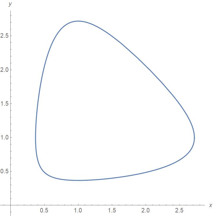
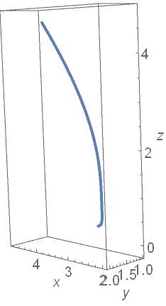
Figure 2. Left: a multiplicative circle at centered $(1,1)$ and radius $e$. Right: a multiplicative rectifying curve parametrized by Eq. (1), $0.5\leq t\leq 3$.

More clearly, consider the following subset of $\mathbb{R}^{2}$ (see Figure 2)

$$C=\{(x,y)\in\mathbb{R}^{2}:(\log x)^{2}+(\log y)^{2}=1,x,y>0\}.$$

We also can parameterize this set as $x(t)=e^{\cos(\log t)}$ and $y(t)=e^{\sin(\log t)}$, $t>0$. If we use the usual arithmetic operations, derivative and integral, then it would not be easy to understand what the set $C$ expresses geometrically. With or without the help of computer programs, we cannot even calculate its basic invariants, e.g., the arc length function $s(t)$ is given by a complicated integral

$$s(t)=\int^{t}\frac{1}{u}\left((\sin(\log u)e^{\cos(\log u)})^{2}+(\cos(\log u)e^{\sin(\log u)})^{2}\right)^{1/2}du.$$

However, applying the multiplicative tools, we see that $C$ is indeed a multiplicative circle parameterized by the multiplicative arc length whose center is $(1,1)$ and radius $e$, which is one of the simplest multiplicative curves (see Section 3). This is the reason why, in some cases, the multiplicative tools need to be applied instead of the usual ones.

In the case of the dimension $3$, the determination of geometric objects sometimes becomes more difficult when the multiplicative tools are omitted. For example, consider the following parameterized curve (see Fig. 2)

(1) $$x(t)=e^{\sec(\log t)/\sqrt{2}},\quad y(t)=e^{\sec(\log t)\cos(\log t^{\sqrt{2}})/\sqrt{2}},\quad z(t)=e^{\sec(\log t)\sin(\log t^{\sqrt{2}})/\sqrt{2}},t>0.$$

As in the case of the multiplicative circle, it would not be easy to work geometrically on this curve by the means of the usual differential geometry. However, from the perspective of multiplicative differential geometry, it is a multiplicative rectifying curve, a type of parameterized space curves introduced by B.-Y. Chen [14] in 2003.

On the other hand, if one uses the multiplicative derivative together with the usual arithmetic operations, then one would have some difficulties; for example, it would not satisfy the properties such as linearity, chain rule, Leibniz rule and so on (see [8]). However, these are essential tools to establish a differential-geometric theory. To overcome these difficulties, Svetlin [22] proposed a useful idea, which is explained as follows.

Let $\mathbb{R}^{n}$ be the real vector space of the dimension $n\geq 2$. A multiplicative Euclidean space $\mathbb{E}^{n}_{*}$ is the pair $(\mathbb{R}^{n},\langle,\rangle_{*})$ where $\langle,\rangle_{*}$ is the so-called multiplicative Euclidean inner product. We note that the usual vector addition and scalar multiplication on $\mathbb{R}^{n}$ are now replaced with the multiplicative operations (see Section 2). With these new arithmetic operations, the multiplicative derivative has the properties that a derivative has. Therefore, it is now suitable for our purpose.

We would like to emphasize the importance of the rectifying curves whose position vector always lies in its own rectifying plane, because of their close relationship to spherical curves, helices, geodesics and centrodes in mechanics, see [15, 16, 19]. In addition, we point out the underlying space of $\mathbb{E}_{*}^{3}$ is $\mathbb{R}^{3}$ and the definition of rectifying curve is affine and not metric. Hence, if we want to examine the geometric features of the rectifying curves, we may directly use the multiplicative differential-geometric concepts. These are the justifications that we consider such curves in $\mathbb{E}^{3}_{*}$.

The structure of the paper is as follows. After some preliminaries on multiplicative algebra and calculus (Section 2), we will recall in Section 3 the curvatures and Frenet formulas of multiplicative space curves. In Proposition 3.3, we will characterize multiplicative curves lying on a multiplicative sphere in terms of their curvatures. In Section 4, we will introduce the multiplicative counterpart to the notion of rectifying curves. We will completely classify multiplicative rectifying curves using multiplicative spherical curves (Theorem 4.5). Before that, however, we will need to prove some results characterizing rectifying curves in terms of their curvatures and the multiplicative distance function (Propositions 4.1, 4.2, 4.3, 4.4).

2. Preliminaries

In the present section we recall the multiplicative arguments from algebra and calculus, cf. [22, 23, 24].

Let $\mathbb{R}_{*}$ be the set of all the positive real numbers. For $a,b\in\mathbb{R}_{*}$ we set

$$a+_{*}b = e^{\log a+\log b},$$

$$a-_{*}b = e^{\log a-\log b},$$

$$a\cdot_{*}b = e^{\log a\cdot\log b},$$

$$a/_{*}b = e^{\log a/\log b},\quad b\neq 1.$$

Here, for some $a\in\mathbb{R}_{*}$, we also have

$$a^{2_{*}}=e^{(\log a)^{2}},\quad a^{\frac{1}{2}_{*}}=e^{\sqrt{\log a}}.$$

It is direct to conclude that the triple $(\mathbb{R}_{*},+_{*},\cdot_{*})$ is a field. We denote by $\mathbb{R}_{*}$ this field for convenience. Introduce

$$\left|a\right|_{*}=\left\{\begin{array}[]{ll}a,&a\in[1,\infty)\\ 1/a,&a\in(0,1).\end{array}\right.$$

Given $x\mapsto f(x)\in\mathbb{R}_{*}$, $x\in I\subset\mathbb{R}_{*}$, the multiplicative derivative of $f$ at $x$ is defined by

$$f^{*}(x)=\lim_{h\rightarrow 1}(f(x+_{*}h)-_{*}f(x))/_{*}h.$$

In terms of the usual arithmetical operations,

$$f^{*}(x)=\lim_{h\rightarrow 1}\left(\frac{f(hx)}{f(x)}\right)^{1/\log h},$$

or by L’ Hospital’s rule,

$$f^{*}(x)=e^{x(\log f(x))^{\prime}},$$

where the prime is the usual derivative with respect to $x$.

Denote by $f^{*(n)}(x)$ the $n$th-order multiplicative derivative of $f(x)$ which is the multiplicative derivative of $f^{*(n-1)}(x)$, for some positive integer $n>1$. We call the function $f(x)$ multiplicative differentiable on $I$ if $f^{*(n)}(x)$ exists where, if necessary, $n$ may be extended in maximum order that will be needed.

We may easily conclude that the multiplicative derivative holds some essential properties as linearity, Leibniz rule and chain rules (see [23]).

The multiplicative integral of the function $f(x)$ in an interval $[a,b]\subset\mathbb{R}_{*}$ is defined by

$$\int_{*a}^{b}f(x)\cdot_{*}{d_{*}x}=e^{\int_{a}^{b}\frac{1}{x}\log f(x)dx}.$$

Let $\mathbb{R}_{*}^{n}=\{(x_{1},...,x_{n}):x_{1},...,x_{n}\in\mathbb{R}_{*}\}$ and $\mathbf{x},\mathbf{y}\in\mathbb{R}_{*}^{n}$. Then $\mathbb{R}_{*}^{n}$ is a vector space on $\mathbb{R}_{*}$ with the pair of operations

$$\mathbf{x}+_{*}\mathbf{y} = (x_{1}+_{*}y_{1},...,x_{n}+_{*}y_{n})=(x_{1}y_{1},...,x_{n}y_{n}),$$

$$a\cdot_{*}\mathbf{x} = (a\cdot_{*}x_{1},...,a\cdot_{*}y_{n})=(e^{\log a\log x_{1}},...,e^{\log a\log x_{n}}),\quad a\in\mathbb{R}_{*}.$$

The elements of multiplicative canonical basis of $\mathbb{R}_{*}^{n}$ are

$$\mathbf{e}_{1}=(1_{*},0_{*}...,0_{*}),\mathbf{e}_{2}=(0_{*},1_{*},...,0_{*}),...,\mathbf{e}_{n}=(0_{*},0_{*},...,1_{*}),$$

where $0_{*}=1$ and $1_{*}=e$. Also, denote by $\mathbf{0}_{*}=(0_{*},...,0_{*})$ the multiplicative zero vector.

A positive-definite scalar product on $\mathbb{R}_{*}^{n}$ is defined by

$$\langle\mathbf{x},\mathbf{y}\rangle_{*}=x_{1}\cdot_{*}y_{1}+_{*}...+_{*}x_{n}\cdot_{*}y_{n}=e^{\log x_{1}\log y_{1}+...+\log x_{n}\log y_{n}}.$$

We call $\langle,\rangle_{*}$ multiplicative Euclidean inner product and $(\mathbb{R}_{*}^{n},\langle,\rangle_{*})$ multiplicative Euclidean space denoted by $\mathbb{E}_{*}^{n}$. Also, we call two vectors $\mathbf{x}$ and $\mathbf{y}$ multiplicative orthogonal if $\langle\mathbf{x},\mathbf{y}\rangle_{*}=0_{*}$. The induced multiplicative Euclidean norm $\|\cdot\|_{*}$ on $\mathbb{E}_{*}^{n}$ is

$$\|\mathbf{x}\|_{*}=(\langle\mathbf{x},\mathbf{y}\rangle_{*})^{\frac{1}{2}_{*}}=e^{\sqrt{\log x_{1}^{2}+...+\log x_{n}^{2}}}.$$

A vector $\mathbf{x}$ with $\|\mathbf{x}\|_{*}=1_{*}$ is said to be multiplicative unitary.

Let $\theta\in[0_{*},e^{\pi}]$. We then introduce

$$\cos_{*}\theta=e^{\cos(\log\theta)},\quad\arccos_{*}\phi=e^{\arccos(\log\phi)},$$

for $\phi\in[e^{-1},1_{*}]$. Then, the multiplicative radian measure of multiplicative angle between $\mathbf{x}$ and $\mathbf{y}$ is defined by

$$\theta=\arccos_{*}\left(\langle\mathbf{x},\mathbf{y}\rangle_{*}/_{*}(\|\mathbf{x}\|_{*}\cdot_{*}\|\mathbf{y}\|_{*})\right)=\arccos_{*}\left(e^{\frac{\log\langle\mathbf{x},\mathbf{y}\rangle_{*}}{\log\|\mathbf{x}\|_{*}\log\|\mathbf{y}\|_{*}}}\right).$$

The multiplicative cross product of $\mathbf{x}$ and $\mathbf{y}$ in $\mathbb{E}_{*}^{3}$ is defined by

$$\mathbf{x}\times_{*}\mathbf{y}=(e^{\log x_{2}\log y_{3}-\log x_{3}\log y_{2}},e^{\log x_{3}\log y_{1}-\log x_{1}\log y_{3}},e^{\log x_{1}\log y_{2}-\log x_{2}\log y_{1}}).$$

It is direct to prove that the multiplicative cross product holds the standart algebraic and geometric properties. For example, $\mathbf{x}\times_{*}\mathbf{y}$ is multiplicative orthogonal to $\mathbf{x}$ and $\mathbf{y}$. In addition, $\mathbf{x}\times_{*}\mathbf{y}=\mathbf{0}_{*}$ if and only if $\mathbf{x}$ and $\mathbf{y}$ are multiplicative collinear.

A multiplicative line passing through a point $P=(p_{1},p_{2},p_{3})$ and multiplicative parallel to $\mathbf{v}=(v_{1},v_{2},v_{3})$ is a subset of $\mathbb{E}_{*}^{3}$ defined by

$$\{Q=(q_{1},q_{2},q_{3})\in\mathbb{E}_{*}^{3}:Q=P+_{*}t\cdot_{*}\mathbf{v}\},$$

where $q_{i}=e^{\log p_{i}+\log t\log v_{i}}$, $i=1,2,3$. We point out that the multiplicative parallelism is algebraically equivalent to multiplicative collinearity.

A multiplicative plane passing through a point $P$ and multiplicative orthogonal to $\mathbf{v}$ is a subset of $\mathbb{E}_{*}^{3}$ defined by

$$\{Q\in\mathbb{E}_{*}^{3}:\langle Q-_{*}P,\mathbf{v}\rangle_{*}=0_{*}\},$$

where

$$e^{(\log q_{1}-\log p_{1})\log v_{1}+(\log q_{2}-\log p_{2})\log v_{2}+(\log q_{3}-\log p_{3})\log v_{3}}=0_{*}.$$

A multiplicative sphere with radius $r>0_{*}$ and centered at $C=(c_{1},c_{2},c_{3})\in\mathbb{E}_{*}^{3}$ is a subset of $\mathbb{E}_{*}^{3}$ defined by

$$\{Q\in\mathbb{E}_{*}^{3}:\|Q-_{*}C\|_{*}=r\},$$

where

$$e^{(\log q_{1}-\log c_{1})^{2}+(\log q_{2}-\log c_{2})^{2}+(\log q_{3}-\log c_{3})^{2}}=e^{(\log r)^{2}}.$$

3. Differential geometry of curves in $\mathbb{E}_{*}^{3}$

Consider a function $\mathbf{x}:I\subset\mathbb{R}_{*}\to\mathbb{E}_{*}^{3}$ where $s\mapsto\mathbf{x}(s)=(x_{1}(s),x_{2}(s),x_{3}(s))$. Suppose that $x_{i}(s)$ ($i=1,2,3$) is multiplicative differentiable on $I$, setting $\mathbf{x}^{*}(s)=(x^{*}_{1}(s),x_{2}^{*}(s),x_{3}^{*}(s)).$

We call the subset $\mathcal{C}\subset\mathbb{E}_{*}^{3}$ which is the range of $\mathbf{x}(s)$ a multiplicative curve. Here $\mathbf{x}(s)$ is said to be a multiplicative parametrization of $\mathcal{C}$. We also call $\mathbf{x}(s)$ a multiplicative regular parameterized curve if nowhere $\mathbf{x}^{*}(s)$ is $\mathbf{0}_{*}$. If, also, $\|\mathbf{x}^{*}(s)\|_{*}=1_{*}$, or equivalently,

$$e^{(\log x_{1}^{*})^{2}+(\log x_{2}^{*})^{2}+(\log x_{3}^{*})^{2}}=1_{*},\quad\text{ for every }s\in I,$$

then we call that $\mathcal{C}$ is parametrized by multiplicative arc length.

We may easily observe that a multiplicative arc length parameter is independent from the multiplicative translations. In addition, one always could find a multiplicative arc length parameter of the curve $\mathcal{C}$ (see [22]). In the remaining part, unless otherwise specified, we will assume that $\mathbf{x}(s)$ in $\mathbb{E}_{*}^{3}$ is a multiplicative arc length parameterized curve.

We call that $\mathbf{u}(t)=(u_{1}(t),...,u_{n}(t))$ is a multiplicative differentiable vector field along the curve $\mathcal{C}$ if each $u_{i}(t)$ is multiplicative differentiable on $I$, $i=1,...,n$. If $\mathbf{u}(t)$ and $\mathbf{v}(t)$ are two multiplicative differentiable vector fields on $\mathcal{C}$, then it is direct to conclude

(2) $$(\langle\mathbf{u}(t),\mathbf{v}(t)\rangle_{*})^{*}=\langle\mathbf{u}^{*}(t),\mathbf{v}(t)\rangle_{*}+_{*}\langle\mathbf{u}(t),\mathbf{v}^{*}(t)\rangle_{*}.$$

Assume that $\mathbf{x}(s)$ is multiplicative biregular, that is, nowhere $\mathbf{x}^{*}(s)$ and $\mathbf{x}^{**}(s)$ are multiplicative collinear. We consider a trihedron $\{\mathbf{t}(s),\mathbf{n}(s),\mathbf{b}(s)\}$ along $\mathbf{x}(s)$, so-called multiplicative Frenet frame, where

$$\left.\begin{array}[]{l}\mathbf{t}(s)=\mathbf{x}^{*}(s),\\ \mathbf{n}(s)=\mathbf{x}^{**}(s)/_{*}\|\mathbf{x}^{**}(s)\|_{*},\\ \mathbf{b}(s)=\mathbf{t}(s)\times_{*}\mathbf{n}(s).\end{array}\right.$$

Hence, by setting $\mathbf{t}(s)=(t_{1}(s),t_{2}(s),t_{3}(s))$, $\mathbf{n}(s)=(n_{1}(s),n_{2}(s),n_{3}(s))$ and $\mathbf{b}(s)=(b_{1}(s),b_{2}(s),b_{3}(s))$, we have

$$\left.\begin{array}[]{l}t_{i}=x_{i}^{*},\\ n_{i}=e^{\frac{\log x_{i}^{**}}{\sqrt{(\log x_{1}^{**})^{2}+(\log x_{2}^{**})^{2}+(\log x_{3}^{**})^{2}}}},\\ b_{i}=e^{(-1)^{j+k-1}(\log t_{j}\log n_{k}-\log t_{k}\log n_{j})},i,j,k\in\{1,2,3\},\end{array}\right.$$

where $j\neq i\neq k$ and $j<k$.

The vector field $\mathbf{t}(s)$ (resp. $\mathbf{n}(s)$ and $\mathbf{b}(s)$) along $\mathbf{x}(s)$ is said to be multiplicative tangent (resp. principal normal and binormal). It is direct to prove that $\{\mathbf{t}(s),\mathbf{n}(s),\mathbf{b}(s)\}$ is mutually multiplicative orthogonal and $\mathbf{n}(s)\times_{*}\mathbf{b}(s)=\mathbf{t}(s)$ and $\mathbf{b}(s)\times_{*}\mathbf{t}(s)=\mathbf{n}(s)$. We also point out that the arc length parameter and multiplicative Frenet frame are independent from the choice of multiplicative parametrization [22].

We define the multiplicative curvature $\kappa(s)$ and torsion $\tau(s)$ as

$$\kappa(s)=\|\mathbf{x}^{**}(s)\|_{*}=e^{\sqrt{(\log(x_{1}^{**}(s))^{2}+(\log(x_{2}^{**}(s))^{2}+(\log(x_{3}^{**}(s))^{2}}}$$

and

$$\tau(s)=\langle\mathbf{n}^{*}(s),\mathbf{b}(s)\rangle_{*}=e^{\log n_{1}^{*}(s)\log b_{1}(s)+\log n_{2}^{*}(s)\log b_{2}(s)+\log n_{3}^{*}(s)\log b_{3}(s)}.$$

The multiplicative Frenet formulas are now

$$\left.\begin{array}[]{l}\mathbf{t}^{*}=\kappa\cdot_{*}\mathbf{n},\\ \mathbf{n}^{*}=-_{*}\kappa\cdot_{*}\mathbf{t}+_{*}\tau\cdot_{*}\mathbf{b}\\ \mathbf{b}^{*}=-_{*}\tau\cdot_{*}\mathbf{n},\\ \end{array}\right.$$

or equivalently,

$$\left.\begin{array}[]{l}t_{i}^{*}=e^{\log\kappa\log n_{i}},\\ n_{i}^{*}=e^{-\log\kappa\log t_{i}+\log\tau\log b_{i}},\\ b_{i}^{*}=e^{-\log\tau\log n_{i}},\quad i=1,2,3.\\ \end{array}\right.$$

We call $\mathbf{x}(s)$ multiplicative twisted if nowhere $\kappa(s)$ and $\tau(s)$ is $0_{*}$. The multiplicative analogous of the fundamental theorem for space curves is the following (see [22, p. 132-135]).

Theorem 3.1 (Existence).

[22] Given multiplicative differentiable functions $f(s)>0_{*}$, $g(s)$ on $I$. Then, there is a unique multiplicative parametrized curve whose $\kappa(s)=f(s)$ and $\tau(s)=g(s)$.

Theorem 3.2 (Uniqueness).

[22] Given two multiplicative parametrized curves $\mathbf{x}(s)$ and $\mathbf{y}(s)$, $s\in I$, whose $\kappa_{\mathbf{x}}(s)=\kappa_{\mathbf{y}}(s)$ and $\tau_{\mathbf{x}}(s)=\tau_{\mathbf{y}}(s)$. Then, there is a multiplicative rigid motion $F$ such that $\mathbf{y}(s)=F(\mathbf{x}(s))$.

The multiplicative osculating (resp. normal and rectifying) plane of $\mathbf{x}(s)$ at some $s\in I$ is a multiplicative plane passing through $\mathbf{x}(s)$ and multiplicative orthogonal to $\mathbf{b}(s)$ (resp. $\mathbf{t}(s)$ and $\mathbf{n}(s)$).

We notice that $\mathbf{x}(s)$ is a subset of a multiplicative line if and only if $\kappa(s)$ is $0_{*}$ on $I$. Analogously, $\mathbf{x}(s)$ is a subset of multiplicative osculating plane itself if and only if $\tau(s)$ is $0_{*}$ on $I$. We call $\mathbf{x}(s)$ is a multiplicative spherical curve if it is a subset of a multiplicative sphere.

In terms of the multiplicative Frenet frame, we can write the decomposition for $\mathbf{x}(s)$ as

(3) $$\mathbf{x}(s)=\langle\mathbf{x}(s),\mathbf{t}(s)\rangle_{*}\cdot_{*}\mathbf{t}(s)+_{*}\langle\mathbf{x}(s),\mathbf{n}(s)\rangle_{*}\cdot_{*}\mathbf{n}(s)+_{*}\langle\mathbf{x}(s),\mathbf{b}(s)\rangle_{*}\cdot_{*}\mathbf{b}(s),$$

or equivalently,

(4) $$x_{i}(s)=e^{\log\langle\mathbf{x}(s),\mathbf{t}(s)\rangle_{*}\log t_{i}+\log\langle\mathbf{x}(s),\mathbf{n}(s)\rangle_{*}\log n_{i}+\log\langle\mathbf{x}(s),\mathbf{b}(s)\rangle_{*}\log b_{i}},\quad i=1,2,3.$$

Here we call the functions $\langle\mathbf{x}(s),\mathbf{t}(s)\rangle_{*}$, $\langle\mathbf{x}(s),\mathbf{n}(s)\rangle_{*}$ and $\langle\mathbf{x}(s),\mathbf{b}(s)\rangle_{*}$ the multiplicative tangential, principal normal and binormal components of $\mathbf{x}(s)$, respectively. In addition, denote by $\mathbf{x}^{\intercal_{*}}$ the multiplicative tangential component and by $\mathbf{x}^{\perp_{*}}$ multiplicative normal component. Then,

$$\|\mathbf{x}^{\intercal_{*}}(s)\|_{*}=\langle\mathbf{x}(s),\mathbf{t}(s)\rangle_{*}=e^{\log x_{1}\log t_{1}+\log x_{2}\log t_{2}+\log x_{3}\log t_{3}},$$

and

$$\left.\begin{array}[]{l}\|\mathbf{x}^{\perp_{*}}(s)\|_{*}=e^{\sqrt{(\log\langle\mathbf{x}(s),\mathbf{n}(s)\rangle_{*})^{2}+(\log\langle\mathbf{x}(s),\mathbf{b}(s)\rangle_{*})^{2}}}\\ =e^{\sqrt{(\log x_{1}\log n_{1}+\log x_{2}\log n_{2}+\log x_{3}\log n_{3})^{2}+(\log x_{1}\log b_{1}+\log x_{2}\log b_{2}+\log x_{3}\log b_{3})^{2}}}.\end{array}\right.$$

Next, we give a characterization of the multiplicative spherical curves with $\kappa,\tau\neq 0_{*}$ in terms of their multiplicative position vectors. Without loss of generality, we will assume that $\mathbb{S}_{*}^{2}$ is a multiplicative sphere with radius $r>0_{*}$ and centered at $\mathbf{0}_{*}$.

Proposition 3.3.

Let $\mathbf{x}(s)\subset\mathbb{E}_{*}^{3}$ be a multiplicative twisted curve. If $\mathbf{x}(s)\subset\mathbb{S}_{*}^{2}$, then

$$\mathbf{x}(s)=(e^{-1}/_{*}\kappa(s))\cdot_{*}\mathbf{n}(s)+_{*}((e^{-1}/_{*}\kappa(s))^{*}/_{*}\tau(s))\cdot_{*}\mathbf{b}(s)$$

or equivalently

$$x_{i}(s)=e^{-\log n_{i}(s)/\log\kappa(s)+(-1/\log\kappa(s))^{*}\log b_{i}(s)/\log\tau(s)}.$$

Proof.

By the assumption, because $\mathbf{x}(s)\subset\mathbb{S}_{*}^{2}$, we have $\|\mathbf{x}(s)\|_{*}=r$, for every $s$. It is equivalent to

(5) $$\langle\mathbf{x}(s),\mathbf{x}(s)\rangle_{*}=e^{(\log r)^{2}}.$$

If we take multiplicative differentiation of both-hand sides in Eq. (5) with respect to $s$ then we have

$$(\langle\mathbf{x}(s),\mathbf{x}(s)\rangle_{*})^{*}=\left(e^{(\log r)^{2}}\right)^{*},$$

or, by Eq. (2),

(6) $$e^{2}\cdot_{*}\langle\mathbf{x}(s),\mathbf{x}^{*}(s)\rangle_{*}=0_{*}.$$

We understand from Eq. (6) that the multiplicative tangential component of $\mathbf{x}(s)$ is

(7) $$\langle\mathbf{x}(s),\mathbf{t}(s)\rangle_{*}=0_{*}.$$

Again we take multiplicative differentiation of both-hand sides in Eq. (7) with respect to $s$, and we have

$$(\langle\mathbf{x}(s),\mathbf{t}(s)\rangle_{*})^{*}=(0_{*})^{*},$$

or

$$\langle\mathbf{t}(s),\mathbf{t}(s)\rangle_{*}+_{*}\langle\mathbf{x}(s),\mathbf{t}^{*}(s)\rangle_{*}=0_{*}.$$

Using the multiplicative Frenet formulas,

$$1_{*}+_{*}\kappa(s)\cdot_{*}\langle\mathbf{x}(s),\mathbf{n}^{*}(s)\rangle_{*}=0_{*}$$

or

(8) $$\langle\mathbf{x}(s),\mathbf{n}(s)\rangle_{*}=e^{-1}/_{*}\kappa(s).$$

If we apply the same arguments in Eq. (8) and consider Eq. (7), then we obtain

(9) $$\langle\mathbf{x}(s),\mathbf{b}(s)\rangle_{*}=(e^{-1}/_{*}\kappa(s))^{*}/_{*}\tau(s).$$

The result of the theorem follows by replacing Eqs. (7), (8), (9) in Eqs. (3) and (4), respectively. ∎

As a direct conseqeunce of Proposition 3.3, if $\mathbf{x}(s)$ is multiplicative twisted and if $\mathbf{x}(s)\subset\mathbb{S}_{*}^{2}$, then

$$r=\left((e^{-1}/_{*}\kappa(s))^{2_{*}}+_{*}((e^{-1}/_{*}\kappa(s))^{*}/_{*}\tau(s)))^{2_{*}})\right)^{\frac{1}{2}_{*}}$$

or equivalently,

$$(\log r)^{2}=\left(\frac{1}{\log\kappa(s)}\right)^{2}+\left(\frac{e^{s(-1/\log\kappa(s))^{\prime}}}{\log\tau(s)}\right)^{2},$$

where the prime ^′ denotes the usual derivative with respect to $s$.

We point out that Proposition 3.3 is valid for a multiplicative twisted curve. However, even in the case $\tau(s)=0_{*}$, we may use the arguments given in its proof. More explicitly, assume that $\mathbf{x}(s)\subset\mathbb{S}_{*}^{2}$ with $\tau(s)=0_{*}$. Then, if we take multiplicative differentiation in Eq. (8), we derive that $\langle\mathbf{x}(s),\mathbf{b}(s)\rangle_{*}=0_{*}$, implying that $\mathbf{x}(s)$ and $\mathbf{n}(s)$ are multiplicative collinear due to Eq. (7). Hence, we conclude that $\mathbf{x}(s)=(e^{-1}/_{*}\kappa(s))\cdot_{*}\mathbf{n}(s)$ and $r=|e^{-1}/_{*}\kappa(s)|_{*}$, or equivalently,

$$x_{i}(s)=e^{(-1/\log\kappa(s))\log n_{i}(s)}\quad\text{and}\quad r=|e^{-1/\log\kappa(s)}|_{*},\quad i=1,2,3.$$

As an example, we may take such a multiplicative spherical curve of $\mathbb{S}_{*}^{2}$ with radius $1_{*}$, called multiplicative great circle, as follows. Let $\Gamma$ pass through $\mathbf{0}_{*}$ and multiplicative orthogonal to $\mathbf{e}_{3}$. Consider the multiplicative equator (see Fig. 1)

$$\mathcal{C}=\Gamma\cap\mathbb{S}_{*}^{2}=\{(x,y,z)\in\mathbb{E}_{*}^{3}:(\log x)^{2}+(\log y)^{2}=1,z=1\}.$$

It can be parametrized by its multiplicative arclength as $\mathbf{x}(s)=\left(e^{\cos\log s},e^{\sin\log s},1\right)$. Here, by a direct calculation, we may observe that

$$\kappa(s)=1_{*}\quad\text{and}\quad\mathbf{n}(s)=\left(e^{-\cos\log s},e^{-\sin\log s},1\right),$$

implying $\mathbf{x}(s)=e^{-1}\cdot_{*}\mathbf{n}(s)$.

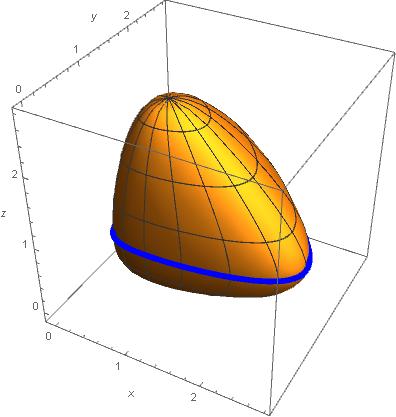
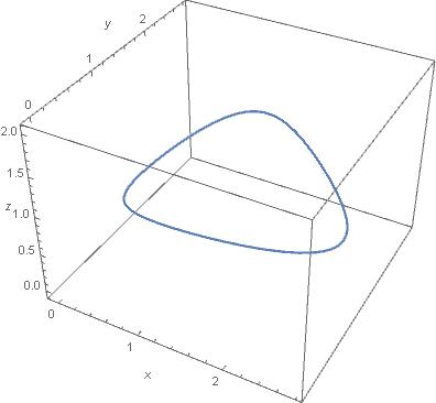
Figure 1. A multiplicative equator of $\mathbb{S}_{*}^{2}$

4. Multiplicative rectifying curves

In this section we will introduce the multiplicative analogous of the rectifying curves and then present some characterization and classification results.

Given a multiplicative biregular curve $\mathbf{x}(s)$ in $\mathbb{E}_{*}^{3}$, $s\in I\subset\mathbb{R}_{*}$, where $\{\mathbf{t}(s),\mathbf{n}(s),\mathbf{b}(s)\}$ is the multiplicative Frenet frame. We call $\mathbf{x}(s)$ a multiplicative rectifying curve if the multiplicative principal normal component is $0_{*}$. In other words, $\langle\mathbf{x}(s),\mathbf{n}(s)\rangle_{*}=0_{*},$ for every $s\in I$ and so Eq. (3) is now

(10) $$\mathbf{x}(s)=\lambda(s)\cdot_{*}\mathbf{t}(s)+_{*}\mu(s)\cdot_{*}\mathbf{b}(s),$$

where $\lambda(s)=\langle\mathbf{x}(s),\mathbf{t}(s)\rangle_{*}$ and $\mu(s)=\langle\mathbf{x}(s),\mathbf{b}(s)\rangle_{*}$. In terms of the usual operations, Eq. (10) writes as

$$x_{i}(s)=e^{\log\lambda(s)\log t_{i}(s)+\log\mu(s)\log b_{i}(s)},\quad i=1,2,3.$$

The first result of this section characterizes the multiplicative rectifying curves in terms of their multiplicative tangent and binormal components.

Proposition 4.1.

If $\mathbf{x}(s)\subset\mathbb{E}_{*}^{3}$ with $\kappa\neq 0_{*}$ is a multiplicative rectifying curve, then nowhere the multiplicative torsion is $0_{*}$ and

$$\langle\mathbf{x}(s),\mathbf{t}(s)\rangle_{*}=s+_{*}a=as,\quad\langle\mathbf{x}(s),\mathbf{b}(s)\rangle_{*}=b,\quad a,b\in\mathbb{R}_{*},b\neq 0_{*}.$$

The converse statement is true as well.

Proof.

Assume that $\mathbf{x}(s)$ is a multiplicative rectifying curve. Taking a multiplicative differentiation in Eq. (10),

$$\mathbf{x}^{*}(s)=\lambda^{*}(s)\cdot_{*}\mathbf{t}(s)+_{*}\lambda(s)\cdot_{*}\mathbf{t}^{*}(s)+_{*}\mu^{*}(s)\cdot_{*}\mathbf{b}(s)+_{*}\mu(s)\cdot_{*}\mathbf{b}^{*}(s).$$

The multiplicative Frenet formulas follow

$$(\lambda^{*}(s)-_{*}1_{*})\cdot_{*}\mathbf{t}(s)+_{*}(\lambda^{*}(s)\cdot_{*}\kappa(s)-_{*}\mu(s)\cdot_{*}\tau(s))\cdot_{*}\mathbf{n}(s)+\mu^{*}(s)\cdot_{*}\mathbf{b}(s)=\mathbf{0}_{*}.$$

Due to the multiplicative linearly independence,

(11) $$\lambda^{*}(s)=1_{*},\quad\lambda(s)\cdot_{*}\kappa(s)=\mu(s)\cdot_{*}\tau(s),\quad\mu^{*}(s)=0_{*}.$$

We here conclude that

$$\lambda(s)=\int_{*}^{s}1_{*}\cdot_{*}{d_{*}u}=e^{\int^{s}\frac{1}{u}\log edu}=e^{\log s+\log a}=s+_{*}a,\quad a>0,$$

and

$$\mu(s)=\int_{*}^{s}0_{*}\cdot_{*}{d_{*}u}=e^{\int^{s}\frac{1}{u}\log 1du}=e^{\log b}=b,\quad b>0.$$

Notice here that $b\neq 0_{*}$ because otherwise one derives from the middle equation in Eq. (11) that $\kappa(s)$ is $0_{*}$. This contradicts with biregularity of $\mathbf{x}(s)$. Analogously, $\tau(s)$ is nowhere $0_{*}$.

Conversely, suppose that the multiplicative tangential and binormal components are

$$\langle\mathbf{x}(s),\mathbf{t}(s)\rangle_{*}=s+_{*}a,\quad\langle\mathbf{x}(s),\mathbf{b}(s)\rangle_{*}=b,$$

where $a,b\in\mathbb{R}_{*},b\neq 0_{*}$. Using Eq. (2),

$$0_{*} = (\langle\mathbf{x}(s),\mathbf{b}(s)\rangle_{*})^{*}$$

$$= \langle\mathbf{x}^{*}(s),\mathbf{b}(s)\rangle_{*}+_{*}\langle\mathbf{x}(s),\mathbf{b}^{*}(s)\rangle_{*}$$

$$= \langle\mathbf{t}(s),\mathbf{b}(s)\rangle_{*}-_{*}\tau(s)\langle\mathbf{x}(s),\mathbf{n}(s)\rangle_{*}$$

$$= -_{*}\tau(s)\langle\mathbf{x}(s),\mathbf{n}(s)\rangle_{*}.$$

Since the multiplicative curvatures are nowhere $0_{*}$, we may easily obtain $\langle\mathbf{x}(s),\mathbf{n}(s)\rangle_{*}=0_{*}$. This completes the proof. ∎

Besides Proposition 4.1, several characterizations of multiplicative rectifying curves may be presented as follows.

Proposition 4.2.

If $\mathbf{x}(s)\subset\mathbb{E}_{*}^{3}$ is a multiplicative rectifying curve, then the multiplicative ratio of the multiplicative curvatures is

$$\tau(s)/_{*}\kappa(s)=c\cdot_{*}s+_{*}d=e^{c\log s+\log d},\quad c,d\in\mathbb{R}_{*},c\neq 0_{*}.$$

The converse statement is true as well.

Proof.

By the middle equation in Eq. (11), one writes

$$\tau(s)/_{*}\kappa(s)=\lambda(s)/_{*}\mu(s)=(s+_{*}a)/_{*}b=e^{\frac{\log s+\log a}{\log b}},\quad a,b\in\mathbb{R}_{*},b\neq 0_{*}.$$

Setting $\log c=1/\log b$ and $\log d=\log a/\log b$ gives the first part of the proof.

Conversely, suppose that $\mathbf{x}(s)$ with $\kappa\neq 0_{*}$ holds $\tau(s)/_{*}\kappa(s)=c\cdot_{*}s+_{*}d$, for $c,d\in\mathbb{R}_{*},c\neq 0_{*}.$ Also, we may write

$$\tau(s)/_{*}\kappa(s)=(s+_{*}a)/_{*}b,\quad a,b\in\mathbb{R}_{*},b\neq 0_{*}$$

or equivalently,

$$b\cdot_{*}\tau(s)-_{*}(s+_{*}a)\cdot_{*}\kappa(s)=0_{*}.$$

We now set

$$f(s)=\mathbf{x}(s)-_{*}(s+_{*}a)\cdot_{*}\mathbf{t}(s)-_{*}b\cdot_{*}\mathbf{b}(s),$$

where $f(s)$ is multiplicative differentiable on its domain. If we take multiplicative differentiation of the last equation and if we use the multiplicative Frenet formulas, then we obtain

$$f^{*}(s)=[-_{*}(s+_{*}a)\cdot_{*}\kappa(s)+_{*}b\cdot_{*}\tau(s)]\cdot_{*}\mathbf{n}(s).$$

Here concludes that $f^{*}(s)=0_{*}$ or equivalently $f(s)$ is constant. Then, $\mathbf{x}(s)$ is multiplicative congruent to a multiplicative rectifying curve. ∎

We define the multiplicative distance function of $\mathbf{x}(s)$ as $\rho(s)=\|\mathbf{x}(s)\|_{*}$. Hence, we have the following.

Proposition 4.3.

If $\mathbf{x}(s)\subset\mathbb{E}_{*}^{3}$ is a multiplicative rectifying curve with $\kappa>0_{*}$, then

(12) $$\rho(s)^{2_{*}}=s^{2_{*}}+_{*}e^{c}\cdot_{*}s+_{*}e^{d},\quad c,d\in\mathbb{R},d>0,$$

or equivalently,

$$e^{(\log\rho(s))^{2}}=e^{(\log s)^{2}+c\log s+d}.$$

The converse statement is true as well.

Proof.

Assume that $\mathbf{x}(s)$ is a multiplicative rectifying curve. It then follows from Eq. (10) that

$$\rho(s)^{2_{*}}=\langle\mathbf{x}(s),\mathbf{x}(s)\rangle_{*}=\lambda(s)^{2_{*}}+_{*}\mu(s)^{2_{*}}.$$

Here, by Proposition 4.1 we know that $\lambda(s)=s+_{*}a$ and $\mu(s)=b$, for $a,b\in\mathbb{R}_{*}$, $b\neq 0_{*}$. Hence

$$\rho(s)^{2_{*}}=s^{2_{*}}+_{*}e^{2}\cdot_{*}a\cdot_{*}s+_{*}a^{2_{*}}+_{*}b^{2_{*}}.$$

Setting

$$e^{c}=e^{2}\cdot_{*}a=e^{2\log a},\quad e^{d}=a^{2_{*}}+_{*}b^{2_{*}}=e^{(\log a)^{2}+(\log b)^{2}},$$

we arrive to Eq. (12). Conversely, let Eq. (12) hold. We will show that $\mathbf{x}(s)$ is a multiplicative rectifying curve. Then,

$$\langle\mathbf{x}(s),\mathbf{x}(s)\rangle_{*}=s^{2_{*}}+_{*}e^{c}\cdot_{*}s+_{*}e^{d}.$$

Taking multiplicative differentiation, we have

$$e^{2}\cdot_{*}\langle\mathbf{t}(s),\mathbf{x}(s)\rangle_{*}=e^{2}\cdot_{*}s+_{*}c,$$

or, because $e^{c}/_{*}e^{2}=a$,

$$\langle\mathbf{t}(s),\mathbf{x}(s)\rangle_{*}=s+_{*}a.$$

We again take multiplicative differentiation, obtaining

$$1_{*}+_{*}\kappa(s)\cdot_{*}\langle\mathbf{n}(s),\mathbf{x}(s)\rangle_{*}=1_{*},$$

where we used the multiplicative Frenet formulas. Hence, $\langle\mathbf{n}(s),\mathbf{x}(s)\rangle_{*}=0_{*}$, completing the proof. ∎

Proposition 4.4.

If $\mathbf{x}(s)\subset\mathbb{E}_{*}^{3}$ with $\kappa\neq 0_{*}$ is a multiplicative rectifying curve, then $\rho(s)$ is nonconstant and $\|\mathbf{x}^{\perp_{*}}(s)\|_{*}$ is constant. The converse statement is true as well.

Proof.

Because Propositions 4.1 and 4.3, the only converse statement will be proved. Assume that $\rho(s)=\|\mathbf{x}(s)\|_{*}$ is nonconstant and $\|\mathbf{x}^{\perp_{*}}(s)\|_{*}=m>0_{*}$, $m\in\mathbb{R}_{*}$. In terms of the multiplicative Frenet frame, the latter assumption yields

$$m^{2_{*}}=\langle\mathbf{x}(s),\mathbf{n}(s)\rangle_{*}^{2_{*}}+_{*}\langle\mathbf{x}(s),\mathbf{b}(s)\rangle_{*}^{2_{*}},$$

and so

$$\langle\mathbf{x}(s),\mathbf{x}(s)\rangle_{*}=\langle\mathbf{x}(s),\mathbf{t}(s)\rangle_{*}^{2_{*}}+_{*}m^{2_{*}}.$$

Taking multiplicative derivative and then considering the multiplicative Frenet formulas,

$$e^{2}\cdot_{*}\langle\mathbf{x}(s),\mathbf{t}(s)\rangle_{*}=e^{2}\cdot_{*}\langle\mathbf{x}(s),\mathbf{t}(s)\rangle_{*}\cdot_{*}(1_{*}+_{*}\kappa(s)\cdot_{*}\langle\mathbf{x}(s),\mathbf{n}(s)\rangle_{*}).$$

Because the assumption, i.e. $\rho(s)$ is not constant, $\langle\mathbf{x}(s),\mathbf{t}(s)\rangle_{*}$ cannot be $0_{*}$, implying $\langle\mathbf{x}(s),\mathbf{n}(s)\rangle_{*}=0_{*}$. This completes the proof. ∎

We now introduce

$$\tan_{*}s=e^{\tan(\log s)},\quad s\in(e^{-\pi/2},e^{\pi/2}),$$

and

$$\sec_{*}s=e^{\sec(\log s)},\quad s\in[0_{*},e^{\pi}],s\neq e^{\pi/2}.$$

It is direct to conclude that $(\sec_{*}s)^{2*}=1_{*}+_{*}(\tan_{*}s)^{2*}$.

In what follows, we determine all the multiplicative rectifying curves by means of the multiplicative spherical curves.

Theorem 4.5.

Let $\mathbf{x}(s)\subset\mathbb{E}_{*}^{3}$ with $\kappa\neq 0_{*}$ be a multiplicative rectifying curve and $\mathbb{S}_{*}^{2}$ the multiplicative sphere of radius $1_{*}$. Then, there is a multiplicative reparametrization of $\mathbf{x}(s)$ such that

$$\mathbf{x}(\tilde{s})=(a\cdot_{*}\sec_{*}\tilde{s})\cdot_{*}\mathbf{y}(\tilde{s}),\quad a\in\mathbb{R}_{*},a>0_{*},$$

where $\mathbf{y}(\tilde{s})$ is a parameterized curve lying in $\mathbb{S}_{*}^{2}$ by multiplicative arc length. The converse statement is true as well.

Proof.

Suppose that $0_{*}$ is included in the domain of $\mathbf{x}$. By Proposition 4.3, we have

$$\rho(s)^{2_{*}}=s^{2_{*}}+_{*}e^{c}\cdot_{*}s+_{*}e^{d},\quad d>0.$$

Up to a multiplicative translation in $s$, we may take $\rho(s)^{2_{*}}=s^{2_{*}}+_{*}e^{d}$. Since $d>0$, there is a constant $a$ such that $e^{d}=a^{2_{*}}$. Here $a$ must be greater than $0_{*}$ because $0_{*}\in I$. Introduce a curve $\mathbf{y}(s)$ as follows

(13) $$\mathbf{x}(s)=\rho(s)\cdot_{*}\mathbf{y}(s),$$

where $\rho(s)=(s^{2_{*}}+_{*}a^{2_{*}})^{\frac{1}{2}_{*}}$. Since $\langle\mathbf{y}(s),\mathbf{y}(s)\rangle_{*}=1_{*}$, the curve $\mathbf{y}(s)$ is a subset of $\mathbb{S}_{*}^{2}$. Notice here that

$$e^{2}\cdot_{*}\langle\mathbf{y}^{*}(s),\mathbf{y}(s)\rangle_{*}=0_{*}.$$

Taking multiplicative differentiation in Eq. (13),

$$\mathbf{x}^{*}(s)=\rho^{*}(s)\cdot_{*}\mathbf{y}(s)+_{*}\rho(s)\cdot_{*}\mathbf{y}^{*}(s),$$

where, because $\rho^{*}(s)=s/_{*}\rho(s)$,

$$\mathbf{x}^{*}(s)=(s/_{*}\rho(s))\cdot_{*}\mathbf{y}(s)+_{*}\rho(s)\cdot_{*}\mathbf{y}^{*}(s).$$

Noting $\langle\mathbf{x}^{*}(s),\mathbf{x}^{*}(s)\rangle_{*}=1_{*}$, we conclude

$$\langle\mathbf{y}^{*}(s),\mathbf{y}^{*}(s)\rangle_{*}=\left(1_{*}-_{*}(s/_{*}\rho(s))^{2_{*}}\right)/_{*}\rho(s)^{2_{*}}.$$

In terms of the usual operations,

$$\langle\mathbf{y}^{*}(s),\mathbf{y}^{*}(s)\rangle_{*}=e^{\left(\frac{(\log a)^{2}}{((\log s)^{2}+(\log a)^{2})^{2}}\right)}.$$

In order to parametrize $\mathbf{y}(s)$ by multiplicative arc length, we set

$$\tilde{s}=\int_{*0_{*}}^{s}\langle\mathbf{y}^{*}(s),\mathbf{y}^{*}(s)\rangle_{*}^{\frac{1}{2}_{*}}\cdot_{*}d_{*}u,$$

or

$$\tilde{s}=\int_{*0_{*}}^{s}e^{\left(\frac{(\log a)^{2}}{((\log s)^{2}+(\log a)^{2})^{2}}\right)^{\frac{1}{2}}}\cdot_{*}d_{*}u.$$

By the definiton of the multiplicative integral,

$$\log\tilde{s}=\left(\int_{1}^{s}\frac{1}{u}\frac{\log a}{(\log u)^{2}+(\log a)^{2}}du\right).$$

Hence,

$$\log\tilde{s}=\arctan\left(\frac{\log s}{\log a}\right),$$

or $\log s=(\log a)\tan(\log\tilde{s})$. This immediately yields

$$s=a\cdot_{*}\tan_{*}\tilde{s}.$$

Then,

$$\rho(\tilde{s})=\left((a\cdot_{*}\tan_{*}\tilde{s})^{2_{*}}+_{*}a^{2_{*}}\right)^{\frac{1}{2}_{*}}=\left((\log a)^{2}(1+\tan^{2}(\log\tilde{s}))\right)^{\frac{1}{2}}=e^{(\log a)\sec(\log\tilde{s})}$$

or

$$\rho(\tilde{s})=a\cdot_{*}\sec_{*}\tilde{s}.$$

Considering this into Eq. (13) completes the first part of the proof.

Conversely, suppose that $\tilde{s}\mapsto\mathbf{x}(\tilde{s})$ is defined by

$$\mathbf{x}(\tilde{s})=(a\cdot_{*}\sec_{*}\tilde{s})\cdot_{*}\mathbf{y}(\tilde{s}),$$

where $a>0_{*}$ and $\mathbf{y}(\tilde{s})\subset\mathbb{S}_{*}^{2}$ with $\|\mathbf{y}^{*}(\tilde{s})\|_{*}=1_{*}$. We will show that $\mathbf{x}(\tilde{s})$ is a multiplicative rectifying curve. We first observe $\rho(\tilde{s})=(a\cdot_{*}\sec_{*}\tilde{s})$, which is nonconstant. Now we take multiplicative derivative of $\mathbf{x}(\tilde{s})$ with respect to $\tilde{s}$,

$$\mathbf{x}^{*}(\tilde{s})=(a\cdot_{*}\sec_{*}\tilde{s})^{*}\cdot_{*}\mathbf{y}(\tilde{s})+_{*}(a\cdot_{*}\sec_{*}\tilde{s})\cdot_{*}\mathbf{y}^{*}(\tilde{s}).$$

Because $(a\cdot_{*}\sec_{*}\tilde{s})^{*}=a\cdot_{*}\sec_{*}\tilde{s}\tan_{*}\tilde{s}$,

(14) $$\mathbf{x}^{*}(\tilde{s})=(a\cdot_{*}\sec_{*}\tilde{s})\cdot_{*}((\tan_{*}\tilde{s})\cdot_{*}\mathbf{y}(\tilde{s})+_{*}\mathbf{y}^{*}(\tilde{s})).$$

Point out that $\langle\mathbf{x}(\tilde{s}),\mathbf{y}^{*}(\tilde{s})\rangle_{*}=0_{*}$ because $\langle\mathbf{y}(\tilde{s}),\mathbf{y}^{*}(\tilde{s})\rangle_{*}=0_{*}$. Multiplying Eq. (14) by $\mathbf{x}(\tilde{s})$ in the multiplicative sense, then

$$\langle\mathbf{x}(\tilde{s}),\mathbf{x}^{*}(\tilde{s})\rangle_{*}=a\cdot_{*}\sec_{*}\tilde{s}\cdot_{*}\tan_{*}\tilde{s}\cdot_{*}\langle\mathbf{x}(\tilde{s}),\mathbf{y}(\tilde{s})\rangle_{*}$$

or

$$\langle\mathbf{x}(\tilde{s}),\mathbf{x}^{*}(\tilde{s})\rangle_{*}=(a\cdot_{*}\sec_{*}\tilde{s})^{2_{*}}\cdot_{*}\tan_{*}\tilde{s}.$$

On the other hand, we may write

$$\mathbf{x}(\tilde{s})=\mathbf{x}^{\intercal_{*}}+_{*}\mathbf{x}^{\perp*}(\tilde{s})=\langle\mathbf{x}(\tilde{s}),\mathbf{x}^{*}(\tilde{s})/_{*}\|\mathbf{x}^{*}(\tilde{s})\|_{*}\rangle_{*}\cdot_{*}(\mathbf{x}^{*}(\tilde{s})/_{*}\|\mathbf{x}^{*}(\tilde{s})\|_{*})+_{*}\mathbf{x}^{\perp*}(\tilde{s}),$$

or

$$\mathbf{x}(\tilde{s})=(1/_{*}\rho(\tilde{s})^{2_{*}})\langle\mathbf{x}(\tilde{s}),\mathbf{x}^{*}(\tilde{s})\rangle_{*}\cdot_{*}\mathbf{x}^{*}(\tilde{s})+_{*}\mathbf{x}^{\perp*}(\tilde{s}).$$

Hence,

$$\mathbf{x}^{\perp_{*}}(\tilde{s})=\mathbf{x}(\tilde{s})-_{*}\tan_{*}\tilde{s}\cdot_{*}\mathbf{x}^{*}(\tilde{s})$$

and

$$\langle\mathbf{x}^{\perp*}(\tilde{s}),\mathbf{x}^{\perp*}(\tilde{s})\rangle_{*}=\langle\mathbf{x}(\tilde{s}),\mathbf{x}(\tilde{s})\rangle_{*}-_{*}e^{2}\cdot_{*}\langle\mathbf{x}(\tilde{s}),\mathbf{x}^{*}(\tilde{s})\rangle_{*}+(\tan_{*}\tilde{s})^{2_{*}}\cdot_{*}\langle\mathbf{x}^{*}(\tilde{s}),\mathbf{x}^{*}(\tilde{s})\rangle_{*}.$$

By a simple calculation, we find $\langle\mathbf{x}^{\perp*}(\tilde{s}),\mathbf{x}^{\perp*}(\tilde{s})\rangle_{*}=a^{2_{*}}$. The remaining part of the proof is by Proposition 4.4.

∎

As an example, consider the following multiplicative spherical curve

$$\mathbf{y}(s)=\left(e^{\frac{1}{\sqrt{2}}},e^{\frac{1}{\sqrt{2}}\cos(\log s^{\sqrt{2}})},e^{\frac{1}{\sqrt{2}}\sin(\log s^{\sqrt{2}})}\right)$$

parameterized by multiplicative arc length. Now, by Theorem 4.5 if we set $a=1_{*}$ and $\mathbf{x}(s)=\sec_{*}s\cdot_{*}\mathbf{y}(s)$, then we obtain the rectifying curve given by Eq. (1).

Conclusions

Over the last decade, an ascent number of the differential-geometric studies (see [4, 6, 7, 27, 46, 47]) have appeared in which a different calculus (e.g. fractional calculus) from Newtonian calculus is carried out. In the cited papers, the local and non-local fractional derivatives are used. In the case of non-local fractional derivatives, the usual Leibniz and chain rules are known not to be satisfied, which is a major obstacle to establish a differential-geometric theory. In addition, the local fractional derivatives have no remarkable effect on the differential-geometric objects, see [5]. There is a gap in the literature here for a non-Newtonian calculus to be applied these objects.

We highlight two important aspects of our study when a non-Newtonian calculus is performed on a differential-geometric theory: The first is to fill the gap mentioned above. The second is to allow the use of an alternative calculus to the usual Newtonian calculus in differential geometry, the advantages of which have already been addressed in Section 1.

Conflict of interest

The authors declare that there is no conflict of interest.

References

• [1] Aniszewska D., Rybaczuk, M., Analysis of the multiplicative Lorenz system, Chaos, Solitons and Fractals, 25 (2005), 79–90.
• [2] Aniszewska, D., Multiplicative Runge-Kutta Methods. Nonlinear Dynamics, 50 (2007), 262-272.
• [3] Aniszewska D., Rybaczuk, M., Lyapunov type stability and Lyapunov exponent for exemplary multiplicative dynamical systems, Nonlinear Dyn., 54 (2008), 345–354.
• [4] Aydin, M.E., Mihai, A., Yokus, A., Applications of fractional calculus in equiaffine geometry: plane curves with fractional order. Math. Meth. Appl. Sci., 44(17) (2021).
• [5] Aydin, M.E., Effect of local fractional derivatives on Riemann curvature tensor, arXiv:2211.13538v1 [math.DG].
• [6] Baleanu, D., Vacaru, S.I., Constant curvature coefficients and exact solutions in fractional gravity and geometric mechanics, Central European Journal of Physics, 9(5) (2011), 1267-1279.
• [7] Baleanu, D., Vacaru, S.I., Fractional almost Kahler-Lagrange geometry, Nonlinear Dynamics, 64(4) (211), 365-373.
• [8] Bashirov, A.E., Kurpınar E.M., Özyapıcı A., Multiplicative calculus and its applications. J. Math. Anal. Appl., 337 (2008), 36–48.
• [9] Bashirov, A., Riza, M., On complex multiplicative differentiation, TWMS Journal of Applied and Engineering Mathematics, 1(1) (2011), 75-85.
• [10] Bashirov, A., Mısırlı, E., Tandoğdu Y., Özyapıcı A., On modeling with multiplicative differential equations, Appl. Math. J. Chinese Univ., 26(4) (2011), 425-438.
• [11] Bashirov, A., Norozpour, S., On an alternative view to complex calculus, Math. Meth. Appl. Sci., 41, (2018), 7313– 7324.
• [12] K. Boruah , B. Hazarika, Some Basic Properties of Bigeometric Calculus and its Applications in Numerical Analysis, Afrika Matematica, 32 (2021), 211-227.
• [13] Cakmak, A.F., Basar, F., Some new results on sequence spaces with respect to non-Newtonian calculus, J. Ineq. Appl., 228 (2012), 17 pages.
• [14] Chen B.-Y., When Does the Position Vector of a Space Curve Always Lie in Its Rectifying Plane?, The American Mathematical Monthly, 110(2) (2003), 147-152.
• [15] Chen, B.-Y., Dillen, F., Rectifying curves as centrodes and extremal curves, Bull. Inst. Math. Acad. Sinica 33 (2005), 77-90.
• [16] Chen, B.-Y., Rectifying curves and geodesics on a cone in the Euclidean 3-space, Tamkang J. Math. 48 (2017), 209-214.
• [17] Cordova-Lepe, F., Del Valle, R., Vilches, K., A new approach to the concept of linearity. Some elements for a multiplicative linear algebra, Journal of Computer Mathematics, 97(1-2) (2020), 109-119.
• [18] Cordova-Lepe, F., The multiplicative derivative as a measure of elasticity in economics, TEMAT-Theaeteto Atheniensi Mathematica, 2(3) (2006), 7 pages.
• [19] Deshmukh, S., Chen, B.-Y., Alshammari, S. H., On rectifying curves in Euclidean 3-space, turk. J. Math. 42 (2018), 609-620.
• [20] Filip, D. A., Piatecki, C., A non-newtonian examination of the theory of exogenous economic growth, Math. Aeterna, 4 (2014), 101–117.
• [21] Florack, L., van Assen, H., Multiplicative calculus in biomedical image analysis, J. Math. Im. Vis., 42 (2012), 64–75.
• [22] Georgiev S.G., Multiplicative Differential Geometry (1st ed.), Chapman and Hall/CRC., New York, 2022.
• [23] Georgiev S.G., Zennir K., Multiplicative Differential Calculus (1st ed.), Chapman and Hall/CRC., New York, 2022.
• [24] Georgiev S.G., Zennir K., Boukarou A., Multiplicative Analytic Geometry (1st ed.), Chapman and Hall/CRC., New York, 2022.
• [25] Goktas, S., Kemaloglu, H., Yilmaz, E., Multiplicative conformable fractional Dirac system, Turk. J. Math., 46 (2022), 973 – 990.
• [26] Goktas, S., Yilmaz, E., Yar, A. C., Some spectral properties of multiplicative Hermite equation, Fundamental J. Math. Appl., 5(1) (2022), 32-41.
• [27] Gozutok, U., Coban, H. A., Sagiroglu, Y., Frenet frame with respect to conformable derivative, Filomat, 33(6) (2019), 1541-1550.
• [28] Grossman M., Katz R., Non-Newtonian Calculus, 1st ed., Lee Press, Pigeon Cove Massachussets, 1972.
• [29] Grossman M., Bigeometric Calculus: A System with a Scale-Free Derivative, Archimedes Foundation, Massachusetts, 1983.
• [30] Gulsen, T., Yilmaz, E., Goktas, S., Multiplicative Dirac system, Kuwait J. Sci., 49(3) (2022), 1-11.
• [31] Kadak U., Efe H., The construction of Hilbert spaces over the non-Newtonian field, Int. J Anal., 746059, (2014), 10 pages.
• [32] Ozyapici, A., Riza, M., Bilgehan, B., Bashirov, A. E., On multiplicative and Volterra minimization methods, Numerical Algorithms, 67 (2014), 623–636.
• [33] Ozyapici, A., Bilgehan, B., Finite product representation via multiplicative calculus and its applications to exponential signal processing, Numerical Algorithms, 71 (2016), 475–489.
• [34] Ozyapici, H., Dalcı, I., Ozyapıcı A., Integrating accounting and multiplicative calculus: an effective estimation of learning curve, Comp. Math. Org. Th., 23 (2017), 258–270.
• [35] Misirli, E., Gurefe, Y., Multiplicative Adams Bashforth-Noulton methods, Numerical Algoritms, 57 (2011), 425–439.
• [36] Mora, M., Cordova-Lepe, F., Del-Valle, R., A non-Newtonian gradient for contour detection in images with multiplicative noise, Pattern Recognition Letters, 33(10) (2012), 1245–1256.
• [37] Riza, M., Ozyapıcı, A., Kurpınar, E., Multiplicative finite difference methods, Quart. Appl. Math., 67(4) (2009), 745-754.
• [38] Rybaczuk M., Kedzia A., Zielinski W., The concept of physical and fractal dimension II. The differential calculus in dimensional spaces, Chaos Solitons and Fractals, 12(13) (2001), 2537-2552.
• [39] Uzer A., Multiplicative type complex calculus as an alternative to the classical calculus, Computers and Mathematics with Applications, 60 (2010) 2725–2737.
• [40] Torres, D. F. M., On a Non-Newtonian Calculus of Variations, Axioms, 10 (2021), 171.
• [41] Volterra V., Hostinsky B., Operations Infinitesimales Lineares, Herman, Paris, 1938.
• [42] Waseem M., Noor M.A., Shah F.A., Noor K.I., An efficient technique to solve nonlinear equations using multiplicative calculus, Turkish Journal of Mathematics, 42 (2018), 679-691.
• [43] Yalcin N., Celik E., Solution of multiplicative homogeneous linear differential equations with constant exponentials, New Trends in Mathematical Sciences, 6(2) (2018), 58-67.
• [44] Yalcin N., The solutions of multiplicative Hermite differential equation and multiplicative Hermite polynomials, Rendiconti del Circolo Matematico di Palermo Series 2, 70 (2021), 9–21.
• [45] Yazici M., Selvitopi H., Numerical methods for the multiplicative partial differential equations, Open Math., 15 (2017), 1344–1350.
• [46] Yajima, T, Oiwa S, Yamasaki, K., Geometry of curves with fractional-order tangent vector and Frenet-Serret formulas. Fractional Calculus and Applied Analysis, 21(6) (2018), 1493-1505.
• [47] Yajima, T., Nagahama, H., Geometric structures of fractional dynamical systems in non- Riemannian space: Applications to mechanical and electromechanical systems, Annals of Physics 530(5) (2018), 1700391.
• [48] Yilmaz, E., Multiplicative Bessel equation and its spectral properties, Ricerche mat (2021). https://doi.org/10.1007/s11587-021-00674-1