The epigraph and the hypograph indexes as useful tools for clustering multivariate functional data.

Abstract

[Abstract]The proliferation of data generation has spurred advancements in functional data analysis. With the ability to analyze multiple variables simultaneously, the demand for working with multivariate functional data has increased. This study proposes a novel formulation of the epigraph and hypograph indexes, as well as their generalized expressions, specifically tailored for the multivariate functional context. These definitions take into account the interrelations between components. Furthermore, the proposed indexes are employed to cluster multivariate functional data. In the clustering process, the indexes are applied to both the data and their first and second derivatives. This generates a reduced-dimension dataset from the original multivariate functional data, enabling the application of well-established multivariate clustering techniques which have been extensively studied in the literature. This methodology has been tested through simulated and real datasets, performing comparative analyses against state-of-the-art to assess its performance.

1 Introduction

Functional data analysis (FDA) has emerged as a powerful framework for analyzing data observed over a continuous interval, providing a more comprehensive understanding of underlying processes and capturing inherent variability. FDA represents data as functions rather than fixed points, offering new insights into various areas of knowledge such as medicine, economics, and environmental science. Univariate functional data refers to data where each function represents the evolution of a single variable over the continuum. A comprehensive overview of FDA can be found in Ramsay  Silverman ³⁷ and Ferraty  Vieu ¹¹. More recent approaches for functional data analysis can be found in ¹⁵, ¹⁶, and Wang . ⁴⁵. By modelling functions rather than discrete values, FDA enables to extract valuable information and to detect underlying patterns that may be obscured in traditional data analysis approaches. However, in many real-world scenarios, observations are often multivariate, meaning that multiple variables evolve simultaneously over the continuum. Multivariate functional data analysis expands the traditional univariate framework to capture the complex interdependencies and interactions among multiple variables. The analysis of multivariate functional data offers a wealth of possibilities in numerous domains. For instance, it enables the study of images, such as neuroimaging or video frames, that evolve over time. In environmental monitoring, multivariate functional data may arise from measurements of multiple pollutants across different geographical locations and time intervals. Incorporating the multidimensional nature of the data allows for a deeper understanding of complex systems, facilitating more informed decision-making. This extension presents significant challenges, as it requires considering the interrelationships between different dimensions of the data and developing appropriate statistical tools for their efficient analysis.

While there has been a notable growth in research endeavors focused on extending multivariate techniques into the functional context, the extension of these techniques to address the complexities of multivariate functional data remains an evolving discipline. Handling infinite-dimensional datasets presents distinct challenges, necessitating the exploration of innovative methodologies.

Addressing the challenges posed by multivariate functional data requires fostering the evolution of statistical methodologies and techniques. These methodologies need to account for the interrelationships among dimensions, handle high-dimensional data, and facilitate the efficient execution of clustering, classification, and regression analysis. Furthermore, the extension of fundamental tools, such as summary statistics and dimension reduction techniques, to the multivariate functional data setting remains an active area of research. Some examples are Blanquero . ⁴ for variable selection in multivariate functional data, Dai  Genton ⁹ and Ojo . ³³ for multivariate outlier detection, Dai  Genton ⁸ for developing a boxplot for multivariate curves, and Song  Kim ⁴¹ for multivariate functional principal component analysis.

Clustering, a fundamental task in data analysis, plays a fundamental role in extracting meaningful patterns and structures from the data available. These methodologies are fully studied in the literature for multivariate data. Nevertheless, these techniques are also important in the functional context for addressing key characteristics of functional data, such as infinite dimensions, irregular shapes, and complex dependencies. Consequently, there has been an increasing interest in developing clustering techniques tailored specifically for functional data analysis. However, clustering techniques for functional data have been extensively explored for univariate settings, while the extension of clustering methodologies to multivariate functional data remains limited. Jacques  Preda ²² organized these techniques in four different categories: the raw data methods, which consist of treating the functional dataset as a multivariate one and applying clustering techniques for multivariate data; the filtering methods, which first apply a basis to the functional data after applying clustering techniques; the adaptive methods, where dimensionality reduction and clustering are performed at the same time, and the distance-based methods, which apply a clustering technique based on distances considering a specific distance for functional data. Several works for clustering functional data in one dimension could be included in these four categories: Abraham . ¹, James  Sugar ²⁵, Tarpey  Kinateder ⁴², Rossi . ³⁹, Chiou  Li ⁷, Peng . ³⁵, Kayano . ²⁶, Ieva . ¹⁹, Boullé ⁵, Jacques  Preda ²¹, Giacofci . ¹⁴, Traore . ⁴³ and Pulido . ³⁶. Nevertheless, the number of works suitable for the analysis of multivariate functional data is much smaller. Some examples are: Jacques  Preda ²³ and Schmutz . ⁴⁰, which are model-based strategies, Zeng . ⁴⁷ another model-based strategy that includes registration and clustering in a two-level model, and Yamamoto  Hwang ⁴⁶, Ieva  Paganoni ¹⁷ and Martino . ³¹, that are methodologies based on k-means.

In Pulido . ³⁶ a new approach that leverages the concepts of epigraph and hypograph indexes was proposed for clustering functional data in one dimension. The results obtained using this approach demonstrated its efficacy in clustering functional data and showcased its potential for various applications. These indexes have been applied to the extension of several methodologies to the functional context. For example, Arribas-Gil  Romo ² introduced the outliergram, Martin-Barragan . ³⁰, the functional boxplot, and Franco-Pereira  Lillo ¹² introduced a homogeneity test for functional data. All these techniques are susceptible to extension into the multivariate functional context, and the formulation of index definitions in this multivariate context serves as the initial step toward accomplishing this goal. Building upon the success of the methodology for clustering functional data in one dimension based on the indexes, our current research aims to extend the clustering framework to multivariate functional data. On this wise, the first step is to introduce a multivariate version of the indexes. A first intention of doing that can be found in Ieva  Paganoni ¹⁸. In that work, the authors compute the multivariate index of a multivariate function by taking a weighted average of the indexes of each component calculated independently. We pretend to include interrelations between components to preserve relationships that were previously overlooked.

This paper presents two primary contributions. The first contribution involves extending the epigraph and hypograph indexes to the multivariate functional context, with due regard for the interdependencies among the various dimensions of the curves. The second contribution involves the application of these indexes for clustering multivariate functional data. Consequently, the methodology proposed in Pulido . ³⁶ for clustering functional data in one dimension using the epigraph and hypograph indexes is adapted to accommodate the new definitions.

This paper is organized as follows. In Section 2 we recall the definition of the epigraph and hypograph indexes in one dimension, highlight the existing extension based on weighted averages of the univariate indexes for each component (Ieva  Paganoni ¹⁸), and introduce novel definitions of the epigraph and hypograph indexes for multivariate functional data. These new definitions incorporate the relationships among different dimensions in multivariate functional datasets. At the end of this section, we explore the relationship between the multivariate indexes and their univariate counterparts, as well as various mathematical properties. The proofs of the theoretical results given in this section are deferred to the Appendix. In Section 3 we explain the methodology for clustering multivariate functional data based on these indexes. Additionally, alternative methodologies for clustering multivariate functional data are reviewed. Comparisons between the proposed methodology and other approaches are presented over simulated and real datasets in Sections 4 and 5. Finally, Section 6 concludes the paper with remarks on the contributions and potential future research directions in the field of multivariate functional data analysis.

2 Multivariate epigraph and hypograph indexes

The definitions of the epigraph and hypograph indexes for one dimension were first introduced in Franco-Pereira . ¹³, and, since then, they have been applied for different purposes in the existent literature. For instance, Arribas-Gil  Romo ² exploit the relationship between the modified epigraph index and the modified band depth to develop an algorithm, known as the outliergram, used for shape outlier detection. Martin-Barragan . ³⁰ proposed the functional boxplot, a graphical technique that leverages the epigraph and hypograph indexes to provide a novel definition of functional quartiles that exhibits greater robustness against shape outliers. Franco-Pereira  Lillo ¹² introduced a homogeneity test for functional data, based again on the combination of the epigraph and hypograph indexes. Finally, Pulido . ³⁶ showed their applicability in clustering functional data in one dimension.

2.1 Notation and preliminaries

One of the main purposes of this work is to broaden the application of the epigraph and the hypograph indexes from a univariate context to the multivariate context. First, let’s recall the definitions of the epigraph and hypograph indexes for univariate functional data.

Let $C(\mathcal{I},\mathbb{R})$ be the space of real continuous functions defined from a compact interval $\mathcal{I}$ to $\mathbb{R}$. Consider a stochastic process $X\colon\mathcal{I}\longrightarrow\mathbb{R}$ with probability distribution $P_{X}$. The graph of a function $x$ in the space of continuous functions $C(\mathcal{I},\mathbb{R})$ is defined as $G(x)=\{(t,x(t)),\ \ \textit{for all}\ t\in\mathcal{I}\}.$ The epigraph (epi) and the hypograph (hyp) of a curve $x$ can then be introduced as follows:

$$epi(x)=\{(t,y)\in\mathcal{I}\times\mathbb{R}:y\geq x(t)\},$$

$$hyp(x)=\{(t,y)\in\mathcal{I}\times\mathbb{R}:y\leq x(t)\}.$$

Given a sample of curves $\{x_{1}(t),...,x_{n}(t)\}$, the epigraph and the hypograph indexes of a curve $x$ ($\mathrm{EI}_{n}(x)$ and $\mathrm{HI}_{n}(x)$ respectively) are defined as follows. Note that the original definitions of these indexes first appear in Franco-Pereira . ¹³, but several modifications have been performed in the literature for different methodologies. We will consider the definitions proposed in Martin-Barragan . ³⁰, in the following way:

$$\mathrm{EI}_{n}(x)=1-\frac{\sum_{i=1}^{n}{I(\{G(x_{i})\subseteq epi(x)\})}}{n}=1-\frac{\sum_{i=1}^{n}I\{x_{i}(t)\geq x(t),\ \textit{for all}\ t\in\mathcal{I}\}}{n},$$

$$\mathrm{HI}_{n}(x)=\frac{\sum_{i=1}^{n}{I(\{G(x_{i})\subseteq hyp(x)\})}}{n}=\frac{\sum_{i=1}^{n}{I\{x_{i}(t)\leq x(t),\ \textit{for all}\ t\in\mathcal{I}\}}}{n}.$$

The epigraph index of a curve $x$ is defined as one minus the proportion of curves in the sample that are entirely contained in the epigraph of $x$, or equivalently, one minus the proportion of curves in the sample that are completely above $x$. In the same way, the hypograph index of $x$ represents the proportion of curves in the sample that are entirely included in the hypograph of $x$, or equivalently, the proportion of curves in the sample that are completely below $x$.

When there are many intersections between the curves in the sample, the previous definitions may become excessively restrictive, leading to values close to 1 and 0 for almost all the curves. Consequently, modified versions, denoted as $\mathrm{MEI}_{n}(x)$ for the epigraph index and $\mathrm{MHI}_{n}(x)$ for the hypograph index, are introduced to handle this issue:

$$\mathrm{MEI}_{n}(x)=1-\sum_{i=1}^{n}{\frac{\lambda({t\in\mathcal{I}}:x_{i}(t)\geq x(t))}{n\lambda(\mathcal{I})}},$$ (1)

$$\mathrm{MHI}_{n}(x)=\sum_{i=1}^{n}{\frac{\lambda({t\in\mathcal{I}:x_{i}(t)\leq x(t)})}{n\lambda(\mathcal{I})}},$$ (2)

where $\lambda$ stands for Lebesgue’s measure on $\mathbb{R}$. These definitions allow for the interpretation of the indexes as the proportion of time (when $\mathcal{I}$ is considered as a time interval) the curves in the sample are above/below $x$.

2.2 Definitions of the multivariate indexes

As mentioned in the Introduction, it is important to have tools that facilitate the extension of statistical methodologies developed for the univariate case into the multivariate context. Since this constitutes a central objective in this paper, we have to introduce the following notation to deal with multivariate functional data. Let $C(\mathcal{I},\mathbb{R}^{p})$ be the space of real continuous functions defined from a compact interval $\mathcal{I}$ to $\mathbb{R}^{p}$. Consider a stochastic process $\mathbf{X}\colon\mathcal{I}\longrightarrow\mathbb{R}^{p}$ with probability distribution $P_{\mathbf{X}}$. Let $\{\mathbf{x_{1}}(t),$ … $\mathbf{x_{n}}(t)\}$ be a sample of curves from $P_{\mathbf{X}}$. Thus,

$$\mathbf{x_{i}}\colon\mathcal{I} \to\mathbb{R}^{p}$$

$$t \mapsto(x_{i1}(t),...,x_{ip}(t))$$

where $i=1,\ldots,n.$

The multidimensional curves and the names of the multivariate indexes are presented in bold font.

As previously mentioned, there are many techniques for one-dimensional functional data based on extremity indexes. Consequently, to expand their applicability into the multivariate context, the initial step involves generalizing these indexes. The first extension of the epigraph and hypograph indexes into the multivariate context is given in Ieva  Paganoni ¹⁸, where they propose a definition of the modified epigraph index based on the extension of the band depth to multivariate functional data given in Ieva  Paganoni ¹⁷. They define the modified epigraph index in the multivariate framework as a weighted average of the univariate counterparts:

$$\mathbf{\rho MEI_{n}(x})=\sum_{k=1}^{p}\rho_{k}\mathrm{MEI}_{n}(x_{k}),$$ (3)

with $\rho_{k}>0\ \textit{for all}\ k=1,\ldots,p,$ and $\sum_{k=1}^{p}\rho_{k}=1.$

The same approach can be followed to define the modified hypograph index, obtaining:

$$\mathbf{\rho MHI_{n}(x})=\sum_{k=1}^{p}\rho_{k}\mathrm{MHI}_{n}(x_{k}).$$ (4)

These definitions require a choice of the weights $\rho_{k},\ k=1,\ldots,p,$ that, in general, is problem driven, with no standard approach to calculate these weights. If there is no a priori knowledge about the dependence structure between the data components, these weights can be chosen uniformly, as $\rho_{k}=\frac{1}{p}\ \textit{for all}\ k=1,\ldots,p.$ Alternative weight definitions have been suggested, relying on the variability of each component. Ieva  Paganoni ¹⁸ present a strategy to determine a data-driven set of weights $\{\rho_{1},\ldots,\rho_{p}\}$, with $\rho_{i}=\frac{q_{i}}{\sum_{I=1}^{p}q_{i}}$, with $q_{i}=1/\lambda_{i}^{(1)}$ such that $\lambda_{i}^{(1)}$ is the maximum eigenvalue of the variance-covariance operator of the $i$-component, $\rho_{i}\geq 0,\ \textit{for all}\ i=1,\ldots,p$ and $\sum_{i=1}^{p}\rho_{i}=1.$ Moreover, these weighted averages do not consider the potential interdependencies between components.

In this work, uniform and covariance-based weights will be considered. The multivariate modified epigraph and hypograph indexes with uniform weights, referred to as uMEI and uMEHI, are available in the R package roahd (Ieva . ²⁰), and the definitions with covariance-based weights denoted as cMEI and cMHI, have been computed with our own implementation.

Our intention is to extend the concept of epigraph, hypograph and their generalized versions to the multivariate functional context, taking into account the multivariate functional structure of the curves. The definitions proposed here aim to compute the epigraph (hypograph) index of a given curve $\mathbf{x}$ as the proportion of curves having all their components totally above (below) the components of the curve $\mathbf{x}$. The advantages of these novel definitions are their independence of a data-driven weight assignments, and the inclusion of the interdependencies between different components.

The multivariate epigraph index of $\mathbf{x}$ ($\mathbf{EI}_{n}(\mathbf{x})$) with respect to a set of functions $\mathbf{x_{1}}(t),$ … $\mathbf{x_{n}}(t)$ is defined as

$$\begin{split}\mathbf{EI}_{n}(\mathbf{x})=&1-\frac{\sum_{i=1}^{n}{I\{\bigcap_{k=1}^{p}\{G(x_{ik})\subseteq epi(x_{k})\}\}}}{n}=1-\frac{\sum_{i=1}^{n}{I\{\bigcap_{k=1}^{p}\{x_{ik}(t)\geq x_{k}(t),\ \textit{for all}\ t\in\mathcal{I}\}}\}}{n}=\\ &1-\frac{\sum_{i=1}^{n}{\prod_{k=1}^{p}I\{x_{ik}(t)\geq x_{k}(t),\ \textit{for all}\ t\in\mathcal{I}\}}}{n},\end{split}$$ (5)

where $I\{A\}$ is 1 if $A$ true and 0 otherwise.

In the same way, the multivariate hypograph index of $\mathbf{x}$ ($\mathbf{HI}_{n}(\mathbf{x})$) with respect to a set of functions $\mathbf{x_{1}}(t),$ … $\mathbf{x_{n}}(t)$ is defined as

$$\begin{split}\mathbf{HI}_{n}(\mathbf{x})=&\frac{\sum_{i=1}^{n}{I(\bigcap_{k=1}^{p}\{G(x_{ik})\subseteq hyp(x_{k})\})}}{n}=\frac{\sum_{i=1}^{n}{I(\bigcap_{k=1}^{p}\{x_{ik}(t)\leq x_{k}(t),\ \textit{for all}\in\mathcal{I}\}}\}}{n}=\\ &\frac{\sum_{i=1}^{n}{\prod_{k=1}^{p}I\{x_{ik}(t)\leq x_{k}(t),\ \textit{for all}\ t\in\mathcal{I}\}}}{n}.\end{split}$$ (6)

Their population versions are given by:

$$\mathbf{EI}(\mathbf{x},P_{\mathbf{X}})\equiv\mathrm{EI}(\mathbf{x})=1-P(\bigcap_{k=1}^{p}\{G(X_{k})\subseteq epi(x_{k})\})=1-P(\bigcap_{k=1}^{p}\{X_{k}(t)\geq x_{k}(t),t\in\mathcal{I}\}),$$

and,

$$\mathbf{HI}(\mathbf{x},P_{\mathbf{X}})\equiv\mathrm{HI}(\mathbf{x})=P(\bigcap_{k=1}^{p}\{G(X_{k})\subseteq hyp(x_{k})\})=P(\bigcap_{k=1}^{p}\{X_{k}(t)\leq x_{k}(t),t\in\mathcal{I}\}).$$

Analogous to the one-dimensional case, the definitions of the epigraph and the hypograph indexes in multiple dimensions are highly restrictive. Consequently, it is necessary to introduce generalized versions of these two indexes.

The multivariate generalized epigraph index of $\mathbf{x}$ ($\mathbf{MEI}_{n}(\mathbf{x})$) with respect to a set of functions $\mathbf{x_{1}}(t),$ … $\mathbf{x_{n}}(t)$ is defined as

$$\mathbf{MEI}_{n}(\mathbf{x})=1-\sum_{i=1}^{n}\frac{\lambda(\bigcap_{k=1}^{p}\{t\in\mathcal{I}:x_{ik}(t)\geq x_{k}(t)\})}{n\lambda(\mathcal{I})},$$ (7)

where $\lambda$ denotes the Lebesgue’s measure on $\mathbb{R}$.

In the same way, the generalized multivariate hypograph index of $\mathbf{x}$ ($\mathbf{MHI}_{n}(\mathbf{x})$) with respect to a set of functions $\mathbf{x_{1}}(t),$ … $\mathbf{x_{n}}(t)$ is defined as

$$\mathbf{MHI}_{n}(\mathbf{x})=\sum_{i=1}^{n}\frac{\lambda(\bigcap_{k=1}^{p}\{t\in\mathcal{I}:x_{ik}(t)\leq x_{k}(t)\})}{n\lambda(\mathcal{I})}.$$ (8)

If $\mathcal{I}$ is seen as a time interval, the multivariate generalized epigraph (hypograph) index of a given curve $\mathbf{x}$ can be understood as the proportion of time the curves in the sample have all their components totally above (below) $\mathbf{x}$. Note that these generalized definitions require that all the components are defined in the same interval $\mathcal{I}$.

The corresponding population versions of $\mathbf{MEI}_{n}(\mathbf{x})$ and $\mathbf{MHI}_{n}(\mathbf{x})$ are

$$\mathbf{MEI}(\mathbf{x},P_{\mathbf{X}})\equiv\mathrm{MEI}(\mathbf{x})=1-\sum_{i=1}^{n}\frac{E(\lambda(\bigcap_{k=1}^{p}\{t\in\mathcal{I}:X_{k}(t)\geq x_{k}(t)\}))}{n\lambda(\mathcal{I})},\ and$$

$$\mathbf{MHI}(\mathbf{x},P_{\mathbf{X}})\equiv\mathrm{MHI}(\mathbf{x})=\sum_{i=1}^{n}\frac{E(\lambda(\bigcap_{k=1}^{p}\{t\in\mathcal{I}:X_{k}(t)\leq x_{k}(t)\}))}{n\lambda(\mathcal{I})}.$$

This subsection is devoted to defining various alternatives for extending the epigraph and hypograph indexes into the multivariate context. uMEI, uMHI, cMEI and cMHI are different versions of these indexes, based on the calculation of a weighted average of the one-dimensional counterparts. In the first case, weights are calculated uniformly, while in the second case they are derived based on the covariance of each component. Finally, the novel definitions proposed in this work, which take into account interrelations between different dimensions, are referred to as MEI and MHI.

Finally, it is worth considering the differences and similarities between the ordering obtained with MEI and MHI given by Equations 7 and 8, and the various orderings obtained from the functional dataset when employing one-dimensional indexes for each dimension. Besides, it is also important to elucidate the differences achieved between the ordering based on MEI and MHI and the one based on $\rho$MEI and $\rho$MHI, as given by Equations 3 and 4. It is noteworthy that uMEI, uMHI, cMEI and cMHI are derived from these equations with different weights assignments. Thus, the following section will be devoted to clarifying these two aspects.

2.3 Ordering component by component vs. multivariate ordering

In this section, two main aspects regarding the ordering of functions are analyzed in depth. First, the ordering proposed by MEI (Equation 7) is compared to the ordering based in the indexes in one dimension for each individual component (Equation 1). Afterward, emphasis is placed on the difference between considering MEI or $\rho$MEI (Equation 3). Uniform weights will be considered throughout this section, resulting in the utilization of uMEI index as previously mentioned.

An illustrative toy example with six bidimensional curves, represented in Figure 1, will be employed to enhance the understanding of these relationships. These curves are generated according to the model specified in Equation 16, which corresponds to the first sample of the first simulated dataset (DS1) in Section 4. The left figure illustrates the first dimension of the curves, while the right one displays the second dimension. Each color corresponds to a distinct function, facilitating a clear understanding of the association between the curves in the first dimension and those in the second dimension.

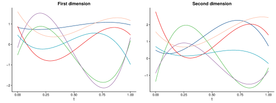
Figure 1: Six distinct two-dimensional curves simulated from Equation 16, each distinguished by a distinct color. The left side showcases dimension 1, while the right side displays dimension 2. The colors when functions arranged from bottom to top when $t=0$, are green, purple, cyan, red, blue and orange in the first dimension, and green, purple, blue, cyan, orange and red in the second dimension.

Table 1 provides a color assignment for curves based on various index values, ranging from bottom to top. Three different indexes, resulting in three separate columns, are considered. The first column represents the order given by MEI for each dimension individually. In this column, two values are presented: the first one corresponding to the curve achieving the given position in the first dimension, and the second one corresponding to the curve in the second dimension. This two-values representation arises because MEI is a one-dimensional index. Conversely, the remaining two columns refer to MEI and uMEI, both of which consider the multivariate nature of the curves and, therefore, yield a single value in each case.

Table 1: color assignment for index values (1-6) indicating the ranking from the lowest value (top row) to the highest value (bottom row). The first column displays the MEI values for each component (ME1 for the first dimension and MEI2 for the second dimension), while the last two columns represent the multivariate indexes MEI and uMEI.

Ordering	(MEI1, MEI2)	MEI	uMEI
1	(Green, Purple)	Cyan	Purple
2	(Red, Cyan)	Green	Cyan
3	(Cyan, Green)	Purple	Green
4	(Purple, Red)	Red	Red
5	(Orange, Blue)	Blue	Blue
6	(Blue, Orange)	Orange	Orange

First, it is of utmost importance to understand that the concepts of epigraph and hypograph indexes offer an ordering of the data from top to bottom or vice versa. Applying MEI to each data component gives a different order for each dimension, which overlooks the interrelations among them. In contrast, MEI gives a unified ordering for the entire dataset, taking into account these interrelations. In order to highlight the contrasting outcomes resulting from the inclusion or exclusion of these interrelations, we will undertake a comparative analysis of the ordering yielded by MEI, and the one assessed applying MEI dimension by dimension.

When each dimension is independently considered, the curves can be arranged based on their respective univariate indexes. Consequently, the application of the MEI in each dimension can lead to distinct orderings. This is evident in Table 1, where each row in the first column exhibits two colors, one for each dimension. In this example, no curves occupy the same position for both dimensions. This arises from the fact that any given row in the first column displays two identical colors, indicating that the order established when using the indexes dimension by dimension is entirely dissimilar in both dimensions.

In general, when calculating the indexes in a multivariate way, two things could happen:

• The position of a curve when ordering MEI is the one given by the univariate MEI for at least one dimension.

• The position of a curve when applying MEI does not coincide with the one given by MEI in any dimension.

Both scenarios are exemplified in the curves featured in Figure 1 and the corresponding results found in Table 1. The first scenario is evident in the last three curves, where the value of MEI coincides with the value obtained by MEI in the second dimension. In contrast, the second scenario occurs in the first three rows. In these instances, the two values generated by MEI differ from the value derived from MEI, resulting in distinct orderings. Hence, this implies that the extremeness of a curve is contingent upon whether the interdependencies between dimensions are considered. As a result, a curve may exhibit extremeness in a specific dimension but not as a multivariate curve.

Finally, we will examine the differences between uMEI given by Equation 3 with uniform weights, and MEI introduced in this paper and given by Equation 7. Both of them consider the multivariate nature of the curves. Their main difference lies in how they consider these curves. uMEI computes the average of MEI for all the dimensions, while MEI consider the multidimensional curves within the definition of the index. In this case, the ordering given by uMEI is the same as the one obtained by applying MEI to the second dimension. However, the ordering given by MEI does not exactly coincide with those achieved for any single dimension.

To summarize, in Figure 1, the curve achieving the minimum uMEI is the cyan one, and the curve achieving the minimum MEI is the purple one. If we consider these two curves as a whole, rather than as two independent curves, the cyan curve appears more extreme than the purple one. This underscores the importance of incorporating all dimensions of the curves within the index’s definition.

In conclusion, this example serves to highlight the significant influence of index definition on the resulting orderings.

2.4 Relation between indexes

This section aims to present the relationship between the definitions of the epigraph and hypograph indexes in the multivariate and the univariate cases. The multivariate definitions of the indexes, $\rho$MEI and $\rho$MHI, given by Ieva  Paganoni ¹⁸ (Equations 3 and 4) are obtained as a weighted average of the one-dimensional indexes, thereby establishing a direct connection between these multivariate definitions and their one-dimensional counterparts. However, the relationship between MEI and MHI (Equations 7 and 8) and MEI and MHI (Equations 12 and 13), and the relationship between MEI and MHI and $\rho$MEI and $\rho$MHI, warrant further examination.

A non-linear relationship can be established between MEI and MHI. Furthermore, this relationship depends on the one-dimensional counterparts, thus also establishing a connection with MEI and MHI. Given that $\rho$MEI and $\rho$MHI are defined as weighted averages of the one-dimensional counterparts, this leads to a relationship with $\rho$MEI and $\rho$MHI.

In the one-dimensional case, the aforementioned non-linear relationship is not achieved. Within functional datasets in one dimension, the relationship between MEI and MHI has been already established in Pulido . ³⁶, having that:

$$\text{MHI}_{n}(x)-\text{MEI}_{n}(x)=\frac{1}{n}.$$ (9)

However, for a multivariate functional dataset with $p>1$ dimensions, the relationship between these two indexes is shown to be dependent on the values of the indexes in previous dimensions. As a result, a non-constant relationship between the two indexes emerges. The following definitions and notation will be introduced to demonstrate this result:

$$A^{p}_{j_{1},\ldots,j_{r}}=\sum_{i=1}^{n}\frac{\lambda(\bigcap_{k=1}^{r}\{x_{ij_{k}}\geq x_{j_{k}}\})}{n\lambda(I)},$$ (10)

and

$$B^{p}_{j_{1},\ldots,j_{r}}=\sum_{i=1}^{n}\frac{\lambda(\bigcap_{k=1}^{r}\{x_{ij_{k}}\leq x_{j_{k}}\})}{n\lambda(I)},$$ (11)

where $p$ is the number of dimensions of the initial dataset, and $\{j_{1},\ldots,j_{r}\}\subseteq\{1,\ldots,p\}$ denote the $r$ dimensions to be considered to define the index with dimension $r$. These $r$ dimensions form a permutation of size $r$ from the $p$ dimensions of the original dataset. In light of the preceding notation, the indexes for a dataset consisting of $n$ functions in $p$ dimensions, are given as follows:

$$\mathbf{MEI}_{n}(\textbf{x})=1-A^{p}_{1,...,p},$$ (12)

and

$$\mathbf{MHI}_{n}(\textbf{x})=B^{p}_{1,...,p}.$$ (13)

Now, the notation $\mathbf{MEI}^{p}_{n,j_{1},...,j_{r}}$ and $\mathrm{MHI}^{p}_{n,j_{1},...,j_{r}}$ will be considered to denote the epigraph/hypograph indexes in dimension $r$ with $r\leq p$. The subset formed by $r$ of the $p$ dimensions conforming to the initial dataset, as mentioned before, will be denoted as $\{j_{1},\ldots,j_{r}\}$.

In that way,

$$\mathbf{MEI}^{p}_{n,j_{1},...,j_{r}}(\textbf{x})=1-A^{p}_{j_{1},...,j_{r}},$$ (14)

and

$$\mathbf{MHI}^{p}_{n,j_{1},...,j_{r}}(\textbf{x})=B^{p}_{j_{1},...,j_{r}},$$ (15)

If $r=p$, Equations 12 and 13 are particular cases of the Equations 14 and 15. Thus, in order to simplify the notation,

$$\mathbf{MEI}^{p}_{n,j_{1},...,j_{p}}(\textbf{x})=\mathbf{MEI}_{n}(\textbf{x}),$$

and

$$\mathbf{MHI}^{p}_{n,j_{1},...,j_{p}}(\textbf{x})=\mathbf{MHI}_{n}(\textbf{x}).$$

We are now poised to establish a relationship between the multivariate indexes, akin to the relationship observed in one dimension as defined by Equation 9.

Theorem 2.1.

The following relation between $\mathrm{MEI}_{n}$ and $\mathrm{MHI}_{n}$ holds for a dataset with $n$ curves in $p$ dimensions.

$$\mathbf{MHI}_{n}(\mathbf{x})+(-1)^{p+1}\mathbf{MEI}_{n}(\mathbf{x})=\sum_{r=1}^{p-1}\sum_{1\leq j_{1}<\ldots<j_{r}\leq p}^{p}(-1)^{r+p+1}\mathbf{MHI}^{p}_{n,j_{1},\ldots,j_{r}}(\mathbf{x})+(-1)^{p+1}\frac{1}{n}+(-1)^{p+1}R_{p},$$

where $R_{p}$ tends to 0 as $n$ tends to infinity.

Proof 2.2.

Applying the rules of probability and the definition of $B_{j_{1},\ldots,j_{r}}$ given by Equation 11:

$$\begin{split}B^{p}_{1,\ldots,p}&=(-1)^{p+1}\sum_{i=1}^{n}\frac{\lambda(\bigcup_{j=1}^{p}\{x_{ij}\leq x_{j}\})}{n\lambda(I)}+\sum_{r=1}^{p-1}\sum_{1\leq j_{1}<\ldots<j_{r}\leq p}^{p}(-1)^{r+p+1}B_{n,j_{1},\ldots,j_{r}}=\\ &(-1)^{p+1}\sum_{i=1}^{n}\frac{\lambda(\bigcup_{j=1}^{p}\{x_{ij}>x_{j}\}^{\mathsf{c}})}{n\lambda(I)}+\sum_{r=1}^{p-1}\sum_{1\leq j_{1}<\ldots<j_{r}\leq p}^{p}(-1)^{r+p+1}B_{n,j_{1},\ldots,j_{r}}=\\ &(-1)^{p+1}\sum_{i=1}^{n}\frac{\lambda(I)-\lambda(\bigcap_{j=1}^{p}\{x_{ij}>x_{j}\})}{n\lambda(I)}+\sum_{r=1}^{p-1}\sum_{1\leq j_{1}<\ldots<j_{r}\leq p}^{p}(-1)^{r+p+1}B_{n,j_{1},\ldots,j_{r}}=\\ &\sum_{r=1}^{p-1}\sum_{1\leq j_{1}<\ldots<j_{r}\leq p}^{p}(-1)^{r+p+1}B^{p}_{j_{1},\ldots,j_{r}}+(-1)^{p+1}+(-1)^{p}A^{p}_{1,\ldots p}+(-1)^{p+1}\frac{1}{n}+(-1)^{p+1}R_{p},\end{split}$$

where $R_{p}=\sum_{k=1}^{2^{p}-1}\sum_{\begin{subarray}{c}i=1\\ x_{i}\neq x\end{subarray}}^{n}\frac{C}{n\lambda(I)},$ with $C\in\mathcal{C}_{p}$, where $\mathcal{C}_{p}$ is the set of the Lebesgue measure of all the possible intersections of $p$ elements of the type $\{x_{ij}>x_{j}\}$ or $\{x_{ij}=x_{j}\}$, $j=1,\ldots,p$. It is important to note that the set $\mathcal{C}_{p}$ is composed by $2^{p}$ elements. Nevertheless, the above summation is taken up to $2^{p}-1$ since the intersection that contains all the elements of type $\{x_{ij}>x_{j}\}$ is included in the disaggregation of $B^{p}_{1,\ldots,p}$.

Finally, the following relation is obtained:

$$\mathbf{MHI}_{n}(\mathbf{x})+(-1)^{p+1}\mathbf{MEI}_{n}(\mathbf{x})=\sum_{r=1}^{p-1}\sum_{1\leq j_{1}<\ldots<j_{r}\leq p}^{p}(-1)^{r+p+1}\mathbf{MHI}^{p}_{n,j_{1},\ldots,j_{r}}(\mathbf{x})+(-1)^{p+1}\frac{1}{n}+(-1)^{p+1}R_{p},$$

where $R_{p}$ tends to 0 as $n$ tends to infinity.

Note that, when evaluating this expression for $p=1$, the corresponding equation for the one-dimensional case corresponds to Equation 9. With this general expression, the resulting equation is

$$\text{MHI}_{n}(x)-\text{MEI}_{n}(x)=\frac{1}{n}+R_{1}$$

. In this case, $R_{1}=\sum_{\begin{subarray}{c}i=1\\ x_{i}\neq x\end{subarray}}^{n}\frac{\lambda\{x_{i}=x\}}{n\lambda(I)}$, which tends to 0 when $n$ is big, obtaining the same result given in Pulido . ³⁶.

If the expression is now evaluated for $p=2$, then:

$$\mathbf{MHI}_{n}(\mathbf{x})+\mathbf{MEI}_{n}(\mathbf{x})=\mathbf{MHI}^{2}_{1}(\mathbf{x})+\mathbf{MHI}^{2}_{2}(\mathbf{x})-\frac{1}{n}-R_{2}.$$

For $p=3$, the relationship will be given by:

$$\mathbf{MHI}_{n}(\mathbf{x})-\mathbf{MEI}_{n}(\mathbf{x})=\mathbf{MHI}^{3}_{n,1,2}(\mathbf{x})+\mathbf{MHI}^{3}_{n,1,3}(\mathbf{x})+\mathbf{MHI}^{3}_{n,2,3}(\mathbf{x})-\mathbf{MHI}^{3}_{n,1}(\mathbf{x})-\mathbf{MHI}^{3}_{n,2}(\mathbf{x})-\mathbf{MHI}^{3}_{n,3}(\mathbf{x})+\frac{1}{n}+R_{3}.$$

In order to facilitate comprehension of the general case, the proof when $p=3$ is deferred to the Appendix.

In summary, Theorem 2.1 establishes the relationship between MEI and MHI for multivariate functional data. It demonstrates that this relationship remains constant for the one-dimensional case (Equation 9). However, for any value of $p>1$, the relationship depends on the indexes of previous dimensions. Note that one of the terms is $\sum_{i=1}^{p}\mathbf{MHI}_{n,i}^{p}$, which represents the sum of the generalized epigraph indexes in one dimension. It is this term the one that makes it possible the establishment of a connection not only with the one dimensional indexes (MEI and MHI) but also with the multivariate definitions introduced by Ieva  Paganoni ¹⁸ ($\rho$MEI and $\rho$MHI).

The primary contributions of this work encompass the introduction of novel multivariate indexes definitions and their subsequent utilization in clustering multivariate functional data. The exploration of the second contribution will be delved into further detail in Section 3. It is noteworthy at this point that the one-dimensional indexes were applied in Pulido . ³⁶ to transform a functional database into a multivariate one. In that context, the use of MHI was omitted due to the linear dependence between MEI and MHI. However, when considering MEI and MHI for transforming a multivariate functional database into a multivariate one, it is important that the difference between MEI and MHI is not a constant value, as was the case in the one-dimensional scenario. Consequently, both indexes can be concurrently employed.

2.5 Properties of the multivariate epigraph and hypograph indexes

This section outlines several properties satisfied by EI, HI, MEI and MHI as given by Equations 5, 6, 7 and 8 respectively. They follow the line of López-Pintado  Romo ²⁸, Ieva  Paganoni ¹⁷, López-Pintado . ²⁷, and Franco-Pereira  Lillo ¹². The proofs of these results are deferred to the Appendix.

Proposition 2.3.

The EI and HI with respect to a set of functions $\mathbf{x_{1}}(t),$ … $\mathbf{x_{n}}(t)$ are invariant under the following transformations:

• Let $\mathbf{T}(\mathbf{x})$ be the transformation function defined as $\mathbf{T}(\mathbf{x}(t))=\mathbf{A}(t)\mathbf{x}(t)+\mathbf{b}(t),$ where $t\in\mathcal{I}$ and $\mathbf{A}(t)$ is a $p\times p$ invertible matrix with $A_{ij}(t)$ a continuous function in $t$ with $t\in\mathcal{I}$ and $\mathbf{b}(t)\in C(\mathcal{I},\mathbb{R}^{p})$. Then,

  $$\mathbf{EI}(\mathbf{T}(\mathbf{x}))=\mathbf{EI}(\mathbf{x}),\ \mathrm{and,}$$

  $$\mathbf{HI}(\mathbf{T}(\mathbf{x}))=\mathbf{HI}(\mathbf{x}).$$

• Let $g$ be a one-to-one transformation of the interval $\mathcal{I}$. Then,

  $$\mathbf{EI}(\mathbf{x}(g))=\mathbf{EI}(\mathbf{x}),\ \mathrm{and,}$$

  $$\mathbf{HI}(\mathbf{x}(g))=\mathbf{HI}(\mathbf{x}).$$

The following proposition establishes similar properties as those mentioned in Proposition 2.3, but now for the generalized indexes.

Proposition 2.4.

The MEI and MHI with respect to a set of functions $\mathbf{x_{1}}(t),$ … $\mathbf{x_{n}}(t)$ are invariant under the following transformations:

• Let $\mathbf{T}(\mathbf{x})$ be the transformation function defined as $\mathbf{T}(\mathbf{x}(t))=\mathbf{A}(t)\mathbf{x}(t)+\mathbf{b}(t),$ where $t\in\mathcal{I}$ and $\mathbf{A}(t)$ is a $p\times p$ invertible matrix with $A_{ij}(t)$ a continuous function in $t$ with $t\in\mathcal{I}$ and $\mathbf{b}(t)\in C(\mathcal{I},\mathbb{R}^{p})$. Then,

  $$\mathbf{MEI}(\mathbf{T}(\mathbf{x}))=\mathbf{MEI}(\mathbf{x}),\ \mathrm{and,}$$

  $$\mathbf{MHI}(\mathbf{T}(\mathbf{x}))=\mathbf{MHI}(\mathbf{x}).$$

• Let $g$ be a one-to-one transformation of the interval $\mathcal{I}$. Then,

  $$\mathbf{MEI}(\mathbf{x}(g))=\mathbf{MEI}(\mathbf{x}),\ \mathrm{and,}$$

  $$\mathbf{MHI}(\mathbf{x}(g))=\mathbf{MHI}(\mathbf{x}).$$

The proposition below considers these indexes as a measure of extremity. The objective is to demonstrate that these indexes are suitable for ordering functions, as discussed in Section 1. Specifically, EI arranges the sample of functions from bottom (EI equal to 0) to top (EI equal to 1). On the other hand, for HI, 1-HI is considered, where a value of 1 implies that there are no curves below it. Consequently, this index orders functions from top (1-HI equal to 0) to bottom (1-HI equal to 1).

Proposition 2.5.

The maximum between $\mathbf{EI}_{n}(\mathbf{x})$ and $1-\mathbf{HI}_{n}(\mathbf{x})$ converges almost surely to one as the supreme norm of one of the components of the multivariate process $\mathbf{x}$ tend to infinity:

$$\underset{\min_{k=1,...,p}\lVert x_{k}\rVert_{\infty}\geq M}{sup}\max\{\mathbf{EI}_{n}(\mathbf{x},P_{\mathbf{X}}),1-\mathbf{HI}_{n}(\mathbf{x},P_{\mathbf{X}})\}\overset{a.s}{\to}1,$$

when $\ M\to\infty,$ where $\lVert x_{k}\rVert_{\infty}$ is the supreme norm of the $kth$ component of $\mathbf{x}$.

The following proposition provides the strong consistency for EI and HI.

Proposition 2.6.

$\mathbf{EI}_{n}$ and $\mathbf{HI}_{n}$ are strongly consistent.

• $\mathbf{EI}_{n}$ is strongly consistent.

  $$\mathbf{EI}_{n}(\mathbf{x})\overset{a.s}{\to}\mathbf{EI}(\mathbf{x},P_{\mathbf{X}}),\ as\ n\to\infty.$$

• $\mathbf{HI}_{n}$ is strongly consistent.

  $$\mathbf{HI}_{n}(\mathbf{x})\overset{a.s}{\to}\mathbf{HI}(\mathbf{x},P_{\mathbf{X}}),\ as\ n\to\infty.$$

Proof 2.7.

The proof is a consequence of the law of large numbers.

Finally, from Propositions 2.5 and 2.6, the following result holds:

Proposition 2.8.

The maximum between $\mathbf{EI}(\mathbf{x},P_{\mathbf{X}})$ and $1-\mathbf{HI}(\mathbf{x},P_{\mathbf{X}})$ converges to one as the supreme norm of one of the components of the multivariate process $\mathbf{x}$ tend to infinity:

$$\underset{\min_{k=1,...,p}\lVert x_{k}\rVert_{\infty}\geq M}{sup}\max\{\mathbf{EI}(\mathbf{x},P_{\mathbf{X}}),1-\mathbf{HI}(\mathbf{x},P_{\mathbf{X}})\}\to 1,$$

when $\ M\to\infty,$ where $\lVert x_{k}\rVert_{\infty}$ is the supreme norm of the $kth$ component of $\mathbf{x}$.

3 Clustering multivariate functional data

The indexes MEI and MHI naturally enable the adaptation of the methodology proposed in Pulido . ³⁶ for clustering one-dimensional functional data to the multivariate context. In this section, we will provide an outline of this expansion, as well as an overview of various existing methods in the literature designed for clustering multivariate functional data. Subsequently, in the following sections, we will apply the proposed approach to various simulated and real datasets. Moreover, we will conduct a comparative analysis of the obtained results against those achieved by other established methodologies in the literature.

3.1 EHyClus for multivariate functional data

The methodology proposed in Pulido . ³⁶, known as EHyClus, consists of four main steps, illustrated by Figure 2. This approach transforms the original functional dataset into a multivariate one by applying the epigraph and hypograph indexes in one dimension to the original curves, along with their first and second derivatives. Then, different multivariate clustering approaches are fitted to that dataset. Finally, a clustering partition is obtained as the combination of different indexes and one clustering methodology. See Pulido . ³⁶ for more details.

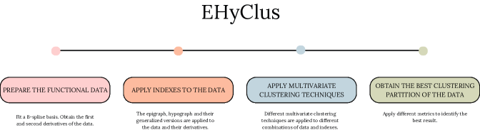
Figure 2: Strategy followed by EHyClus methodology

In order to adapt EHyClus for the context of multivariate functional data, a modification is necessary in the second step illustrated in Figure 2, which involves applying indexes to the data. This adjustment is needed to accommodate the multivariate dataset. There are several options for defining multivariate indexes, including those introduced in this study (MEI and MHI), but also those proposed by Ieva  Paganoni ¹⁸ ($\rho$MEI and $\rho$MHI, with customizable weights, or any other option.

In the one-dimensional case, the multivariate clustering techniques are applied to different combinations of the EI, HI and MEI of the curves and their first and second derivatives. Note that, MHI was discarded because of the linear relation existing between MEI and MHI. In the multivariate context, EI and HI are really restrictive and result, in almost all cases, in values so close to 1 and 0 respectively. This, added to the absence of a linear relation between MEI and MHI (see Section 2.4), leads to only consider MEI and MHI. A total of 15 different combinations of data, first and second derivatives with indexes (Table 2) have been considered. In this table, the notation used can be expressed as (b).(c) where (b) represent the data combinations, being ‘_’ the curves, ‘d’ first derivatives and ‘d2’ second derivatives, and (c) represents the indexes that have been used. Once these 15 datasets are created, 12 different multivariate clustering techniques have been applied to each of them. These methods include different hierarchical clustering approaches with Euclidean distance, such as single linkage, complete linkage, average linkage and centroid linkage for calculating similarities between clusters, and Ward method (Murtagh  Contreras ³²); k-means with Euclidean and Mahalanobis distances (Jain ²⁴); kernel k-means (kkmeans) with Gaussian and polynomial kernels (Dhillon . ¹⁰); spectral clustering (spc) (Von Luxburg ⁴⁴) and support vector clustering (svc) with k-means and kernel k-means (Ben-Hur . ³). All these combinations result in 180 different cluster results denoted as (a).(b).(c) where (a) stands for the clustering method as represented in Table 3. Finally, to assess the classification performance, three different external validation strategies will be employed: Purity, F-measure and Rand Index (RI). These validation metrics are comprehensively explained in Manning . ²⁹, and Rendón . ³⁸.

Table 2: Notation and description of the combinations of data and indexes.

Notation	Description
_.MEIMHI = (MEI, MHI)	The modified epigraph and the hypograph index on the original curves.
d.MEIMHI = (dMEI, dMHI)	The modified epigraph and the hypograph index on the first derivatives.
d2.MEIMHI = (d2MEI, d2MHI)	The modified epigraph and the hypograph index on the second derivatives.
_d.MEIMHI = (MEI, MHI, dMEI, dMHI)	The modified epigraph and the hypograph index on the original curves and on the first derivatives.
_d2.MEIMHI = (MEI, MHI, d2MEI, d2MHI)	The modified epigraph and the hypograph index on the original curves and on the second derivatives.
dd2.MEIMHI = (dMEI, dMHI, d2MEI, d2MHI)	The modified epigraph and the hypograph index on the first and on the second derivatives.
_dd2.MEIMHI = (MEI, MHI, dMEI, dMHI, d2MEI, d2MHI)	The modified epigraph and the hypograph index on the original curves, first and second derivatives.
_d.MEI = (MEI, dMEI)	The modified epigraph index on the original curves and first derivatives.
_d2.MEI = (MEI,d2MEI)	The modified epigraph index on the original curves and on the second derivatives.
dd2.MEI = (dMEI, d2MEI)	The modified epigraph index on the first and on the second derivatives.
_dd2.MEI = (MEI, dMEI, d2MEI)	The modified epigraph index on the original curves, first and second derivatives.
_d.MHI = (MHI, dMHI)	The modified hypograph index on the original curves and on the first derivatives.
_d2.MHI = (MHI, d2MHI)	The modified hypograph index on the original curves and on the second derivatives.
dd2.MHI = (dMHI, d2MHI)	The modified hypograph index on the first and son the econd derivatives.
_dd2.MHI = (MHI, dMHI, d2MHI)	The modified hypograph index on the original curves, first and second derivatives.

Table 3: Notation and description of the clustering method applied to the dataset obtained from the combination of data and indexes given by (b).(c).

Notation	Description
single.(b).(c)	Hierarchical clustering with single linkage and Euclidean distance.
complete.(b).(c)	Hierarchical clustering with complete linkage and Euclidean distance.
average.(b).(c)	Hierarchical clustering with average linkage and Euclidean distance.
centroid.(b).(c)	Hierarchical clustering with centroid linkage and Euclidean distance.
ward.D2.(b).(c)	Hierarchical clustering with Ward method and Euclidean distance.
kmeans.(b).(c)-euclidean	k-means clustering with Euclidean distance.
kmeans.(b).(c)-mahalanobis	k-means clustering with Mahalanobis distance.
kkmeans.(b).(c)-gaussian	kernel k-means clustering with a Gaussian kernel.
kkmeans.(b).(c)-polynomial	kernel k-means clustering with a polynomial kernel.
spc.(b).(c)	spectral clustering.
svc.(b).(c)-kmeans	support vector clustering with k-means initialization.
svc.(b).(c)-kkmeans	support vector clustering with kernel k-means initialization.

3.2 Clustering methods for multivariate functional data in the literature

In this section, we present several existing approaches from the literature for clustering multivariate functional data. The outcomes of these approaches will be compared to the results of EHyClus. For benchmarking purposes, six distinct methods from the literature have been selected. Furthermore, to ascertain whether MEI and MHI offer more insights about the data compared to $\rho$MEI and $\rho$MHI, EHyClus as explained in Section 3.1, has also been tested applying uMEI and uMHI (uniform weights) and cMEI and cMHI (weights based on the covariance matrices).

The first method for benchmarking is funclust algorithm, from Funclustering R package, fully explained in Jacques  Preda ²³. It is the first model-based approach for clustering multivariate functional data in the literature. This approach apply multivariate functional principal component analysis to the data, to posteriorly fit a parametric mixture model based on the assumption of normality of the principal component scores. One of the weaknesses of this strategy is that only a given proportion of principal components is modelled, leading to ignore some available information. This limitation is overcome by funHDDC algorithm, fully explained in Schmutz . ⁴⁰, and available in the funHDDC R package. This methodology extends the latter by modelling all principal components with estimated variance different from zero. The next methodology is the FGRC method, described in Yamamoto  Hwang ⁴⁶. This strategy proposes a clustering method for multivariate functional data which combines a subspace separation technique with functional subspace clustering. It tries to avoid the clustering process to be affected by the variances among functions restricted to regions that are not related to true cluster structure. Then, kmeans-d1 and kmeans-d2 are two approaches described in Ieva  Paganoni ¹⁷. They are two different implementations of k-means, which basically differ in the distance considered between the multivariate curves. kmeans-d1 uses the norm in the Hilbert space $L^{2}(\mathcal{I},\mathbb{R}^{p})$, while kmeans-d2 considers the norm in the Hilbert space $H^{1}(\mathcal{I},\mathbb{R}^{p})$. Finally, the methodology proposed in Martino . ³¹ and available in the R package gmfd, is also tested. This one is also based on k-means clustering, but in this case, a generalized Mahalanobis distance for functional data, $d_{\rho}$ where the value of $\rho$ has to be set in advance is employed.

In this paper, we will refer to these six techniques respectively as: Funclust, funHDDC, FGRC, kmeans-d1, kmeans-d2 and gmfd-kmeans. Finally, EHyClus will refer to the methodology proposed in this work using MEI and MHI. EHyClus-mean will denote EHyClus with uMEI and uMHI, and EHyClus-cov will consider the use of $\rho$MEI and $\rho$MHI.

4 Simulation study

This section encompasses numerical experiments aimed at illustrating the performance of the proposed methodology and comparing it with the existing approaches in the literature, explained in Section 3.2. These experiments serve to demonstrate the behavior and effectiveness of the proposed methodology in contrast to some other approaches available for clustering multivariate functional data. Four different datasets are simulated for this purpose, two, (DS1 and DS2) with two groups and another two (DS3 and DS4) with four groups.

DS1 first appears in Martino . ³¹, and it is the extension of a one-dimensional example considered in the same work, which have been also employed in Pulido . ³⁶ for clustering functional data in one dimension. It consists of two functional samples of size 50 defined in $[0,1]$, with continuous trajectories generated by independent stochastic processes in $L^{2}(\mathcal{I}^{2})$. Each component of the curve is evaluated in 150 equidistant observations in the interval $[0,1]$.

The 50 functions of the first sample are generated as follows:

$$\mathbf{X}_{1}(t)=\mathbf{E}_{1}(t)+\sum_{k=1}^{100}\mathbf{Z}_{k}\sqrt{\rho_{k}}\theta_{k}(t),$$ (16)

where $\mathbf{E}_{1}(t)=\begin{pmatrix}t(1-t)\\ 4t^{2}(1-t)\end{pmatrix}$ is the mean function of this process, $\{\mathbf{Z}_{k},k=1,...,100\}$ are independent bivariate normal random variables, with mean $\mathbf{\mu=0}$ and covariance matrix $\Sigma=\begin{pmatrix}1&0.5\\ 0.5&1\end{pmatrix},$ and $\{\rho_{k},k\geq 1\}$ is a positive real numbers sequence defined as

$$\rho_{k}=\left\{\begin{array}[]{lll}\frac{1}{k+1}&if&k\in\{1,2,3\},\\ \frac{1}{{(k+1)}^{2}}&if&k\geq 4,\end{array}\right.$$

in such a way that the values of $\rho_{k}$ are chosen to decrease faster when $k\geq 4$ in order to have most of the variance explained by the first three principal components. Finally, the sequence $\{\theta_{k},k\geq 1\}$ is an orthonormal basis of $L^{2}(I)$ defined as

$$\theta_{k}(t)=\left\{\begin{array}[]{lllll}I_{[0,1]}(t)&if&k=1,&\\ \sqrt{2}\sin{(k\pi t)}I_{[0,1]}(t)&if&k\geq 2,\\ &&k\ even,\\ \sqrt{2}\cos{((k-1)\pi t)}I_{[0,1]}(t)&if&k\geq 3,\\ &&k\ odd,\end{array}\right.$$

where $I_{A}(t)$ stands for the indicator function of set $A$.

The 50 functions of the second sample are generated by $\mathbf{X}_{2}(t)=\mathbf{E}_{2}(t)+\displaystyle\sum_{k=1}^{100}\mathbf{Z}_{k}\sqrt{\rho_{k}}\theta_{k}(t),$ where $\mathbf{E}_{2}(t)=\mathbf{E}_{1}(t)+\mathbf{1}\displaystyle\sum_{k=4}^{100}\sqrt{\rho_{k}}\theta_{k}(t),$ is the mean function of this process, where $\mathbf{1}$ represents a vector of 1s.

The first step of EHyClus consists of smoothing the data (see Figure 2) with a cubic B-spline basis in order to remove noise and to be able to use its first and second derivatives. A sensitivity analysis regarding the best number of basis was already performed in Pulido . ³⁶, leading to the conclusion that a number of basis between 30 and 40 should be considered. In this work, we will use 35 basis.

As shown in Figure 3, there is a significant overlap between the two groups in both dimensions. Therefore, it is difficult to distinguish the two groups visually. Figures 4 and 5 represent the mean curves of each of the two groups for the original curves and the first derivatives for each dimension to distinguish the behavior of the two groups. However, upon examining the indices representation depicted in Figure 6, it becomes evident that the two groups can be readily discerned. The figure illustrates the utilization of MEI and MHI over the first derivatives. This representation has been executed in a two-dimensional format to enhance clarity of visualization. While it is conceivable to present a scatter plot in dimension four, corresponding to the most effective approach in Table 4 and including MEI and MHI for both first and second derivatives, comprehension may prove challenging.

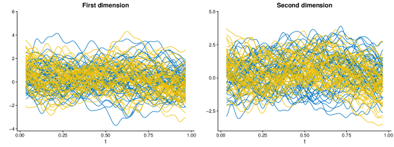
Figure 3: DS1 data. Dimension 1 (left panel) and 2 (right panel).

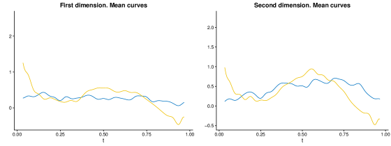
Figure 4: Mean curves of the two groups of DS1. Dimension 1 (left panel) and 2 (right panel).

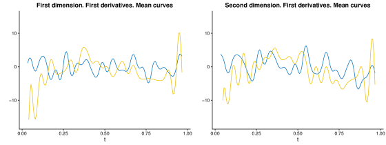
Figure 5: Mean curves of the two groups of DS1 derivatives. Dimension 1 (left panel) and 2 (right panel).

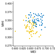
Figure 6: Scatter plot of the modified epigraph index (MEI) and the modified hypograph index (MHI) of the first derivatives of DS1.

When applying EHyClus with MEI and MHI as explained in Section 3.1, 180 different combinations of models and indexes are considered. Here, DS1 data have been simulated 100 times, and the better 5 combinations, based on the mean RI, are shown in Table 4. These five combinations are achieved when considering only the derivatives of the data applied to both MEI and MHI, without taking the original curves into consideration. Thus, the differences in these results only depend on the multivariate clustering method to be considered. In the case of the best methodology, the clustering method is k-means with Euclidean distance, but it obtains almost the same results as considering Mahalanobis distance, both with a mean RI equal to 0.9698.

Table 4: Top 5 mean results for DS1 with EHyClus on 100 simulations.

	Purity	Fmeasure	RI	Time
kmeans.dd2.MEIMHI-euclidean	0.9846	0.9695	0.9698	0.00262
kmeans.dd2.MEIMHI-mahalanobis	0.9846	0.9695	0.9698	0.00281
svc.dd2.MEIMHI-mlKmeans	0.9725	0.9559	0.9559	0.00395
svc.dd2.MEIMHI-kmeans	0.97250	0.9557	0.9556	0.00369
ward.D2.dd2.MEIMHI-euclidean	0.9724	0.9474	0.9475	0.00038

Afterwards, all the existing procedures that were reviewed in Section 3.2 are applied to DS1. Following the same structure as before, the mean results of 100 simulations are reflected in Table 5. Note that these table represents the best approach of each methodology. Between these methods, kmeans-d2 is the one obtaining the best value equal to 0.9009, near to 0.07 units below the best approach offered by EHyClus (Table 4). Furthermore, the next approach would be Funclust with 0.8198, close to 0.15 units below the proposed approach in this paper. The other approaches do not obtain competitive results in terms of RI. In terms of execution time, EHyClus is the fastest between those competing in RI values.

Table 5: Mean values for DS1 of Purity, F-measure, Rand Index (RI) and execution time for all the competitors models on 100 simulations.

	Purity	Fmeasure	RI	Time
EHyClus-mean	0.7243	0.5986	0.6005	0.0106
EHyClus-cov	0.7237	0.5977	0.5997	0.0104
Funclust	0.8563	0.8197	0.8198	1.3277
funHDDC	0.5810	0.5217	0.5157	3.6154
FGCR	0.5749	0.5070	0.5063	0.2275
kmeans-d1	0.5635	0.4021	0.5034	0.1244
kmeans-d2	0.9964	0.8878	0.9009	0.1211
gmfd-kmeans	0.7400	0.6949	0.6678	3.3498

Figure 7 summarizes all the applied methodologies in terms of RI. This figure shows the distribution of RI for each methodology. Funclust and gmfd-kmeans are two approaches that, even in some cases they achieve almost perfect results, they have huge dispersion. An additional noteworthy observation is that when comparing EHyClus-cov and EHyClus-mean in relation to their mean RI, they yield nearly identical values. However, upon comparing their distributions, it becomes evident that EHyClus-cov exhibits greater symmetry and less dispersion, albeit resulting in a slightly lower mean value. Overall, EHyClus is the methodology with higher mean and median values, as well as the less disperse, leading to consider this methodology as the more accurate in terms of RI.

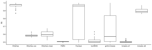
Figure 7: Boxplot of the RI for DS1 over 100 simulation runs of EHyClus and its competitors.

The second dataset (DS2) is based on a bivariate dataset with two groups appearing in Jacques  Preda ²³. In this case, 100 curves in $[1,21]$ are considered, 50 from each of the two groups, as follows:

1. $X_{1}(t)=-5+t/2+U_{2}h_{3}(t)+U_{3}h_{2}(t)+\sqrt{0.1}\epsilon(t),$
   $X_{2}(t)=-5+t/2+U_{1}h_{1}(t)+U_{2}h_{2}(t)+U_{3}h_{3}(t)+\sqrt{0.5}\epsilon(t),$

2. $X_{1}(t)=U_{3}h_{2}(t)+\sqrt{10}\epsilon(t),$
   $X_{2}(t)=U_{1}h_{1}(t)+U_{3}h_{3}(t)+\sqrt{0.5}\epsilon(t),$

where $U_{1}\sim\mathcal{U}(0.5,1/12)$, $U_{2}\sim\mathcal{U}(0,1/12)$ and $U_{3}\sim\mathcal{U}(0,2/3)$ are independent Gaussian variables and $\epsilon(t)$ represents a white noise independent of $U_{i},$ $i=1,2,3,$ with unit variance. The functions$h_{1}$, $h_{2}$ and $h_{3}$ are defined as $h_{1}(t)=(6-|t-11|)_{+}$, $h_{2}(t)=(6-|t-7|)_{+}$ and $h_{3}(t)=(6-|t-15|)_{+}$, being $(\centerdot)_{+}$ the positive part. The curves are observed in 1001 equidistant points of the interval $[1,21]$. The functions have been fitted with 35 cubic B-splines basis.

The curves and its first derivatives for the two dimensions of the data are presented in Figures 8 and 9. The curves are highly mixed, but most pronounce overlap occurs in the derivatives. Figure 10 represents the mean curves of the first derivatives over the two groups, showing the differences between them. This figure shows that the two groups present different behaviors, leading to be really well distinguishable when considering the indexes, as represented in Figure 11.

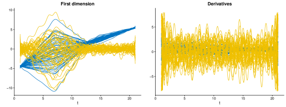
Figure 8: Dimension 1 of DS2 data. Original curves (left) and first derivatives (right).

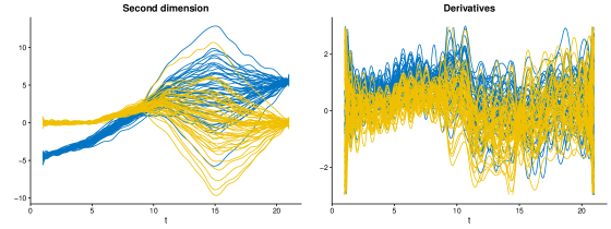
Figure 9: Dimension 2 of DS2 data. Original curves (left) and first derivatives (right).

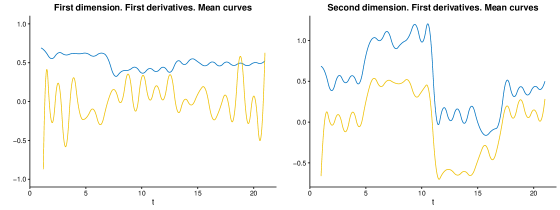
Figure 10: Mean curves of the four groups of DS2 derivatives. Dimension 1 (left) and 2 (right).

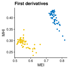
Figure 11: Scatter plot of the modified epigraph index (MEI) and the modified hypograph index (MHI) of the first derivatives of DS2.

When applying EHyClus to DS2, the results in Table 6 show that there are more than 15 different combination of data, indexes and cluster methodology obtaining perfect results for all the three metrics considered: Purity, F-measure and RI. All the combinations leading to these perfect results include the indexes applied to the first derivatives. Figure 11 represents the two groups when applying MEI and MHI to the first derivatives of the data. The two groups in this figure are really well separated, and they are easily distinguishable by any cluster method. Moreover, these top combinations sometimes include the indexes over the first and the second derivatives. This means that a four variables dataset is taken to apply the clustering techniques instead of a two variables one. The four indexes dataset is not illustrated here because it would be a four dimensional plot, really difficult to represent and understand.

Table 6: Top 15 mean results for DS2 with EHyClus on 100 simulations, obtaining perfect metrics values.

	Purity	Fmeasure	RI	Time
average.d.MEIMHI-euclidean	1	1	1	0.00100
average.dd2.MEIMHI-euclidean	1	1	1	0.00111
centroid.d.MEIMHI-euclidean	1	1	1	0.00241
centroid.dd2.MEIMHI-euclidean	1	1	1	0.00120
kkmeans.d.MEIMHI-polydot	1	1	1	0.02850
kkmeans.dd2.MEIMHI-polydot	1	1	1	0.03012
kmeans.d.MEIMHI-euclidean	1	1	1	0.00823
kmeans.d.MEIMHI-mahalanobis	1	1	1	0.00764
kmeans.dd2.MEIMHI-euclidean	1	1	1	0.00739
kmeans.dd2.MEIMHI-mahalanobis	1	1	1	0.00841
single.d.MEIMHI-euclidean	1	1	1	0.00109
single.dd2.MEIMHI-euclidean	1	1	1	0.00130
spc.d.MEIMHI	1	1	1	0.20115
spc.dd2.MEIMHI	1	1	1	0.19836
svc.d.MEIMHI-kmeans	1	1	1	0.01042

On the other hand, when applying the seven methodologies considered for comparisons, only two of them are able to compete with the results obtained by EHyClus. These results are presented in Table 7 and confirm that only EHyClus-mean, EHyClus-cov and funHDDC are able to compete with the results achieved by EHyClus (Table 6). Nevertheless, in the case of funHDDC, the execution time is high in comparison to those achieved by EHyClus with any index definition. When applying EHyClus with the alternative definitions of the indexes, again more than 15 combinations achieve perfect results concerning Purity, F-measure and RI. This fact out stand again that EHyClus is able to outperform other methodologies for clustering multivariate functional data.

Table 7: Mean values for DS2 of Purity, F-measure, Rand Index (RI) and execution time for all the competitors models on 100 simulations.

	Purity	Fmeasure	RI	Time
EHyClus-mean	1.0000	1.0000	1.0000	0.0003
EHyClus-cov	1.0000	1.0000	1.0000	0.0003
Funclust	0.8386	0.8254	0.8062	4.8313
funHDDC	0.9897	0.9808	0.9808	5.8811
FGRC	0.8228	0.7839	0.7836	8.8738
kmeans-d1	0.7775	0.7153	0.7165	0.0578
kmeans-d2	0.7618	0.6662	0.6671	0.0606
gmfd-kmeans	0.7211	0.6872	0.6649	53.7121

Finally, Figure 12 represents the RI distribution of each of the best approaches for each of the eight considered methodologies. EHyClus always obtains a RI equal to 1 for the three definitions of indexes available in Section 2.2. funHDDC also obtains almost all values equal to 1 in the 100 simulations. Nevertheless, it presents some outliers with a slower RI. This implies that this approach does not obtain a mean RI equal to 1 in Table 7. The remaining five methodologies obtain much more disperse results, with means much smaller than the other three approaches. Overall, EHyClus seems to be the best approach in this case.

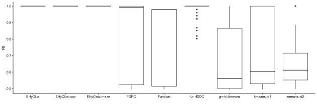
Figure 12: Boxplot of the RI for DS2 over 100 simulation runs of EHyClus and its competitors.

The third dataset (DS3) has been previously considered by Schmutz . ⁴⁰ to test their clustering algorithm. It is based on the data described in Bouveyron . ⁶, but changing the number of functions, the variance and adding a new dimension to the data. It consists of 1000 bivariate curves equally distributed in four different groups defined in $[1,21]$, generated as follows:

1. $X_{1}(t)=U+(1-U)h_{1}(t)+\epsilon(t),$
   $X_{2}(t)=U+(0.5-U)h_{1}(t)+\epsilon(t),$

2. $X_{1}(t)=U+(1-U)h_{2}(t)+\epsilon(t),$
   $X_{2}(t)=U+(0.5-U)h_{2}(t)+\epsilon(t),$

3. $X_{1}(t)=U+(0.5-U)h_{1}(t)+\epsilon(t),$
   $X_{2}(t)=U+(1-U)h_{1}(t)+\epsilon(t),$

4. $X_{1}(t)=U+(0.5-U)h_{2}(t)+\epsilon(t),$
   $X_{2}(t)=U+(1-U)h_{2}(t)+\epsilon(t),$

where $U\sim\mathcal{U}(0,0.1)$, $\epsilon(t)$ represents a white noise independent of $U$ with variance equal to $0.25$, and the functions $h_{1}$ and $h_{2}$ are defined as

$$h_{1}(t)=(6-|t-7|)_{+}\quad\mathrm{and}\quad h_{2}(t)=(6-|t-15|)_{+}.$$ (17)

The curves are observed in 101 equidistant points of the interval $[1,21]$. The functions have been fitted with 35 cubic B-splines basis. Then, the derivatives have been calculated, obtaining the curves represented in Figures 13 and 14, where original curves and first derivatives are represented for the two dimensions of the data.

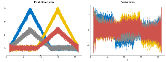
Figure 13: Dimension 1 of DS3 data. Original curves (left) and first derivatives (right).

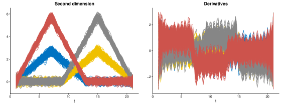
Figure 14: Dimension 2 of DS3 data. Original curves (left) and first derivatives (right).

The outcomes derived from the application of EHyClus and eight alternative methodologies to this dataset are presented in Table 8. Surprisingly, EHyClus produces the most favorable result when operating on the derivatives, and not on the original curves, obtaining the optimal combination employing k-means clustering on MEI and MHI derived from the first derivatives of the data. This finding is unexpected, as an examination of the curves displayed in Figures 13 and 14 reveals that the groups are more distinguishable in the original curves compared to the derivatives. Nevertheless, upon evaluating the indices depicted in Figure 15, it becomes apparent that the indexes associated with the original curves only manage to discriminate between two groups, whereas the indexes based on the derivatives successfully differentiate all four groups. This phenomenon may be attributed to the fact that, owing to the shape of the derivatives, the disparity in the number of curves situated below and above a particular one provides a more effective discriminative capacity than in the case of the original curves. It is noteworthy that the methodology introduced by Schmutz . ⁴⁰, referred to as funHDDC, achieves exceptionally high results, far from those obtained by all the other approaches. When comparing all the alternatives to funHDDC (0.99844 mean RI), EHyClus is the next best approach (0.88277 mean RI), far from Funclust (0.83591 mean RI), which is the following best value. Note that the execution time of funHDDC is really high compared to all the other approaches, being more than one thousand times slower than EHyClus and almost 5 times slower than Funclust.

Table 8: Mean values for DS3 of Purity, F-measure, Rand Index (RI) and execution time for EHyClus and all the competitors models on 100 simulations.

	Purity	Fmeasure	RI	Time
EHyClus	0.81308	0.76515	0.88277	0.01423
RHyClus-cov	0.40440	0.29890	0.64860	0.00970
EHyClus-mean	0.39877	0.31863	0.65815	0.05580
Funclust	0.70936	0.7674	0.83591	3.42640
funHDDC	0.99750	0.99737	0.99844	15.9790
FGRC	0.65151	0.63691	0.81316	6.38450
kmeans-d1	0.49026	0.46950	0.73467	0.48181
kmeans-d2	0.35296	0.32660	0.66260	0.44237
gmfd-kmeans	0.48420	0.59104	0.66568	0.46780

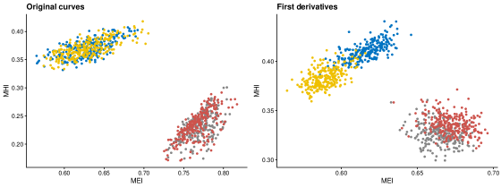
Figure 15: Scatter plots of the modified epigraph index (MEI) and the modified hypograph index (MHI) of DS3. Original data (left panel) and first derivatives (right panel).

The preceding analysis conducted on DS3 was carried out using the dataset selected in Schmutz . ⁴⁰. The funHDDC methodology proposed in that research yielded remarkably high outcomes. To gain further understanding of how EHyClus operates with four groups, and to elucidate how funHDDC works in different scenarios, we believe it would be interesting to modify certain parameters in the formulation of DS3 and observe the resulting effects. Consequently, a new dataset, referred to as DS4, has been generated. DS4 comprises 100 bivariate curves equally distributed in four different groups defined in $[1,21]$, generated as follows:

1. $X_{1}(t)=U+(1.5-U)h_{1}(t)+\epsilon(t),$
   $X_{2}(t)=U+(1-U)h_{1}(t)+\epsilon(t),$

2. $X_{1}(t)=U+(1-U)h_{2}(t)+\epsilon(t),$
   $X_{2}(t)=U+(0.5-U)h_{2}(t)+\epsilon(t),$

3. $X_{1}(t)=U+(1-U)h_{1}(t)+\epsilon(t),$
   $X_{2}(t)=U+(1-U)h_{2}(t)+\epsilon(t),$

4. $X_{1}(t)=U+(0.5-U)h_{2}(t)+\epsilon(t),$
   $X_{2}(t)=U+(0.5-U)h_{1}(t)+\epsilon(t),$

where $h_{1}$ is defined as $h_{1}(t)=(3-|t-7|)_{+}$, and $U$, $\epsilon$ and $h_{2}$ are defined as in Equation 17. The curves are observed in 101 equidistant points of the interval $[1,21]$. Note that DS4 is a minor variation of DS3. The functions have been fitted with 35 cubic B-splines basis. The first and second derivatives of the data have also been calculated to apply EHyClus. Figures 16 and 17 represent the original curves and first derivatives for the two dimensions of the data. The four groups in which the data is classified are easily identifiable in the original data, but not that much in the derivatives. Figure 18 represents the mean curves of the derivatives for each group of curves. This figure shows different behaviors in each group, being remarkable that the gray and blue groups have similar ones in the first dimension.

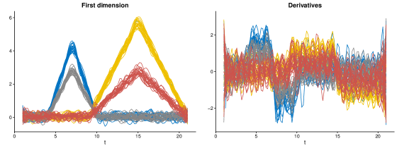
Figure 16: Dimension 1 of DS3 data. Original curves (left panel) and first derivatives (right panel).

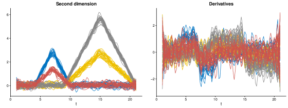
Figure 17: Dimension 2 of DS4 data. Original curves (left panel) and first derivatives (right panel).

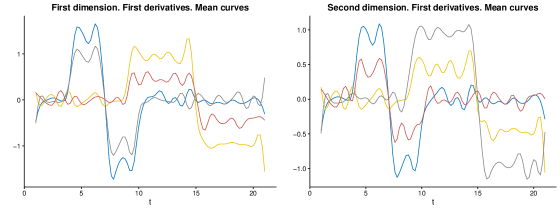
Figure 18: Mean curves of the four groups of DS4 derivatives. Dimension 1 (left panel) and 2 (right panel).

Table 9 presents the outcomes for employing EHyClus to the given dataset. The five highest-ranking outcomes exhibit significantly elevated values for three metrics: Purity (greater than 0.96), F-measure (greater than 0.93), and Rand Index (greater than 0.96). Consequently, EHyClus achieves remarkable precise classification of the dataset. All of these top combinations are attained by simultaneously considering the MEI and MHI and applying k-means with either Euclidean or Mahalanobis distances. The dataset varies in terms of the specific combination of indexes, data, and method utilized. Nevertheless, all five of these combinations involve the inclusion of the original data. Figure 19 depicts the representation of MEI and MHI on the original smoothed curves. This figure clearly demonstrates a distinct separation among the four groups, which can account for the favorable outcomes displayed in Table 9. However, the data considered in the top five results listed in the table comprise combinations of the original data with the first, second, or both derivatives. Due to the complexity of visualizing more than two dimensions, only MEI and MHI over the original curves are depicted here.

Table 9: Top 5 mean results for DS4 with EHyClus on 100 simulations.

	Purity	Fmeasure	RI	Time
kmeans._dd2.MEIMHI-euclidean	0.9684	0.9392	0.9703	0.0080
kmeans._dd2.MEIMHI-mahalanobis	0.9684	0.9392	0.9703	0.0081
kmeans._d.MEIMHI-euclidean	0.9683	0.9390	0.9702	0.0072
kmeans._d.MEIMHI-mahalanobis	0.9683	0.9390	0.9702	0.0074
kmeans._d2.MEIMHI-euclidean	0.9658	0.9346	0.9681	0.0069

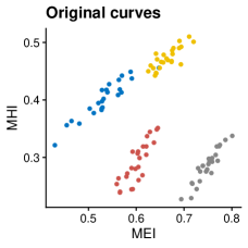
Figure 19: Scatter plot of the modified epigraph index (MEI) and the modified hypograph index (MHI) of the original curves of DS4.

Table 10 represents the mean values obtained over 100 simulations by the six alternative methodologies to whom EHyClus has been compared. EHyClus obtains more than 0.1 unit greater mean values for Purity, F.measure and Rand Index than the top result from this table: funHDDC with 0.8376 purity, 0.8187 F-measure and 0.8886 RI. EHyClus-mean and FGRC are two competitors, obtaining similar values as those achieved with funHDDC. However, they are not competitive to the good outcomes of EHyClus.

Table 10: Mean values for DS4 of Purity, F-measure, Rand Index (RI) and execution time for all the competitors models on 100 simulations.

	Purity	Fmeasure	RI	Time
EHyClus-mean	0.7382	0.6232	0.8142	0.0098
EHyClus-cov	0.5813	0.4528	0.7186	0.0235
Funclust	0.6682	0.6986	0.7908	0.0914
funHDDC	0.8376	0.8187	0.8886	1.4595
FGRC	0.6772	0.6339	0.8163	0.11721
kmeans-d1	0.3962	0.3136	0.6614	0.0261
kmeans-d2	0.4170	0.3350	0.6685	0.03113
gmfd-kmeans	0.7699	0.7389	0.8457	3.8594

Upon analyzing the distribution of the Rand Index for each methodology, as illustrated in 20, it becomes apparent that EHyClus yields the most favorable outcomes, despite its high data variability. The methodology closest to EHyClus in terms of mean metric values, funHDDC, exhibits a less dispersed distribution but clearly inferior results compared to EHyClus. EHyClus-mean and FGRC, although less dispersed, achieve lower values. Furthermore, EHyClus demonstrates that over 50% of its values exceed 0.96, a feat unmatched by any other methodology. Looking at the other methodologies, k-means-d1 and k-means-d2 display some outliers with high RI values; however, their mean results are not satisfactory. Similar behavior is observed with Funclust, which attains both high and low RI values, leading to a lower mean than the one achieved with EHyClus. Overall, EHyClus emerges as the methodology that consistently produces the most accurate results.

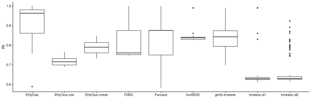
Figure 20: Boxplot of the RI for DS4 over 100 simulation runs of EHyClus and its competitors.

In the combined analysis of DS3 and DS4, it is evident that distinct results arise depending on the model, despite their similar structures. In the case of DS3, FGRC emerges as the superior model, exhibiting a significant performance advantage over the others. Conversely, in DS4, EHyClus takes the lead with a substantial margin compared to the other models. However, it is crucial to acknowledge that both strategies represent two highly effective approaches, with one outperforming the other in each respective case.

5 Applications to real data

In this section, EHyClus for multivariate functional data as proposed in Section 3.1 and tested in different simulated datasets in Section 4, is applied to two real datasets. The first one is the Canadian Weather dataset, highly used in the literature. The second one is a surveillance video data named “WalkByShop1front".

5.1 Canadian Weather data

A popular real dataset in the FDA literature, included in Ramsay  Silverman ³⁷ and in the fda R-package, is the Canadian weather dataset. It contains the daily temperature and precipitation averaged over 1960 to 1994 at 35 different Canadian weather stations grouped into 4 different regions: Artic (3), Atlantic (15), Continental (12) and Pacific (5). The temperature and precipitation curves are represented in Figure 21, and the distribution of the 35 different stations in 4 regions is illustrated by Figure 22.

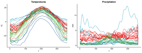
Figure 21: Temperature and precipitation curves of 35 different Canadian weather stations, organized in four different climate zones.

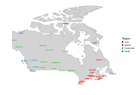
Figure 22: Map of Canada with the name of the stations of four different regions represented with different colors.

In Pulido . ³⁶, EHyClus and some other cluster methodologies for functional data in one dimension were applied to cluster temperatures into four groups. The decision of generating 4 groups is based on the grouping in 4 regions given by the own dataset. This decision is also done in some other works, as Jacques  Preda ²³, which provides a multivariate study in 4 clusters of temperature and precipitation. To do so, as the temperatures and precipitations are in different units, they normalize the data in order to properly work with it. In this paper, the normalization of data is unnecessary due to the utilization of MEI and MHI. These indexes are applied to the curves, and they consider the dimensionality of the data, respecting the units of the various dimensions when doing comparisons to the other curves. Consequently, the resultant values of MEI and MHI for a given curve are in a range between 0 and 1. As a result, the dataset derived from applying these indexes to the original dataset is devoid of dissimilar scales, thereby obviating the need for data normalization.

In Jacques  Preda ²³, as well as in this work, the main objective when clustering this dataset is to obtain a classification of the data mainly based on the climatic regions presented in Figure 22. Note that for clustering, only available information on temperature and precipitation is considered, and no geographical information is used.

Table 11 represents the five top results of EHyClus, in which the best one (RI equal to 0.7849) is achieved when considering MEI and MHI. This good result is obtained with two different combinations of the indexes. The first one is in Table 11 and only considers the first derivatives of the data, while the second one includes all the data available. In this case, it becomes evident that having information about the velocity of temperature and precipitation is crucial for achieving a classification into four distinct groups. Table 12 shows the results of the other methodologies used for clustering. In that table, the best mean RI is obtained by EHyClus-mean, follows to EHyClus-cov. This is a good indicator that EHyClus performs well to cluster multivariate functional data.

Table 11: Top 5 results for Canadian Weather data with EHyClus.

	Purity	Fmeasure	RI	Time
complete.d.MEIMHI-euclidean	0.7714	0.6768	0.7849	0.0002
complete._dd2.MEIMHI-euclidean	0.7714	0.6667	0.7849	0.0002
kkmeans._d2.MEIMHI-polydot	0.7429	0.6667	0.7748	0.0104
complete_d.MEI-euclidean	0.7714	0.6548	0.7714	0.0002
complete_dd2.MEI-euclidean	0.7714	0.6548	0.7714	0.0002

Table 12: Purity, F-measure, Rand Index (RI) and execution time of Canadian Weather data for all the competitors models.

	Purity	Fmeasure	RI	Time
EHyClus-mean	0.7429	0.5776	0.7714	0.0185
EHyClus-cov	0.6857	0.5493	0.7160	0.0137
Funclust	0.4286	0.4168	0.5345	0.0260
funHDDC	0.6571	0.4665	0.6924	0.9262
FGRC	0.6857	0.4892	0.6807	0.3491
kmeans-d1	0.4286	0.2551	0.5681	0.1069
kmeans-d2	0.3530	0.3266	0.6626	0.4424
gmfd-kmeans	0.6286	0.4892	0.6807	0.6524

Finally, the clusters obtained applying EHyClus with the combination of method, data and indexes achieving the higher RI is represented in Figure 23. This combination corresponds to hierarchical clustering with complete linkage and Euclidean distance over the modified epigraph and hypograph indexes of the first derivatives of the data, according to Table 11. The resulting groups share temperature and precipitation behaviors, leading to clusters that have a geographical sense. Moreover, this map respects the distribution in regions given by Figure 22 (ground truth), but differs in the stations that are on the region limits, such us Iqualuit in the Artic region, Pr. Geroge and Kamloops in the Pacific region, and three Atlantic regions: Churchill, Winnipeg and Thunderbay. One can notice that when comparing the classification given in Figure 22 to the result obtained with EHyClus in Figure 23, the two classifications only differ in those stations in the border of the four regions. In the EHyClus classification, the dark blue cluster represents the north side of Canada, close to the Artic ocean. The green one mostly represents the Continental stations, while the red one includes south Continental stations and Atlantic stations. Finally, the light blue group includes stations in the Pacific coast. When comparing these results with those obtained by Funclust, available in Jacques  Preda ²³, one can notice that both strategies reduce the Pacific region compared to the ground truth, while extending the Atlantic region. The main differences between the result obtained with EHyClus, and Funclust, are how they extend the Atlantic region, and how they consider the Pacific one. EHyClus consider all the Atlantic stations together, but also include some Continental regions. However, Funclust include almost all south continental stations together with the Atlantic ones. Moreover, some Atlantic stations are considered in the group with the Continental stations. The other main difference is how they consider the Artic region: in the case of EHyClus, it adds some north continental stations to the group, while omitting Igaluit station, so close to the Atlantic Ocean. On the other hand, Funclust create a group with a single station: Besolute. This station is in the north and have differences to the others. Nevertheless, it has similar characteristics to those stations grouped together by EHyClus, leading to a 5 stations cluster. Thus, the obtained distribution of the stations seems consistent based on the location and climactic behavior of Canada.

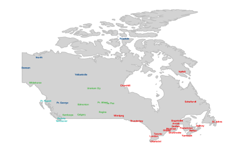
Figure 23: Map of Canada with the names of the stations in four different colors. Each color represents a different cluster obtained with EHyClus.

5.2 Video data

The second real application provided in this work, consists of analyzing data coming from a surveillance video which was made available by CAVIAR: Context Aware Vision using Image-based Active Recognition, funded by the EC’s Information Society Technology’s program project IST 2001 37540 (https://homepages.inf.ed.ac.uk/rbf/CAVIAR/). The video content is the recording of a surveillance camera positioned in front of a clothing store in Lisbon. The video lasts 94 seconds, and includes frames with people as well as frames without people.

This video was previously analyzed in Ojo . ³⁴ and Ojo . ³³. The aim of these works was to identify the presence of outliers, where an outlier was a frame of the video including a person. In this case, we aim to identify two groups in the data: one containing empty frames and the other one including frames with people inside.

The video clip is displayed at a rate of 25 frames per second, with 2359 frames in total. The video has a resolution of 384 $\times$ 288, meaning that each frame consists of 384 $\times$ 288 $=$ 110592 pixels. To represent each frame, the RGB pixel values are organized into an array of size 110592 $\times$ 3. Therefore, we have a trivariate functional dataset with dimensions 2359 $\times$ 110592 $\times$ 3. It contains 2359 functions corresponding to the frames and evaluated at 110592 points that match with the pixels. The three dimensions come from the intensity of the RGB pixels (with three dimensions). Thus, we have obtained a dataset that can be analyzed with clustering techniques for multivariate functional data from a surveillance video. The video contains three big segments in which there are people passing. The first segment contains frames 804–908, where a woman passes in front of the store. The second segment includes frames 1588–2000, during which a man enters the store and two other women pass through it. The third segment contains frames 2073–2359, when another man enters the store. Note that in the frames at the beginning and at the end of these segments, the presence of people is barely discernible. See Figure 24 for two examples, one depicting the initial appearance of a person, and the other representing the presumed final appearance of a person. It is important to emphasize that the presence of the person in these images is nearly imperceptible, and it has been highlighted in red.

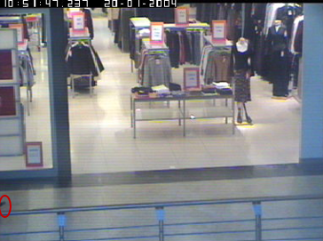
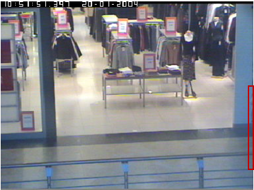
Figure 24: Frame 804 (left) and frame 908 (right). These two frames are the first and the last frames that belong to the ground truth group in which there are some presence of people, although they are classified as having no person. The image portion containing the person is marked in dark red.

analyzing the entire video would necessitate working with a dataset of size 2359 $\times$ 110592 $\times$ 3, which is computationally very demanding. To address this computational burden, a reduction has been employed, specifically targeting the first dimension. Consequently, the number of frames has been decreased, while the time interval and RGB dimensions remain unchanged. For this particular investigation, only the first segment where the woman passes through the store has been considered. In order to preserve the unbalance of the data, the frames 402 to 907 have been considered, leading to a 506 $\times$ 110592 $\times$ 3 dataset which have 79% of empty frames. EHyClus has been applied to this modified dataset and compared against the methodologies explained in Section 3.2, except for FGRC and gmfd-kmeans, as these methodologies are not able to handle the size of this specific dataset.

Table 13 represents the 5 top results obtained when applying EHyClus to the video data. Results obtained in terms of Purity, F-measure and RI are always greater than 0.9, having Purity values up to 0.97 in some cases, which indicates the good performance of EHyClus. Be aware that the time presented in this table does not encompass the duration required to acquire the dataset resulting from the application of the indexes to the data.

Table 13: Top 5 results for Video data with EHyClus.

	Purity	Fmeasure	RI	Time
spc.dd2.MEIMHI	0.9743	0.9634	0.9498	2.7076
svc.dd2.MHI-mlKmeans	0.9723	0.96050	0.9461	0.0115
kkmeans.dd2.MHI-polydot	0.9723	0.9605	0.9461	0.2874
spc.d.MEIMHI	0.9704	0.9581	0.9424	2.9399
svc.d.MEIMHI-kmeans	0.9664	0.9522	0.9349	0.0199

The results obtained by EHyClus, presented in Table 13 are now compared to six different methodologies, two of them with the same approach as EHyClus but with different indexes definitions (see Table 14), with none of these alternatives achieve as good metrics values as EHyClus. Only k-meanss-d1 and funHDDC achieve competitive results, but with values 0.04 and 0.05 units below EHyClus for the three metrics, respectively.

Table 14: Purity, F-measure, Rand Index (RI) and execution time of Video data for all the competitor models.

	Purity	Fmeasure	RI	Time
EHyClus-mean	0.8676	0.8286	0.7698	0.0081
EHyClus-cov	0.6857	0.5493	0.7160	0.0137
Funclust	0.8439	0.8126	0.7360	9.2613
funHDDC	0.9447	0.9258	0.8952	2.7588
kmeans-d1	0.9506	0.9330	0.9059	19.8457
kmeans-d2	0.7925	0.5792	0.5003	19.3927

EHyClus provides accurate results in terms of Purity, F-measure and RI, achieving better results than its competitors. When analyzing the best clustering partition obtained by EHyClus, it distinguishes very well the frames without any person, and the frames with a person in it. Nevertheless, it fails to classify the images where the person starts to appear. Note that in this second case, the ground truth is created after seen the video and manually distinguishing frames where someone appears from those where anyone is passing. All the frames containing a small portion of a person, even if it only includes a little shadow of the person, is included in the group containing people. Table 15 represents the confusion matrix for the best clustering partition obtained with EHyClus. In this case, all the empty frames are classified as so, but some frames classified in the ground truth partition as having some people inside, are misclassified. In particular, seven frames containing a portion of a person at the beginning of the sequence, and six at the end, are misclassified, obtaining 13 misclassified frames in total. Figure 24 shows two frames that EHyClus classifies as containing a person. Looking carefully at these frames, it is difficult to distinguish the small portion of the person appearing in the image. In the first frame, the person starts appearing by the left, while in the second, it is disappearing by the right and only a little shadow can be perceived. Thus, despite that EHyClus misclassifies some frames, it is advisable to consider this kind of people presence as if there are no people, having a really accurate classification into two groups: one with people, and the other one with no people.

Table 15: Confusion matrix obtained from comparing the ground truth (rows) to the classification obtained with EHyClus (columns).

	No people	People inside	Total
No people	401	0	401
People inside	13	92	105
Total	414	92	506

6 Conclusion

The epigraph and hypograph indexes, initially introduced by Franco-Pereira . ¹³, are fundamental tools for analyzing functional data in one dimension. However, extending these indexes to the multivariate context requires careful consideration of the interrelation among the different dimensions of the data. In this study, we address this issue by proposing a novel multivariate definition of these indexes that is not just a combination of the univariate indexes. Previous to this contribution, these indexes have been extended to the multivariate context as a weighted average of the one-dimensional ones.

We present the definitions of the univariate indexes, as well as the alternative extension of the indexes based on the weighted average of the univariate ones. Finally, we present our novel contribution, which provides a comprehensive framework for extending these indexes to the multivariate setting. We also discuss the implications of adopting different definitions and their impact on the ordering of the indexes. Furthermore, we explore the relationship between the multivariate definition and the one-dimensional definitions in each dimension, highlighting that the multivariate indexes are not a linear combination of those in one dimension. Finally, we discuss various theoretical properties associated with the multivariate indexes.

Once the multivariate indexes are defined, we apply them to clustering multivariate functional data. Specifically, we utilize EHyClus, a clustering methodology initially proposed by Pulido . ³⁶ for functional data in one dimension. By leveraging the proposed multivariate definition of the indexes, we extend EHyClus to accommodate multivariate functional data. The necessary code for computing the multivariate indexes and implementing EHyClus can be found in the GitHub repository: https://github.com/bpulidob/EHyClus.

We validate the efficacy of EHyClus by applying it to various simulated and real datasets. Additionally, we compare its performance against other existing approaches in the literature for clustering multivariate functional data. Our results demonstrate the competitiveness of EHyClus in terms of Purity, Rand Index (RI), and F-measure, while also showcasing favorable execution times. However, we acknowledge the need for further improvements in index computation, particularly when dealing with massive datasets. Furthermore, an automatic criterion for selecting the optimal combination of data and indexes in advance, rather than after obtaining all the cluster partitions, would be a valuable enhancement for EHyClus, which will form the base of the future work.

Acknowledgements

This research has been partially supported by Ministerio de Ciencia e Innovación, Gobierno de España, grant numbers PID2019-104901RB-I00, PID2019-104681RB-I00, PTA2020-018802-I, PDC2022-133359 and TED2021-131264B-100 funded by MCIN/AEI/10.13039/501100011033 and European Union NextGenerationEU/PRTR.

Appendix

Proof of Theorem 2.1 for the particular case of $p=3$.

Proof 6.1.

In this particular case,

$$B^{3}_{1,2,3}=\sum_{i=1}^{n}\frac{\lambda(\{x_{i1}\leq x_{1}\}\cap\{x_{i2}\leq x_{2}\}\cap\{x_{i3}\leq x_{3}\})}{n\lambda(I)}.$$

Now, applying the rules of probability,

$$\begin{split}B^{3}_{1,2,3}=&\sum_{i=1}^{n}\frac{\lambda(\{x_{i1}\leq x_{1}\}\cup\{x_{i2}\leq x_{2}\}\cup\{x_{i3}\leq x_{3}\})}{n\lambda(I)}-\sum_{i=1}^{n}\frac{\lambda(x_{i1}\leq x_{1})}{n\lambda(I)}-\sum_{i=1}^{n}\frac{\lambda(x_{i2}\leq x_{2})}{n\lambda(I)}-\sum_{i=1}^{n}\frac{\lambda(x_{i3}\leq x_{3})}{n\lambda(I)}+\\ &\sum_{i=1}^{n}\frac{\lambda(\{x_{i1}\leq x_{1}\}\cap\{x_{i2}\leq x_{2}\})}{n\lambda(I)}+\sum_{i=1}^{n}\frac{\lambda(\{x_{i1}\leq x_{1}\}\cap\{x_{i3}\leq x_{3}\})}{n\lambda(I)}+\sum_{i=1}^{n}\frac{\lambda(\{x_{i2}\leq x_{2}\}\cap\{x_{i3}\leq x_{3}\})}{n\lambda(I)}.\end{split}$$

The expression above can be rewritten in terms of the definition of $B^{3}_{j_{1},\ldots,j_{r}},$ with $\{j_{1},\ldots,j_{r}\}\subseteq\{1,2,3\},$ and $r\leq 3,$ as follows:

$$B^{3}_{1,2,3}=\sum_{i=1}^{n}\frac{\lambda(\{x_{i1}\leq x_{1}\}\cup\{x_{i2}\leq x_{2}\}\cup\{x_{i3}\leq x_{3}\})}{n\lambda(I)}-B^{3}_{1}-B^{3}_{2}-B^{3}_{3}+B^{3}_{1,2}+B^{3}_{1,3}+B^{3}_{2,3}.$$

Taking into account that $\{x_{ij}\leq x_{j}\}^{\mathsf{c}}=\{x_{ij}>x_{j}\},$

$$B^{3}_{1,2,3}=\sum_{i=1}^{n}\frac{\lambda(\{x_{i1}>x_{1}\}^{\mathsf{c}}\cup\{x_{i2}>x_{2}\}^{\mathsf{c}}\cup\{x_{i3}>x_{3}\}^{\mathsf{c}})}{n\lambda(I)}-B^{3}_{1}-B^{3}_{2}-B^{3}_{3}+B^{3}_{1,2}+B^{3}_{1,3}+B^{3}_{2,3}.$$

And applying again the rules of probability,

$$B^{3}_{1,2,3}=\sum_{i=1}^{n}\frac{\lambda(I)-\lambda(\{x_{i1}>x_{1}\}\cap\{x_{i2}>x_{2}\}\cap\{x_{i3}>x_{3}\})}{n\lambda(I)}-B^{3}_{1}-B^{3}_{2}-B^{3}_{3}+B^{3}_{1,2}+B^{3}_{1,3}+B^{3}_{2,3}.$$

Now, taking into consideration that $\{x_{ij}\geq x_{j}\}$ can be written as the union of two disjoint sets as follows:

$$\{x_{ij}\geq x_{j}\}=\{x_{ij}>x_{j}\}\cup\{x_{ij}=x_{j}\}.$$

The following equality holds:

$$\begin{split}\lambda(\{x_{i1}>x_{1}\}\cap\{x_{i2}>x_{2}\ \cap\{x_{i3}>x_{3}\})=&\lambda(\{x_{i1}\geq x_{1}\}\cap\{x_{i2}\geq x_{2}\}\cap\{x_{i3}\geq x_{3}\})-\lambda(\{x_{i1}>x_{1}\}\cap\{x_{i2}=x_{2}\}\cap\{x_{i3}>x_{3}\})-\\ &\lambda(\{x_{i1}=x_{1}\}\cap\{x_{i2}>x_{2}\}\cap\{x_{i3}>x_{3}\})-\lambda(\{x_{i1}=x_{1}\}\cap\{x_{i2}=x_{2}\}\cap\{x_{i3}>x_{3}\})-\\ &\lambda(\{x_{i1}>x_{1}\}\cap\{x_{i2}>x_{2}\}\cap\{x_{i3}=x_{3}\})-\lambda(\{x_{i1}>x_{1}\}\cap\{x_{i2}=x_{2}\}\cap\{x_{i3}=x_{3}\})-\\ &\lambda(\{x_{i1}=x_{1}\}\cap\{x_{i2}>x_{2}\}\cap\{x_{i3}=x_{3}\})-\lambda(\{x_{i1}=x_{1}\}\cap\{x_{i2}=x_{2}\}\cap\{x_{i3}=x_{3}\}).\end{split}$$

Note that the curve $\mathbf{x}$ for which the indexes are calculated is included in the sample. This implies that for any $i=1,...,n$ $x_{ij}=x_{j}$ and as a result $\lambda(\{x_{i1}=x_{1}\}\cap\{x_{i2}=x_{2}\}\cap\{x_{i3}=x_{3}\})=\lambda(I)$. Additionally, for this particular $i$ where $x_{ij}=x_{j}$, it holds that $\{x_{ij}>x_{j}\}=\emptyset$. This leads to the conclusion that all intersections other than the one containing all elements of the form ${x_{ij}=x_{j}}$ are empty sets.

Applying this to $B^{3}_{1,2,3}$, the following expression is obtained:

$$B^{3}_{1,2,3}=-B^{3}_{1}-B^{3}_{2}-B^{3}_{3}+B^{3}_{1,2}+B^{3}_{1,3}+B^{3}_{2,3}+1-A^{3}_{1,2,3}+\frac{1}{n}+R_{3},$$ (18)

where

$$\begin{split}R_{3}=&\sum_{\begin{subarray}{c}i=1\\ x_{i}\neq x\end{subarray}}^{n}\frac{\lambda(\{x_{i1}>x_{1}\}\cap\{x_{i2}=x_{2}\}\cap\{x_{i3}>x_{3}\})}{n\lambda(I)}+\sum_{\begin{subarray}{c}i=1\\ x_{i}\neq x\end{subarray}}^{n}\frac{\lambda(\{x_{i1}=x_{1}\}\cap\{x_{i2}>x_{2}\}\cap\{x_{i3}>x_{3}\})}{n\lambda(I)}+\\ &\sum_{\begin{subarray}{c}i=1\\ x_{i}\neq x\end{subarray}}^{n}\frac{\lambda(\{x_{i1}=x_{1}\}\cap\{x_{i2}=x_{2}\}\cap\{x_{i3}>x_{3}\})}{n\lambda(I)}+\sum_{\begin{subarray}{c}i=1\\ x_{i}\neq x\end{subarray}}^{n}\frac{\lambda(\{x_{i1}>x_{1}\}\cap\{x_{i2}>x_{2}\}\cap\{x_{i3}=x_{3}\})}{n\lambda(I)}+\\ &\sum_{\begin{subarray}{c}i=1\\ x_{i}\neq x\end{subarray}}^{n}\frac{\lambda(\{x_{i1}>x_{1}\}\cap\{x_{i2}=x_{2}\}\cap\{x_{i3}=x_{3}\})}{n\lambda(I)}+\sum_{\begin{subarray}{c}i=1\\ x_{i}\neq x\end{subarray}}^{n}\frac{\lambda(\{x_{i1}=x_{1}\}\cap\{x_{i2}>x_{2}\}\cap\{x_{i3}=x_{3}\})}{n\lambda(I)}+\\ &\sum_{\begin{subarray}{c}i=1\\ x_{i}\neq x\end{subarray}}^{n}\frac{\lambda(\{x_{i1}=x_{1}\}\cap\{x_{i2}=x_{2}\}\cap\{x_{i3}=x_{3}\})}{n\lambda(I)}.\end{split}$$

Thus, applying Equations 14 and 15 to Equation 18:

$$\mathbf{MHI}_{n}(\mathbf{x})-\mathbf{MEI}_{n}(\mathbf{x})=\mathbf{MHI}^{3}_{n,1,2}(\mathbf{x})+\mathbf{MHI}^{3}_{n,1,3}(\mathbf{x})+\mathbf{MHI}^{3}_{n,2,3}(\mathbf{x})-\mathbf{MHI}^{3}_{n,1}(\mathbf{x})-\mathbf{MHI}^{3}_{n,2}(\mathbf{x})-\mathbf{MHI}^{3}_{n,3}(\mathbf{x})+\frac{1}{n}+R_{3}.$$

Proof of Proposition 2.3.

Proof 6.2.

The proof for the epigraph is given here. The one for the hypograph index can be obtained in the same way.

• By definition,

  $$\mathbf{EI}(\mathbf{x})=1-P(\bigcap_{k=1}^{p}\{X_{k}(t)\geq x_{k}(t),t\in\mathcal{I}\}).$$

  Thus, $X_{k}(t)\geq x_{k}(t)$, if and only if, $A_{k}(t)X_{k}(t)\geq A_{k}(t)x_{k}(t)$ and therefore,

  $$\mathbf{EI}(\mathbf{T}(\mathbf{x}))=\mathbf{EI}(\mathbf{x}).$$

• By definition,

  $$\mathbf{EI}(\mathbf{x})=1-P(\bigcap_{k=1}^{p}\{X_{k}(t)\geq x_{k}(t),t\in\mathcal{I}\})$$

  Thus, $X_{k}(t)\geq x_{k}(t)$, if and only if, $X_{k}(g)\geq x_{k}(g)$, as $g$ is a one-to-one transformation of the interval $\mathcal{I}$ $(t\leftrightarrow g)$. Therefore,

  $$\mathbf{EI}(\mathbf{x}(g))=\mathbf{EI}(\mathbf{x}).$$

Proof of Proposition 2.4.

Proof 6.3.

The proof for the epigraph is given here. The one for the hypograph index can be obtained in the same way.

• By definition,

  $$\mathbf{MEI}(\mathbf{x})=1-\sum_{i=1}^{n}\frac{E(\lambda(\bigcap_{k=1}^{p}\{t\in\mathcal{I}:X_{k}(t)\geq x_{k}(t)\}))}{n\lambda(\mathcal{I})}$$

  Thus, $X_{k}(t)\geq x_{k}(t)$, if and only if, $A_{k}(t)X_{k}(t)\geq A_{k}(t)x_{k}(t)$, and therefore,

  $$\mathbf{MEI}(\mathbf{T}(\mathbf{x}))=MEI(\mathbf{x}).$$

• By definition,

  $$\mathbf{MEI}(\mathbf{x})=1-\sum_{i=1}^{n}\frac{E(\lambda(\bigcap_{k=1}^{p}\{t\in\mathcal{I}:X_{k}(t)\geq x_{k}(t)\}))}{n\lambda(\mathcal{I})}$$

  Thus, $X_{k}(t)\geq x_{k}(t)$, if and only if, $X_{k}(g)\geq x_{k}(g)$, as $g$ is a one-to-one transformation of the interval $\mathcal{I}$ $(t\leftrightarrow g)$. Therefore,

  $$\mathbf{MEI}(\mathbf{x}(g))=\mathbf{MEI}(\mathbf{x}).$$

Proof of Proposition 2.5.

Proof 6.4.

To prove this proposition, one needs to prove that

$$\underset{\min_{k=1,...,p}\lVert x_{k}\rVert_{\infty}\geq M}{sup}\mathbf{EI}_{n}(\mathbf{x},P_{\mathbf{X}})\overset{a.s}{\to}1,\ when\ M\to\infty,\ \mathrm{or}$$

$$\underset{\min_{k=1,...,p}\lVert x_{k}\rVert_{\infty}\geq M}{sup}1-\mathbf{HI}_{n}(\mathbf{x},P_{\mathbf{X}})\overset{a.s}{\to}1,\ when\ M\to\infty.$$

Two possibilities arises for $\lVert x_{k}\rVert_{\infty}$:

$$\lVert x_{k}\rVert_{\infty}=sup(x_{k}(t)),\ \mathrm{or}\ \lVert x_{k}\rVert_{\infty}=sup(-x_{k}(t)).$$

When $\lVert x_{k}\rVert_{\infty}=sup(x_{k}(t))$, and $\min_{k=1,...,p}\lVert x_{k}\rVert_{\infty}\geq M$, it happens that the maximum of $x_{k}$ lies in the positive part of the plane. Thus,

$$\underset{min_{k=1,...,p}\lVert x_{k}\rVert_{\infty}\geq M}{sup}\mathbf{EI}_{n}(\mathbf{x})= \underset{min_{k=1,...,p}\lVert x_{k}\rVert_{\infty}\geq M}{sup}1-\frac{1}{n}\sum_{i=1}^{n}I\left(\bigcap_{k=1}^{p}\{x_{ik}(t)\geq x_{k}(t),\ \textit{for all}\ t\in\mathcal{I}\}\right)=$$

$$1-\underset{min_{k=1,...,p}\lVert x_{k}\rVert_{\infty}\geq M}{sup}\frac{1}{n}\sum_{i=1}^{n}I\left(\bigcap_{k=1}^{p}\{x_{ik}(t)\geq x_{k}(t),\ \textit{for all}\ t\in\mathcal{I}\}\right)=$$

$$1-\underset{min_{k=1,...,p}\lVert x_{k}\rVert_{\infty}\geq M}{sup}\frac{1}{n}\sum_{i=1}^{n}\prod_{k=1}^{p}I(\{x_{ik}(t)\geq x_{k}(t),\ \textit{for all}\ t\in\mathcal{I}\})\geq$$

$$1-\underset{min_{k=1,...,p}\lVert x_{k}\rVert_{\infty}\geq M}{sup}\frac{1}{n}\sum_{i=1}^{n}\sum_{k=1}^{p}I(\{x_{ik}(t)\geq x_{k}(t),\ \textit{for all}t\in\mathcal{I}\})\geq$$

$$1-\frac{1}{n}\sum_{i=1}^{n}\sum_{k=1}^{p}\underset{min_{k=1,...,p}\lVert x_{k}\rVert_{\infty}\geq M}{sup}I(\{x_{ik}(t)\geq x_{k}(t),\ \textit{for all}\ t\in\mathcal{I}\})\geq$$

$$1-\frac{1}{n}\sum_{i=1}^{n}\sum_{k=1}^{p}\underset{min_{k=1,...,p}\lVert x_{k}\rVert_{\infty}\geq M}{sup}I(\{\lVert x_{ik}(t)\rVert_{\infty}\geq\lVert x_{k}(t)\rVert_{\infty},\ \textit{for all}\ t\in\mathcal{I}\})\geq$$

$$1-\frac{1}{n}\sum_{i=1}^{n}\sum_{k=1}^{p}I(\{\lVert x_{ik}(t)\rVert_{\infty}\geq M,\ \textit{for all}\ t\in\mathcal{I}\})$$

When $\lVert x_{k}\rVert_{\infty}=sup(-x_{k}(t))$, and $\min_{k=1,...,p}\lVert x_{k}\rVert_{\infty}\geq M$, it happens that the minimum of $x_{k}$ lies in the negative part of the plane. Thus,

$$\underset{min_{k=1,...,p}\lVert x_{k}\rVert_{\infty}\geq M}{sup}1-\mathbf{HI}_{n}(\mathbf{x})= \underset{min_{k=1,...,p}\lVert x_{k}\rVert_{\infty}\geq M}{sup}1-\frac{1}{n}\sum_{i=1}^{n}I\left(\bigcap_{k=1}^{p}\{x_{ik}(t)\leq x_{k}(t),\ \textit{for all}\ t\in\mathcal{I}\}\right)=$$

$$\underset{min_{k=1,...,p}\lVert x_{k}\rVert_{\infty}\geq M}{sup}1-\frac{1}{n}\sum_{i=1}^{n}I\left(\bigcap_{k=1}^{p}\{-x_{ik}(t)\geq-x_{k}(t),\ \textit{for all}\ t\in\mathcal{I}\}\right)=$$

$$1-\underset{min_{k=1,...,p}\lVert x_{k}\rVert_{\infty}\geq M}{sup}\frac{1}{n}\sum_{i=1}^{n}I\left(\bigcap_{k=1}^{p}\{-x_{ik}(t)\geq-x_{k}(t),\ \textit{for all}\ t\in\mathcal{I}\}\right)=$$

$$1-\underset{min_{k=1,...,p}\lVert x_{k}\rVert_{\infty}\geq M}{sup}\frac{1}{n}\sum_{i=1}^{n}\prod_{k=1}^{p}I(\{-x_{ik}(t)\geq-x_{k}(t),\ \textit{for all}\ t\in\mathcal{I}\})\geq$$

$$1-\underset{min_{k=1,...,p}\lVert x_{k}\rVert_{\infty}\geq M}{sup}\frac{1}{n}\sum_{i=1}^{n}\sum_{k=1}^{p}I(\{-x_{ik}(t)\geq-x_{k}(t),\ \textit{for all}\ t\in\mathcal{I}\})\geq$$

$$1-\frac{1}{n}\sum_{i=1}^{n}\sum_{k=1}^{p}\underset{min_{k=1,...,p}\lVert x_{k}\rVert_{\infty}\geq M}{sup}I(\{-x_{ik}(t)\geq-x_{k}(t),\ \textit{for all}\ t\in\mathcal{I}\})\geq$$

$$1-\frac{1}{n}\sum_{i=1}^{n}\sum_{k=1}^{p}\underset{min_{k=1,...,p}\lVert x_{k}\rVert_{\infty}\geq M}{sup}I(\{\lVert-x_{ik}(t)\rVert_{\infty}\geq\lVert-x_{k}(t)\rVert_{\infty},\ \textit{for all}\ t\in\mathcal{I}\})\geq$$

$$1-\frac{1}{n}\sum_{i=1}^{n}\sum_{k=1}^{p}I(\{\lVert-x_{ik}(t)\rVert_{\infty}\geq M,\ \textit{for all}\ t\in\mathcal{I}\})$$

It is sufficient to prove that $I(\{\lVert x_{ik}(t)\rVert_{\infty}\geq M,\ \textit{for all}\ t\in\mathcal{I}\}\overset{a.s}{\to}0,\ when\ M\to\infty$, or equivalently that
$P(\underset{M\geq l}{sup}I\{\lVert x_{ik}(t)\rVert_{\infty}\geq M,\ \textit{for all}\ t\in\mathcal{I}\}>\epsilon)\to 0\ when\ M\to\infty.$

The following inequality is satisfied:

$$\underset{M\geq l}{sup}I\{\lVert x_{ik}(t)\rVert_{\infty}\geq M,\ \textit{for all}\ t\}\leq I\{\lVert x_{ik}(t)\rVert_{\infty}\geq l,\ \textit{for all}\ t\in\mathcal{I}\}.$$

And it implies that,

$$P(\underset{M\geq l}{sup}\ I\{\lVert x_{ik}(t)\rVert_{\infty}\geq M,\ \textit{for all}\ t\in\mathcal{I}\}>\epsilon)\leq P(I\{\lVert x_{ik}(t)\rVert_{\infty}\geq l,\ \textit{for all}\ t\in\mathcal{I}\}>\epsilon)=P(\lVert x_{ik}(t)\rVert_{\infty}\geq l,\ \textit{for all}\ t\in\mathcal{I})\to 0,\ when\ l\to\infty.$$

Thus, regardless of where the supremum of $x_{k}$ is achieved,

$$\underset{\min_{k=1,...,p}\lVert x_{k}\rVert_{\infty}\geq M}{sup}\max\{\mathbf{EI}_{n}(\mathbf{x},P_{\mathbf{X}}),1-\mathbf{HI}_{n}(\mathbf{x},P_{\mathbf{X}})\}\overset{a.s}{\to}1,\ when\ M\to\infty,$$

References

- Abraham \BOthers. \APACyear2003 \APACinsertmetastarabraham2003{APACrefauthors}Abraham, C., Cornillon, P\BHBIA., Matzner-Løber, E.\BCBL \BBA Molinari, N. \APACrefYearMonthDay2003. \BBOQ\APACrefatitleUnsupervised curve clustering using B-splines Unsupervised curve clustering using b-splines.\BBCQ \APACjournalVolNumPagesScandinavian journal of statistics303581–595. \PrintBackRefs\CurrentBib
- Arribas-Gil \BBA Romo \APACyear2014 \APACinsertmetastararribas{APACrefauthors}Arribas-Gil, A.\BCBT \BBA Romo, J. \APACrefYearMonthDay2014. \BBOQ\APACrefatitleShape outlier detection and visualization for functional data: the outliergram Shape outlier detection and visualization for functional data: the outliergram.\BBCQ \APACjournalVolNumPagesBiostatistics154603–619. \PrintBackRefs\CurrentBib
- Ben-Hur \BOthers. \APACyear2001 \APACinsertmetastarsvc{APACrefauthors}Ben-Hur, A., Horn, D., Siegelmann, H\BPBIT.\BCBL \BBA Vapnik, V. \APACrefYearMonthDay2001. \BBOQ\APACrefatitleSupport vector clustering Support vector clustering.\BBCQ \APACjournalVolNumPagesJournal of machine learning research2Dec125–137. \PrintBackRefs\CurrentBib
- Blanquero \BOthers. \APACyear2019 \APACinsertmetastarblanquero2019{APACrefauthors}Blanquero, R., Carrizosa, E., Jiménez-Cordero, A.\BCBL \BBA Martín-Barragán, B. \APACrefYearMonthDay2019. \BBOQ\APACrefatitleVariable selection in classification for multivariate functional data Variable selection in classification for multivariate functional data.\BBCQ \APACjournalVolNumPagesInformation Sciences481445–462. \PrintBackRefs\CurrentBib
- Boullé \APACyear2012 \APACinsertmetastarboulle{APACrefauthors}Boullé, M. \APACrefYearMonthDay2012. \BBOQ\APACrefatitleFunctional data clustering via piecewise constant nonparametric density estimation Functional data clustering via piecewise constant nonparametric density estimation.\BBCQ \APACjournalVolNumPagesPattern Recognition45124389–4401. \PrintBackRefs\CurrentBib
- Bouveyron \BOthers. \APACyear2015 \APACinsertmetastarBouveyron2015{APACrefauthors}Bouveyron, C., Côme, E.\BCBL \BBA Jacques, J. \APACrefYearMonthDay2015. \BBOQ\APACrefatitleTHE DISCRIMINATIVE FUNCTIONAL MIXTURE MODEL FOR A COMPARATIVE ANALYSIS OF BIKE SHARING SYSTEMS The discriminative functional mixture model for a comparative analysis of bike sharing systems.\BBCQ \APACjournalVolNumPagesThe Annals of Applied Statistics941726–1760. \PrintBackRefs\CurrentBib
- Chiou \BBA Li \APACyear2007 \APACinsertmetastarchiou2007functional{APACrefauthors}Chiou, J\BHBIM.\BCBT \BBA Li, P\BHBIL. \APACrefYearMonthDay2007. \BBOQ\APACrefatitleFunctional clustering and identifying substructures of longitudinal data Functional clustering and identifying substructures of longitudinal data.\BBCQ \APACjournalVolNumPagesJournal of the Royal Statistical Society Series B: Statistical Methodology694679–699. \PrintBackRefs\CurrentBib
- Dai \BBA Genton \APACyear2018\APACexlab\BCnt1 \APACinsertmetastardai2018{APACrefauthors}Dai, W.\BCBT \BBA Genton, M\BPBIG. \APACrefYearMonthDay2018\BCnt1. \BBOQ\APACrefatitleFunctional boxplots for multivariate curves Functional boxplots for multivariate curves.\BBCQ \APACjournalVolNumPagesStat71e190. \PrintBackRefs\CurrentBib
- Dai \BBA Genton \APACyear2018\APACexlab\BCnt2 \APACinsertmetastardai2018multivariate{APACrefauthors}Dai, W.\BCBT \BBA Genton, M\BPBIG. \APACrefYearMonthDay2018\BCnt2. \BBOQ\APACrefatitleMultivariate functional data visualization and outlier detection Multivariate functional data visualization and outlier detection.\BBCQ \APACjournalVolNumPagesJournal of Computational and Graphical Statistics274923–934. \PrintBackRefs\CurrentBib
- Dhillon \BOthers. \APACyear2004 \APACinsertmetastarkkmenas{APACrefauthors}Dhillon, I\BPBIS., Guan, Y.\BCBL \BBA Kulis, B. \APACrefYearMonthDay2004. \BBOQ\APACrefatitleKernel k-means: spectral clustering and normalized cuts Kernel k-means: spectral clustering and normalized cuts.\BBCQ \BIn \APACrefbtitleProceedings of the tenth ACM SIGKDD international conference on Knowledge discovery and data mining Proceedings of the tenth acm sigkdd international conference on knowledge discovery and data mining (\BPGS 551–556). \PrintBackRefs\CurrentBib
- Ferraty \BBA Vieu \APACyear2006 \APACinsertmetastarferraty{APACrefauthors}Ferraty, F.\BCBT \BBA Vieu, P. \APACrefYear2006. \APACrefbtitleNonparametric functional data analysis: theory and practice Nonparametric functional data analysis: theory and practice. \APACaddressPublisherSpringer Science & Business Media. \PrintBackRefs\CurrentBib
- Franco-Pereira \BBA Lillo \APACyear2020 \APACinsertmetastarfranc2020{APACrefauthors}Franco-Pereira, A\BPBIM.\BCBT \BBA Lillo, R\BPBIE. \APACrefYearMonthDay2020. \BBOQ\APACrefatitleRank tests for functional data based on the epigraph, the hypograph and associated graphical representations Rank tests for functional data based on the epigraph, the hypograph and associated graphical representations.\BBCQ \APACjournalVolNumPagesAdvances in Data Analysis and Classification143651–676. {APACrefDOI} 10.1007/s11634-019-00380-9 \PrintBackRefs\CurrentBib
- Franco-Pereira \BOthers. \APACyear2011 \APACinsertmetastarfranc2011{APACrefauthors}Franco-Pereira, A\BPBIM., Lillo, R\BPBIE.\BCBL \BBA Romo, J. \APACrefYearMonthDay2011. \BBOQ\APACrefatitleExtremality for functional data Extremality for functional data.\BBCQ \BIn F. Ferraty (\BED), \APACrefbtitleRecent advances in functional data analysis and related topics Recent advances in functional data analysis and related topics (\BVOL 14, \BPG 651-676). \APACaddressPublisherSpringer, New York. \PrintBackRefs\CurrentBib
- Giacofci \BOthers. \APACyear2013 \APACinsertmetastargiacofci2013wavelet{APACrefauthors}Giacofci, M., Lambert-Lacroix, S., Marot, G.\BCBL \BBA Picard, F. \APACrefYearMonthDay2013. \BBOQ\APACrefatitleWavelet-based clustering for mixed-effects functional models in high dimension Wavelet-based clustering for mixed-effects functional models in high dimension.\BBCQ \APACjournalVolNumPagesBiometrics69131–40. \PrintBackRefs\CurrentBib
- Horváth \BBA Kokoszka \APACyear2012 \APACinsertmetastarhorvath{APACrefauthors}Horváth, L.\BCBT \BBA Kokoszka, P. \APACrefYear2012. \APACrefbtitleInference for functional data with applications Inference for functional data with applications (\BVOL 200). \APACaddressPublisherSpringer Science & Business Media. \PrintBackRefs\CurrentBib
- Hsing \BBA Eubank \APACyear2015 \APACinsertmetastarhsing{APACrefauthors}Hsing, T.\BCBT \BBA Eubank, R. \APACrefYear2015. \APACrefbtitleTheoretical foundations of functional data analysis, with an introduction to linear operators Theoretical foundations of functional data analysis, with an introduction to linear operators (\BVOL 997). \APACaddressPublisherJohn Wiley & Sons. \PrintBackRefs\CurrentBib
- Ieva \BBA Paganoni \APACyear2013 \APACinsertmetastarieva2013depth{APACrefauthors}Ieva, F.\BCBT \BBA Paganoni, A\BPBIM. \APACrefYearMonthDay2013. \BBOQ\APACrefatitleDepth measures for multivariate functional data Depth measures for multivariate functional data.\BBCQ \APACjournalVolNumPagesCommunications in Statistics-Theory and Methods4271265–1276. \PrintBackRefs\CurrentBib
- Ieva \BBA Paganoni \APACyear2020 \APACinsertmetastarieva2020component{APACrefauthors}Ieva, F.\BCBT \BBA Paganoni, A\BPBIM. \APACrefYearMonthDay2020. \BBOQ\APACrefatitleComponent-wise outlier detection methods for robustifying multivariate functional samples Component-wise outlier detection methods for robustifying multivariate functional samples.\BBCQ \APACjournalVolNumPagesStatistical Papers612595–614. \PrintBackRefs\CurrentBib
- Ieva \BOthers. \APACyear2013 \APACinsertmetastarieva2011{APACrefauthors}Ieva, F., Paganoni, A\BPBIM., Pigoli, D.\BCBL \BBA Vitelli, V. \APACrefYearMonthDay2013. \BBOQ\APACrefatitleMultivariate functional clustering for the analysis of ECG curves morphology Multivariate functional clustering for the analysis of ecg curves morphology.\BBCQ \APACjournalVolNumPagesJournal of the Royal Statistical Society Series C623401–418. \PrintBackRefs\CurrentBib
- Ieva \BOthers. \APACyear2019 \APACinsertmetastarieva2019roahd{APACrefauthors}Ieva, F., Paganoni, A\BPBIM., Romo, J.\BCBL \BBA Tarabelloni, N. \APACrefYearMonthDay2019. \BBOQ\APACrefatitleroahd Package: Robust Analysis of High Dimensional Data roahd Package: Robust Analysis of High Dimensional Data.\BBCQ \APACjournalVolNumPagesThe R Journal112291–307. {APACrefURL} https://doi.org/10.32614/RJ-2019-032 {APACrefDOI} 10.32614/RJ-2019-032 \PrintBackRefs\CurrentBib
- Jacques \BBA Preda \APACyear2013 \APACinsertmetastarjacques2013{APACrefauthors}Jacques, J.\BCBT \BBA Preda, C. \APACrefYearMonthDay2013. \BBOQ\APACrefatitleFunclust: A curves clustering method using functional random variables density approximation Funclust: A curves clustering method using functional random variables density approximation.\BBCQ \APACjournalVolNumPagesNeurocomputing112164–171. \PrintBackRefs\CurrentBib
- Jacques \BBA Preda \APACyear2014\APACexlab\BCnt1 \APACinsertmetastarjacques2014S{APACrefauthors}Jacques, J.\BCBT \BBA Preda, C. \APACrefYearMonthDay2014\BCnt1. \BBOQ\APACrefatitleFunctional data clustering: a survey Functional data clustering: a survey.\BBCQ \APACjournalVolNumPagesAdvances in Data Analysis and Classification83231–255. \PrintBackRefs\CurrentBib
- Jacques \BBA Preda \APACyear2014\APACexlab\BCnt2 \APACinsertmetastarjacques2014{APACrefauthors}Jacques, J.\BCBT \BBA Preda, C. \APACrefYearMonthDay2014\BCnt2. \BBOQ\APACrefatitleModel-based clustering for multivariate functional data Model-based clustering for multivariate functional data.\BBCQ \APACjournalVolNumPagesComputational Statistics & Data Analysis7192–106. \PrintBackRefs\CurrentBib
- Jain \APACyear2010 \APACinsertmetastarkmeans{APACrefauthors}Jain, A\BPBIK. \APACrefYearMonthDay2010. \BBOQ\APACrefatitleData clustering: 50 years beyond K-means Data clustering: 50 years beyond k-means.\BBCQ \APACjournalVolNumPagesPattern recognition letters318651–666. \PrintBackRefs\CurrentBib
- James \BBA Sugar \APACyear2003 \APACinsertmetastarjames2003{APACrefauthors}James, G\BPBIM.\BCBT \BBA Sugar, C\BPBIA. \APACrefYearMonthDay2003. \BBOQ\APACrefatitleClustering for sparsely sampled functional data Clustering for sparsely sampled functional data.\BBCQ \APACjournalVolNumPagesJournal of the American Statistical Association98462397–408. \PrintBackRefs\CurrentBib
- Kayano \BOthers. \APACyear2010 \APACinsertmetastarkayano2010{APACrefauthors}Kayano, M., Dozono, K.\BCBL \BBA Konishi, S. \APACrefYearMonthDay2010. \BBOQ\APACrefatitleFunctional cluster analysis via orthonormalized Gaussian basis expansions and its application Functional cluster analysis via orthonormalized gaussian basis expansions and its application.\BBCQ \APACjournalVolNumPagesJournal of Classification272211–230. \PrintBackRefs\CurrentBib
- López-Pintado \BOthers. \APACyear2014 \APACinsertmetastarlop2014{APACrefauthors}López-Pintado, S., Sun, Y., Lin, J\BPBIK.\BCBL \BBA Genton, M\BPBIG. \APACrefYearMonthDay2014. \BBOQ\APACrefatitleSimplicial band depth for multivariate functional data Simplicial band depth for multivariate functional data.\BBCQ \APACjournalVolNumPagesAdvances in Data Analysis and Classification83321–338. \PrintBackRefs\CurrentBib
- López-Pintado \BBA Romo \APACyear2011 \APACinsertmetastarlop2011{APACrefauthors}López-Pintado, S.\BCBT \BBA Romo, J. \APACrefYearMonthDay2011. \BBOQ\APACrefatitleA half-region depth for functional data A half-region depth for functional data.\BBCQ \APACjournalVolNumPagesComputational Statistics and Data Analysis551679-1695. \PrintBackRefs\CurrentBib
- Manning \BOthers. \APACyear2009 \APACinsertmetastarindexes{APACrefauthors}Manning, C\BPBID., Raghavan, P.\BCBL \BBA Schüte, H. \APACrefYear2009. \APACrefbtitleIntroduction to information retrieval Introduction to information retrieval. \APACaddressPublisherCambridge, UP. \PrintBackRefs\CurrentBib
- Martin-Barragan \BOthers. \APACyear2016 \APACinsertmetastarmartin2016{APACrefauthors}Martin-Barragan, B., Lillo, R.\BCBL \BBA Romo, J. \APACrefYearMonthDay2016. \BBOQ\APACrefatitleFunctional boxplots based on epigraphs and hypographs Functional boxplots based on epigraphs and hypographs.\BBCQ \APACjournalVolNumPagesJournal of Applied Statistics4361088–1103. \PrintBackRefs\CurrentBib
- Martino \BOthers. \APACyear2019 \APACinsertmetastarmartino{APACrefauthors}Martino, A., Ghiglietti, A., Ieva, F.\BCBL \BBA Paganoni, A\BPBIM. \APACrefYearMonthDay2019. \BBOQ\APACrefatitleA k-means procedure based on a Mahalanobis type distance for clustering multivariate functional data A k-means procedure based on a mahalanobis type distance for clustering multivariate functional data.\BBCQ \APACjournalVolNumPagesStatistical Methods & Applications282301–322. \PrintBackRefs\CurrentBib
- Murtagh \BBA Contreras \APACyear2012 \APACinsertmetastarhierarc{APACrefauthors}Murtagh, F.\BCBT \BBA Contreras, P. \APACrefYearMonthDay2012. \BBOQ\APACrefatitleAlgorithms for hierarchical clustering: an overview Algorithms for hierarchical clustering: an overview.\BBCQ \APACjournalVolNumPagesWiley Interdisciplinary Reviews: Data Mining and Knowledge Discovery2186–97. \PrintBackRefs\CurrentBib
- Ojo \BOthers. \APACyear2023 \APACinsertmetastarojo2023{APACrefauthors}Ojo, O\BPBIT., Fernández Anta, A., Genton, M\BPBIG.\BCBL \BBA Lillo, R\BPBIE. \APACrefYearMonthDay2023. \BBOQ\APACrefatitleMultivariate functional outlier detection using the fast massive unsupervised outlier detection indices Multivariate functional outlier detection using the fast massive unsupervised outlier detection indices.\BBCQ \APACjournalVolNumPagesStat121e567. \PrintBackRefs\CurrentBib
- Ojo \BOthers. \APACyear2022 \APACinsertmetastarojo2022{APACrefauthors}Ojo, O\BPBIT., Fernández Anta, A., Lillo, R\BPBIE.\BCBL \BBA Sguera, C. \APACrefYearMonthDay2022. \BBOQ\APACrefatitleDetecting and classifying outliers in big functional data Detecting and classifying outliers in big functional data.\BBCQ \APACjournalVolNumPagesAdvances in Data Analysis and Classification163725–760. \PrintBackRefs\CurrentBib
- Peng \BOthers. \APACyear2008 \APACinsertmetastarpeng2008{APACrefauthors}Peng, J., Müller, H\BHBIG.\BCBL \BOthersPeriod. \APACrefYearMonthDay2008. \BBOQ\APACrefatitleDistance-based clustering of sparsely observed stochastic processes, with applications to online auctions Distance-based clustering of sparsely observed stochastic processes, with applications to online auctions.\BBCQ \APACjournalVolNumPagesAnnals of Applied Statistics231056–1077. \PrintBackRefs\CurrentBib
- Pulido \BOthers. \APACyear2023 \APACinsertmetastarpulido2023{APACrefauthors}Pulido, B., Franco-Pereira, A\BPBIM.\BCBL \BBA Lillo, R\BPBIE. \APACrefYearMonthDay2023. \BBOQ\APACrefatitleA fast epigraph and hypograph-based approach for clustering functional data A fast epigraph and hypograph-based approach for clustering functional data.\BBCQ \APACjournalVolNumPagesStatistics and Computing33236. \PrintBackRefs\CurrentBib
- Ramsay \BBA Silverman \APACyear2005 \APACinsertmetastarramsay{APACrefauthors}Ramsay, J\BPBIO.\BCBT \BBA Silverman, B\BPBIW. \APACrefYear2005. \APACrefbtitleFunctional Data Analysis Functional data analysis (\PrintOrdinal2 \BEd). \APACaddressPublisherSpringer. \PrintBackRefs\CurrentBib
- Rendón \BOthers. \APACyear2011 \APACinsertmetastarrendon{APACrefauthors}Rendón, E., Abundez, I., Arizmendi, A.\BCBL \BBA Quiroz, E\BPBIM. \APACrefYearMonthDay2011. \BBOQ\APACrefatitleInternal versus external cluster validation indexes Internal versus external cluster validation indexes.\BBCQ \APACjournalVolNumPagesInternational Journal of computers and communications5127–34. \PrintBackRefs\CurrentBib
- Rossi \BOthers. \APACyear2004 \APACinsertmetastarrossi2004{APACrefauthors}Rossi, F., Conan-Guez, B.\BCBL \BBA El Golli, A. \APACrefYearMonthDay2004. \BBOQ\APACrefatitleClustering functional data with the SOM algorithm. Clustering functional data with the som algorithm.\BBCQ \BIn \APACrefbtitleESANN Esann (\BPGS 305–312). \PrintBackRefs\CurrentBib
- Schmutz \BOthers. \APACyear2020 \APACinsertmetastarschmutz2020{APACrefauthors}Schmutz, A., Jacques, J., Bouveyron, C., Cheze, L.\BCBL \BBA Martin, P. \APACrefYearMonthDay2020. \BBOQ\APACrefatitleClustering multivariate functional data in group-specific functional subspaces Clustering multivariate functional data in group-specific functional subspaces.\BBCQ \APACjournalVolNumPagesComputational Statistics3531101–1131. \PrintBackRefs\CurrentBib
- Song \BBA Kim \APACyear2022 \APACinsertmetastarsong2022{APACrefauthors}Song, J.\BCBT \BBA Kim, K. \APACrefYearMonthDay2022. \BBOQ\APACrefatitleSparse multivariate functional principal component analysis Sparse multivariate functional principal component analysis.\BBCQ \APACjournalVolNumPagesStat111e435. \PrintBackRefs\CurrentBib
- Tarpey \BBA Kinateder \APACyear2003 \APACinsertmetastartarpey2003{APACrefauthors}Tarpey, T.\BCBT \BBA Kinateder, K\BPBIK. \APACrefYearMonthDay2003. \BBOQ\APACrefatitleClustering Functional Data. Clustering functional data.\BBCQ \APACjournalVolNumPagesJournal of classification20122–93. \PrintBackRefs\CurrentBib
- Traore \BOthers. \APACyear2019 \APACinsertmetastartraore2019{APACrefauthors}Traore, O., Cristini, P., Favretto-Cristini, N., Pantera, L., Vieu, P.\BCBL \BBA Viguier-Pla, S. \APACrefYearMonthDay2019. \BBOQ\APACrefatitleClustering acoustic emission signals by mixing two stages dimension reduction and nonparametric approaches Clustering acoustic emission signals by mixing two stages dimension reduction and nonparametric approaches.\BBCQ \APACjournalVolNumPagesComputational Statistics342631–652. \PrintBackRefs\CurrentBib
- Von Luxburg \APACyear2007 \APACinsertmetastarspc{APACrefauthors}Von Luxburg, U. \APACrefYearMonthDay2007. \BBOQ\APACrefatitleA tutorial on spectral clustering A tutorial on spectral clustering.\BBCQ \APACjournalVolNumPagesStatistics and computing17395–416. \PrintBackRefs\CurrentBib
- Wang \BOthers. \APACyear2016 \APACinsertmetastarwang{APACrefauthors}Wang, J\BHBIL., Chiou, J\BHBIM.\BCBL \BBA Müller, H\BHBIG. \APACrefYearMonthDay2016. \BBOQ\APACrefatitleFunctional data analysis Functional data analysis.\BBCQ \APACjournalVolNumPagesAnnual Review of Statistics and Its Application3257–295. \PrintBackRefs\CurrentBib
- Yamamoto \BBA Hwang \APACyear2017 \APACinsertmetastaryamamoto2017{APACrefauthors}Yamamoto, M.\BCBT \BBA Hwang, H. \APACrefYearMonthDay2017. \BBOQ\APACrefatitleDimension-reduced clustering of functional data via subspace separation Dimension-reduced clustering of functional data via subspace separation.\BBCQ \APACjournalVolNumPagesJournal of Classification34294–326. \PrintBackRefs\CurrentBib
- Zeng \BOthers. \APACyear2019 \APACinsertmetastarzeng2019simultaneous{APACrefauthors}Zeng, P., Qing Shi, J.\BCBL \BBA Kim, W\BHBIS. \APACrefYearMonthDay2019. \BBOQ\APACrefatitleSimultaneous registration and clustering for multidimensional functional data Simultaneous registration and clustering for multidimensional functional data.\BBCQ \APACjournalVolNumPagesJournal of Computational and Graphical Statistics284943–953. \PrintBackRefs\CurrentBib