An Empirical Study on Log-based Anomaly Detection Using Machine Learning

Abstract

The growth of systems complexity increases the need of automated techniques dedicated to different log analysis tasks such as Log-based Anomaly Detection (LAD). The latter has been widely addressed in the literature, mostly by means of different deep learning techniques. Nevertheless, the focus on deep learning techniques results in less attention being paid to traditional Machine Learning (ML) techniques, which may perform well in many cases, depending on the context and the used datasets. Further, the evaluation of different ML techniques is mostly based on the assessment of their detection accuracy. However, this is is not enough to decide whether or not a specific ML technique is suitable to address the LAD problem. Other aspects to consider include the training and prediction time as well as the sensitivity to hyperparameter tuning.

In this paper, we present a comprehensive empirical study, in which we evaluate different supervised and semi-supervised, traditional and deep ML techniques w.r.t. four evaluation criteria: detection accuracy, time performance, sensitivity of detection accuracy as well as time performance to hyperparameter tuning.

The experimental results show that supervised traditional and deep ML techniques perform very closely in terms of their detection accuracy and prediction time. Moreover, the overall evaluation of the sensitivity of the detection accuracy of the different ML techniques to hyperparameter tuning shows that supervised traditional ML techniques are less sensitive to hyperparameter tuning than deep learning techniques. Further, semi-supervised techniques yield significantly worse detection accuracy than supervised techniques.

I Introduction

Systems typically produce execution logs recording execution information about the state of the system, inputs and outputs, and operations performed. These logs are typically used during testing campaigns, to detect failures, or after deployment and at runtime, to identify abnormal system behaviors; these are referred to as anomalies.

The Log-based Anomaly Detection (LAD) problem consists of detecting anomalies from execution logs recording normal and abnormal system behaviors. It has been widely addressed in the literature by means of deep learning techniques [1, 2, 3, 4, 5, 6, 7, 8, 9, 10, 11, 12, 13, 14]. Since logs are typically unstructured, all LAD techniques (with the exception of NeuraLog [11]) rely on log parsing (e.g., using Drain [15]) to identify and extract log templates (also called log events). The extracted templates can be grouped into different windows (i.e., fixed, sliding, or session windows) forming different template sequences.

Features first need to be extracted from different template sequences to enable the use of machine learning (ML) techniques. DeepLog [1], for example, extracts features using sequential vectors where each dimension in a vector is an index-based encoding of a single template within a template sequence. The remaining deep learning techniques rely on semantic vectors to capture the semantic information from the different templates within a sequence. Semantic vectors are obtained by means of different semantic vectorization techniques such as Template2Vec [6], word2vec augmented by Post-Processing Algorithm (PPA) [10], FastText [8] or a transformer-based encoder [4, 12, 11]. Existing deep learning techniques detect log anomalies using RNN [1, 2, 3, 5, 6, 7, 8, 13], CNN [9, 10, 14] and Transformer-based deep learning models [4, 11, 12].

Some empirical studies [11, 16] investigate the impact of log parsing methods on the detection accuracy of deep learning anomaly detection techniques. Others [17] study the impact of different semantic vectorization techniques on the detection accuracy of deep learning techniques.

Detection accuracy has also been further evaluated to assess the impact of several factors [16], such as training data selection strategies, data grouping methods, data imbalance and data noise (e.g., log mislabelling). A high detection accuracy of a technique may, however, come with a time performance cost (training and prediction), and hence, might not be a recommended option from a practical standpoint. Some empirical studies, e.g., [4, 7, 10, 11] assess the time performance of alternative LAD techniques. Further, a technique with a high detection accuracy and a practical time performance, when evaluated with a particular hyperparameter setting and dataset, still can yield widely different results with other settings and datasets.

For the aforementioned reasons, we contend that four evaluation criteria should be systemically considered to assess the overall performance of any ML technique for LAD, regardless of the type of learning. These criteria are i) detection accuracy, ii) time performance, sensitivity of iii) detection accuracy and iv) time performance to different hyperparameter settings across datasets.

Most of the aforementioned empirical studies focus on deep learning techniques. Although a few studies [4, 8, 11, 12] compare some deep learning techniques to traditional ones, none of these studies systematically evaluates the technique they propose and the alternative ML techniques w.r.t. the four aforementioned evaluation criteria. Including semi-supervised learning in such studies is also important given the usual scarcity of anomalies in many logs.

In this study, we perform the first comprehensive, systematic empirical study that includes not only deep learning techniques but also traditional ones, both supervised and semi-supervised, considering the four aforementioned evaluation criteria. More precisely, we systematically evaluate and compare, on two benchmark datasets (HDFS and Hadoop), a) supervised traditional (SVM [18] and Random Forest [19]) and deep learning techniques (LSTM [20] and LogRobust [8]), as well as b) semi-supervised traditional (OC-SVM [21]) and deep learning techniques (DeepLog [1]) in terms of i) detection accuracy, ii) time performance, sensitivity of iii) detection accuracy and iv) time performance to hyperparameter tuning.

Our experimental results show that supervised traditional and deep ML techniques perform very closely in terms of detection accuracy and prediction time. Further, supervised traditional ML techniques show less sensitivity to hyperparameter tuning than deep learning techniques. Semi-supervised, traditional and deep learning techniques, however, do not fare well, in terms of detection accuracy, when compared to supervised ones. The results suggest that, despite the focus on research on deep learning solutions for LAD, traditional ML techniques such as Random Forest can fare much better with respect to our four criteria and therefore be a solution of choice in practice.

Paper structure. The paper is organized as follows. Section II explains and formalizes the background concepts used in the rest of the paper and provides a brief overview of the ML techniques considered in the study. Section III reports on state-of-the-art empirical studies that are related to the study presented in the paper. Section IV explains the semantic vector embedding techniques we used to extract features from the input data. Section V describes the design of our empirical study. Section VI reports on evaluation results of the different supervised and semi-supervised ML techniques. Section VII discusses the practical implications of our study and its threats to validity. Section VIII concludes the paper, providing directions for future work.

II Background

In this section, we first introduce the different concepts used in the remainder of the paper (§ II-A). We then briefly illustrate three traditional ML techniques (§ II-B) and three deep learning techniques (§ II-C) that have been previously used to address the LAD problem and further considered in our study.

II-A Execution Logs

Information about system executions is usually stored in log files, called execution logs. These logs help with troubleshooting and hence help system engineers understand the behavior of the system under analysis across its different executions. We distinguish between normal and abnormal system executions. The former represents an expected behavior of the system, while the latter represents an anomalous system behavior, possibly leading to a failure. These system executions are therefore stored in labeled execution logs, where the label refers to whether the execution is normal or not.

An execution log can be defined as a sequence of consecutive log entries that represent the behavior of the system over a given time period. A log entry contains: i) an ID, ii) the timestamp at which the logged event was recorded; iii) the log message denoting the occurrence of an event, also called log event occurrence and iv) the parameter value(s) recorded for that specific log event occurrence. Figure 1 shows an example of log containing ten log entries (seven of which are displayed in the figure). For instance, the log entry with ID=4 in the figure contains the timestamp “16:05:14”, an occurrence of log event gyroscope_sensor, and the corresponding parameter values ($0.0012$, $-0.0086$ and $0.0020$). The different log entries collected in a log are chronologically ordered w.r.t. their recorded timestamps.

ID	Timestamp	Log Event Occurrence	Parameter Value
$1$	$16:05:12$	$battery\_filtered\_voltage$	$16.182$
$2$	$16:05:13$	$gyroscope\_sensor$	$-0.0013$, $-1.135$, $-0.002$
$3$	$16:05:13$	$ekf2\_attitude\_pitch$	$-0.026$
$4$	$16:05:14$	$gyroscope\_sensor$	$0.0012$, $-0.0086$, $0.0020$
$5$	$16:05:14$	$battery\_filtered\_voltage$	$15.687$
$6$	$16:05:19$	$battery\_filtered\_voltage$	$14.921$
$\dots$	$\dots$	$\dots$	…
$10$	$16:05:48$	$ekf2\_attitude\_pitch$	$-0.025$

Figure 1: Example of an Execution Log

An execution path is the projection with respect to the log event occurrences of the sequence of log entries recorded in the log. For instance, let us consider the first three log entries in Figure 1. The execution path obtained from these entries is the sequence of the three corresponding log event occurrences (battery_filtered_voltage, gyroscope_sensor, ekf2_attitude_pitch). An execution path is called anomalous (i.e., containing execution path log anomalies) when the order of its sequence of log event occurrences is unexpected.

Given a log $\sigma$, we denote by $\sigma(l)$ the log event occurrence recorded at the entry of log $\sigma$ having an ID equal to $l$. For instance, given the log in Figure 1, we have $\sigma(2)=\text{{gyroscope\_sensor}}$. We introduce a word-based tokenization function $W$ that, given a log event occurrence as input, returns the sequence of words contained in the log event occurrence. For instance, $W(\sigma(2))=(\text{{gyroscope}},\text{{sensor}})$.

II-B Traditional ML Techniques

We briefly describe three traditional ML techniques further used in this study: SVM [18], Random Forest [19], and OC-SVM [21]. We selected these techniques since they have been used as alternatives in the evaluation of previous work on LAD [4, 8, 11, 5, 12].

II-B1 Support Vector Machine (SVM)

SVM is a supervised classification ML technique. The key component of SVM is the kernel function, which significantly affects classification accuracy. The Radial Basis kernel Function (RBF) is typically the default choice when the problem requires a non-linear model (i.e., non-linearly separable data). SVM is based on a hyperparameter $\gamma$ that controls the distance of influence of a single training data point and a regularization hyperparameter $C$ that is used to add penalty to misclassified data points. SVM was used as an alternative supervised traditional ML technique in the evaluation of some of the SOTA LAD techniques [4, 8, 11]. The experiments of LogRobust[8] and NeuraLog[11] show good detection accuracy of SVM, when evaluated on HDFS— one of the datasets we consider in this empirical study (see Section V-B).

II-B2 Random Forest (RF)

RF is a supervised classification ML technique. Two main hyperparameters can impact its accuracy: the number of decision trees $\mathit{dTr}$ (a user-specific hyperparameter that depends of data dimensionality) and the number of randomly selected features $\mathit{sFeat}$ used in each node of a decision tree. RF is used as a supervised traditional ML technique in the evaluation of one of the LAD techniques [5] and showed a better detection accuracy than other techniques.

II-B3 One-class SVM (OC-SVM)

OC-SVM is a semi-supervised classification ML technique. It has the same hyperparameters as SVM. Anomaly detection using OC-SVM requires building a feature matrix from the normal input. Unlike the unbounded SVM hyperparameter $C$, the regularization hyperparameter $\nu$ of OC-SVM is lower bounded by the fraction of support vectors (i.e., minimum percentage of data points that can act as support vectors). OC-SVM is a variant of SVM, which was also used as a semi-supervised alternative technique in the evaluation of LogBert [12].

II-C Log-based Deep Learning Techniques

Over the years, there have been several proposals to use deep learning for LAD [1, 6, 8, 9, 7, 4, 11, 12, 10, 22].

Many of the semi-supervised and supervised deep learning techniques in the literature rely on Recurrent Neural Network (RNN), i.e., [1, 6, 8, 2, 5, 13]). More specifically, these techniques are based on LSTM, initially introduced in [20]. In the following, we briefly illustrate three deep learning techniques (LSTM [20], DeepLog [1] and LogRobust [8]) that rely on RNN-based detection models and that we use in this study. We selected these three techniques among others since they are commonly used in the LAD literature [6, 2, 5, 13, 4, 10, 11, 16] and they have shown promising results in terms of detection accuracy.

II-C1 LSTM [20]

LSTM is a supervised deep learning technique. It is known for its capability to learn long-term dependencies between different sequence inputs. LSTM is mainly defined with the following hyperparameters: i) a loss function $\mathit{lF}$; ii) an optimizer $\mathit{opt}$; iii) a number of hidden layers $\mathit{hL}$; iv) a number of memory units in a single LSTM block $\mathit{mU}$; and v) a number of epochs $\mathit{epN}$.

II-C2 DeepLog [1]

Deeplog is a semi-supervised technique. It relies on a forecasting-based detection model i.e., anomalies are detected by predicting the next log event given preceding log events. DeepLog has been used as an alternative technique in many past studies [2, 3, 4, 5, 6, 7, 13, 10, 12, 14, 16].

II-C3 LogRobust [8]

LogRobust is a supervised technique. It relies on a classification-based detection model, i.e., anomalies are detected by classifying anomalous log event sequences. It has been frequently used in past studies [4, 10, 11, 13, 16] and showed a high detection accuracy.

III State of the Art

An in-depth analysis of representative semi-supervised (DeepLog [1] and LogAnomaly [6]) and supervised (LogRobust [8], PleLog [7] and CNN [9]) deep learning techniques was conducted in a recent study [16], in which several model evaluation criteria (i.e., training data selection strategy, log data grouping, early detection ability, imbalanced class distribution, quality of data and early detection ability) were considered to assess the detection accuracy of these different techniques. The study concludes that the detection accuracy of the five deep learning LAD techniques, when taking into account the aforementioned evaluation criteria, is lower than the one reported in the original papers. For instance, the training data strategies significantly impact the detection accuracy of semi-supervised deep learning techniques. Further, data noise such as mislabelled logs (e.g., logs with errors resulting from the domain expert labelling process) heavily impacts the detection accuracy of supervised deep learning techniques.

Reference [16] also shows that the comparison of the detection accuracy of supervised LAD techniques to semi-supervised ones depends on the evaluation criteria considered. On the one hand, although the semi-supervised techniques DeepLog [1] and LogAnomaly [6] are sensitive to training data strategies, they are less sensitive to mislabeled logs than the supervised techniques. On the other hand, supervised deep learning techniques show better detection accuracy than semi-supervised ones when evaluated on a large amount of data (e.g., log event sequences), in spite of their sensitivity to mislabeled logs.

Although many deep learning techniques for LAD showed a high detection accuracy ([1, 6, 8, 4, 11]), some of them may not perform well, in terms of training time or prediction time, when compared to traditional ML techniques. For instance, NeuraLog [11] and HitAnomaly [4] are slower than traditional ML techniques in terms of their training and prediction time, respectively. Moreover, traditional ML techniques can be more suitable to detect log anomalies, depending on their application domain and the used datasets. For instance, when datasets are small, traditional ML techniques can be a good option to detect log anomalies as they are known to be less data hungry than deep learning-ones. Nevertheless, traditional ML techniques can also be sensitive w.r.t. their detection accuracy or time performance, to hyperparameter tuning and different datasets.

Further, a ML technique with a high detection accuracy and reasonable time performance, when evaluated on a particular hyperparameter setting and dataset still can show a low detection accuracy and impractical time performance, when evaluated with other hyperparameter settings and datasets.

We therefore contend that four evaluation criteria should be systemically considered to assess the overall performance of any ML technique, regardless of the type of learning. These criteria are i) detection accuracy, ii) time performance, sensitivity of iii) detection accuracy and iv) time performance w.r.t. different hyperparameter settings across datasets.

In Table I, we summarize the evaluation strategies of 14 deep learning techniques for LAD techniques, including the five techniques considered in the aforementioned work [16]. Column C.L indicates, using the symbols N and Y, whether the proposed deep learning anomaly detection technique was compared to at least one traditional ML technique that shares the same model learning type, i.e., whether the deep learning and the traditional ML techniques put in comparison are both supervised or semi-supervised. We also indicate, for each work, whether the evaluation considered: the detection accuracy (column Acc.), the time performance (column Time), the sensitivity of the detection accuracy to hyperparameter tuning and different datasets (columns S.H and S.D, respectively, under the Sensitivity/Acc. column), as well as the sensitivity of the time performance to hyperparameter tuning across datasets (columns S.H and S.D under the Sensitivity/Time column). For each of these criteria, we use symbol $+$ to indicate if the evaluation criterion is considered for all the techniques used in the experiments; symbol $\pm$ indicates that the evaluation criterion is only computed for the main technique; symbol $-$ indicates that the evaluation criterion is not measured for any of the techniques considered in the paper.

TABLE I: Comparison Of the Evaluation Strategies Of Deep Learning Log-based Anomaly Detection Approaches

Technique	C.L	Acc.	Time	Sensitivity
				Acc.		Time
				S.H	S.D	S.H	S.D
DeepLog [1]	N	+	$\pm$	$\pm$	-	-	-
LogNL [2]	N	+	-	$\pm$	-	-	-
Att-Gru [3]	N	+	$\pm$	-	-	-	-
HitAnomaly [4]	Y	+	+	$\pm$	-	-	-
LogNads [5]	Y	+	$\pm$	-	-	-	-
LogAnomaly [6]	N	+	-	-	-	-	-
PleLog [7]	N	+	+	$\pm$	$\pm$	-	-
LogRobust [8]	Y	+	-	-	-	-	-
CNN [9]	N	+	-	+	-	-	-
LightLog [10]	N	+	+	-	-	-	-
NeuralLog [11]	Y	+	+	$\pm$	$\pm$	-	-
logBert [12]	Y	+	-	$\pm$	-	-	-
LogEncoder [13]	N	+	-	$\pm$	-	-	-
EdgeLog [14]	N	+	$\pm$	-	-	-	-

As shown in Table I, all the existing empirical studies report the detection accuracy of all the techniques considered in the study. Only a few existing empirical studies — focusing on supervised [4, 5, 8, 11] and semi-supervised [12] approaches — compare, in terms of detection accuracy, the proposed technique with (at least) a traditional ML technique that shares the same model learning type.

However, none of these studies provides a systematic evaluation of all the techniques considered in their experimental campaign w.r.t. all the evaluation criteria discussed above, i.e., i) the detection accuracy, ii) the time performance, sensitivity of iii) the detection accuracy and iv) the time performance to hyperparameter tuning across datasets.

Given the aforementioned limitations of existing empirical studies, in this paper we report on the first, comprehensive empirical study, in which we not only evaluate the detection accuracy of existing supervised and semi-supervised, traditional and deep learning techniques applied to the detection of execution path log anomalies, but also assess their time performance as well as the sensitivity of their detection accuracy and their time performance to hyperparameter tuning across datasets.

IV Log Representation

Sequences of log event occurrences are mainly textual. To be fed to proper ML techniques, these sequences need to be first converted into numerical representations that are understandable by such techniques, while preserving their original meaning (e.g., the different words forming each log event occurrence, the relationship between the different log event occurrences forming these sequences).

To encode sequences of log event occurrences, we apply an encoding technique that relies on FastText [23], a semantic vectorization technique used by some previous LAD studies [8, 16]. Specifically, we use the same log encoding technique adopted by LogRobust [8]. We first pre-process sequences of log event occurrences (e.g., removing non-character tokens, splitting composite tokens into individual ones). We then apply a three-step encoding technique (i.e., word-vectorization, log event occurrence vectorization, sequence vectorization), which we describe in the following.

Word Vectorization

FastText [23] vectorization technique maps each word $w_{i},1\leq i\leq E$, in the sequence of words $W(\sigma(l))=(w_{1},w_{2},\dots,w_{E})$ extracted from the log event occurrence $\sigma(l)$, to a $d$-dimensional word vector $v_{o}$ where $1\leq o\leq E$ and $d=300$.

For instance, let us consider the log event occurrences battery_filtered_voltage and gyroscope_ sensor, recorded in the first two log entries in Figure 1. The corresponding lists of words are $W(\sigma(1))=(\mathit{battery},\mathit{filtered},\mathit{voltage})$ and $W(\sigma(2))=(\mathit{gyroscope},\mathit{sensor})$. By setting the word vector dimension to $d=2$, the different word vectors resulting from FastText and associated to the words $\mathit{battery}$, $\mathit{filtered}$, $\mathit{voltage}$, $\mathit{gyroscope}$, and $\mathit{sensor}$ are $v_{1}=[-0.2759,-0.0023]$, $v_{2}=[0.2618,0.1413]$, $v_{3}=[-0.4211,0.4043]$, $v_{4}=[0.3276,0.4368]$ and $v_{5}=[-0.3419,0.4418]$, respectively.

Log Event Occurrence Vectorization

We transform the word list $W(\sigma(l))$ into a word vector list $\mathit{WV}(\sigma(l))$, such that $\mathit{WV}(\sigma(l))=[v_{1},v_{2},\dots,v_{E}]$, where $v_{j}\in\mathbb{R}^{d}$ and $j\in[1,E]$ denotes the word vector. $\mathit{WV}(\sigma(l))$ is finally transformed to an aggregated word vector by aggregating all its word vectors using the weighted aggregation technique TF-IDF [24], i.e., a technique that measures the importance of the different words defined in a log event occurrence within a log. For instance, the word vector lists associated to the word lists $W(\sigma(1))$ and $W(\sigma(2))$ are $\mathit{WV}(\sigma(1))=[[-0.2759,-0.0023],[0.2618,0.1413],[-0.4211,0.4043]]$ and $\mathit{WV}(\sigma(2))=[[0.3276,0.4368],[-0.3419,0.4418]]$, respectively. The corresponding aggregated word vectors obtained by means of TF-IDF are $[-0.2038,0.2545]$ and $[-0.0100,0.6174]$, respectively.

Sequence Vectorization

Given the aggregated word vectors from the previous step, the latter are further aggregated to form a sequence vector, i.e., a representation of the sequence of log event occurrences. More in details, the aggregation is done by means of the average operator for each dimension of the aggregated word vectors. For example, if we consider the sequence of log event occurrences obtained from the first two log entries in Figure 1, given the corresponding aggregated word vectors from the previous step ($[-0.2038,0.2545]$ and $[-0.0100,0.6174]$), the final sequence vector is $[-0.1069,0.4359]$.

V Empirical Study Design

V-A Research Questions

The goal of our study is to evaluate alternative ML techniques (described in Section II) when applied to the detection of execution path log anomalies, considering both supervised and semi-supervised, traditional and deep learning techniques. The evaluation is performed based on the four evaluation criteria described in Section III. We address the following research questions:

RQ1

How do supervised traditional ML techniques compare to supervised deep learning ones at detecting execution path log anomalies?

RQ2

How do semi-supervised traditional ML techniques compare to semi-supervised deep learning ones at detecting execution path log anomalies?

These research questions are motivated by the fact that traditional ML techniques are less data hungry than deep learning ones, and are therefore more practical in many contexts. Therefore, if the loss in detection accuracy is acceptable, assuming there is any, such techniques are preferable. Similarly, given the scarcity of anomalies in many logs, semi-supervised techniques should be considered in certain contexts.

V-B Benchmark Datasets

Most of existing techniques in Table I have been evaluated on public benchmark datasets, published in the LogHub dataset collection [25], such as HDFS [26] and BGL [27]. Different synthesized versions of the original HDFS dataset have been also proposed in the context of the empirical evaluation of LogRobust [8] and HitAnomaly [4]; these versions have been obtained by removing, inserting, or shuffling log events within log event sequences. OpenStack [1] is also a synthesized dataset that was used to evaluate DeepLog [1], LogNL [2] and HitAnomaly [4]. In addition to the HDFS and OpenStack datasets, an industrial one from Microsoft (not publicly available due to confidentiality reasons) was also used to evaluate LogRobust [8]. EdgeLog [14] was evaluated on HDFS, BGL and OpenStack, as well as Hadoop [28]. In this empirical study, we are interested in evaluating different ML techniques on datasets that are i) suitable for detecting execution path log anomalies (i.e., datasets containing sequences of log messages), ii) labeled and iii) grouped into sessions (representing full system executions). Among the datasets mentioned above, only HDFS, Hadoop, and OpenStack satisfy the above requirements. OpenStack, however, is too imbalanced (i.e., anomalies are only injected in four out of 2069 sequences of log event occurrences) and is, hence, not suitable for our experiments. We therefore evaluate the different ML techniques at detecting execution path log anomalies on the HDFS and Hadoop datasets, which we describe in the following.

HDFS

The Hadoop Distributed File System (HDFS) dataset was produced from more than 200 nodes of the Amazon EC2 web service. HDFS contains 11,175,629 log messages collected from 575,061 different labeled blocks representing 558,223 normal and 16,838 anomalous program executions.

Hadoop

Hadoop contains logs collected from a computing cluster running two MapReduce jobs (WordCount and PageRank). Different types of failures (e.g., machine shut-down, network disconnection, full hard disk) were injected in the logs. The dataset contains 978 executions; 167 logs are normal and the remaining ones (811 logs) are abnormal.

Table II describes the two aforementioned benchmark datasets used in our experiments (column Dataset). Columns #N and #A under #Seq indicate the total number of normal and anomalous log event sequences, respectively. Columns Min and Max under #Len denote the minimum and the maximum sequence length, respectively.

TABLE II: Characteristics of Benchmark Datasets

Dataset	#Seq		#Len
	#N	#A	Min	Max
HDFS	558223	16838	1	297
Hadoop	167	811	5	11846

V-C Evaluation Metrics

We evaluate the detection accuracy of the alternative ML techniques using common evaluation metrics: precision, recall and F1-score. We first define standard concepts based on the confusion matrix:

• TP (True Positive) is the number of the abnormal sequences of log event occurrences that are correctly detected by the model.

• FP (False Positive) is the number of normal sequences of log event occurrences that are wrongly identified as anomalies by the model.

• TN (True Negative) are normal sequences of log event occurrences that are classified correctly.

• FN (False Negative) is the number of abnormal sequences of log event occurrences that are not detected by the model.

We therefore define the three evaluation metrics as follows. Precision is the percentage of the correctly detected anomalous sequences of log event occurrences over all the anomalous sequences detected by the model; the corresponding formula is $\mathit{Prec}=\frac{\mathit{TP}}{\mathit{TP}+\mathit{FP}}$. Recall is the percentage of sequences of log event occurrences that are correctly identified as anomalous over all real anomalous sequences in the dataset; it is defined as: $\mathit{Rec}=\frac{\mathit{TP}}{\mathit{TP}+\mathit{FN}}$. The F1-score represents the harmonic mean of precision and recall: $\mathit{F1}=\frac{2*\mathit{Prec}*\mathit{Rec}}{\mathit{Prec}+\mathit{Rec}}$.

V-D Experimental Setup

In this empirical study, as discussed in Section II, we consider six alternative ML techniques. Three of them are traditional, i.e., SVM, RF and OC-SVM (see Section II-B). The three remaining ones are deep learning-based, i.e., DeepLog[1], LogRobust [8] and LSTM [20] (see Section II-C).

V-D1 Hyperparameter Settings

Each of the six alternative ML techniques considered in our study has hyperparameters that first need to be tuned before models can be trained. In the following, we provide different hyperparameter settings associated with each of the techniques considered in this study.

• SVM [18]. We used the RBF kernel function, set the values of $\mathit{C}$ to 1, 10, 100 and 1000, and took the values of $\gamma$ from the set {0.0001, 0.001, 0.01, 0.1}, leading to 16 different hyperparameter settings (i.e., combinations of hyperparameter values).

• RF [19]. We set the number of decision trees $\mathit{dTr}$ to values ranging from 10 to 100 in steps of 10, and set the number of features $\mathit{sFeat}$ in a single node of each decision tree to the square root of the total number of features (i.e., the total features represent the 300 dimensions of the encoded sequence of log event occurrences (see Section IV)), leading to 10 hyperparameter settings.

• OC-SVM [21]. We used the RBF kernel function, set the values of $\nu$ ranging from 0.1 to 0.9 in steps of 0.1, and — similarly to the SVM settings — we took the values of $\gamma$ from the set {0.0001, 0.001, 0.01, 0.1}, leading to 36 different hyperparameter settings.

• LSTM, LogRobust and DeepLog. To train the three deep learning-based techniques (LSTM [20], LogRobust [8] and DeepLog [1]), we set the loss function $\mathit{lF}$ to the binary cross entropy, the optimizer $\mathit{opt}$ to the three commonly used optimizers (adam, rmsprop, and adadelta), the number of hidden layers $\mathit{hL}$ to 2, the memory units $\mathit{mU}$ to three different values (32, 64 and 128) and the number of epochs $\mathit{epN}$ from the set {10, 50, 100, 150}, leading to 36 different hyperparameter settings for each of these techniques.

V-D2 Hyperparameter Tuning

Table III summarizes the strategy we followed to divide the benchmark datasets to enable training. Symbol $C_{1}$ denotes the majority class in each dataset, whereas $C_{2}$ denotes the minority class. Column Learning indicates the learning type, semi-supervised or supervised . We divided each dataset used in our experiments into training, validation, and testing sets and assigned different proportions for these sets depending on the learning type of each technique as follows:

• Semi-supervised. Models are trained on 70% of the majority class, validated on 10% of each class and tested on the remaining set (10% $C_{1}$ and 90% $C_{2}$).

• Supervised. Models are trained on 70% of each class, validated on 10% of each class, and tested on the remaining set (20% $C_{1}$ and 20% $C_{2}$).

For each learning algorithm, we carried out hyperparameter tuning, using a grid search [30]. For each hyperparameter setting, we trained the ML technique on the training set and validated it on the validation set. To avoid biased results and assess the stability of the detection accuracy of each technique, we repeated this process (training and validation) five times, computed precision, recall, and F1-score, and recorded the computational time needed for the training phase (training time and validation time) for each iteration; we report the average values from the five iterations.

Collecting the average F1-score for each hyperparameter setting of a ML technique, when evaluated on each dataset, allows us to study the sensitivity of detection accuracy for that technique. Similarly, collecting the average computational time needed for the training phase for each hyperparameter setting serves to assess the sensitivity of time performance of each of the ML techniques used in this study, considering each dataset separately.

Given that there are 16, 10 and 36 hyperparameter settings for traditional techniques (SVM, RF and OC-SVM) and 36 hyperparameter settings for each of the three deep learning techniques (LSTM, DeepLog and LogRobust), the total number of hyperparameter settings considered in this study during hyperparameter tuning is 170. Running each algorithm five times for a single hyperparameter setting and repeating the process for two datasets leads to $170\times 5\times 2=1700$ executions of all the algorithms.

We selected the best hyperparameter setting for each algorithm w.r.t the best F1-score. We used the best hyperparameter setting to re-train the model on the training and validation sets and evaluated it on the test set. We repeated the process five times, computed the precision, recall, F1-score, re-train time, recording the test time per iteration; we report the corresponding average values from the five iterations.

The average F1-score for the best hyperparameter setting associated with each ML technique, evaluated on each dataset, is meant to reflect the best possible detection accuracy of that technique. Similarly, collecting the average re-train time and test time for the best hyperparameter setting reflects the overall time performance of each ML technique.

Each of the six algorithms is executed five times for the best hyperparameter setting for each of the two datasets used in our study, leading to a total number of $6\times 5\times 2=60$ executions.

TABLE III: Set up of benchmark datasets

Learning	Training	Validation	Test
Semi-supervised	70% $C_{1}$	10% $C_{1}$ 10% $C_{2}$	20% $C_{1}$ 90% $C_{2}$
Supervised	70% $C_{1}$ 70% $C_{2}$	10% $C_{1}$ 10% $C_{2}$	20% $C_{1}$ 20% $C_{2}$

$C_{1}$ ($C_{2}$) is the the majority (minority) class in each dataset

VI Results

In this section, we first report the hyperparameter settings that led to the best detection accuracy (highest F1-score) for each ML technique used to answer RQ1 and RQ2. Then, for each research question, we report the detection accuracy and the time performance (i.e., re-training and prediction time) associated with the best hyperparameter setting, and discuss the sensitivity of detection accuracy and time performance (training time) of each ML technique w.r.t. hyperparameter tuning across datasets. We finally discuss and compare the obtained results across techniques.

VI-A Best hyperparameter settings for RQ1 and RQ2

Table IV shows the hyperparameter settings that led to the best detection accuracy of each ML technique used to answer RQ1 and RQ2.

TABLE IV: Best Hyperparameter Setting

Technique	Hyperparameter settings
	HDFS	Hadoop
SVM	$C=1000$ $\gamma=0.1$	$\mathit{C}=1000$ $\gamma=0.0001$
RF	$\mathit{dTr}=100$	$\mathit{dTr}=50$
LSTM	$\mathit{opt}=\texttt{adam}$ $\mathit{epN}=100$ $\mathit{mU}=32$	$\mathit{opt}=\texttt{adam}$ $\mathit{epN}=100$ $\mathit{mU}=32$
LogRobust	$\mathit{opt}=\texttt{rmsprop}$ $\mathit{epN}=10$ $\mathit{mU}=32$	$\mathit{opt}=\texttt{rmsprop}$ $\mathit{epN}=150$ $\mathit{mU}=128$
OC-SVM	$\nu=0.1$ $\gamma=0.01$	$\nu=0.4$ $\gamma=0.1$
DeepLog	$\mathit{opt}=\texttt{adadelta}$ $\mathit{epN}=10$ $\mathit{mU}=128$	$\mathit{opt}=\texttt{rmsprop}$ $\mathit{epN}=100$ $\mathit{mU}=64$

VI-B RQ1 Results

To answer RQ1, we evaluated the performance of the traditional and deep ML techniques at detecting execution path log anomalies on the HDFS and Hadoop datasets.

Detection Accuracy

As shown in Table V, both supervised traditional (SVM, RF) and deep (LSTM, LogRobust) learning techniques show a high detection accuracy (in terms of F1-score) when evaluated on both datasets, with better results on HDFS than Hadoop.

TABLE V: Comparison of the detection accuracy of supervised traditional and deep ML techniques on HDFS and Hadoop datasets

Dataset	Metric	Technique
		SVM	RF	LSTM	LogRobust
HDFS	Prec	93.61	93.68	93.60	99.78
	Rec	100.00	99.97	99.17	99.04
	F1	96.70	96.73	96.30	99.41
Hadoop	Prec	82.74	83.35	83.49	82.74
	Rec	100.00	97.06	99.26	100.00
	F1	90.56	89.68	90.69	90.56

The overall detection accuracy of both supervised traditional and deep learning techniques on both datasets is very similar. There are no significant differences and therefore accuracy is not a distinguishing factor among techniques. The difference between the highest detection accuracy of traditional techniques (96.73 for RF) and the highest detection accuracy of deep learning techniques (99.41 for LogRobust) on HDFS is small (2.68). Similarly, the difference between the highest detection accuracy of traditional techniques (90.56 for SVM) and the highest detection accuracy of deep learning techniques (90.69 for LSTM) on Hadoop is also small (0.13).

Time Performance

In Table VI, we report the model re-training time and the prediction time (Columns Re-train. and Test., respectively) for the supervised traditional and deep ML techniques on HDFS and Hadoop datasets. One important result is that the overall model re-training time of traditional ML techniques is about an order of magnitude shorter than that of deep learning techniques, on both datasets. The prediction time computed for all the supervised traditional and deep learning techniques is similar, on both datasets, with no practical differences. Therefore prediction time is not a distinguishing factor among techniques.

TABLE VI: Time performance (in seconds) of supervised traditional and supervised deep ML techniques on HDFS and Hadoop datasets

Technique	Dataset
	HDFS		Hadoop
	Re-train.	Test.	Re-train.	Test.
SVM	149.56	7.49	0.04	0.01
RF	164.63	1.50	0.27	0.01
LSTM	2922.72	3.09	7.46	0.35
LogRobust	1523	3.56	2.21	0.01

Sensitivity of Detection Accuracy

As depicted in Figure 2, sensitivity analysis to hyperparameter tuning in terms of detection accuracy across datasets shows that deep learning techniques lead to much more sensitivity than traditional techniques on both HDFS (left box plot) and Hadoop (right box plot) datasets.

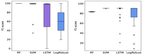
Figure 2: Sensitivity of the detection accuracy of supervised traditional and deep learning techniques on HDFS (left) and Hadoop (right) datasets.

More in detail, on HDFS, the detection accuracy of LSTM ranges from $0.0$ to $99.58$ (avg $\approx 81.72$, StdDev $\approx 27.52$) and that of LogRobust ranges from $19.51$ to $99.87$ (avg $\approx 62.49$, StdDev $\approx 21.39$), thus showing very large sensitivity in terms of F1-score. SVM yields a couple of outliers but has otherwise very low sensitivity. RF is, however, the least sensitive technique to hyperparameter tuning with very low sensitivity and no outliers: its detection accuracy ranges from $99.77$ to $99.82$ (avg $\approx 99.80$, StdDev $\approx 0.02$). On Hadoop, LogRobust is the most sensitive technique to hyperparameter tuning, with an F1-score ranging from $8.46$ to $90.50$ (avg $\approx 76.65$, StdDev $\approx 24.23$). LSTM is less sensitive to hyperparameter tuning than LogRobust, showing an F1-score that ranges from $20.79$ to $90.60$ (avg $\approx 87.03$, StdDev $\approx 11.70$), whereas SVM and RF are significantly less sensitive to hyperparameter tuning than both deep learning techniques. The F1-score of RF on Hadoop ranges from $82.54$ to $83.94$ (avg $\approx 83.37$, StdDev $\approx 0.41$), whereas the detection accuracy of SVM is the least sensitive to hyperparameter tuning, showing an F1-score that ranges from $89.77$ to $90.50$ (avg $\approx 90.46$, StdDev $\approx 0.18$).

Sensitivity of Training Time

As depicted in Figure 3, on HDFS (left box plot), the training time of RF is significantly less sensitive to hyperparameter tuning than the one of the remaining techniques. RF takes from $14.02\text{\,}\mathrm{s}$ to $133.00\text{\,}\mathrm{s}$ to train the model (avg $\approx$74.25\text{\,}\mathrm{s}$$, stdDev $\approx$38.22\text{\,}\mathrm{s}$$). The training time of SVM is the most sensitive to hyperparameter tuning compared to the remaining techniques. Its model training ranges from $69.69\text{\,}\mathrm{s}$ to $25\,990.41\text{\,}\mathrm{s}$ (avg $\approx$9254.99\text{\,}\mathrm{s}$$, stdDev $\approx$8758.88\text{\,}\mathrm{s}$$).

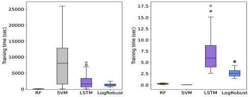
Figure 3: Sensitivity of training time of supervised traditional and deep learning techniques on HDFS (left) and Hadoop (right) datasets.

Regarding deep learning techniques, the training time of LogRobust is less sensitive to hyperparameter tuning than that of LSTM. Its model training ranges from $633.29\text{\,}\mathrm{s}$ to $2463.83\text{\,}\mathrm{s}$ (avg $\approx$1387.77\text{\,}\mathrm{s}$$, stdDev $\approx$536.34\text{\,}\mathrm{s}$$) whereas LSTM takes from $68.69\text{\,}\mathrm{s}$ to $8362.02\text{\,}\mathrm{s}$ (avg $\approx$2330.36\text{\,}\mathrm{s}$$, stdDev $\approx$2099.56\text{\,}\mathrm{s}$$) for the corresponding model training across the different hyperparameter settings. The lower sensitivity of LogRobust, in terms of its model training time, to hyperparameter tuning is due to the early stopping criterion: the training process is terminated after reaching the number of epochs determined by parameter $\mathit{epN}$, if no improvement of the detection accuracy is observed. On Hadoop, the training time of SVM is the least sensitive to hyperparameter tuning. One possible reason for the difference in sensitivity of SVM on HDFS and Hadoop can be the size of the training set, i.e., SVM is trained on 402541 sequences of log event occurrences for HDFS, while it is only trained on 683 sequences for Hadoop. The corresponding model training time ranges from $0.03\text{\,}\mathrm{s}$ to $0.06\text{\,}\mathrm{s}$ (avg $\approx$0.04\text{\,}\mathrm{s}$$, stdDev $\approx$0.01\text{\,}\mathrm{s}$$). The model training time of RF ranges from $0.05\text{\,}\mathrm{s}$ to $0.46\text{\,}\mathrm{s}$ (avg $\approx$0.25\text{\,}\mathrm{s}$$, stdDev $\approx$0.13\text{\,}\mathrm{s}$$). LogRobust is more sensitive to hyperparameter tuning than LSTM: its model training time ranges from $1.42\text{\,}\mathrm{s}$ to $5.26\text{\,}\mathrm{s}$ (avg $\approx$2.82\text{\,}\mathrm{s}$$, stdDev $\approx$1.09\text{\,}\mathrm{s}$$), whereas the training time of LSTM ranges from $2.61\text{\,}\mathrm{s}$ to $17.58\text{\,}\mathrm{s}$ (avg $\approx$6.90\text{\,}\mathrm{s}$$, stdDev $\approx$3.77\text{\,}\mathrm{s}$$).

The answer to RQ1 is that supervised traditional ML techniques (RF and SVM) have a similar detection accuracy and testing (prediction) time to those obtained by deep learning techniques (LSTM and LogRobust), on both benchmark datasets HDFS and Hadoop. The model re-training time taken by traditional ML techniques is, however, lower than the time taken by deep learning techniques on both datasets. Further, traditional ML techniques show a significantly less sensitivity in terms of detection accuracy to hyperparameter tuning, compared to deep learning techniques on both datasets. As for the sensitivity in terms of training time, traditional ML techniques are less sensitive to hyperparameter tuning than deep learning techniques. Specifically, RF and SVM are the least sensitive techniques to hyperparameter tuning on HDFS and Hadoop datasets, respectively. In contrast, SVM is the most sensitive technique to hyperparameter tuning w.r.t. training time on HDFS.

VI-C Evaluation of RQ2

Detection Accuracy

As reported in Table VII, DeepLog shows a better detection accuracy (F1-score = 87.13) than OC-SVM (F1-score = 58.52) on HDFS, whereas OC-SVM outperforms DeepLog on Hadoop showing a detection accuracy of 48.76 compared to 32.49 for DeepLog.

TABLE VII: Comparison of the detection accuracy of semi-supervised traditional and deep ML techniques on HDFS and Hadoop datasets

Technique	Metric	Dataset
		HDFS	Hadoop
OC-SVM	Prec	57.09	52.27
	Rec	60.03	45.70
	F1	58.52	48.76
DeepLog	Prec	91.29	46.40
	Rec	83.69	25.0
	F1	87.13	32.49

Time Performance

Table VIII shows that DeepLog performs much better, in terms of model re-training time and detection time, than OC-SVM on HDFS: DeepLog takes $9.50\text{\,}\mathrm{s}$ to re-train the corresponding model and $55.61\text{\,}\mathrm{s}$ to detect log anomalies, whereas OC-SVM takes $25\,753.01\text{\,}\mathrm{s}$ for re-training and $1848.21\text{\,}\mathrm{s}$ for log anomaly prediction.

TABLE VIII: Time performance (in seconds) of semi-supervised traditional and deep ML techniques on HDFS and Hadoop datasets

Technique	Dataset
	HDFS		Hadoop
	Re-train.	Test.	Re-train.	Test.
OC-SVM	25753.01	1848.21	0.03	0.02
DeepLog	9.50	55.61	332.31	3.79

The reason for the significantly high computational time (re-training time) of OC-SVM, when compared to the time taken by DeepLog on HDFS is that OC-SVM was re-trained with a total of 80% of the total normal sequences of log event occurrences (see Table III), while DeepLog was re-trained with only $4855$ sequences of log event occurrences, representing less than $1\%$ of total sequences of log event occurrences in HDFS, for the reasons explained in Section V-D. However, on Hadoop, OC-SVM outperforms DeepLog, taking $0.03\text{\,}\mathrm{s}$ for the corresponding model re-training and $0.02\text{\,}\mathrm{s}$ for prediction, whereas DeepLog takes $332.31\text{\,}\mathrm{s}$ for model re-training and $3.79\text{\,}\mathrm{s}$ for prediction. We further remark that OC-SVM outperforms DeepLog, in terms of model re-training time and detection time, considering the same re-training set on Hadoop. The overall re-training time of both semi-supervised techniques depends on the re-training set used to feed each algorithm.

Sensitivity of Detection Accuracy

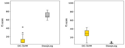
Figure 4: Sensitivity of detection accuracy for semi-supervised traditional and deep learning techniques on HDFS (left) and Hadoop (right).

As depicted in Figure 4, DeepLog is less sensitive to hyperparameter tuning in terms of detection accuracy than OC-SVM on both datasets. On HDFS, its detection accuracy ranges from $59.08$ to $83.23$ (avg $\approx 70.85$, StdDev $\approx 6.58$), whereas the detection accuracy of OC-SVM ranges from $5.70$ to $42.71$ (avg $\approx 13.06$, StdDev $\approx 11.25$). Moreover, on Hadoop, the detection accuracy of DeepLog ranges from $5.96$ to $10.39$ (avg $\approx 6.62$, StdDev $\approx 0.86$), whereas the detection accuracy computed for OC-SVM ranges from $7.14$ to $43.08$ (avg $\approx 28.27$, StdDev $\approx 10.65$).

Sensitivity of Training Time

As depicted in Figure 5, DeepLog is less sensitive to hyperparameter tuning than OC-SVM on HDFS: its model training time ranges from $34.73\text{\,}\mathrm{s}$ to $418.23\text{\,}\mathrm{s}$ (avg $\approx$146.78\text{\,}\mathrm{s}$$, stdDev $\approx$105.43\text{\,}\mathrm{s}$$). OC-SVM takes from $19\,339.39\text{\,}\mathrm{s}$ to $65\,619.39\text{\,}\mathrm{s}$ (avg $\approx$49\,429.95\text{\,}\mathrm{s}$$, stdDev $\approx$13\,036.55\text{\,}\mathrm{s}$$) to train the corresponding model. On Hadoop, OC-SVM outperforms Deeplog, showing a model training time that ranges from $0.01\text{\,}\mathrm{s}$ to $0.05\text{\,}\mathrm{s}$ (avg $\approx$0.04\text{\,}\mathrm{s}$$, stdDev $\approx$0.01\text{\,}\mathrm{s}$$), whereas DeepLog takes from $18.87\text{\,}\mathrm{s}$ to $918.07\text{\,}\mathrm{s}$ (avg $\approx$280.0\text{\,}\mathrm{s}$$, stdDev $\approx$244.68\text{\,}\mathrm{s}$$) for its model training. The reason for which DeepLog takes more time than OC-SVM on Hadoop, although both techniques are trained with the same data set (see Section III), is due to the size of the time window used for DeepLog (see footnote 4). It led to a total of 106104 sequences of log event occurrences, rather than only 567 sequences used for OC-SVM.

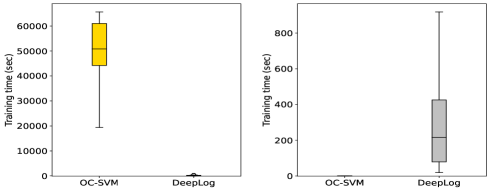
Figure 5: Sensitivity of training time for semi-supervised traditional and deep learning techniques on HDFS (left) and Hadoop (right).

The answer to RQ2, shows that semi-supervised traditional and deep ML techniques do not fare well in terms of detection accuracy. Moreover, the overall performance of the different ML techniques w.r.t. the four evaluation criteria considered in this study, varies across datasets: OC-SVM shows a better detection accuracy, time performance (in terms of model re-training and prediction) and lower sensitivity to hyperparameter tuning, in terms of training time, than DeepLog on Hadoop. DeepLog, however, is more accurate, faster (in terms of model re-training and prediction), and less sensitive to hyperparameter tuning in terms of time performance (training time) than OC-SVM on HDFS, and less sensitive to hyperparameter tuning, in terms of detection accuracy, on both datasets.

VII Discussion

The answer to RQ1 and RQ2 suggests that more attention should be given to traditional supervised ML techniques when it comes to the detection of execution path log anomalies before considering more complex deep ML techniques. The answer to RQ1 shows that RF has a high detection accuracy on both datasets, HDFS and Hadoop. Its computational time is also significantly lower when compared to other supervised traditional and deep learning techniques. Further, RF is not sensitive to hyperparameter settings, on both datasets. RF is therefore our recommendation, at this point, to build prediction models of execution path log anomalies in practice.

Threats to validity. In the following, we discuss three types of threats to validity that can affect the findings of our study.
Internal threats. We relied on publicly available implementations of DeepLog [31] and LogRobust [32]. These third-party implementations might be faulty and could introduce a bias in the results. Further, due to the high computational cost of our experiments, we limited the hyperparameter tuning for each ML technique. More hyperparameter settings would have probably led to better detection accuracy and time performance, though we do not expect drastic differences. Although HDFS was manually inspected and carefully labeled by domain experts, noise in the data is still possible, leading to lower detection accuracy.
External threats. We conducted our experiments on two public benchmark datasets that are widely used in existing studies. Further, only considering two semi-supervised techniques may also affect the generalization of our findings. Therefore, using two datasets and two techniques may not be enough to generalize our findings.

VIII Conclusion and Future Work

In this empirical study, we assessed the detection accuracy and the time performance, in terms of model training and log anomaly prediction, of different semi-supervised and supervised, traditional and deep ML techniques. We further studied the sensitivity of detection accuracy and model training time, for each of these techniques, to hyperparameter tuning across datasets.

The study shows that supervised traditional and deep ML techniques fare similarly in terms of detection accuracy and prediction time. Further, supervised traditional ML techniques far outperform supervised deep learning ones in terms of re-training time. Among the former, Random Forest shows the least sensitivity to hyperparameter tuning w.r.t. its detection accuracy and time performance.

Though they offer practical advantages, semi-supervised techniques yield significantly worse detection accuracy than supervised ML techniques. Time performance and sensitivity to hyperparameter tuning of semi-supervised traditional and deep ML techniques, in terms of detection accuracy and time performance, vary across datasets.

Though they need to be confirmed with further studies, the results above are of practical importance because they suggest—when accounting for accuracy, training and prediction time, and sensitivity to hyperparameter tuning—that supervised, traditional techniques are a better option for log anomaly detection, with a preference for Random Forest. Given the emphasis on the use of deep learning in the research literature, this may come as a surprise.

Detecting log anomalies is not sufficient for system engineers as it does not provide them with enough details about the cause(s) of anomalies. This warrants the design of solutions to facilitate the diagnosis of anomalies.

References

- [1] M. Du, F. Li, G. Zheng, and V. Srikumar, “Deeplog: Anomaly detection and diagnosis from system logs through deep learning,” in Proceedings of the 2017 ACM SIGSAC conference on computer and communications security, 2017, pp. 1285–1298.
- [2] B. Zhu, J. Li, R. Gu, and L. Wang, “An approach to cloud platform log anomaly detection based on natural language processing and lstm,” in 2020 3rd International Conference on Algorithms, Computing and Artificial Intelligence, 2020, pp. 1–7.
- [3] Y. Xie, L. Ji, and X. Cheng, “An attention-based gru network for anomaly detection from system logs,” IEICE TRANSACTIONS on Information and Systems, vol. 103, no. 8, pp. 1916–1919, 2020.
- [4] S. Huang, Y. Liu, C. Fung, R. He, Y. Zhao, H. Yang, and Z. Luan, “Hitanomaly: Hierarchical transformers for anomaly detection in system log,” IEEE Transactions on Network and Service Management, vol. 17, no. 4, pp. 2064–2076, 2020.
- [5] X. Liu, W. Liu, X. Di, J. Li, B. Cai, W. Ren, and H. Yang, “Lognads: Network anomaly detection scheme based on log semantics representation,” Future Generation Computer Systems, vol. 124, pp. 390–405, 2021.
- [6] W. Meng, Y. Liu, Y. Zhu, S. Zhang, D. Pei, Y. Liu, Y. Chen, R. Zhang, S. Tao, P. Sun et al., “Loganomaly: Unsupervised detection of sequential and quantitative anomalies in unstructured logs.” in IJCAI, vol. 19, no. 7, 2019, pp. 4739–4745.
- [7] L. Yang, J. Chen, Z. Wang, W. Wang, J. Jiang, X. Dong, and W. Zhang, “Semi-supervised log-based anomaly detection via probabilistic label estimation,” in 2021 IEEE/ACM 43rd International Conference on Software Engineering (ICSE). IEEE, 2021, pp. 1448–1460.
- [8] X. Zhang, Y. Xu, Q. Lin, B. Qiao, H. Zhang, Y. Dang, C. Xie, X. Yang, Q. Cheng, Z. Li et al., “Robust log-based anomaly detection on unstable log data,” in Proceedings of the 2019 27th ACM Joint Meeting on European Software Engineering Conference and Symposium on the Foundations of Software Engineering, 2019, pp. 807–817.
- [9] S. Lu, X. Wei, Y. Li, and L. Wang, “Detecting anomaly in big data system logs using convolutional neural network,” in 2018 IEEE 16th Intl Conf on Dependable, Autonomic and Secure Computing, 16th Intl Conf on Pervasive Intelligence and Computing, 4th Intl Conf on Big Data Intelligence and Computing and Cyber Science and Technology Congress (DASC/PiCom/DataCom/CyberSciTech). IEEE, 2018, pp. 151–158.
- [10] Z. Wang, J. Tian, H. Fang, L. Chen, and J. Qin, “Lightlog: A lightweight temporal convolutional network for log anomaly detection on the edge,” Computer Networks, vol. 203, p. 108616, 2022.
- [11] V.-H. Le and H. Zhang, “Log-based anomaly detection without log parsing,” in 2021 36th IEEE/ACM International Conference on Automated Software Engineering (ASE). IEEE, 2021, pp. 492–504.
- [12] H. Guo, S. Yuan, and X. Wu, “Logbert: Log anomaly detection via bert,” in 2021 international joint conference on neural networks (IJCNN). IEEE, 2021, pp. 1–8.
- [13] J. Qi, Z. Luan, S. Huang, C. Fung, H. Yang, H. Li, D. Zhu, and D. Qian, “Logencoder: Log-based contrastive representation learning for anomaly detection,” IEEE Transactions on Network and Service Management, 2023.
- [14] J. Chen, W. Chong, S. Yu, Z. Xu, C. Tan, and N. Chen, “Tcn-based lightweight log anomaly detection in cloud-edge collaborative environment,” in 2022 Tenth International Conference on Advanced Cloud and Big Data (CBD). IEEE, 2022, pp. 13–18.
- [15] P. He, J. Zhu, Z. Zheng, and M. R. Lyu, “Drain: An online log parsing approach with fixed depth tree,” in 2017 IEEE international conference on web services (ICWS). IEEE, 2017, pp. 33–40.
- [16] V.-H. Le and H. Zhang, “Log-based anomaly detection with deep learning: How far are we?” in Proceedings of the 44th International Conference on Software Engineering, ser. ICSE ’22. New York, NY, USA: Association for Computing Machinery, 2022, pp. 1356–1367. [Online]. Available: https://doi.org/10.1145/3510003.3510155
- [17] M. Zhang, J. Chen, J. Liu, J. Wang, R. Shi, and H. Sheng, “Logst: Log semi-supervised anomaly detection based on sentence-bert,” in 2022 7th International Conference on Signal and Image Processing (ICSIP). IEEE, 2022, pp. 356–361.
- [18] L. Wang, Support vector machines: theory and applications. Springer Science & Business Media, 2005, vol. 177.
- [19] L. Breiman, “Random forests,” Machine learning, vol. 45, pp. 5–32, 2001.
- [20] S. Hochreiter and J. Schmidhuber, “Long short-term memory,” Neural computation, vol. 9, no. 8, pp. 1735–1780, 1997.
- [21] B. Schölkopf, J. C. Platt, J. Shawe-Taylor, A. J. Smola, and R. C. Williamson, “Estimating the support of a high-dimensional distribution,” Neural computation, vol. 13, no. 7, pp. 1443–1471, 2001.
- [22] M. Landauer, S. Onder, F. Skopik, and M. Wurzenberger, “Deep learning for anomaly detection in log data: A survey,” arXiv preprint arXiv:2207.03820, 2022.
- [23] A. Joulin, E. Grave, P. Bojanowski, M. Douze, H. Jégou, and T. Mikolov, “Fasttext. zip: Compressing text classification models,” arXiv preprint arXiv:1612.03651, 2016.
- [24] G. Salton and C. Buckley, “Term-weighting approaches in automatic text retrieval,” Information processing & management, vol. 24, no. 5, pp. 513–523, 1988.
- [25] S. He, J. Zhu, P. He, and M. R. Lyu, “Loghub: a large collection of system log datasets towards automated log analytics,” arXiv preprint arXiv:2008.06448, 2020.
- [26] W. Xu, L. Huang, A. Fox, D. Patterson, and M. I. Jordan, “Detecting large-scale system problems by mining console logs,” in Proceedings of the ACM SIGOPS 22nd symposium on Operating systems principles, 2009, pp. 117–132.
- [27] A. Oliner and J. Stearley, “What supercomputers say: A study of five system logs,” in 37th annual IEEE/IFIP international conference on dependable systems and networks (DSN’07). IEEE, 2007, pp. 575–584.
- [28] Q. Lin, H. Zhang, J.-G. Lou, Y. Zhang, and X. Chen, “Log clustering based problem identification for online service systems,” in Proceedings of the 38th International Conference on Software Engineering Companion, 2016, pp. 102–111.
- [29] J. N. Van Rijn and F. Hutter, “Hyperparameter importance across datasets,” in Proceedings of the 24th ACM SIGKDD International Conference on Knowledge Discovery & Data Mining, 2018, pp. 2367–2376.
- [30] J. Bergstra and Y. Bengio, “Random search for hyper-parameter optimization.” Journal of machine learning research, vol. 13, no. 2, 2012.
- [31] wuyifan18, “Pytorch implementation of deeplog.” https://github.com/wuyifan18/DeepLog, 2020.
- [32] V.-H. Le and H. Zhang, “Log-based anomaly detection with deep learning: How far are we?” https://github.com/LogIntelligence/LogADEmpirical, 2022.
Acknowledgments
This work was supported by a research grant from Auxon Corporation, Mitacs Canada, as well as the Canada Research Chair and Discovery Grant programs of the Natural Sciences and Engineering Research Council of Canada (NSERC). The experiments conducted in this work were enabled in part by the computation support provided by Compute Canada 101010https://www.computecanada.ca.