Deep Learning Meets Adaptive Filtering:
A Stein’s Unbiased Risk Estimator Approach

Abstract

This paper revisits two prominent adaptive filtering algorithms, namely recursive least squares (RLS) and equivariant adaptive source separation (EASI), through the lens of algorithm unrolling. Building upon the unrolling methodology, we introduce novel task-based deep learning frameworks, denoted as Deep RLS and Deep EASI. These architectures transform the iterations of the original algorithms into layers of a deep neural network, enabling efficient source signal estimation by leveraging a training process. To further enhance performance, we propose training these deep unrolled networks utilizing a surrogate loss function grounded on Stein’s unbiased risk estimator (SURE). Our empirical evaluations demonstrate that the Deep RLS and Deep EASI networks outperform their underlying algorithms. Moreover, the efficacy of SURE-based training in comparison to conventional mean squared error loss is highlighted by numerical experiments. The unleashed potential of SURE-based training in this paper sets a benchmark for future employment of SURE either for training purposes or as an evaluation metric for generalization performance of neural networks.

I Introduction

Deep unfolding, or unrolling [1], enables constructing interpretable deep neural networks (DNN) that require less training data and considerably less computational resources than generic DNNs. Specifically, in deep unfolding, each layer of the DNN is designed to resemble one iteration of the original algorithm of interest. Passing the signals through such a deep network is in essence similar to executing the iterative algorithm a finite number of times, determined by the number of layers. The model parameters will be reflected in weights of the constructed DNN. The data-driven nature of the emerging deep network thus enables improvements over the original algorithm. Note that the constructed network may be trained using back-propagation, resulting in model parameters that are learned from the real-world training datasets. In this way, the trained network can be naturally interpreted as a parameter optimized algorithm, effectively overcoming the lack of interpretability in most conventional neural networks [2]. In comparison with a generic DNN, the unfolded network has many fewer parameters and therefore requires a more modest size of training data and computational resources.

The deep unrolling technique has been effectively applied to various signal processing problems, yielding significant improvements in the convergence rates of state-of-the-art iterative algorithms; see [2, 1] for a detailed explanation of deep unrolling, as well as [3, 4, 5] for examples of deploying deep unrolling in different application areas.

Our goal in this paper is to develop a set of algorithms able to learn the nonlinearity and step sizes of two classical adaptive filtering algorithms, namely, recursive least squares (RLS) and equivariant adaptive source separation (EASI). We leverage Stein’s unbiased risk estimator (SURE) in training, which serves as a surrogate for mean squared error (MSE), even when the ground truth is unknown [6]. Studies such as [7, 8] have reported improved image denoising results when networks were trained with SURE loss, outperforming traditional MSE loss training. Similarly, SURE has been effectively used to train deep convolutional neural networks without requiring denoised ground truth, as highlighted in [7, 9]. The SURE based training and the recurrent training procedure of our proposed methodology makes it a great candidate for unsupervised real-time signal processing.

The rest of the paper is organized in the following manner. In section II, we introduce the problem formulation for adaptive filtering-based signal estimation. In Section III, we propose the two deep unrolling frameworks Deep EASI and Deep RLS for adaptive filtering, alongside the SURE-based surrogate loss function employed for their training. Section IV details the numerical experiments used to evaluate our proposed methods, and Section V presents our concluding remarks.

Notation: Throughout this paper, we use bold lowercase and bold uppercase letters for vectors and matrices, respectively. $\mathbb{R}$ represents the set of real numbers. $(\cdot)^{\top}$ denotes the vector/matrix transpose. The identity matrix of is denoted by $\mathbf{I}$ and the trace of a matrix is denoted by $\operatorname{Tr}(.)$.

II Problem formulation

We begin by the long-standing linear inference problem formulation in which $m$ statistically independent signals are linearly mixed to yield $l$ possibly noisy combinations,

$$\mathbf{x}(t)=\mathbf{A}\mathbf{s}(t)+\mathbf{n}(t).$$ (1)

Let $\mathbf{x}(t)=[\mathbf{x}_{1}(t),\ldots,\mathbf{x}_{l}(t)]^{\top}$ denote the $l-$dimensional data vector made up of the mixture at time $t$ that is exposed to an additive measurement noise $\mathbf{n}(t)$. Given no knowledge of the mixing matrix $\mathbf{A}\in\mathds{R}^{m\times l}$, the goal is to recover the original source signal vector $\mathbf{s}(t)=[\mathbf{s}_{1}(t),\ldots,\mathbf{s}_{m}(t)]^{\top}$ from the mixture. This problem is referred to as blind source separation (BSS) in the literature. A seminal work in this context is [10] which suggests tuning and updating a separating matrix $\mathbf{W}\in\mathds{R}^{l\times m}$ until the output

$$\mathbf{y}(t)=\mathbf{W}^{\top}\mathbf{x}(t),$$ (2)

where $\mathbf{y}(t)=[\mathbf{y}_{1}(t),\ldots,\mathbf{y}_{m}(t)]^{\top}$, is as close as possible to the source signal vector of interest $\mathbf{s}(t)$.

II-A Nonlinear Recursive Least Squares for Blind Source Separation

Assuming there exists a larger number of sensors than the source signals, i.e. $l\geq m$, we can draw an analogy between the BSS problem and the task of principal component analysis (PCA). In a sense, we are aiming to represent the random vector $\mathbf{x}(t)$ in a lower dimensional orthonormal subspace, represented by the columns of $\mathbf{W}$, as the orthonormal basis vectors. By this analogy, both BSS and PCA problems can be reduced to minimizing the objective function

$$\mathcal{L}(\mathbf{W})=\mathbb{E}\left\{\|\mathbf{x}(t)-\mathbf{W}(\mathbf{W}^{\top}\mathbf{x}(t))\|_{2}^{2}\right\}.$$ (3)

Assuming that $\mathbf{x}(t)$ is a zero-mean vector, it can be shown that the solution to the above optimization problem is a matrix $\mathbf{W}$ whose columns are the $m$ dominant eigenvectors of the data covariance matrix $\mathbf{C_{x}(t)}=\mathbb{E}\left\{\mathbf{x}(t)\mathbf{x}(t)^{\top}\right\}$ [11]. Therefore, the principal components which are the recovered source signals are mutually uncorrelated. As discussed in [10], having uncorrelated data is not a sufficient condition to achieve separation. In other words, the solutions to PCA and BSS do not coincide unless we address the higher order statistics of the output signal $\mathbf{y}(t)$. By introducing nonlinearity into (3), we will implicitly target higher order statistics of the signal [11]. This nonlinear PCA, which is an extension of the conventional PCA, is made possible by considering the signal recovery objective:

$$\mathcal{L}(\mathbf{W})=\mathbb{E}\left\{\|\mathbf{x}(t)-\mathbf{W}\mathbf{g}(\mathbf{W}^{\top}\mathbf{x}(t))\}\|_{2}^{2}\right\},$$ (4)

where $\mathbf{g}(\cdot)$ denotes an odd non-linear function applied element-wise on the vector argument. The proof of the connection between (4) and higher order statistics of the source signals $\mathbf{s}(t)$ is discussed in [12]. While PCA is a fairly standardized technique, nonlinear or robust PCA formulations based on (4) tend to be multi-modal with several local optima—so they can be run from various initial points and possibly lead to different “solutions” [13]. In [14], a recursive least squares algorithm for subspace estimation is proposed, which is further extended to the nonlinear PCA in [15] for solving the BSS problem. The algorithm in [15] is useful as a baseline for developing our deep unfolded framework for nonlinear PCA.

We consider a real-time and adaptive scenario in which, upon arrival of new data $\mathbf{x}(t)$, the subspace of signal at time instant $t$ is recursively updated from the subspace at time $t-1$ and the new sample $\mathbf{x}(t)$ [14]. The separating matrix $\mathbf{W}$ introduced in (4) is therefore replaced by $\mathbf{W}(t)$ and updated at each time instant $t$. The adaptive algorithm chosen for this task is the well-known recursive least squares (RLS) [16]. In the linear case, by replacing the expectation in (3) with a weighted sum, we can attenuate the impact of the older samples, which is reasonable for a time-varying environment. In this way, one can make sure the distant past will be forgotten and the resulting algorithm for minimizing (3) can effectively track the statistical variations of the observed data. By replacing $\mathbf{y}(t)=\mathbf{W}(t)^{\top}\mathbf{x}(t)$ and using an exponential weighting (governed by a forgetting factor), the loss function in (3) boils down to:

$$\mathcal{L}(\mathbf{W})=\sum_{i=1}^{t}\beta^{t-i}\|\mathbf{x}(i)-\mathbf{W}(t)\mathbf{y}(i)\|^{2},$$ (5)

with the forgetting factor $\beta$ satisfying $0\ll\beta\leq 1$. Note that $\beta=1$ yields the ordinary method of least squares in which all samples are weighed equally while choosing relatively small $\beta$ makes our estimation rather instantaneous, thus neglecting the past. Therefore, $\beta$ is usually chosen to be less than one, but also rather close to one for smooth tracking and filtering.

We can write the gradient of the loss function in (5) in its compact form as

$$\nabla_{\mathbf{W}(t)}\mathcal{L}(\mathbf{W})=-2\mathbf{C_{xy}}(t)+2\mathbf{C_{y}}(t)\mathbf{W}(t),$$ (6)

where $\mathbf{C_{y}}(t)$ and $\mathbf{C_{xy}}(t)$ are the auto-correlation matrix of $\mathbf{y}(t)$,

$$\mathbf{C_{y}}(t)=\sum_{i=1}^{t}\beta^{t-i}\mathbf{y}(i)\mathbf{y}(i)^{\top}=\beta\mathbf{C_{y}}(t-1)+\mathbf{y}(t)\mathbf{y}(t)^{\top},$$ (7)

and the cross-correlation matrix of $\mathbf{x}(t)$ and $\mathbf{y}(t)$,

$$\mathbf{C_{xy}}(t)=\sum_{i=1}^{t}\beta^{t-i}\mathbf{x}(i)\mathbf{y}(i)^{\top}=\beta\mathbf{C_{xy}}(t-1)+\mathbf{x}(t)\mathbf{y}(t)^{\top},$$ (8)

at the time instance $t$, respectively. Setting the gradient (6) to zero will result in the close-form separating matrix

$$\mathbf{W}(t)=\mathbf{C_{y}}^{-1}(t)\mathbf{C_{xy}}(t).$$ (9)

A recursive computation of $\mathbf{W}(t)$ can be achieved using the RLS algorithm [17]. In RLS, the matrix inversion lemma enables a recursive computation of $\mathbf{G}(t)=\mathbf{C_{y}}^{-1}(t)$; see the derivations in Appendix. At each iteration of the RLS algorithm, $\mathbf{G}(t)$ is computed recursively as

$$\mathbf{G}(t)=\beta^{-1}\mathbf{G}(t-1)-\frac{\beta^{-2}\mathbf{G}(t-1)\mathbf{y}(t)\mathbf{y}(t)^{\top}\mathbf{G}(t-1)}{1+\beta^{-1}\mathbf{y}(t)^{\top}\mathbf{G}(t-1)\mathbf{y}(t)}.$$ (10)

Consequently, the RLS algorithm provides the estimate $\mathbf{y}(t)$ of the source signals. The steps of the RLS algorithm are summarized in Algorithm 1. It appears that extending the application of RLS to the nonlinear PCA loss function in (4) is rather straightforward. To accomplish this task, solely step 3 of Algorithm 1 should be modified to $\mathbf{y}(t)=g(\mathbf{W}^{\top}(t-1)\mathbf{x}(t))$ in order to meet the nonlinear PCA criterion [14].

Algorithm 1 RLS Algorithm for Performing PCA

1:Initialize $\mathbf{W}(0)$ and $\mathbf{G}(0)$

2:for $t=0,1,\ldots,T$ do

3:      $\mathbf{y}(t)=\mathbf{W}^{\top}(t-1)\mathbf{x}(t)$

4:      $\mathbf{h}(t)=\mathbf{G}(t-1)\mathbf{y}(t)$

5:      $\mathbf{f}(t)=\frac{\mathbf{h}(t)}{\beta+\mathbf{y}(t)^{\top}\mathbf{h}(t)}$

6:      $\mathbf{G}(t)=\beta^{-1}[\mathbf{G}(t-1)-\mathbf{f}(t)\mathbf{h}(t)^{\top}]$

7:      $\mathbf{e}(t)=\mathbf{x}(t)-\mathbf{W}(t-1)\mathbf{y}(t)$

8:      $\mathbf{W}(t)=\mathbf{W}(t-1)+\mathbf{e}(t)\mathbf{f}(t)^{\top}$

In order for the RLS algorithm to optimize the nonlinear PCA loss function and converge to a separating matrix the choice of nonlinearity g(.) matters. We refer to the analytical study presented in [13] in which some conditions beyond the oddity and differentiability of the function g(.) must be satisfied. For instance, $g(s)=s^{3}$ leads to an asymptotically stable separation only if the source signals are positively kurtotic or super-Gaussian. Whereas if we choose a sigmoidal nonlinearity $g(s)=tanh(\beta s)$ with $\beta>0$, then a sub-Gaussian density is required for the source signals to be separated using RLS algorithm.

In section III-A, we unroll the iterations of the modified Algorithm 1, for nonlinear PCA onto the layers of a deep neural network where each layer resembles one iteration of the RLS algorithm.

II-B Equivariant Adaptive Source Separation (EASI)

In [10], the EASI algorithm is developed by recurrent updates of the separating matrix as

$$\mathbf{W}(t+1)=\mathbf{W}(t)-\lambda_{t}\mathbf{H}(\mathbf{y}(t))\mathbf{W}(t).$$ (11)

Where $\lambda_{t}$ is a sequence of positive step sizes and $\mathbf{H}(.)$ is a matrix valued function used to update the separating matrix. In [10] this function is calculated as the relative gradient with respect to the objective function for blind source separation. The cross-cumulants of the source signals in $\mathbf{y}(t)$ is proposed as the objective function to be minimized as a measure of independence. $\mathbf{H}(.)$ is derived in [10] as

$$\mathbf{H}(\mathbf{y}(t))=\mathbf{y}(t)\mathbf{y}(t)^{\top}-\mathbf{I}+g(\mathbf{y}(t))\mathbf{y}(t)^{\top}-\mathbf{y}(t)g(\mathbf{y}(t))^{\top}$$ (12)

where l arbitrary nonlinear functions, $g_{1}(.),g_{2}(.),\ldots,g_{l}(.)$ are used to define

$$g(\mathbf{y}(t))=[g_{1}(\mathbf{y}_{1}(t)),\ldots,g_{l}(\mathbf{y}_{l}(t))]^{\top}.$$ (13)

The choice of this nonlinear function is crucial to the performance of the algorithm and is dependent on the distribution of sources. For instance, for sources with identical distibutions $g_{i}(.)=g(.)$ will be sufficient to perform seperation. In [10], it is illustrated that a cubic nonlinearity $g(s)=s^{3}$ leads to stability of separation in EASI algorithm only under the constraint that sum of kurtosis of any two source signals $s_{i}$ and $s_{j}$, $1\leq i,j\leq m$ are negative. $g(s)=tanh(s)$ is reported in [15] to work satisfactorily for two sub-Gaussian sources using $\lambda_{t}>0$. The nonlinear PCA algorithm require that the original source signals have a kurtosis with the same sign. Although this condition is somehow relaxed in the EASI algorithm so that the sum of kurtosises for any pair of two sources must be negative, still some knowledge on the probability distribution of source signals is required to choose the nonlinearity. In the following sections, we propose to learn the nonlinearity in  (13) along with the step size in (11) using deep unfolding networks.

III The Proposed Framework

The estimation performance of the algorithms discussed above depends on a number of factors such as condition of mixing matrix $\mathbf{A}$, source signals, the step size parameter(s) and nonlinearity $g(.)$. We propose to overparameterize the algorithms so that we can determine the optimal stepsize and proper nonlinearities as apposed to using fixed parameters. In this section, we present the proposed deep architectures Deep RLS in III-A and Deep EASI in III-B. The training procedure for these two architectures and the SURE based loss function will be introduced in III-C and III-D, respectively.

III-A Deep RLS

As shown in [15], when applied to a linear mixture of source signals (i.e., the BSS problem), the RLS algorithm usually approximates the true source signals well and successfully separates them. However, the number of iterations needed to converge may vary greatly depending on the initial values $\mathbf{W}(0),\mathbf{G}(0)$ and the forgetting parameter $\beta$. We introduce Deep RLS, our deep unrolling-based framework which is designed based on the modified iterations of the algorithm 1. More precisely, the dynamics of the $k$-th layer of Deep RLS are given as:

$$\mathbf{y}(k) =\mathbf{g}_{{}_{\nu_{k}}}(\mathbf{W}^{\top}(k-1)\mathbf{x}(k)),$$ (14)

$$\mathbf{h}(k) =\mathbf{G}(k-1)\mathbf{y}(k),$$ (15)

$$\mathbf{f}(k) =\frac{\mathbf{h}(k)}{\mathbf{\omega}_{k}+\mathbf{y}(k)^{\top}\mathbf{h}(k)},$$ (16)

$$\mathbf{G}(k) =\omega_{k}^{-1}[\mathbf{G}(k-1)-\mathbf{f}(k)\mathbf{h}(k)^{\top}],$$ (17)

$$\mathbf{e}(k) =\mathbf{x}(k)-\mathbf{W}(k-1)\mathbf{y}(k),$$ (18)

$$\mathbf{W}(k) =\mathbf{W}(k-1)+\mathbf{e}(k)\mathbf{f}(k)^{\top},$$ (19)

where $\mathbf{x}(k)$ is the data vector at time instance $k$. The nonlinearity $\mathbf{g}(\cdot)$ in the original RLS algorithm, which was chosen accroding to the distribution of the source signals, is overparameterized to $\mathbf{g}_{{}_{\nu_{k}}}(\cdot)$. Considering that neural networks with at least one hidden layer are universal approximators and they can be trained to approximate any mapping, we use a set of fully connected layers as $\mathbf{g}_{{}_{\nu_{k}}}(\cdot)$. Weights and biases of these layers are represented by the learnable parameter $\nu_{k}$ and $\omega_{k}\in\mathds{R}$ represents the trainable forgetting parameter.

Given $T$ samples of the data vector $\mathbf{x}(t)$, our goal is to optimize the parameters $\boldsymbol{\Gamma}$ of the network, where

$$\boldsymbol{\Gamma}=\{\nu_{k},\mathbf{\omega}_{k}\}_{k=1}^{T}.$$ (20)

The output of the $k$-th layer, i.e. $\mathbf{y}(k)$, in (14) is an approximation of the source signals at the time instance $k$.

III-B Deep EASI

We consider the EASI iterations defined in (11) as our baseline to reconstruct the unfolded network. We over parameterize the iterations by introducing a learnable step-size $\lambda_{t}$ and $\mathbf{H}_{\phi_{t}}$ for each layer $t$ as

$$\mathbf{W}(t+1)=\mathbf{W}(t)-\lambda_{t}\mathbf{H}_{\phi_{t}}(\mathbf{y}(t))\mathbf{W}(t)$$ (21)

and

$$\mathbf{H}_{\phi_{t}}(\mathbf{y}(t))=\mathbf{y}(t)\mathbf{y}(t)^{\top}-\mathbf{I}+g_{\phi_{t}}(\mathbf{y}(t))\mathbf{y}(t)^{\top}-\mathbf{y}(t)g_{\phi_{t}}(\mathbf{y}(t))^{\top},$$ (22)

where $g_{\phi_{t}}(.)$ is realized using a few layers of fully connected layers, with weights $\phi_{t}$, deployed to approximate the best nonlinearity for separation. The trainable parameters of the network will be

$$\boldsymbol{\theta}=\{\phi_{t},\lambda_{t}\}_{t=1}^{T}$$ (23)

The output of the $t$-th layer, i.e. $\mathbf{y}(t)$ is

$$\mathbf{y}(t)=\mathbf{W}(t)^{\top}\mathbf{x}(t),$$ (24)

III-C Training Procedure

An earlier version of this work proposed in [19] and was successful in recovering the source signals. However, it could only use a few number of inputs $\mathbf{x}(t)$ because deeper networks with huge number of parameters were not feasible to be trained. Parameter sharing is a technique in deep learning which regularizes the network to avoid this problem. Parameter sharing makes it possible to extend and apply the model to signals of different lengths and generalize across them. In Deep RLS architecture proposed in [19], we designed a multi-layer feedforward neural network in which we had separate learnable parameters for each time index and we could not generalize to sequence lengths not seen during training. Recurrent Neural Networks (RNN) are introduced to overcome this limitation. Inspired by the architecture of these neural networks and back-propagation through time (BPTT) as their training process, we propose the following loss function for training the proposed unrolled algortihms. An RNN maps an input sequence to an output sequence of the same length. The total loss for a given sequence of $\mathbf{x}(t)$ values paired with a sequence of $\mathbf{y}(t)$ values is the sum of the losses over all the time steps. For example, if $L(t)$ is the mean squared error (MSE) of reconstructing $\mathbf{s}(t)$ given $\mathbf{y}(t)$ then

$$\mathcal{L}(\mathbf{s},\mathbf{y})=\sum_{t=1}^{T}L{(t)}=\sum_{t=1}^{T}\|\mathbf{s}(t)-\mathbf{y}(t)\|^{2}_{2},$$ (25)

where $\mathbf{y}=[\mathbf{y}(1),\ldots,\mathbf{y}(T)]^{\top}$ and $\mathbf{s}=[\mathbf{s}(1),\ldots,\mathbf{s}(T)]^{\top}$. In order to apply BPTT, the gradient of the loss function $L(t)$ with respect to the trainable parameters is required. This is challenging to do by hand, but made easy by the auto-differentiation capabilities is PyTorch [20], which is used throughout our experiments in section IV.

While training Deep RLS, one needs to consider the constraint that the forgetting parameter must satisfy $0<\beta\leq 1$. Hence, in order to impose such a constraint, one can regularize the loss function ensuring that the network chooses proper weights $\{\omega_{k}\}_{k=1}^{T}$ corresponding to a feasible forgetting parameter at each layer. Accordingly, we define the loss function used for training the proposed architecture as

$$\begin{split}\mathcal{L}(\mathbf{s},\mathbf{y},\Gamma)&=\sum_{t=1}^{T}\|\mathbf{s}(t)-\mathbf{y}(t)\|^{2}_{2}+\\ &\underbrace{\lambda\sum_{t=1}^{T}\mathrm{ReLU}(-\mathbf{\omega}_{t})+\lambda\sum_{t=1}^{T}\mathrm{ReLU}(\mathbf{\omega}_{t}-1)}_{\text{regularization term for the forgetting parameter}},\end{split}$$ (26)

where $\mathrm{ReLU}(\cdot)$ is the well-known Rectifier Linear Unit function extensively used in the deep learning literature. For training the Deep RLS (or Deep EASI) network we employed the training process in Algorithm 2.

Algorithm 2 Training Procedure for Deep RLS(or Deep EASI).

1:Initialize $\mathbf{W}(0)$ and $\mathbf{\mathbf{G}}(0)$

2:for $\textrm{epoch}=1,\ldots,N$ do

3:     for $t=1,\ldots,T$ do

4:          Feed $\mathbf{x}(t)$ to the network

5:          Apply the recursion in (14)-(19) (or (21))

6:          Compute the loss function in (26) (or (25))

7:          Use BPTT to update $\boldsymbol{\Gamma}$ (or $\boldsymbol{\theta}$)      

III-D Stein’s Unbiased Risk Estimator (SURE)

In 1981 Charles Stein in [21] showed that for $\mathbf{x}=\boldsymbol{\mu}+\boldsymbol{n}$ and $\mathbf{n}\sim\mathcal{N}(\boldsymbol{0},\sigma^{2}\mathbf{I})$, the SURE statistic defined as

$$\text{SURE}(\hat{\boldsymbol{\mu}},\mathbf{x})=-l\sigma^{2}+\|\hat{\boldsymbol{\mu}}(\mathbf{x})-\mathbf{x}\|^{2}_{2}+2\sigma^{2}\nabla\hat{\boldsymbol{\mu}}(\mathbf{x})$$ (27)

is an unbiased estimate of the $l_{2}$ risk of the estimator $\hat{\boldsymbol{\mu}}$ in the sense that $\mathds{E}\left\{{\text{SURE}}\right\}=\mathds{E}\left\{{\|\hat{\boldsymbol{\mu}}(\mathbf{x})-\boldsymbol{\mu}\|^{2}}\right\}$. The bottleneck in evaluation of SURE is evaluation of the divergence $\nabla\hat{\boldsymbol{\mu}}(\mathbf{x})=\sum\frac{\partial\hat{\boldsymbol{\mu}_{i}}(\mathbf{x})}{\partial x_{i}}$. A generalization of this technique known as generalized SURE was proposed in [22] to estimate the MSE associated with estimates of $\mathbf{s}$ from linear measurements $\mathbf{x}=\mathbf{A}\mathbf{s}+\mathbf{n}$, where $\mathbf{A}\neq\mathbf{I}$, and $\mathbf{n}$ has known covariance and follows any distribution from the exponential family. For the estimators $f_{\boldsymbol{\theta}}(.)$ parameterized over $\boldsymbol{\theta}$ which receive the noisy observation $\mathbf{x}$ and provide an estimate of sources $\mathbf{s}$, expectation of the generalized SURE is [7]

$$\mathbb{E}\{\|\hat{\mathbf{s}}-\mathbf{s}\|_{2}^{2}\}$$

$$=\mathbb{E}\{\|\mathbf{P}\mathbf{s}-\mathbf{P}f_{\boldsymbol{\theta}}(\mathbf{x})\|_{2}^{2}\}=\mathbb{E}\{\|\mathbf{P}\mathbf{s}\|_{2}^{2}+\|\mathbf{P}f_{\theta}(\mathbf{x})\|_{2}^{2}$$

$$+2\sigma^{2}\nabla(f_{\boldsymbol{\theta}}(\mathbf{x}))-2f_{\boldsymbol{\theta}}(\mathbf{x})^{\top}\mathbf{A}^{\dagger}\mathbf{x}\},$$ (28)

where the orthonormal projection onto the range space of $\mathbf{A}$ is represented by $\mathbf{P}=\mathbf{A}(\mathbf{A}^{\top}\mathbf{A})^{-1}\mathbf{A}^{\top}$ and $\mathbf{A}^{\dagger}$ is the pseudoinverse of $\mathbf{A}$.

The last three terms in (III-D) are dependant on the parameters of the estimator i.e. $\boldsymbol{\theta}$. Considering layer $t$ of Deep EASI as an estimator of the source signal $\mathbf{x}(t)$, we propose to train the network’s parameters $\boldsymbol{\theta}$ by incorporating the SURE loss at time $t$ as

$$L(t)=\|\mathbf{P}f_{\boldsymbol{\theta}}(\mathbf{x}(t))\|^{2}+\\ 2\sigma^{2}\nabla(f_{\boldsymbol{\theta}}(\mathbf{x}(t)))-2f_{\boldsymbol{\theta}}(\mathbf{x}(t))^{\top}\mathbf{A}^{\dagger}\mathbf{x}(t).$$ (29)

In this equation, the Deep EASI network, as an estimator for source signal at time instance $t$, is denoted by $f_{\boldsymbol{\theta}}(\mathbf{x}(t))$. Consequently, the divergence is

$$\nabla(f_{\boldsymbol{\theta}}(\mathbf{x}(t))) =\sum_{i=1}^{l}\frac{\partial f_{\boldsymbol{\theta}}(\mathbf{x}(t))}{\partial\mathbf{x}_{i}}$$

$$=\sum\frac{\partial}{\partial x_{i}}(\mathbf{W}(t)^{\top}\mathbf{x}(t))$$

$$=\operatorname{Tr}(\mathbf{W}(t)).$$ (30)

By Substituting (III-D) in (29), the SURE loss function for training the Deep EASI network is

$$\mathcal{L}(\mathbf{A},\mathbf{x})=\sum_{t=1}^{T}L{(t)}$$ (31)

$$=\sum_{t=1}^{T}\|\mathbf{P}f_{\boldsymbol{\theta}}(\mathbf{x}(t))\|^{2}+2\sigma^{2}\operatorname{Tr}(\mathbf{W}(t))-2f_{\boldsymbol{\theta}}(\mathbf{x}(t))^{\top}\mathbf{A}^{\dagger}\mathbf{x}(t).$$

It is worth mentioning that as discussed in [23], the SURE loss function can not be analytically derived for all estimators but it can be tractably evaluated using the methods introduced in [23]. We leave derivation of this loss for deep RLS for future extension of this study.

While training Deep EASI and Deep RLS, we synthetically produce the observations $x(t)$ for $t=1,\ldots,T$ to use as the training set. Therefore, we have access to the sources $\mathbf{s}(t)$, the mixing matrix $\mathbf{A}$ and the variance of noise $\sigma^{2}$. Therefore evaluation of Evaluating the SURE loss in (29) is possible while training the network. Backpropagation on the SURE Loss function is feasible by means of PyTorch’s auto-differentiation capabilities, which is used throughout much of our experiments below.

The blindness of our method refers to the test in which we only observe the mixtures. In our numerical experiments, we will deploy the SURE loss function in (29) for training the Deep EASI network and illustrate the performance improvement over the initially proposed loss function in (25). Evaluating the SURE loss in (29) does not require the ground truth $\mathbf{s}(t)$ and therefore the learning procedure will be unsupervised.

IV Numerical Study

In this section, we demonstrate the performance of the proposed Deep RLS and Deep EASI algorithms. The proposed framework was implemented using the PyTorch library [20] and the Adam stochastic optimizer [24] with a constant learning rate of $10^{-4}$ for training purposes. The training was performed based on the data generated via the following model. For each time interval $t=0,1,...,T$, elements of the vector $\mathbf{s}(t)$ is generated from a sub-Gaussian distribution. For data generation purposes, we have assumed the source signals to be i.i.d. and uniformly distributed, i.e., $\mathbf{s}(t)\sim\mathcal{U}(0,\boldsymbol{1})$. The mixing matrix $\mathbf{A}$ is assumed to be generated according to $\mathbf{A}\sim\mathcal{N}(\mathbf{0},\mathbf{I})$. For each sample data, a new mixing matrix $\mathbf{A}$ is generated i.e. there is not any two samples in the training and test sets that have the same mixing matrix.

We performed the training of the proposed Deep RLS and Deep EASI networks using the batch learning process with a batch size of 40 and trained the network for $N=100$ epochs. A training set of size $10^{3}$ and test set of size $10^{2}$ was chosen. In this section we study performance of our proposed source separation algorithms in test simulations where the mixing matrix and source signals and noise variance are known. Therefore, the network will be trained in a supervised manner and also the mixing matrix and variance of the samples in the training set are used to train regularized network with SURE loss function in section III-D.

The quantitative measure to evaluate the performance of the networks is the average of the mean squared error (MSE) defined as $\mathrm{MSE}=(1/T)\sum_{t=1}^{T}\|\mathbf{\mathbf{s}}(t)-\mathbf{\mathbf{y}}(t)\|^{2}_{2}$.

In Fig. 1, we demonstrate the performance of the proposed Deep RLS algorithm, Deep EASI algorithm and the base-line RLS [15] and EASI [10] algorithms (where no parameter is learned) in terms of $\mathrm{MSE}$ versus the number of time samples $T$. Observing Fig. 1, one can deduce that owing to its hybrid nature, the proposed Deep EASI methodology significantly outperforms its counterparts in terms of average MSE and converges with far less iterations. In particular, we can observe that Deep EASI and Deep RLS achieve a very low average MSE with as few as $50$ iterations, while the EASI and RLS algorithms require at least $100$ and $250$ iterations to converge, respectively. Accordingly, this results demonstrate the effectiveness of the learned parameters.

Fig. 2 illustrates the average $\mathrm{MSE}$ on test set for Deep EASI network trained using two different loss functions. The efficacy of SURE-based training in comparison with MSE loss is evident in every epoch of the training.

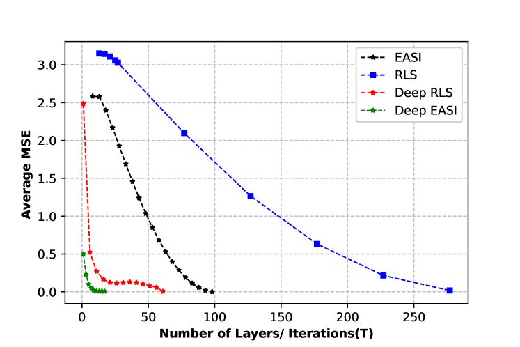
Figure 1: The average MSE of recovering $m=3$ source signals from $l=3$ observations using the Deep-RLS network, RLS [15] with $\beta=0.99$, EASI [10] and Deep-EASI vs. the number of layers/iterations $T$, when trained by MSE loss for $N=100$ epochs with a learning rate of $10^{-4}$.

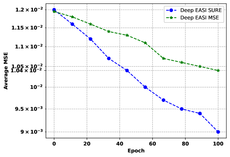
Figure 2: The performance of Deep EASI trained with MSE in (25) in comparison with SURE loss function in (29) .

V Conclusion

In this paper, we introduced two deep unrolling-based frameworks for adaptive filtering and demonstrated that the unrolled networks, trained as recursive neural networks, outperform their baseline counterparts. Moreover, we incorporated Stein’s unbiased risk estimator as a surrogate loss function for training the deep architectures which introduced further improvement in estimating the source signals.

VI Appendix: The RLS Recursive Formula

Let $\mathbf{A}$, $\mathbf{B}$, and $\mathbf{D}$ be positive definite matrices such that $\mathbf{A}=\mathbf{B}^{-1}+\mathbf{cD}^{-1}\mathbf{c}^{\top}.$ Using the matrix inversion lemma, the inverse of $\mathbf{A}$ can be expressed as

$$\mathbf{A}^{-1}=\mathbf{B}-\mathbf{Bc}(\mathbf{D}+\mathbf{c}^{T}\mathbf{Bc})^{-1}\mathbf{c}^{T}\mathbf{B}.$$ (32)

Now, assuming that the auto-correlation matrix $\mathbf{C_{y}}(t)$ is positive definite (and thus non-singular), by choosing $\mathbf{A=C_{y}}(t)$, $\mathbf{B}^{-1}=\beta\mathbf{C_{y}}(t-1)$, $\mathbf{c}=\mathbf{y}(t),\mathbf{D}^{-1}=\mathbf{I}$, one can compute $\mathbf{G}(t)=\mathbf{C_{y}}^{-1}(t)$ as proposed in (10).

VII Acknowledgement

The authors would like to express gratitude to Dr. Shahin Khobahi for his help with developing the ideas in a preliminary version of this manuscript, currently available on arXiv [19].

References

- [1] J. R. Hershey, J. L. Roux, and F. Weninger, “Deep unfolding: Model-based inspiration of novel deep architectures,” arXiv preprint arXiv:1409.2574, 2014.
- [2] V. Monga, Y. Li, and Y. C. Eldar, “Algorithm unrolling: Interpretable, efficient deep learning for signal and image processing,” arXiv preprint arXiv:1912.10557, 2019.
- [3] N. Shlezinger, Y. C. Eldar, and S. P. Boyd, “Model-based deep learning: On the intersection of deep learning and optimization,” IEEE Access, vol. 10, pp. 115 384–115 398, 2022.
- [4] Y. Zeng, S. Khobahi, and M. Soltanalian, “One-bit compressive sensing: Can we go deep and blind?” IEEE Signal Processing Letters, vol. 29, pp. 1629–1633, 2022.
- [5] S. Khobahi, N. Shlezinger, M. Soltanalian, and Y. C. Eldar, “LoRD-Net: Unfolded deep detection network with low-resolution receivers,” IEEE Transactions on Signal Processing, vol. 69, pp. 5651–5664, 2021.
- [6] V. Edupuganti, M. Mardani, S. Vasanawala, and J. Pauly, “Uncertainty quantification in deep MRI reconstruction,” IEEE Transactions on Medical Imaging, vol. 40, no. 1, pp. 239–250, 2021.
- [7] C. A. Metzler, A. Mousavi, R. Heckel, and R. G. Baraniuk, “Unsupervised learning with Stein’s unbiased risk estimator,” arXiv preprint arXiv:1805.10531, 2018.
- [8] M. Mardani, Q. Sun, V. Papyan, S. Vasanawala, J. Pauly, and D. Donoho, “Degrees of freedom analysis of unrolled neural networks,” arXiv preprint arXiv:1906.03742, 2019.
- [9] F. Shamshad, M. Awais, M. Asim, M. Umair, A. Ahmed et al., “Leveraging deep Stein’s unbiased risk estimator for unsupervised X-ray denoising,” arXiv preprint arXiv:1811.12488, 2018.
- [10] J.-F. Cardoso and B. H. Laheld, “Equivariant adaptive source separation,” IEEE Transactions on signal processing, vol. 44, no. 12, pp. 3017–3030, 1996.
- [11] J. M. T. Romano, R. Attux, C. C. Cavalcante, and R. Suyama, Unsupervised signal processing: channel equalization and source separation. CRC Press, 2018.
- [12] P. Pajunen and J. Karhunen, “Least-squares methods for blind source separation based on nonlinear PCA,” International Journal of Neural Systems, vol. 8, no. 05n06, pp. 601–612, 1997.
- [13] J. Karhunen, E. Oja, L. Wang, R. Vigario, and J. Joutsensalo, “A class of neural networks for independent component analysis,” IEEE Transactions on neural networks, vol. 8, no. 3, pp. 486–504, 1997.
- [14] B. Yang, “Projection approximation subspace tracking,” IEEE Transactions on Signal processing, vol. 43, no. 1, pp. 95–107, 1995.
- [15] J. Karhunen and P. Pajunen, “Blind source separation using least-squares type adaptive algorithms,” in IEEE International Conference on Acoustics, Speech, and Signal Processing, vol. 4, 1997, pp. 3361–3364.
- [16] L. Peng, C. Kümmerle, and R. Vidal, “On the convergence of IRLS and its variants in outlier-robust estimation,” in Proceedings of the IEEE/CVF Conference on Computer Vision and Pattern Recognition, June 2023, pp. 17 808–17 818.
- [17] S. Haykin and S. Haykin, Adaptive Filter Theory. Pearson, 2014.
- [18] A. F. Ajirlou and I. Partin-Vaisband, “A machine learning pipeline stage for adaptive frequency adjustment,” IEEE Transactions on Computers, vol. 71, no. 3, pp. 587–598, 2021.
- [19] Z. Esmaeilbeig, S. Khobahi, and M. Soltanalian, “Deep-RLS: A model-inspired deep learning approach to nonlinear PCA,” arXiv e-prints, pp. arXiv–2011, 2020.
- [20] A. Paszke, S. Gross, F. Massa, A. Lerer, J. Bradbury, G. Chanan, T. Killeen, Z. Lin, N. Gimelshein, L. Antiga, A. Desmaison, A. Kopf, E. Yang, Z. DeVito, M. Raison, A. Tejani, S. Chilamkurthy, B. Steiner, L. Fang, J. Bai, and S. Chintala, “Pytorch: An imperative style, high-performance deep learning library.” Curran Associates, Inc., 2019, pp. 8024–8035.
- [21] C. M. Stein, “Estimation of the mean of a multivariate normal distribution,” The annals of Statistics, pp. 1135–1151, 1981.
- [22] Y. C. Eldar, “Generalized SURE for exponential families: Applications to regularization,” IEEE Transactions on Signal Processing, vol. 57, no. 2, pp. 471–481, 2008.
- [23] P. Nobel, E. Candès, and S. Boyd, “Tractable evaluation of Stein’s unbiased risk estimator with convex regularizers,” arXiv preprint arXiv:2211.05947, 2022.
- [24] D. P. Kingma and J. Ba, “Adam: A method for stochastic optimization,” arXiv preprint arXiv:1412.6980, 2014.