Continuous-Time Distributed Dynamic Programming for Networked Multi-Agent Markov Decision Processes

Abstract

The main goal of this paper is to investigate continuous-time distributed dynamic programming (DP) algorithms for networked multi-agent Markov decision problems (MAMDPs). In our study, we adopt a distributed multi-agent framework where individual agents have access only to their own rewards, lacking insights into the rewards of other agents. Moreover, each agent has the ability to share its parameters with neighboring agents through a communication network, represented by a graph. We first introduce a novel distributed DP, inspired by the distributed optimization method of Wang and Elia. Next, a new distributed DP is introduced through a decoupling process. The convergence of the DP algorithms is proved through systems and control perspectives. The study in this paper sets the stage for new distributed temporal different learning algorithms.

I Introduction

A Markov decision problem (MDP)[1, 2] is a sequential decision-making problem that aims to find an optimal policy in dynamic environments. Multi-agent MDPs (MAMDPs)[3, 4] extend the MDP framework to include multiple agents interacting with one another. These agents can either cooperate toward a shared goal or compete for individual objectives. In this study, we focus primarily on the cooperative scenario.

In MAMDPs, full information about the environment, such as the global state, action, and reward, is often unavailable to each agent. This lack of complete information can arise for a variety of reasons, including sensor or infrastructure limitations, privacy and security concerns, and computational constraints, among others. As a result, various information structures are adopted based on the specific application. One notable instance is the centralized MAMDP, where every agent has access to complete information. In contrast, in distributed MAMDPs, agents may only have access to local data about the global state, action, and rewards. Sometimes, agents can share information with each other via communication networks, an environment termed as the networked MAMDP.

In this paper, we investigate new continuous-time distributed DP algorithms for a networked MAMDP. In this setting, agents can share their local parameters with their neighbors over a communication network described by a graph, $\mathcal{G}$. The proposed algorithms are distributed in the sense that only local rewards, $r_{i}$, are given to each agent. Meanwhile, the global reward is a sum or an average of the local rewards, i.e., $r=(r_{1}+r_{2}+\cdots+r_{N})/N$, where $N$ is the total number of agents. To address the MAMDP in a distributed manner, we employ the distributed optimization techniques [5, 6, 7, 8]. These techniques enable multiple agents to calculate a common solution through parameter mixing (or averaging) steps with their neighbors.

In particular, we introduce two novel continuous-time distributed DP [9] algorithms. The first algorithm is inspired by the distributed optimization technique of Wang and Elia [10]. The second DP algorithm is developed through a special decoupling process. The convergence of these algorithms is proved from systems and control perspectives [11].

The main contributions of this paper are summarized as follows: To the authors’ best knowledge, the algorithms presented in this paper are the first attempts to develop and analyze distributed DP algorithms characterized by simple continuous-time linear dynamics. These algorithms are readily analyzable from a control theory standpoint. This approach, based on systems and control theory, simplifies and clarifies the analysis, especially for those with a background in control theory, and provides additional insights into the distributed DP. Moreover, this paper establishes a foundation for developing new distributed temporal difference learning algorithms.

While numerous studies [12, 13, 14, 15, 16, 17, 18, 19, 20] have studied model-free distributed temporal difference learning algorithms under a variety of scenarios and conditions, this paper is among the first to thoroughly investigate model-based continuous-time linear dynamics. Although model-free methods are generally more applicable in a broader range of situations, the approaches in this paper can be readily extended to model-free temporal difference learning techniques.

II Preliminaries

II-A Notation and terminology

The following notation is adopted: ${\mathbb{R}}^{n}$ denotes the $n$-dimensional Euclidean space; ${\mathbb{R}}^{n\times m}$ denotes the set of all $n\times m$ real matrices; ${\mathbb{R}}_{+}$ and ${\mathbb{R}}_{++}$ denote the sets of nonnegative and positive real numbers, respectively, $A^{T}$ denotes the transpose of matrix $A$; $I_{n}$ denotes the $n\times n$ identity matrix; $I$ denotes the identity matrix with appropriate dimension; $\|\cdot\|_{2}$ denotes the standard Euclidean norm; $\|x\|_{D}:=\sqrt{x^{T}Dx}$ for any positive-definite $D$; $\lambda_{\min}(A)$ denotes the minimum eigenvalue of $A$ for any symmetric matrix $A$; $|{\mathcal{S}}|$ denotes the cardinality of the set for any finite set ${\mathcal{S}}$; $[x]_{i}$ is the $i$-th element for any vector $x$; $[P]_{ij}$ indicates the element in $i$-th row and $j$-th column for any matrix $P$; if ${\bf z}$ is a discrete random variable which has $n$ values and $\mu\in{\mathbb{R}}^{n}$ is a stochastic vector, then ${\bf z}\sim\mu$ stands for ${\mathbb{P}}[{\bf z}=i]=[\mu]_{i}$ for all $i\in\{1,\ldots,n\}$; ${\bf 1}_{n}\in{\mathbb{R}}^{n}$ denotes an $n$-dimensional vector with all entries equal to one.

II-B Graph theory

An undirected graph with the node set ${\mathcal{V}}$ and the edge set ${\mathcal{E}}\subseteq{\mathcal{V}}\times{\mathcal{V}}$ is denoted by ${\mathcal{G}}=({\mathcal{E}},{\mathcal{V}})$. We define the neighbor set of node $i$ as ${\mathcal{N}}_{i}:=\{j\in{\mathcal{V}}:(i,j)\in{\mathcal{E}}\}$. The adjacency matrix of $\mathcal{G}$ is defined as a matrix $W$ with $[W]_{ij}=1$, if and only if $(i,j)\in{\mathcal{E}}$. If $\mathcal{G}$ is undirected, then $W=W^{T}$. A graph is connected, if there is a path between any pair of vertices. The graph Laplacian is $L=H-W$, where $H$ is a diagonal matrix with $[H]_{ii}=|{\mathcal{N}}_{i}|$. If the graph is undirected, then $L$ is symmetric positive semi-definite. It holds that $L{\bf 1}_{|{\mathcal{V}}|}=0$. If ${\mathcal{G}}$ is connected, $0$ is a simple eigenvalue of $L$, i.e., ${\bf 1}_{|{\mathcal{V}}|}$ is the unique eigenvector corresponding to $0$, and the span of ${\bf 1}_{|{\mathcal{V}}|}$ is the null space of $L$.

II-C Markov decision process

A Markov decision process (MDP) [1] is characterized by a quadruple ${\mathcal{M}}:=({\mathcal{S}},{\mathcal{A}},P,r,\gamma)$, where ${\mathcal{S}}$ is a finite state space (observations in general), $\mathcal{A}$ is a finite action space, $P(s,a,s^{\prime})$ represents the (unknown) state transition probability from state $s$ to $s^{\prime}$ given action $a$, $r:{\mathcal{S}}\times{\mathcal{A}}\times{\mathcal{S}}$ is the reward function, and $\gamma\in(0,1)$ is the discount factor. In particular, if action $a$ is selected with the current state $s$, then the state transits to $s^{\prime}$ with probability $P(s,a,s^{\prime})$ and incurs a random reward $r(s,a,s^{\prime})$. The stochastic policy is a map $\pi:{\mathcal{S}}\times{\mathcal{A}}\to[0,1]$ representing the probability $\pi(a|s)$ of taking action $a$ at the current state $s$, $P^{\pi}$ denotes the transition matrix, and $d:{\mathcal{S}}\to{\mathbb{R}}$ denotes the stationary distribution of the state $s\in{\mathcal{S}}$ under the policy $\pi$. We also define $R^{\pi}(s)$ as the expected reward given the policy $\pi$ and the current state $s$. The infinite-horizon discounted value function with policy $\pi$ is

$$J^{\pi}(s):={\mathbb{E}}\left[\left.\sum_{k=0}^{\infty}{\gamma^{k}r(s_{k},a_{k},s_{k+1})}\right|s_{0}=s\right],$$

where ${\mathbb{E}}$ stands for the expectation taken with respect to the state-action trajectories following the state transition $P^{\pi}$. Given pre-selected basis (or feature) functions $\phi_{1},\ldots,\phi_{q}:{\mathcal{S}}\to{\mathbb{R}}$, $\Phi\in{\mathbb{R}}^{|{\mathcal{S}}|\times q}$ is defined as a full column rank matrix whose $s$-th row vector is $\phi(s):=\begin{bmatrix}\phi_{1}(s)&\cdots&\phi_{q}(s)\end{bmatrix}$. The goal of the Markov decision problem with the linear function approximation is to find the weight vector $\theta$ such that $J_{\theta}:=\Phi\theta$ approximates the true value function $J^{\pi}$. This is typically done by minimizing the mean-square projected Bellman error loss function [21]

$${\min_{\theta\in{\mathbb{R}}^{q}}}{\rm{MSPBE}}(\theta):={\min_{\theta\in{\mathbb{R}}^{q}}}\frac{1}{2}\left\|{\Pi({R^{\pi}}+\gamma{P^{\pi}}\Phi\theta-\Phi\theta)}\right\|_{D}^{2},$$ (1)

where $D$ is a diagonal matrix with positive diagonal elements $d(s),s\in{\mathcal{S}}$, $\Pi$ is the projection onto the range space of $\Phi$, denoted by $R(\Phi)$: $\Pi(x):=\operatorname{arg\,min}_{x}\|x-x^{\prime}\|_{D}^{2}$, $x^{\prime}\in R(\Phi)$, and $R^{\pi}\in{\mathbb{R}}^{|{\mathcal{S}}|}$ is a vector enumerating all $R^{\pi}(s),s\in{\mathcal{S}}$. The projection can be performed by the matrix multiplication: we write $\Pi(x):=\Pi x$, where $\Pi:=\Phi(\Phi^{T}D\Phi)^{-1}\Phi^{T}D$. The solutions of (1) is known to be equivalent to those of the so-called projected Bellman equation

$$\Phi\theta=\Pi(R^{\pi}+\gamma P^{\pi}\Phi\theta),$$ (2)

whose solution is given by

$$\theta^{*}=-(\Phi^{T}D(\gamma P^{\pi}-I)\Phi)^{-1}\Phi^{T}DR^{\pi}.$$ (3)

III Multi-agent MDP

In this section, we introduce the notion of the distributed MAMDP, which will be studied throughout the paper. Consider $N$ agents labeled by $i\in\{1,\ldots,N\}=:{\mathcal{V}}$. A multi-agent Markov decision process is characterized by $({\mathcal{S}},\{{\mathcal{A}}_{i}\}_{i\in{\mathcal{V}}},P,\{r_{i}\}_{i\in{\mathcal{V}}},\gamma)$, where $\gamma\in(0,1)$ is the discount factor, ${\mathcal{S}}$ is a finite state space, ${\mathcal{A}}_{i}$ is a finite action space of agent $i$, $a:=(a_{1},\ldots,a_{N})$ is the joint action, ${\mathcal{A}}:=\prod_{i=1}^{N}{{\mathcal{A}}_{i}}$ is the corresponding joint action space, $r_{i}:{\mathcal{S}}\times{\mathcal{A}}\times{\mathcal{S}}\to{\mathbb{R}}$ is a reward function of agent $i$, and $P(s,a,s^{\prime})$ represents the transition model of the state $s$ with the joint action $a$ and the corresponding joint action space ${\mathcal{A}}$. The stochastic policy of agent $i$ is a mapping $\pi_{i}:{\mathcal{S}}\times{\mathcal{A}}_{i}\to[0,1]$ representing the probability $\pi_{i}(a_{i}|s)$ of selecting action $a_{i}$ at the state $s$, and the corresponding joint policy is $\pi(a|s):=\prod_{i=1}^{N}{\pi_{i}(a_{i}|s)}$. Moreover, $P^{\pi}$ denotes the transition matrix, and $d:{\mathcal{S}}\to{\mathbb{R}}$ denotes the stationary state distribution under the joint policy $\pi$. In particular, if the joint action $a$ is selected with the current state $s$, then the state transits to $s^{\prime}$ with probability $P(s,a,s^{\prime})$, and each agent $i$ observes a reward $r_{i}(s,a,s^{\prime})$. In addition, $J^{\pi}$ is the infinite-horizon discounted value function with policy $\pi$ and reward $r=(r_{1}+\cdots+r_{N})/N$ satisfying $J^{\pi}=\frac{1}{N}\sum_{i=1}^{N}{R_{i}^{\pi}}+\gamma P^{\pi}J^{\pi}$.

Problem 1 (Distributed value evaluation problem)

The goal of each agent $i$ is to find the value function of the centralized reward $r=(r_{1}+\cdots+r_{N})/N$, where only the local reward $r_{i}$ is given to each agent, and parameters can be shared with its neighbors over communication network represented by the graph $\cal G$.

In this paper, we assume that each agent does not have access to the rewards of the other agents. For instance, there is no centralized coordinator; thus, each agent is unaware of the rewards of other agents. On the other hand, we suppose that each agent knows only the parameters of adjacent agents over the network graph, assuming that the agents can communicate with each other. Without each agent knowing the full reward algorithm of the group, our algorithm produces the same result as if each agent were receiving the average rewards of the group.

IV Continuous-time distributed dynamic programming

For the sake of notational simplicity in representing a multi-agent environment, we first introduce the stacked vector and matrix notations:

$$\bar{\theta}:=\begin{bmatrix}\theta_{1}\\ \vdots\\ \theta_{N}\\ \end{bmatrix},\quad\bar{R}^{\pi}:=\begin{bmatrix}R_{1}^{\pi}\\ \vdots\\ R_{N}^{\pi}\\ \end{bmatrix},$$

$$\bar{P}^{\pi}:=I_{N}\otimes P^{\pi},\quad\bar{L}:=L\otimes I_{q},\quad\bar{D}:=I_{N}\otimes D,$$

$$\bar{\Phi}:=I_{N}\otimes\Phi$$

Before delving into the distributed dynamic programming (DP), it is beneficial to examine the centralized version of DP. This provides a foundation that can be extended to the distributed version. The centralized variant can be naturally derived from the solution of the MSPBE for a single agent, as shown in (3).

IV-A Centralized dynamic programming

In the centralized multi-agent case, the same reward $R_{c}^{\pi}=(R_{1}^{\pi}+\cdots+R_{N}^{\pi})/N$ for every agent is given. Then, it can be simply considered as the single agent case with stacked vector and matrix notation. According to the single-agent MDP results in (3), the optimal solution is given as

$${\bar{\theta}^{*}}:=-{({\bar{\Phi}^{T}}\bar{D}(\gamma{\bar{P}^{\pi}}-I)\bar{\Phi})^{-1}}{\bar{\Phi}^{T}}\bar{D}({\bf{1}}_{N}\otimes R_{c}^{\pi}),$$ (4)

which minimizes the corresponding MSPBE (1). Using algebraic manipulations, we can easily prove that $\bar{\theta}^{*}$ can be represented by $\bar{\theta}^{*}={\bf{1}}_{N}\otimes\theta_{\infty}^{c}$, where

$$\theta_{\infty}^{c}:=-(\Phi^{T}D(-I+\gamma P^{\pi})\Phi)^{-1}\Phi^{T}DR_{c}^{\pi}.$$ (5)

The solution can be found using a standard DP method [9]. In this paper, we will consider a DP in the continuous-time domain (or ODE) as follows:

$$\frac{d}{dt}\bar{\theta}_{t}=\bar{\Phi}^{T}\bar{D}(-I+\gamma\bar{P}^{\pi})\bar{\Phi}\bar{\theta}_{t}+\bar{\Phi}^{T}\bar{D}({\bf{1}}_{N}\otimes R_{c}^{\pi}),$$ (6)

which is a linear ODE. We can easily prove that $\bar{\theta}^{*}$ is an asymptotically stable equilibrium point.

Proposition 1

$\bar{\theta}^{*}$ is a unique asymptotically stable equilibrium point of the linear system in (6), i.e., $\bar{\theta}_{t}\to\bar{\theta}^{*}$ as $t\to\infty$.

Proof:

Using $\bar{\Phi}^{T}\bar{D}(\gamma\bar{P}^{\pi}-I)\bar{\Phi}\bar{\theta}^{*}+\bar{\Phi}^{T}\bar{D}\bar{R}^{\pi}=0$, (6) can be represented by the linear system

$$\frac{d}{dt}(\bar{\theta}_{t}-\bar{\theta}^{*})=\bar{\Phi}^{T}\bar{D}(-I+\gamma\bar{P}^{\pi})\bar{\Phi}(\bar{\theta}_{t}-\bar{\theta}^{*}).$$

We can easily prove that $\bar{\Phi}^{T}\bar{D}(-I+\gamma\bar{P}^{\pi})\bar{\Phi}$ is negative definite, and hence, Hurwitz [22, pp. 209]. Therefore, $\bar{\theta}_{t}-\bar{\theta}^{*}\to 0$ as $t\to\infty$, which completes the proof. ∎

To solve (6), we must assume that the central reward $R_{c}^{\pi}$ is accessible to all agents. In subsequent sections, we will explore distributed versions where only the local reward $R^{\pi}_{i}$ is provided to each agent $i$. We present two versions: the first is inspired by [10], while the second is a novel approach that offers more desirable properties compared to the first when integrated into reinforcement learning (RL) frameworks [23].

IV-B Distributed dynamic programming version 1

In the networked multi-agent setting, each agent receives each of their local rewards, and parameters from neighbors over a communication graph. Based on the ideas of Wang and Elia in [10], we can convert the continuous-time ODE in (6) into

$$\frac{d}{dt}\bar{\theta}_{t} =\bar{\Phi}^{T}\bar{D}(-I+\gamma\bar{P}^{\pi})\bar{\Phi}\bar{\theta}_{t}+\bar{\Phi}^{T}\bar{D}\bar{R}^{\pi}-\bar{L}\bar{\theta}_{t}-\bar{L}\bar{w}_{t},$$

$$\frac{d}{dt}\bar{w}_{t} =\bar{L}\bar{\theta}_{t}.$$ (7)

Compared to (6), the above ODE consists of an auxiliary vector $\bar{w}_{t}$ and the graph Laplacian matrix $\bar{L}$. Here, the Laplacian helps the consensus of each agent, and the auxiliary vector potentially allows agents make better use of their local information. Note that each agent only uses local information by multiplying the Laplacian in both equations. The ODE in (7) can be written as Algorithm 1 from a local view.

Algorithm 1 Distributed dynamic programming version 1

1:Initialize $\theta_{0}^{i},w_{0}^{i},i\in\{1,2,\ldots,N\}$.

2:for $t\geq 0$ do

3:     for agent $i\in\{1,\ldots,N\}$ do

4:         Update

$$\frac{d}{dt}\theta_{t}^{i} =\Phi^{T}D(-I+\gamma P^{\pi})\Phi\theta_{t}^{i}+\Phi^{T}DR_{i}^{\pi}$$

$$-\left(|{\cal N}_{i}|{\theta_{t}^{i}}-\sum_{j\in{\cal N}_{i}}{\theta_{t}^{j}}\right)-\left(|{\cal N}_{i}|w_{t}^{i}-\sum_{j\in{\cal N}_{i}}{w_{t}^{j}}\right)$$

$$\frac{d}{dt}w_{t}^{i} =|{\cal N}_{i}|\theta_{t}^{i}-\sum_{j\in{\cal N}_{i}}{\theta_{t}^{j}}$$

where ${\mathcal{N}}_{i}$ is the neighborhood of node $i$ on the graph ${\mathcal{G}}$.

5:     end for

6:end for

As can be seen from Algorithm 1, each agent $i$ updates its local parameter $\theta_{t}^{i}$ using its own reward $R_{i}^{\pi}$ and parameters of its neighbors $\theta_{t}^{j},j\in{\cal N}_{i}$. Nevertheless, we can prove that each agent $i$ can find the global solution $\theta_{\infty}^{c}$ given in (5). To this end, we first provide stationary points of this system in the next result, and then prove that both weight vector $\bar{\theta}_{t}$ and auxiliary vector $\bar{w}_{t}$ reach the stationary point.

Proposition 2 (Equilibrium points)

The unique equilibrium point, $\bar{\theta}_{\infty}$, of the linear system in (7) corresponding to the vector $\bar{\theta}_{t}$ is given by $\bar{\theta}^{*}={\bf{1}}_{N}\otimes\theta_{\infty}^{c}$, where $\theta_{\infty}^{c}$ is defined in (5). Moreover, for the auxiliary vectors $\bar{w}_{t}$, the corresponding equilibrium points are all solutions, $\bar{w}_{\infty}$, of the following linear equation:

$$\bar{L}\bar{w}_{\infty}=\begin{bmatrix}\Phi^{T}D\left(R_{1}^{\pi}-\frac{1}{N}\sum_{i=1}^{N}{R_{i}^{\pi}}\right)\\ \Phi^{T}D\left(R_{2}^{\pi}-\frac{1}{N}\sum_{i=1}^{N}{R_{i}^{\pi}}\right)\\ \vdots\\ \Phi^{T}D\left(R_{N}^{\pi}-\frac{1}{N}\sum_{i=1}^{N}{R_{i}^{\pi}}\right)\\ \end{bmatrix}.$$ (8)

The proof of Proposition 2 is given in Appendix VI-A. Proposition 2 implies that the local parameter $\theta^{i}_{t}$ reaches a consensus, i.e.,

$$\lim_{t\to\infty}\theta_{t}^{1}=\lim_{t\to\infty}\theta_{t}^{2}=\cdots=\lim_{t\to\infty}\theta_{t}^{N}=\theta_{\infty}^{c}.$$

On the other hand, $\bar{w}_{\infty}$ lies in an affine subspace, which is infinite. Next, we prove global asymptotic stability of the equilibrium points, whose proof is given in Appendix VI-B.

Proposition 3 (Global asymptotic stability)

The equilibrium points $(\bar{\theta}_{\infty},\bar{w}_{\infty})$ of (7) is globally asymptotically stable, i.e., $\bar{\theta}_{t}\to\bar{\theta}_{\infty}=\bar{\theta}^{*}$ and $\bar{w}_{t}\to\bar{w}_{\infty}$ as $t\to\infty$.

Proposition 3 establishes that the first DP version converges to the solution $\bar{\theta}^{*}$. As a potential application, it is easy to envision the development of a distributed RL by replacing certain terms in Algorithm 1 with sample transitions of the underlying MDP. In such a scenario, the asymptotic stability of the continuous-time DP in Algorithm 1 could be leveraged to demonstrate the convergence of the RL, using the well-established Borkar-Meyn theorem [24]. A primary challenge in applying the Borkar-Meyn theorem is the non-uniqueness of the equilibrium point of the ODE in (7). For the Borkar-Meyn theorem’s application, the existence of a unique equilibrium point is a prerequisite. As such, the stability analysis for Algorithm 1 cannot be directly converted to its RL counterpart. In the following subsection, we introduce the second version, which can potentially address the aforementioned challenges.

IV-C Distributed dynamic programming version 2

Motivated by the aforementioned discussion, we propose the following continuous-time DP:

$$\frac{d}{dt}\bar{\theta}_{t} =\bar{\Phi}^{T}\bar{D}(-I+\gamma\bar{P}^{\pi})\bar{\Phi}\bar{\theta}_{t}+\bar{\Phi}^{T}\bar{D}\bar{R}^{\pi}-\bar{L}\bar{\theta}_{t}$$

$$\frac{d}{dt}\bar{w}_{t} =\bar{\theta}_{t}-\bar{w}_{t}-\bar{L}\bar{w}_{t}-\bar{L}\bar{v}_{t}$$

$$\frac{d}{dt}\bar{v}_{t} =\bar{L}\bar{w}_{t}$$ (9)

Algorithm 2 Distributed dynamic programming version 2

1:Initialize $\theta_{0}^{i},w_{0}^{i},i\in\{1,2,\ldots,N\}$.

2:for $t\geq 0$ do

3:     for agent $i\in\{1,\ldots,N\}$ do

4:         Update

$$\begin{split}\frac{d}{dt}\theta_{t}^{i}&=\Phi^{T}D(-I+\gamma P^{\pi})\Phi\theta_{t}^{i}+\Phi^{T}DR_{i}^{\pi}\\ &-\left(|{\mathcal{N}}_{i}|\theta_{t}^{i}-\sum_{j\in{\mathcal{N}}_{i}}{\theta_{t}^{j}}\right)\end{split}$$

$$\begin{split}\frac{d}{dt}w_{t}^{i}&=\theta_{t}^{i}-w_{t}^{i}\\ &-\left(|{\mathcal{N}}_{i}|w_{t}^{i}-\sum_{j\in{\mathcal{N}}_{i}}{w_{t}^{j}}\right)-\left(|{\mathcal{N}}_{i}|v_{t}^{i}-\sum_{j\in{\mathcal{N}}_{i}}{v_{t}^{j}}\right)\end{split}$$

$$\begin{split}\frac{d}{dt}v_{t}^{i}{}&=|{\mathcal{N}}_{i}|w_{t}^{i}-\sum_{j\in{\mathcal{N}}_{i}}{w_{t}^{j}}\end{split}$$

where ${\mathcal{N}}_{i}$ is the neighborhood of node $i$ on the graph ${\mathcal{G}}$.

5:     end for

6:end for

The overall algorithm, when viewed locally, is summarized in Algorithm 2. We can demonstrate that $\bar{w}_{t}\to\bar{\theta}^{*}$ as $t\to\infty$, where $\bar{\theta}^{*}$ is defined in (4). Thus, this DP can serve as an alternative to the DP in (7). A key distinction between the current DP and its predecessor is the decoupling of the ODE corresponding to $\bar{\theta}_{t}$ from the components linked to $(\bar{w}_{t},\bar{v}_{t})$ The ODE for $\bar{\theta}_{t}$ can be seen as the local value function estimation, while the ODE for $(\bar{w}_{t},\bar{v}_{t})$ represents the parameter mixing component. This characteristic renders it more apt for RL applications. We will first establish the equilibrium points of (9) and their asymptotic stability.

Proposition 4 (Equilibrium points)

The unique equilibrium point, $\bar{w}_{\infty}$, of the linear system in (9) corresponding to the vector $\bar{w}_{t}$ is given by $\bar{w}_{\infty}={\bf{1}}_{N}\otimes\theta_{\infty}^{c}=\bar{\theta}^{*}$, where $\theta_{\infty}^{c}$ is defined in (5). Moreover, for the vector $\bar{\theta}_{t}$, the corresponding equilibrium points, $\bar{\theta}_{\infty}$, are all solutions of the following linear equation:

$$\frac{1}{N}\sum_{i=1}^{N}{\theta_{\infty}^{i}}=-(\Phi^{T}D(-I+\gamma P^{\pi})\Phi)^{-1}\Phi^{T}D\left(\frac{1}{N}\sum_{i=1}^{N}{R_{i}^{\pi}}\right)$$ (10)

For another vector $\bar{v}_{t}$, the corresponding equilibrium points, $\bar{v}_{\infty}$, are all solutions of the following linear equation:

$$\bar{L}\bar{v}_{\infty}=\bar{\theta}_{\infty}-\bar{w}_{\infty}.$$ (11)

The proof of Proposition 4 is given in Appendix VI-C. Next, we establish the global asymptotic stability of (9), whose proof is given in Appendix VI-D.

Proposition 5 (Global asymptotic stability)

The equilibrium points $(\bar{\theta}_{\infty},\bar{w}_{\infty},\bar{v}_{\infty})$ of (9) is globally asymptotically stable, i.e., $\bar{\theta}_{t}\to\bar{\theta}_{\infty}$, $\bar{w}_{t}\to\bar{w}_{\infty}=\bar{\theta}^{*}$, and $\bar{v}_{t}\to\bar{v}_{\infty}$ as $t\to\infty$.

Example 1

Let us consider the Markov decision process borrowed from [20] with

$$P^{\pi}=\begin{bmatrix}0.1&0.5&0.2&0.2\\ 0.5&0.0&0.1&0.4\\ 0.0&0.9&0.1&0.0\\ 0.2&0.1&0.1&0.6\\ \end{bmatrix},$$

where $\pi$ is not explicitly specified, $|{\mathcal{S}}|=4$, $\gamma=0.8$, and the local expected reward functions

$$R_{1}^{\pi}=\begin{bmatrix}0&0&0&50\\ \end{bmatrix}^{T},\quad R_{2}^{\pi}=\begin{bmatrix}0&0&0&0\\ \end{bmatrix}^{T},$$

$$R_{3}^{\pi}=\begin{bmatrix}0&0&0&0\\ \end{bmatrix}^{T},\quad R_{4}^{\pi}=\begin{bmatrix}0&0&0&0\\ \end{bmatrix}^{T},$$

$$R_{5}^{\pi}=\begin{bmatrix}0&0&0&0\\ \end{bmatrix}^{T},$$

The feature matrix is

$$\Phi=\left[{\begin{array}[]{*{20}{c}}1&0\\ 1&0\\ 0&2\\ 0&2\end{array}}\right]$$

and the five RL agents over the network given in Figure 1.

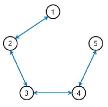
Figure 1: Network topology of five RL agents.

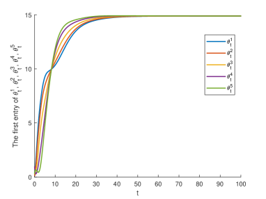
Figure 2: Algorithm 1: Evolution of the first entries of $\theta_{t}^{1}$, $\theta_{t}^{2}$, $\theta_{t}^{3}$, $\theta_{t}^{4}$, and $\theta_{t}^{5}$.

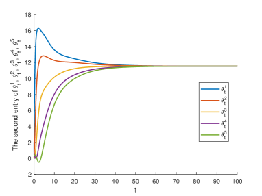
Figure 3: Algorithm 1: Evolution of the second entries of $\theta_{t}^{1}$, $\theta_{t}^{2}$, $\theta_{t}^{3}$, $\theta_{t}^{4}$, and $\theta_{t}^{5}$.

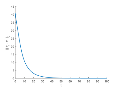
Figure 4: Algorithm 1: Evolution of ${\left\|{{{\bar{\theta}}_{t}}-{{\bar{\theta}}^{*}}}\right\|_{2}}$.

For Algorithm 1, Figure 2 depicts the evolutions of the first entries of $\theta_{t}^{1}$, $\theta_{t}^{2}$, $\theta_{t}^{3}$, and $\theta_{t}^{4}$. Similarly, Figure 3 illustrates the evolutions of the first entries of $\theta_{t}^{1}$, $\theta_{t}^{2}$, $\theta_{t}^{3}$, and $\theta_{t}^{4}$. These results demonstrate that the parameters of the five agents reach a consensus. Figure 4 shows the evolution of the error $\|{{{\bar{\theta}}_{t}}-{{\bar{\theta}}^{*}}}\|_{2}$, and empirically proves that the parameter of the agents ${\bar{\theta}}_{t}$ converges to the optimal solution ${\bar{\theta}}^{*}$.

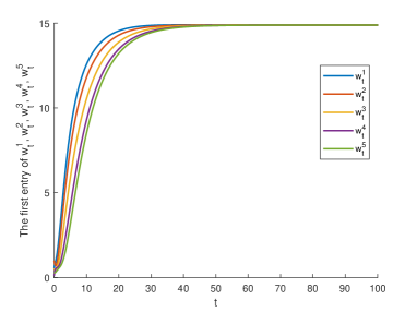
Figure 5: Algorithm 2: Evolution of the first entries of $w_{t}^{1}$, $w_{t}^{2}$, $w_{t}^{3}$, $w_{t}^{4}$, and $w_{t}^{5}$.

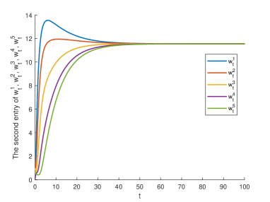
Figure 6: Algorithm 2: Evolution of the second entries of $w_{t}^{1}$, $w_{t}^{2}$, $w_{t}^{3}$, $w_{t}^{4}$, and $w_{t}^{5}$.

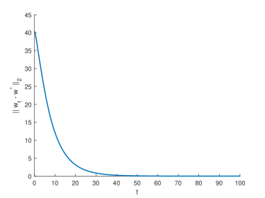
Figure 7: Algorithm 2: Evolution of ${\left\|{{{\bar{w}}_{t}}-{{\bar{\theta}}^{*}}}\right\|_{2}}$.

Next, Figure 5, Figure 6, Figure 7 give similar results corresponding to Algorithm 2. The results also empirically demonstrate the validity of the proposed Algorithm 2. We can also observe that both algorithms have similar convergence speeds.

V Conclusion

This paper introduces new continuous-time distributed DP algorithms for MAMDPs and establishes their convergence. These are the initial efforts to develop distributed DP algorithms with simple continuous-time linear dynamics. The development and analysis, based on in systems and control theory, allow for more intuitive analysis from a control theory perspective, and improve clarity particularly for people with backgrounds in systems and control. The results in this paper offer further insights into distributed DP algorithms. Furthermore, the paper sets a foundation for the development of new distributed temporal difference learning algorithms.

VI Appendix

VI-A Proof of Proposition 2

Let $(\bar{\theta}_{\infty},\bar{w}_{\infty})$ be an equilibrium point corresponding to $(\bar{\theta}_{t},\bar{w}_{t})$. Then, it should satisfy the following equation:

$$\bar{\Phi}^{T}\bar{D}(-I+\gamma\bar{P}^{\pi})\bar{\Phi}\bar{\theta}_{\infty}+\bar{\Phi}^{T}\bar{D}\bar{R}^{\pi}-\bar{L}\bar{\theta}_{\infty}-\bar{L}\bar{w}_{\infty} =0$$

$$\bar{L}\bar{\theta}_{\infty} =0.$$

The second equation implies $\bar{\theta}_{\infty}={\bf{1}}_{N}\otimes v$ for some $v\in{\mathbb{R}}^{q}$. Plugging this relation into the first equation, we have

$$\bar{\Phi}^{T}\bar{D}(-I+\gamma\bar{P}^{\pi})\bar{\Phi}\bar{\theta}_{\infty}+\bar{\Phi}^{T}\bar{D}\bar{R}^{\pi}-\bar{L}\bar{w}_{\infty}=0,$$ (12)

where we used $\bar{L}\bar{\theta}_{\infty}=0$. Multiplying $({\bf 1}_{N}\otimes I)^{T}$ from the left yields

$$({\bf 1}_{N}\otimes I)^{T}[\bar{\Phi}^{T}\bar{D}(-I+\gamma\bar{P}^{\pi})\bar{\Phi}\bar{\theta}_{\infty}+\bar{\Phi}^{T}\bar{D}\bar{R}^{\pi}]=0,$$

where we used $({\bf{1}}_{N}\otimes I)^{T}\bar{L}\bar{w}_{\infty}=0$. The equation can be equivalently written as

$$N\Phi^{T}D(-I+\gamma P^{\pi})\Phi v=-\sum_{i=1}^{N}{\Phi^{T}DR_{i}^{\pi}}$$

Since $\Phi^{T}D(-I+\gamma P^{\pi})\Phi$ is nonsingular from [22, pp. 209], it follows that

$$v=-(\Phi^{T}D(-I+\gamma P^{\pi})\Phi)^{-1}\Phi^{T}D\left(\frac{1}{N}\sum_{i=1}^{N}{R_{i}^{\pi}}\right),$$

which is identical to (5), i.e., $v=\theta_{\infty}^{c}$. Therefore, $\bar{\theta}_{\infty}^{c}={\bf{1}}_{N}\otimes v={\bf{1}}_{N}\otimes\theta_{\infty}^{c}=\bar{\theta}^{*}$. Plugging it back to (12) leads to (8). This completes the proof.

VI-B Proof of Proposition 3

With $\bar{\Phi}^{T}\bar{D}(-I+\gamma\bar{P}^{\pi})\bar{\Phi}\bar{\theta}_{\infty}+\bar{\Phi}^{T}\bar{D}\bar{R}^{\pi}-\bar{L}\bar{w}_{\infty}=0$ and $\bar{L}\bar{\theta}_{\infty}=0$, the ODEs in (7) become

$$\begin{split}\frac{d}{dt}(\bar{\theta}_{t}-\bar{\theta}_{\infty}){}&=\bar{\Phi}^{T}\bar{D}(-I+\gamma\bar{P}^{\pi})\bar{\Phi}(\bar{\theta}_{t}-\bar{\theta}_{\infty})\\ &-\bar{L}(\bar{\theta}_{t}-\bar{\theta}_{\infty})-\bar{L}(\bar{w}_{t}-\bar{w}_{\infty})\end{split}$$ (13)

$$\begin{split}\frac{d}{dt}(\bar{w}_{t}-\bar{w}_{\infty}){}&=\bar{L}(\bar{\theta}_{t}-\bar{\theta}_{\infty}).\end{split}$$

Consider the function

$$V\left(\begin{bmatrix}\bar{\theta}_{t}-\bar{\theta}_{\infty}\\ \bar{w}_{t}-\bar{w}_{\infty}\\ \end{bmatrix}\right)=\begin{bmatrix}\bar{\theta}_{t}-\bar{\theta}_{\infty}\\ \bar{w}_{t}-\bar{w}_{\infty}\\ \end{bmatrix}^{T}\begin{bmatrix}\bar{\theta}_{t}-\bar{\theta}_{\infty}\\ \bar{w}_{t}-\bar{w}_{\infty}\\ \end{bmatrix}.$$

Its time-derivative along the trajectory is

$$\dot{V}\left(\begin{bmatrix}\bar{\theta}_{t}-\bar{\theta}_{\infty}\\ \bar{w}_{t}-\bar{w}_{\infty}\\ \end{bmatrix}\right)$$

$$= \begin{bmatrix}\bar{\theta}_{t}-\bar{\theta}_{\infty}\\ \bar{w}_{t}-\bar{w}_{\infty}\\ \end{bmatrix}^{T}\begin{bmatrix}2\bar{\Phi}^{T}\bar{D}(-I+\gamma\bar{P}^{\pi})\bar{\Phi}-2\bar{L}&0\\ 0&0\\ \end{bmatrix}$$

$$\times\begin{bmatrix}\bar{\theta}_{t}-\bar{\theta}_{\infty}\\ \bar{w}_{t}-\bar{w}_{\infty}\\ \end{bmatrix}$$

$$= \ (\bar{\theta}_{t}-\bar{\theta}_{\infty})^{T}[2\bar{\Phi}^{T}\bar{D}(-I+\gamma\bar{P}^{\pi})\bar{\Phi}-2\bar{L}](\bar{\theta}_{t}-\bar{\theta}_{\infty}).$$

Using the following well-known inequality [22, pp. 209]:

$$\bar{\Phi}^{T}\bar{D}(\gamma\bar{P}^{\pi}-I)\bar{\Phi}+\bar{\Phi}^{T}(\gamma\bar{P}^{\pi}-I)^{T}\bar{D}\bar{\Phi}\preceq 2(\gamma-1)\bar{D},$$ (14)

one gets $\bar{\Phi}^{T}\bar{D}(-I+\gamma\bar{P}^{\pi})\bar{\Phi}+\bar{\Phi}^{T}(\gamma\bar{P}^{\pi}-I)^{T}\bar{D}\bar{\Phi}-2\bar{L}\preceq 2(\gamma-1)\bar{D}-2\bar{L}\prec 0$, where the second inequality is due to $\bar{D}\succ 0,\bar{L}\succeq 0$, and $\gamma-1<0$. Equivalently, we have

$$\dot{V}\left(\begin{bmatrix}\bar{\theta}_{t}-\bar{\theta}_{\infty}\\ \bar{w}_{t}-\bar{w}_{\infty}\\ \end{bmatrix}\right)$$

$$\leq (\bar{\theta}_{t}-\bar{\theta}_{\infty})^{T}((\gamma-1)\bar{D}-\bar{L})(\bar{\theta}_{t}-\bar{\theta}_{\infty})$$

$$< 0,$$

for any $\bar{\theta}_{t}-\bar{\theta}_{\infty}\neq 0$. Taking the integral on both sides and rearranging terms lead to

$$V\left(\begin{bmatrix}\bar{\theta}_{T}-\bar{\theta}_{\infty}\\ \bar{w}_{T}-\bar{w}_{\infty}\\ \end{bmatrix}\right)-V\left(\begin{bmatrix}\bar{\theta}_{0}-\bar{\theta}_{\infty}\\ \bar{w}_{0}-\bar{w}_{\infty}\\ \end{bmatrix}\right)$$

$$\leq \int_{0}^{T}{(\bar{\theta}_{t}-\bar{\theta}_{\infty})^{T}((\gamma-1)\bar{D}-\bar{L})(\bar{\theta}_{t}-\bar{\theta}_{\infty})dt}$$

Rearranging terms lead to

$$\lambda_{\min}((1-\gamma)\bar{D}+\bar{L})\int_{0}^{T}{(\bar{\theta}_{t}-\bar{\theta}_{\infty})^{T}(\bar{\theta}_{t}-\bar{\theta}_{\infty})dt}$$

$$\leq \int_{0}^{T}{(\bar{\theta}_{t}-\bar{\theta}_{\infty})^{T}((1-\gamma)\bar{D}+\bar{L})(\bar{\theta}_{t}-\bar{\theta}_{\infty})dt}$$

$$\leq V\left(\begin{bmatrix}{\bar{\theta}_{0}-\bar{\theta}_{\infty}}\\ {\bar{w}_{0}-\bar{w}_{\infty}}\\ \end{bmatrix}\right)-V\left(\begin{bmatrix}{\bar{\theta}_{T}-\bar{\theta}_{\infty}}\\ {\bar{w}_{T}-\bar{w}_{\infty}}\\ \end{bmatrix}\right)$$

$$\leq V\left(\begin{bmatrix}{\bar{\theta}_{0}-\bar{\theta}_{\infty}}\\ {\bar{w}_{0}-\bar{w}_{\infty}}\\ \end{bmatrix}\right).$$

Taking the limit $T\to\infty$ yields

$$\int_{0}^{\infty}{(\bar{\theta}_{t}-\bar{\theta}_{\infty})^{T}(\bar{\theta}_{t}-\bar{\theta}_{\infty})dt}$$

$$\leq \frac{1}{\lambda_{\min}((\gamma-1)\bar{D}-\bar{L})}V\left(\begin{bmatrix}\bar{\theta}_{0}-\bar{\theta}_{\infty}\\ \bar{w}_{0}-\bar{w}_{\infty}\\ \end{bmatrix}\right)$$

which implies from Barbalat’s lemma, that $\bar{\theta}_{t}\to\bar{\theta}_{\infty}$ as $t\to\infty$. Now, taking the limit $t\to\infty$ on both sides of (13) yields $\bar{L}\bar{w}_{\infty}=\lim_{t\to\infty}\bar{L}\bar{w}_{t}$. Combining the above equation with (8) leads to $\lim_{t\to\infty}\bar{L}\bar{w}_{t}=0$, which is the desired conclusion.

VI-C Proof of Proposition 4

First of all, note that the stationary points should satisfy

$$\bar{\Phi}^{T}\bar{D}(-I+\gamma\bar{P}^{\pi})\bar{\Phi}\bar{\theta}_{\infty}+\bar{\Phi}^{T}\bar{D}\bar{R}^{\pi}-\bar{L}\bar{\theta}_{\infty} =0$$

$$\bar{\theta}_{\infty}-\bar{w}_{\infty}-\bar{L}\bar{w}_{\infty}-\bar{L}\bar{v}_{\infty} =0$$

$$\bar{L}\bar{w}_{\infty} =0$$ (15)

Multiplying $({\bf 1}_{N}\otimes I)^{T}$ from the left, the first equation becomes

$$\Phi^{T}D(-I+\gamma P^{\pi})\Phi\sum_{i=1}^{N}{\theta_{\infty}^{i}}+\Phi^{T}D\sum_{i=1}^{N}{R_{i}^{\pi}}=0.$$

Rearranging terms, we can prove that $\theta_{\infty}^{i}$ should satisfy (10). On the other hand, the third equation implies

$$w_{\infty}^{1}=w_{\infty}^{2}=\cdots=w_{\infty}^{N}=:w_{\infty}.$$ (16)

Plugging this relation into the second equation and multiplying $({\bf 1}_{N}\otimes I)^{T}$ from the left, we have

$$({\bf 1}_{N}\otimes I)^{T}\bar{\theta}_{\infty}-({\bf 1}_{N}\otimes I)^{T}\bar{w}_{\infty}=0.$$

Combining the above equation with (16) leads to

$$w_{\infty} =\frac{1}{N}\sum_{i=1}^{N}{\theta_{\infty}^{i}}$$

$$=-(\Phi^{T}D(-I+\gamma P^{\pi})\Phi)^{-1}\Phi^{T}D\left(\frac{1}{N}\sum_{i=1}^{N}{R_{i}^{\pi}}\right),$$

where the second equality comes from (10). Finally, the second equation with $\bar{L}\bar{w}_{\infty}$ results in (11). This completes the proof.

VI-D Proof of Proposition 5

Noting that the equilibrium points satisfy (15), the ODEs in (9) can be written by

$$\frac{d}{dt}(\bar{\theta}_{t}-\bar{\theta}_{\infty}) =[\bar{\Phi}^{T}\bar{D}(-I+\gamma\bar{P}^{\pi})\bar{\Phi}-\bar{L}](\bar{\theta}_{t}-\bar{\theta}_{\infty})$$

$$\frac{d}{dt}(\bar{w}_{t}-\bar{w}_{\infty}) =(\bar{\theta}_{t}-\bar{\theta}_{\infty})-(I+\bar{L})(\bar{w}_{t}-\bar{w}_{\infty})$$

$$-\bar{L}(\bar{v}_{t}-\bar{v}_{\infty})$$

$$\frac{d}{dt}(\bar{v}_{t}-\bar{v}_{\infty}) =\bar{L}(\bar{w}_{t}-\bar{w}_{\infty})$$ (17)

Let us consider the Lyapunov function candidate

$$V(\bar{\theta}_{t}-\bar{\theta}_{\infty})=(\bar{\theta}_{t}-\bar{\theta}_{\infty})^{T}(\bar{\theta}_{t}-\bar{\theta}_{\infty}),$$

whose time-derivative along the trajectory is

$$\frac{d}{dt}V(\bar{\theta}_{t}-\bar{\theta}_{\infty})$$

$$= \ (\bar{\theta}_{t}-\bar{\theta}_{\infty})^{T}(\bar{D}(-I+\gamma\bar{P}^{\pi})\bar{\Phi}$$

$$+(\bar{D}(-I+\gamma\bar{P}^{\pi})\bar{\Phi})^{T}-2\bar{L})(\bar{\theta}_{t}-\bar{\theta}_{\infty})$$

$$< \ 0$$

for all $\bar{\theta}_{t}-\bar{\theta}_{\infty}\neq 0$, where the last inequality is due to (14) and $\bar{L}\succeq 0$. By the Lyapunov theorem [11], $\bar{\theta}_{t}\to\bar{\theta}_{\infty}$ as $t\to\infty$. Moreover, since the system is a linear system, the convergence is exponential. For the convergence of $\bar{w}_{t}$, consider the function

$$V(\bar{w}_{t}-\bar{w}_{\infty},\bar{v}_{t}-\bar{v}_{\infty})$$

$$= \ (\bar{w}_{t}-\bar{w}_{\infty})^{T}(\bar{w}_{t}-\bar{w}_{\infty})+(\bar{v}_{t}-\bar{v}_{\infty})^{T}(\bar{v}_{t}-\bar{v}_{\infty}),$$

whose time-derivative along the trajectories is

$$\frac{d}{dt}V(\bar{w}_{t}-\bar{w}_{\infty},\bar{v}_{t}-\bar{v}_{\infty})$$

$$= -(\bar{w}_{t}-\bar{w}_{\infty})^{T}(2I+2\bar{L})(\bar{w}_{t}-\bar{w}_{\infty})$$

$$+2(\bar{w}_{t}-\bar{w}_{\infty})^{T}(\bar{\theta}_{t}-\bar{\theta}_{\infty}).$$

Integrating both sides from $t=0$ to $T$ yields

$$V( \bar{w}_{T}-\bar{w}_{\infty},\bar{v}_{T}-\bar{v}_{\infty})-V(\bar{w}_{0}-\bar{w}_{\infty},\bar{v}_{0}-\bar{v}_{\infty})$$

$$=-\int_{0}^{T}{(\bar{w}_{t}-\bar{w}_{\infty})^{T}(2I+2\bar{L})(\bar{w}_{t}-\bar{w}_{\infty})dt}$$

$$+2\int_{0}^{T}{(\bar{w}_{t}-\bar{w}_{\infty})^{T}(\bar{\theta}_{t}-\bar{\theta}_{\infty})dt}$$

Rearranging terms lead to

$$2\int_{0}^{T}{(\bar{w}_{t}-\bar{w}_{\infty})^{T}(I+\bar{L})(\bar{w}_{t}-\bar{w}_{\infty})dt}$$

$$=-V(\bar{w}_{T}-\bar{w}_{\infty},\bar{v}_{T}-\bar{v}_{\infty})+V(\bar{w}_{0}-\bar{w}_{\infty},\bar{v}_{0}-\bar{v}_{\infty})$$

$$+2\int_{0}^{T}{(\bar{w}_{t}-\bar{w}_{\infty})^{T}(\bar{\theta}_{t}-\bar{\theta}_{\infty})dt}$$

$$\leq V(\bar{w}_{0}-\bar{w}_{\infty},\bar{v}_{0}-\bar{v}_{\infty})+2\int_{0}^{T}{(\bar{w}_{t}-\bar{w}_{\infty})^{T}(\bar{\theta}_{t}-\bar{\theta}_{\infty})dt}$$

$$\begin{split}&\leq V(\bar{w}_{0}-\bar{w}_{\infty},\bar{v}_{0}-\bar{v}_{\infty})+\int_{0}^{T}{(\bar{w}_{t}-\bar{w}_{\infty})^{T}(\bar{w}_{t}-\bar{w}_{\infty})dt}\\ &+\int_{0}^{T}{(\bar{\theta}_{t}-\bar{\theta}_{\infty})^{T}(\bar{\theta}_{t}-\bar{\theta}_{\infty})dt}\end{split}$$

where the second inequality comes from the Young’s inequality. Rearranging some terms again, we have

$$\int_{0}^{T}{(\bar{w}_{t}-\bar{w}_{\infty})^{T}(I+2\bar{L})(\bar{w}_{t}-\bar{w}_{\infty})dt}$$

$$\leq \ V(\bar{w}_{0}-\bar{w}_{\infty},\bar{v}_{0}-\bar{v}_{\infty})+\int_{0}^{T}{(\bar{\theta}_{t}-\bar{\theta}_{\infty})^{T}(\bar{\theta}_{t}-\bar{\theta}_{\infty})dt}$$

The integral on the right-hand side is bounded because $\bar{\theta}_{t}-\bar{\theta}_{\infty}$ converges to zero exponentially. Moreover, since $I+2\bar{L}$ is positive definite, the above inequality implies that $\bar{w}_{t}\to\bar{w}_{\infty}=\bar{\theta}^{*}={\bf{1}}_{N}\otimes\bar{\theta}_{\infty}$ as $t\to\infty$ from the Barbalat’s lemma. Now, taking the limit $t\to\infty$ on both sides of the third equation in (17) leads to

$$\lim_{t\to\infty}\frac{d}{dt}(\bar{v}_{t}-\bar{v}_{\infty})=0$$

implying that $\bar{v}_{t}$ converges to some constant $\bar{v}_{\infty}$, where we used the fact that $\bar{w}_{t}\to\bar{w}_{\infty}$ as $t\to\infty$. Finally, it remains to prove the convergence of $\bar{\theta}_{t}$. To this end, taking the limit $t\to\infty$ on both sides of the second equation in (9) leads to $0=\bar{\theta}_{\infty}-\bar{w}_{\infty}-\bar{L}\bar{w}_{\infty}-\lim_{t\to\infty}\bar{L}\bar{v}_{t}$, which is equivalent to $\lim_{t\to\infty}\bar{L}\bar{v}_{t}=\bar{\theta}_{\infty}-\bar{w}_{\infty}$ using $\bar{L}\bar{w}_{\infty}=0$. This completes the proof.

References

- [1] R. S. Sutton and A. G. Barto, Reinforcement learning: An introduction. MIT Press, 1998.
- [2] M. L. Puterman, “Markov decision processes,” Handbooks in operations research and management science, vol. 2, pp. 331–434, 1990.
- [3] K. Zhang, Z. Yang, and T. Başar, “Multi-agent reinforcement learning: A selective overview of theories and algorithms,” Handbook of Reinforcement Learning and Control, pp. 321–384, 2021.
- [4] D. Lee, N. He, P. Kamalaruban, and V. Cevher, “Optimization for reinforcement learning: From a single agent to cooperative agents,” IEEE Signal Processing Magazine, vol. 37, no. 3, pp. 123–135, 2020.
- [5] A. Jadbabaie, J. Lin, and A. Morse, “Coordination of groups of mobile autonomous agents using nearest neighbor rules,” IEEE Transactions on Automatic Control, vol. 48, no. 6, pp. 988–1001, 2003.
- [6] A. Nedić and A. Ozdaglar, “Subgradient methods for saddle-point problems,” Journal of optimization theory and applications, vol. 142, no. 1, pp. 205–228, 2009.
- [7] A. Nedic, A. Ozdaglar, and P. A. Parrilo, “Constrained consensus and optimization in multi-agent networks,” IEEE Transactions on Automatic Control, vol. 55, no. 4, pp. 922–938, 2010.
- [8] W. Shi, Q. Ling, G. Wu, and W. Yin, “Extra: An exact first-order algorithm for decentralized consensus optimization,” SIAM Journal on Optimization, vol. 25, no. 2, pp. 944–966, 2015.
- [9] D. P. Bertsekas and J. N. Tsitsiklis, Neuro-dynamic programming. Athena Scientific Belmont, MA, 1996.
- [10] J. Wang and N. Elia, “Control approach to distributed optimization,” in 48th Annual Allerton Conference on Communication, Control, and Computing (Allerton), 2010, pp. 557–561.
- [11] H. K. Khalil, “Nonlinear systems third edition,” Patience Hall, vol. 115, 2002.
- [12] S. V. Macua, J. Chen, S. Zazo, and A. H. Sayed, “Distributed policy evaluation under multiple behavior strategies,” IEEE Transactions on Automatic Control, vol. 60, no. 5, pp. 1260–1274, 2015.
- [13] M. S. Stanković and S. S. Stanković, “Multi-agent temporal-difference learning with linear function approximation: weak convergence under time-varying network topologies,” in American Control Conference (ACC), 2016, pp. 167–172.
- [14] X. Sha, J. Zhang, K. Zhang, K. You, and T. Basar, “Asynchronous policy evaluation in distributed reinforcement learning over networks,” arXiv preprint arXiv:2003.00433, 2020.
- [15] T. Doan, S. Maguluri, and J. Romberg, “Finite-time analysis of distributed TD(0) with linear function approximation on multi-agent reinforcement learning,” in International Conference on Machine Learning, 2019, pp. 1626–1635.
- [16] H.-T. Wai, Z. Yang, Z. Wang, and M. Hong, “Multi-agent reinforcement learning via double averaging primal-dual optimization,” in Advances in Neural Information Processing Systems, 2018, pp. 9649–9660.
- [17] L. Cassano, K. Yuan, and A. H. Sayed, “Multiagent fully decentralized value function learning with linear convergence rates,” IEEE Transactions on Automatic Control, vol. 66, no. 4, pp. 1497–1512, 2020.
- [18] D. Ding, X. Wei, Z. Yang, Z. Wang, and M. R. Jovanović, “Fast multi-agent temporal-difference learning via homotopy stochastic primal-dual optimization,” arXiv preprint arXiv:1908.02805, 2019.
- [19] P. Heredia and S. Mou, “Finite-sample analysis of multi-agent policy evaluation with kernelized gradient temporal difference,” in 2020 59th IEEE Conference on Decision and Control (CDC), 2020, pp. 5647–5652.
- [20] D. Lee, J. Hu et al., “Distributed off-policy temporal difference learning using primal-dual method,” IEEE Access, vol. 10, pp. 107 077–107 094, 2022.
- [21] R. S. Sutton, H. R. Maei, D. Precup, S. Bhatnagar, D. Silver, C. Szepesvári, and E. Wiewiora, “Fast gradient-descent methods for temporal-difference learning with linear function approximation,” in Proceedings of the 26th annual international conference on machine learning, 2009, pp. 993–1000.
- [22] S. Bhatnagar, H. Prasad, and L. Prashanth, Stochastic recursive algorithms for optimization: simultaneous perturbation methods. Springer, 2012, vol. 434.
- [23] R. S. Sutton, “Learning to predict by the methods of temporal differences,” Machine learning, vol. 3, no. 1, pp. 9–44, 1988.
- [24] V. S. Borkar and S. P. Meyn, “The ODE method for convergence of stochastic approximation and reinforcement learning,” SIAM Journal on Control and Optimization, vol. 38, no. 2, pp. 447–469, 2000.