Fast stochastic dual coordinate descent algorithms for linearly constrained convex optimization

Abstract.

The problem of finding a solution to the linear system $Ax=b$ with certain minimization properties arises in numerous scientific and engineering areas. In the era of big data, the stochastic optimization algorithms become increasingly significant due to their scalability for problems of unprecedented size. This paper focuses on the problem of minimizing a strongly convex function subject to linear constraints. We consider the dual formulation of this problem and adopt the stochastic coordinate descent to solve it. The proposed algorithmic framework, called fast stochastic dual coordinate descent, utilizes sampling matrices sampled from user-defined distributions to extract gradient information. Moreover, it employs Polyak’s heavy ball momentum acceleration with adaptive parameters learned through iterations, overcoming the limitation of the heavy ball momentum method that it requires prior knowledge of certain parameters, such as the singular values of a matrix. With these extensions, the framework is able to recover many well-known methods in the context, including the randomized sparse Kaczmarz method, the randomized regularized Kaczmarz method, the linearized Bregman iteration, and a variant of the conjugate gradient (CG) method. We prove that, with strongly admissible objective function, the proposed method converges linearly in expectation. Numerical experiments are provided to confirm our results.

1. Introduction

Consider the following linearly constrained convex optimization problem

(1) $$\min\limits_{x\in\mathbb{R}^{n}}\ f(x)\ \ \text{subject to}\ \ Ax=b,$$

where $A\in\mathbb{R}^{m\times n},b\in\mathbb{R}^{m}$, and $f$ is strongly convex but possibly nonsmooth. The problem depicts a solution to the linear system $Ax=b$ that possesses certain properties. It arises in many areas of scientific computing , such as compressed sensing [14, 20, 13], low-rank matrix recovery [61, 11], image processing [16], and machine learning [41].

In this paper, we consider applying the coordinate descent method to the dual problem of (1). We here provide a brief derivation of the method and the related convex analysis basics will be presented in Subsection 2.2. The associated Lagrangian function of (1) is

$$L(x,\lambda)=f(x)-\langle\lambda,Ax-b\rangle,\ x\in\mathbb{R}^{n}\ \text{and}\ \lambda\in\mathbb{R}^{m},$$

which induces the dual function

$$\inf\limits_{x\in\mathbb{R}^{n}}\left\{f(x)-\langle\lambda,Ax-b\rangle\right\}=-f^{*}(A^{\top}\lambda)+\langle\lambda,b\rangle,$$

where $A^{\top}$ denotes the transport of $A$ and $f^{*}$ denotes the Legendre-Fenchel conjugate of $f$. Thus the corresponding dual problem of (1) is

(2) $$\min\limits_{\lambda\in\mathbb{R}^{m}}g(\lambda):=f^{*}(A^{\top}\lambda)-\langle\lambda,b\rangle.$$

Since $f$ is strongly convex, $f^{*}$ is continuous differentiable and so is the function $g$. One may apply the coordinate descent to solve (2),

(3) $$\lambda^{k+1}=\lambda^{k}-\alpha_{k}e_{i_{k}}e_{i_{k}}^{\top}\nabla g(\lambda^{k}),$$

where $\alpha_{k}>0$ is the stepsize, the index $i_{k}$ belongs to $[m]:=\{1,\ldots,m\}$, $e_{i_{k}}$ denotes the ${i_{k}}$-th unit coordinate vector in $\mathbb{R}^{m}$, and $\nabla g$ denotes the gradient of $g$. Since $\nabla g(\lambda^{k})=A\nabla f^{*}(A^{\top}\lambda^{k})-b$, one has $e_{i_{k}}^{\top}\nabla g(\lambda^{k})=a_{{i_{k}}}^{\top}\nabla f^{*}(A^{\top}\lambda^{k})-b_{i_{k}}$, where $a_{i_{k}}$ denotes the ${i_{k}}$-th row of $A$ and $b_{i_{k}}$ denotes the ${i_{k}}$-th entry of $b$. The method (3) can be rewritten as

$$\lambda^{k+1}=\lambda^{k}-\alpha_{k}\left(a_{i_{k}}^{\top}\nabla f^{*}(A^{\top}\lambda^{k})-b_{i_{k}}\right)e_{i_{k}}.$$

Denoting $x^{k}:=\nabla f^{*}(A^{\top}\lambda^{k})$ and $z^{k}:=A^{\top}\lambda^{k}$, one obtains the following equivalent iteration strategy of (3),

(4) $$z^{k+1}=z^{k}-\alpha_{k}(a_{i_{k}}^{\top}x^{k}-b_{i_{k}})a_{i_{k}},$$

$$x^{k+1}=\nabla f^{*}(z^{k+1}).$$

Particularly, if the index $i_{k}$ is chosen randomly, it can recover several well-known methods. When $f(x)=\frac{1}{2}\|x\|^{2}_{2}$, this iteration scheme (4) becomes the randomized Kaczmarz (RK) method [68] for solving linear systems. When $f(x)=\mu\|x\|_{1}+\frac{1}{2}\|x\|^{2}_{2}$ with parameter $\mu>0$, it becomes the randomized sparse Kaczmarz (RSK) method [66] for solving sparse signal recovery problems.

1.1. Our contribution

In this paper, we present a generic algorithmic framework, named the stochastic dual coordinate descent (SDCD) method, for solving the linearly constrained optimization problem (1) via solving its unconstrained dual reformulation (2) by stochastic algorithms. Noting that $e_{i_{k}}$ in (3) acts as the role that extracts partial information of the gradient, we extend $e_{i_{k}}$ to a general sampling matrix $S_{k}\in\mathbb{R}^{m\times q_{k}}$ and apply the following iteration format,

$$\lambda^{k+1}=\lambda^{k}-\alpha_{k}S_{k}S_{k}^{\top}\nabla g(\lambda^{k}).$$

The matrix $S_{k}$ is sampled from some probability space $(\Omega_{k},\mathcal{F}_{k},P_{k})$ which may vary across iterations. Although it is actually an extended version of the primal stochastic dual coordinate descent method, we refer to it as SDCD for the sake of convenience.

We further incorporate the Polyak’s heavy ball momentum technique [60] into SDCD, resulting in the following fast SDCD (FSDCD) algorithmic framework

$$\lambda^{k+1}=\lambda^{k}-\alpha_{k}S_{k}S_{k}^{\top}\nabla g(\lambda^{k})+\beta_{k}(\lambda^{k}-\lambda^{k-1}),$$

where both $\alpha_{k}$ and $\beta_{k}$ are determined adaptively. Similarly, we can derive an equivalent iteration format,

(5) $$z^{k+1}=z^{k}-\alpha_{k}A^{\top}S_{k}S_{k}^{\top}(Ax^{k}-b)+\beta_{k}(z^{k}-z^{k-1}),$$

$$x^{k+1}=\nabla f^{*}(z^{k+1}).$$

Note that when $\beta_{k}=0$ and $S_{k}=e_{i_{k}}$, (5) reduces to (4). We now comment on the main contributions of this work.

• We develop a framework of the stochastic dual coordinate descent (SDCD) method for solving the linearly constrained convex optimization problem. At each iteration, a sampling matrix $S_{k}$ is drawn to extract partial information of the matrix $A$. In addition, instead of relying on a fixed probability space $(\Omega,\mathcal{F},P)$, we utilize a class of probability spaces $\{(\Omega_{k},\mathcal{F}_{k},P_{k})\}_{k\geq 0}$ to generate the random matrix $S_{k}$ at each iteration. This framework is flexible and can recover a wide range of popular algorithms, including the linearized Bregman iteration, the randomized sparse Kaczmarz method, and their variants. Furthermore, it also enables us to design more versatile hybrid algorithms with improved performance, accelerated convergence, and better scalability.

• The Polyak’s heavy ball momentum (HBM) method has attracted much attention in recent years due to its ability to improve the convergence of the gradient descent (GD) method. Recently, a fruitful line of research has been dedicated to extending this acceleration technique to enhance the performance of the stochastic gradient descent (SGD) method [43, 4, 67, 29]. However, the resulting stochastic heavy ball momentum (SHBM) method has a drawback that it requires prior knowledge of certain problem parameters, such as the singular values of the coefficient matrix [43, 29, 60, 22, 9]. Hence, it is an open problem whether one can design an adaptive scheme for obtaining the parameters $\alpha_{k}$ and $\beta_{k}$ to get rid of any of these problem parameters [4, 9]. This paper answers the problem for a class of unconstrained convex optimization problems that are reformulated from linearly constrained optimization problems. We adopt the HBM technique to accelerate the convergence of the SDCD method and obtain the fast SDCD (FSDCD) method. Particularly, based on the majorization technique [40, 18], we propose a novel strategy for the FSDCD method to learn the parameters adaptively and prove that the method converges linearly in expectation.

1.2. Related work

There exist various approaches for solving problems of the form (1), such as the (accelerated) proximal gradient method [7, 37, 49], the augmented Lagrangian method [8, 32, 48, 47], and the alternating direction method of multipliers (ADMM) [10, 30]. However, since these approaches require whole matrix-vector products, they are typically unavailable when the matrix $A$ is extremely huge that it is impossible to be stored entirely in the RAM. To deal with such issues, there emerge iterative methods that only requires partial information of $A$ at each step, for instance, the Kaczmarz method [35] and the coordinate descent method [17, 1], their randomized variants [68, 39], and the corresponding modifications and extensions [2, 26, 42, 29, 43, 55, 57, 53, 27, 77].

1.2.1. Kaczmarz method

The Kaczmarz method [35], also known as the algebraic reconstruction technique (ART) [33, 24], is an iterative method for solving large-scale linear systems $Ax=b$. Starting from $x^{0}\in\mathbb{R}^{n}$, the Kaczmarz method constructs $x^{k+1}$ by

$$x^{k+1}=x^{k}-\frac{\langle a_{i_{k}},x^{k}\rangle-b_{i_{k}}}{\|a_{i_{k}}\|^{2}_{2}}a_{i_{k}},$$

where $i_{k}$ is selected from $[m]$ according to some selection rules, including cyclic rules [35, 15], greedy rules [28], or random rules [68]. Notably, Strohmer and Vershynin [68] showed that if the index $i_{k}$ is selected randomly with probability proportional to $\|a_{i_{k}}\|^{2}_{2}$, then the resulting randomized Kaczmarz (RK) method converges linearly in expectation. The iteration scheme apparently shows that it only requires a single row of the matrix $A\in\mathbb{R}^{m\times n}$ at each iteration, endowing the method with low RAM occupation and fast data transfer. These features make the Kaczmarz method a practically efficient iterative solver to linear systems, especially for the mentioned case where $A$ is too large to be stored entirely in the RAM. Therefore, a large amount of researches on the refinements and extensions of the Kaczmarz method have been studied. We refer to [3] for a recent survey on them.

Recently, Tondji and Lorenz [69] proposed a new variant of the RK method, named the randomized sparse Kaczamrz method with averaging (RSKA), for approximating sparse solutions to linear systems. Let $\mathcal{J}_{k}$ consist of $\eta$ indexes sampled from $[m]$ and let $\omega_{i}\geq 0$ represent the weight corresponding to the $i$-th row. The RSKA update is given by

(6) $$z^{k+1}=z^{k}-\frac{1}{\eta}\sum\limits_{i\in\mathcal{J}_{k}}\omega_{i}\frac{a_{i}^{\top}x^{k}-b_{i}}{\|a_{i}\|^{2}_{2}}a_{i},$$

$$x^{k+1}=S_{\mu}(z^{k+1}),$$

where $S_{\mu}(\cdot)$ is the soft shrinkage operator defined as (9). If $\mathcal{J}_{k}$ is a singleton and the weights are chosen as $\omega_{i}=1$ for $i\in[m]$, it reduces to the standard randomized sparse Kaczamrz (RSK) method [66]. We note that our SDCD framework can recover an adjusted RSKA method, where instead of using a constant stepsize as in (6), an adaptive stepsize is employed; See Remark 3.3. In practice, the methods with well-designed adaptive stepsizes typically perform better than those with constant ones [45, 56].

1.2.2. Stochastic mirror descent

The stochastic mirror descent (SMD) method as well as its variants [6, 38, 58] is one of the most widely used algorithms in stochastic optimization for non-smooth Lipschitz continuous convex functions. Enlightened by the pioneering work [59], SMD has been studied in the context of convex programming [58], saddle-point problems [51], and monotone variational inequalities [52].

The SMD method for solving the finite-sum problem $\min\frac{1}{m}\sum_{i=1}^{m}h_{i}(x)$ utilizes the update

(7) $$x^{k+1}=\arg\min_{x\in\mathbb{R}^{n}}\left\{t_{k}\left\langle\nabla h_{i_{k}}(x^{k}),x-x^{k}\right\rangle+D_{\psi,z^{k}}(x^{k},x)\right\},$$

where $t_{k}$ is the stepsize, $i_{k}$ is selected randomly, $\psi$ is the mirror map that is $\mu_{\psi}$-strongly convex, $z^{k}\in\partial\psi(x^{k})$, and $D_{\psi,z}$ is the Bregman distance associated to $\psi$ that is defined later (Definition 2.5). When $\psi(x)=\frac{1}{2}\|x\|^{2}_{2}$, it reduces to the stochastic gradient descent (SGD) [31, 63, 50] method. Recently, Ryan et al. [21] studied the SMD method with mirror stochastic Polyak stepsize

(8) $$t_{k}=\frac{\mu_{\psi}(h_{i_{k}}(x^{k})-\widehat{h}_{i_{k}})}{c\left\|\nabla h_{i_{k}}(x^{k})\right\|^{2}_{2}},$$

where $c>0$ is a fixed constant and $\widehat{h}_{i}=\inf h_{i}$. It provides a more reliable approach to determine $t_{k}$ than typical hyperparameter tuning. The method is proved to be convergent for lower bounded convex functions $h_{i}$, if the interpolation condition holds, i.e. there exists $\widehat{x}\in\mathbb{R}^{n}$ such that $h_{i}(\widehat{x})=\widehat{h}_{i}$ for all $i=1,\ldots,m$. Although this assumption seems restrictive, it can be satisfied under certain circumstances, e.g. the stochastic optimization problem reformulated from the linear constraint (15). We establish the connection between our SDCD framework and the SMD method, and show that the adaptive stepsize in our SDCD method framework is in actual a kind of the mirror stochastic Polyak stepsize; See Remark 3.2.

1.2.3. Heavy ball momentum method

The heavy ball momentum (HBM) method is a modification of the classic gradient descent (GD) method, which was introduced in $1964$ by Polyak [60]. For minimizing $g(\lambda),$ it introduces the momentum term $\beta(\lambda^{k}-\lambda^{k-1})$ to the original GD iteration format, writing as

$$\lambda^{k+1}=\lambda^{k}-\alpha\nabla g(\lambda^{k})+\beta(\lambda^{k}-\lambda^{k-1}).$$

The local convergence of the HBM method was originally established for twice differentiable, strongly convex, and smooth functions $g$, showing that it converges at an accelerated rate with appropriate parameters $\alpha$ and $\beta$ [60]. While only recently, a global sublinear convergence of the HBM method for smooth and convex functions was given in [22]. Inspired by its success, several recent works extend the HBM technique to speed up the stochastic version of the GD method (SGD), called the stochastic HBM (SHBM) method [43, 4, 67, 29, 62, 44, 54].

However, it is well-known that one limitation of the HBM method is that $\alpha$ and $\beta$ may rely on certain problem parameters that are generally inaccessible. For instance, the optimal choices of the parameters for the SHBM method for solving the linear system $Ax=b$ require the knowledge of the largest and the smallest nonzero singular values of matrix $A$ [43, 60, 22, 9]. Therefore, a strategy that learns the parameters $\alpha$ and $\beta$ adaptively would be especially beneficial to the practical perfromance of the SHBM method [4, 9]. Recently, Zeng et al. have provided a solution in the context of solving linear systems [76]. They showed that the proposed adaptive SHBM (ASHBM) method converges with an improved rate. In this paper, we also combine the SDCD framework with heavy ball momentum acceleration, where the parameters are adaptively updated via iteration information. A recent paper [46], published online around the same time as our working paper [75], presented an algorithm closely related to the adaptive strategy presented here. Their convergence results are slightly different from ours. Beyond the investigations in [46], we consider the relationship between our framework, and the SMD method and the conjugate gradient method. In addition, we provide a geometric interpretation of the our approach.

1.3. Organization

The remainder of the paper is organized as follows. After introducing some preliminaries in Section 2, we present and analyze the SDCD method with adaptive stepsize in Section 3. In Section 4, we propose the fast SDCD (FSDCD) method and show its linear convergence rate. In Section 5, we perform some numerical experiments to show the effectiveness of the proposed method. Finally, we conclude the paper in Section 6.

2. Preliminaries

2.1. Notations

Throughout the paper, for any random variables $\xi$ and $\zeta$, we use $\mathbb{E}[\xi]$ and $\mathbb{E}[\xi\lvert\zeta]$ to denote the expectation of $\xi$ and the conditional expectation of $\xi$ given $\zeta$. For an integer $m\geq 1$, let $[m]:=\{1,\ldots,m\}$. For any vector $x\in\mathbb{R}^{n}$, we use $x_{i},x^{\top}$, $\|x\|_{1}$, and $\|x\|_{2}$ to denote the $i$-th entry, the transpose, the $\ell_{1}$-norm, and the $\ell_{2}$-norm of $x$, respectively. For any matrix $A\in\mathbb{R}^{m\times n}$, we use $a_{i}^{\top},A^{\top},\|A\|_{2},\|A\|_{F}$, and $\mbox{Range}(A)$ to denote the $i$-th row, the transpose, the spectral norm, the Frobenius norm, and the column space, respectively. For a given index set $\mathcal{I}$, we use $A_{\mathcal{I}}$ to denote the row submatrix of the matrix $A$ indexed by $\mathcal{I}$. We use $\sigma_{\min}(A)$ to denote the smallest nonzero singular value of $A$, and use $\lambda_{\max}(A^{\top}A)$ and $\lambda_{\min}(A^{\top}A)$ to denote the largest and smallest eigenvalues of $A^{\top}A$, respectively. The soft thresholding operator (also known as shrinkage) $S_{\mu}(\cdot)$ is defined componentwise as

(9) $$\left(S_{\mu}(x)\right)_{i}=\max\{|x_{i}|-\mu,0\}\cdot\text{sign}(x_{i}),$$

where $x\in\mathbb{R}^{n}$ and $\text{sign}(\cdot)$ is the signum function which returns the sign of a nonzero number and zero otherwise.

2.2. Convex optimization basics

This subsection aims to recall some concepts and properties about convex functions and Bregman distance. We refer readers to [64, 5] for more detailed analysis.

Definition 2.1 (subdifferential).

For a convex function $f:\mathbb{R}^{n}\rightarrow\mathbb{R}$, its subdifferential at $x\in\mathbb{R}^{n}$ is defined as

$$\partial f(x):=\left\{z\in\mathbb{R}^{n}\mid f(y)\geq f(x)+\langle z,y-x\rangle,\ \forall\ y\in\mathbb{R}^{n}\right\}.$$

Definition 2.2 ($\gamma$-strong convexity).

A function $f:\mathbb{R}^{n}\rightarrow\mathbb{R}$ is called $\gamma$-strongly convex for a given $\gamma>0$ if the following inequality holds for any $x,y\in\mathbb{R}^{n}$ and $z\in\partial f(x)$,

$$f(y)\geq f(x)+\langle z,y-x\rangle+\frac{\gamma}{2}\|y-x\|_{2}^{2}.$$

As an example, the function $f(x)=\frac{1}{2}\|x\|_{2}^{2}$ is differential and $1$-strongly convex. Moreover, it is easy to show that the function $h(x)+\frac{1}{2}\|x\|_{2}^{2}$ is $1$-strongly convex if $h(x)$ is convex.

Definition 2.3 ($L$-smoothness).

Let $g:\mathbb{R}^{n}\rightarrow\mathbb{R}$ be a differentiable convex function. Then $g$ is $L$-smooth if and only if for all $x,y\in\mathbb{R}^{n}$, it holds that

$$g(y)\leq g(x)+\left\langle\nabla g(x),y-x\right\rangle+\frac{L}{2}\|y-x\|_{2}^{2}.$$

Definition 2.4 (conjugate function).

The conjugate function of $f:\mathbb{R}^{n}\rightarrow\mathbb{R}$ at $y\in\mathbb{R}^{n}$ is defined as

$$f^{*}(y):=\sup_{x\in\mathbb{R}^{n}}\{\langle y,x\rangle-f(x)\}.$$

If $f$ is convex, it can be shown that [64, 5]

$$z\in\partial f(x)\Leftrightarrow x=\nabla f^{*}(z).$$

Besides, if $f$ is $\gamma$-strongly convex, then its conjugate function $f^{*}$ is differentiable and $\frac{1}{\gamma}$-smooth, i.e. for any $x,y\in\mathbb{R}^{n}$,

(10) $$f^{*}(y)\leq f^{*}(x)+\left\langle\nabla f^{*}(x),y-x\right\rangle+\frac{1}{2\gamma}\|y-x\|_{2}^{2}.$$

Definition 2.5 (Bregman distance).

For a strictly convex function $f:\mathbb{R}^{n}\rightarrow\mathbb{R}$, the Bregman distance between $x$ and $y$ with respect to $f$ and $z\in\partial f(x)$ is defined as

$$D_{f,z}(x,y):=f(y)-f(x)-\langle z,y-x\rangle.$$

Since if $z\in\partial f(x)$, it holds that $\langle z,x\rangle=f(x)+f^{*}(z)$, one has

(11) $$D_{f,z}(x,y)=f(y)+f^{*}(z)-\langle z,y\rangle.$$

If $f$ is $\gamma$-strongly convex, it holds that

$$D_{f,z}(x,y)\geq\frac{\gamma}{2}\|x-y\|_{2}^{2}.$$

Definition 2.6 (restricted strong convexity, [36, 65]).

Let $f:\mathbb{R}^{n}\rightarrow\mathbb{R}$ be convex differentiable with a nonempty minimizer set $X_{f}$. The function $f$ is called restricted $\mu$-strongly convex on $\mathbb{R}^{n}$, if there exists $\mu>0$ such that for all $x\in\mathbb{R}^{n}$ the following inequality holds,

$$\left\langle\nabla f\left(\operatorname{Proj}_{X_{f}}(x)\right)-\nabla f(x),\operatorname{Proj}_{X_{f}}(x)-x\right\rangle\geq\mu\left\|\operatorname{Proj}_{X_{f}}(x)-x\right\|_{2}^{2},$$

where $\operatorname{Proj}_{X_{f}}(x)$ denotes the orthogonal projection of $x$ onto $X_{f}$.

Definition 2.7 (strong admissibility).

Let $f:\mathbb{R}^{n}\rightarrow\mathbb{R}$ be strongly convex. The function $f$ is called strongly admissible if the function $g(y):=f^{*}\left(A^{\top}y\right)-\left\langle b,y\right\rangle$ is restricted strongly convex on $\mathbb{R}^{n}$ for all $A\in\mathbb{R}^{m\times n}$ and $b\in\mathbb{R}^{m}$.

As an example, the function $f(x)=\mu\|x\|_{1}+\frac{1}{2}\|x\|^{2}_{2}$ is strongly admissible (see [19, Example 3.7] and [36, Lemma 4.6]). We refer readers to [65] for more examples of strongly admissible functions. The following property of strongly admissible functions is key for proving linear convergence rate of the algorithm.

Lemma 2.8 ([19], Lemma 3.6).

Let $\widehat{x}$ be the solution of (1). If $f$ is strongly admissible, then there exists a constant $\nu>0$ such that

(12) $$D_{f,z}(x,\widehat{x})\leq\frac{1}{\nu}\|A(x-\widehat{x})\|_{2}^{2},$$

for all $x\in\mathbb{R}^{n}$ and $z\in\partial f(x)\cap\text{Range}\left(A^{\top}\right)$.

We note that the constant $\nu$ in Lemma 2.8 depends on the matrix $A$ and the function $f$. For example, if we let the objective function $f(x)=\frac{1}{2}\|x\|^{2}_{2}$, then $\nu=2\sigma_{\min}^{2}(A)$ [19]. For the case where $f(x)=\mu\|x\|_{1}+\frac{1}{2}\|x\|^{2}_{2}$, we refer readers to [36, Lemma 7] for an explicit computation of $\nu$. In general, it is hard to quantify $\nu$.

3. Stochastic dual coordinate descent

In this section, we examine the stochastic dual coordinate descent (SDCD) method for solving the linearly constrained optimization problem (1). As discussed in Section 1, at each iteration, we first draw a sampling matrix $S_{k}$ from the probability space $(\Omega_{k},\mathcal{F}_{k},P_{k})$. Then the iterate is updated with the following iteration strategy

$$z^{k+1}=z^{k}-\alpha_{k}A^{\top}S_{k}S_{k}^{\top}(Ax^{k}-b),$$

$$x^{k+1}=\nabla f^{*}(z^{k+1}).$$

Here $\alpha_{k}$ is the stepsize defined by

(13) $$\alpha_{k}=\left\{\begin{array}[]{ll}(2-\zeta)L_{\text{adap}}^{k,\gamma},\;\;\text{if}\;S_{k}^{\top}(Ax^{k}-b)\neq 0;\\ 0,\qquad\qquad\;\;\;\;\;\text{otherwise},\end{array}\right.$$

where $\zeta\in(0,2)$ is the relaxation parameter and

(14) $$L_{\text{adap}}^{k,\gamma}=\frac{\gamma\left\|S_{k}^{\top}(Ax^{k}-b)\right\|^{2}_{2}}{\left\|A^{\top}S_{k}S_{k}^{\top}(Ax^{k}-b)\right\|_{2}^{2}}.$$

The following lemma shows that this stepsize is well-defined.

Lemma 3.1.

Assume that the linear system $Ax=b$ is consistent. Then for any matrix $S\in\mathbb{R}^{m\times q}$ and any vector $\tilde{x}\in\mathbb{R}^{n}$, it holds that $A^{\top}SS^{\top}(A\tilde{x}-b)\neq 0$ if and only if $S^{\top}(A\tilde{x}-b)\neq 0$.

Proof.

Suppose that $A\widehat{x}=b$, then we know that $S^{\top}(A\tilde{x}-b)=0$ if and only if

$$(A\tilde{x}-b)^{\top}SS^{\top}(A\tilde{x}-b)=(\tilde{x}-\widehat{x})^{\top}A^{\top}SS^{\top}A(\tilde{x}-\widehat{x})=0,$$

which is equivalent to $A^{\top}SS^{\top}A(\tilde{x}-\widehat{x})=A^{\top}SS^{\top}(A\tilde{x}-b)=0$. This completes the proof of this lemma. ∎

Therefore, $S_{k}^{\top}(Ax^{k}-b)\neq 0$ implies that $A^{\top}S_{k}S_{k}^{\top}(Ax^{k}-b)\neq 0$. We emphasize that when $S_{k}^{\top}(Ax^{k}-b)=0$, then $A^{\top}S_{k}S_{k}^{\top}(Ax^{k}-b)=0$, and it holds that $x^{k+1}=x^{k}$ for any choices of $\alpha_{k}$. So we set $\alpha_{k}=0$ to avoid extraneous computation. The stochastic dual coordinate descent (SDCD) method is formally described in Algorithm 1. We make the following assumption on the probability spaces $\left\{(\Omega_{k},\mathcal{F}_{k},P_{k})\right\}_{k\geq 0}$.

Assumption 3.1.

Let $\left\{(\Omega_{k},\mathcal{F}_{k},P_{k})\right\}_{k\geq 0}$ be probability spaces from which the sampling matrices are drawn. We assume that for any $k\geq 0$, $\mathop{\mathbb{E}}_{S_{k}\in\Omega_{k}}\left[S_{k}S_{k}^{\top}\right]$ is a positive definite matrix.

Algorithm 1 Stochastic dual coordinate descent (SDCD)

$A\in\mathbb{R}^{m\times n}$, $b\in\mathbb{R}^{m}$, probability spaces $\{(\Omega_{k},\mathcal{F}_{k},P_{k})\}_{k\geq 0}$, $\zeta\in(0,2)$, $k=0$ and initial points $z^{0}\in\text{Range}(A^{\top})$, $x^{0}=\nabla f^{*}(z^{0})$.

1. Randomly select a sampling matrix $S_{k}\in\Omega_{k}$.

2. Compute the stepsize $\alpha_{k}$ in (13).

3. Compute

   $$z^{k+1}=z^{k}-\alpha_{k}A^{\top}S_{k}S_{k}^{\top}(Ax^{k}-b).$$

4. Compute

   $$x^{k+1}=\nabla f^{*}(z^{k+1}).$$

5. If the stopping rule is satisfied, stop and go to output. Otherwise, set $k=k+1$ and go to Step $1$.

The approximate solution $x^{k}$.

We now consider the connections between the SDCD framework and other methods.

Remark 3.2.

When the probability spaces are fixed, i.e. $(\Omega_{k},\mathcal{F}_{k},P_{k})\equiv(\Omega,\mathcal{F},P)$, Algorithm 1 can be regarded as a kind of the stochastic mirror descent (SMD) method using mirror stochastic Polyak stepsize. Consider the following optimization problem

(15) $$\mathop{\min}\limits_{x\in\mathbb{R}^{n}}\mathop{\mathbb{E}}\limits_{S\in\Omega}\left[h_{S}(x)\right],$$

where $h_{S}(x):=\frac{1}{2}\left\|S^{\top}(Ax-b)\right\|^{2}_{2}$. In fact, the problem (15) can be viewed as a stochastic reformulation of solving the linear system $Ax=b$, and Assumption 3.1 guarantees that the stochastic reformulation (15) is exact, i.e. the set of minimizers of the problem (15) is identical to the set of solutions of the linear system $Ax=b$; See [76, Lemma 2.2].

We employ the SMD method (7) to solve (15)

$$x^{k+1}=\arg\min_{x\in\mathbb{R}^{n}}\left\{t_{k}\left\langle\nabla h_{S_{k}}(x^{k}),x-x^{k}\right\rangle+D_{f,z^{k}}(x^{k},x)\right\},\ z^{k}\in\partial f(x^{k}),$$

which yields the following update

$$z^{k+1} =z^{k}-t_{k}\nabla h_{S_{k}}(x^{k})=z^{k}-t_{k}A^{\top}S_{k}S_{k}^{\top}(Ax^{k}-b),$$

$$x^{k+1} =\nabla f^{*}(z^{k+1}).$$

This is exactly the SDCD method. Noting that $\widehat{h}_{S_{k}}:=\inf_{S\in\Omega}h_{S}=0$, the mirror stochastic Polyak stepsize (8) is simply

$$t_{k}=\frac{\gamma h_{S_{k}}(x^{k})}{c\|\nabla h_{S_{k}}(x^{k})\|^{2}_{2}}=\frac{\gamma\left\|S_{k}^{\top}(Ax^{k}-b)\right\|^{2}_{2}}{c\left\|A^{\top}S_{k}S_{k}^{\top}(Ax^{k}-b)\right\|_{2}^{2}}.$$

Now we have arrived at the connection between Algorithm 1 and the SMD with mirror stochastic Polyak stepsize.

Remark 3.3.

Consider the following iteration:

(16) $$z^{k+1} =z^{k}-\alpha_{k}\bigg{(}\sum\limits_{i\in\mathcal{J}_{k}}\omega^{k}_{i}\frac{a_{i}^{\top}x^{k}-b_{i}}{\|a_{i}\|^{2}_{2}}a_{i}\bigg{)},$$

$$x^{k+1} =\nabla f^{*}(z^{k+1}),$$

where the weights $\omega^{k}_{i}\in[0,1]$ such that $\sum\limits_{i\in\mathcal{J}_{k}}\omega^{k}_{i}=1$, $\mathcal{J}_{k}\subseteq[m]$, and the stepsize $\alpha_{k}>0$. We note that the iteration scheme (16) can be viewed as a special case of the SDCD method. Indeed, let $I_{\mathcal{J}_{k}}$ denote a column concatenation of the columns of the $m\times m$ identity matrix $I$ indexed by $\mathcal{J}_{k}$, and the diagonal matrix $D_{\mathcal{J}_{k}}:=\mbox{diag}(\sqrt{\omega^{k}_{i}}/\|a_{i}\|_{2},i\in\mathcal{J}_{k})$. Then the iteration scheme (16) can be rewritten as

$$z^{k+1} =z^{k}-\alpha_{k}A^{\top}S_{k}S_{k}^{\top}(Ax^{k}-b),$$

$$x^{k+1} =\nabla f^{*}(z^{k+1}),$$

where $S_{k}=I_{\mathcal{J}_{k}}D_{\mathcal{J}_{k}}$, which can be viewed as a sampling matrix selected from a certain probability space $(\Omega_{k},\mathcal{F}_{k},P_{k})$. Finally, let us discuss some special cases of the iteration scheme (16).

• If $f(x)=\frac{1}{2}\|x\|^{2}_{2}$, then $f^{*}(z)=\frac{1}{2}\|z\|^{2}_{2}$ and hence the iteration scheme (16) reduces to the randomized average block Kaczmarz (RABK) method proposed by Necoara [55].

• If $f(x)=\mu\|x\|_{1}+\frac{1}{2}\|x\|^{2}_{2}$, then the iteration scheme (16) derives a new type of the RSKA method, where instead of using a constant stepsize as (6), an adaptive stepsize is employed. Furthermore, if the sample spaces $\Omega_{k}=\{I\}$ for any $k\geq 0$, then (16) reduces to the linearized Bregman method [12, 13].

• If $\mathcal{J}_{k}$ is a singleton, then the iteration scheme (16) reduces to the randomized regularized Kaczmarz method proposed in [19].

Finally, we note that the flexibility of our framework and the general convergence theorem (Theorem 3.5) allow for customization of the probability spaces $\{(\Omega_{k},\mathcal{F}_{k},P_{k})\}_{k\geq 0}$ to address other specific problems. For instance, random sparse matrices or sparse Rademacher matrices may be appropriate for a particular set of problems.

3.1. Convergence analysis

To establish the convergence of Algorithm 1, the following lemma is necessary.

Lemma 3.4 ([76], Lemma 2.5).

Let $S\in\mathbb{R}^{m\times q}$ be a real-valued random variable defined on a probability space $(\Omega,\mathcal{F},P)$. Suppose that $D=\mathbb{E}\left[SS^{\top}\right]$ is a positive definite matrix. Then

$$\mathbb{E}\left[\frac{SS^{\top}}{\|S\|^{2}_{2}}\right]$$

is also positive definite, here we define $\frac{0}{0}=0$.

To state conveniently, we define

(17) $$H_{k}=\left\{\begin{array}[]{ll}\mathbb{E}_{S\in\Omega_{k}}[SS^{T}],\quad\;\;\,\text{if}\;\Omega_{k}\;\text{is}\;\text{bounded};\\ \\ \mathbb{E}_{S\in\Omega_{k}}\left[\frac{SS^{T}}{\|S\|_{2}^{2}}\right],\;\;\,\ \text{otherwise},\end{array}\right.$$

and

(18) $$\lambda_{\max}^{k}=\left\{\begin{array}[]{ll}\sup\limits_{S\in\Omega_{k}}\lambda_{\max}\left(A^{\top}SS^{\top}A\right),\;\;\,\ \text{if}\;\Omega_{k}\;\text{is}\;\text{bounded};\\ \\ \sup\limits_{S\in\Omega_{k}}\lambda_{\max}\left(\frac{A^{\top}SS^{\top}A}{\|S\|_{2}^{2}}\right),\quad\;\ \text{otherwise}.\end{array}\right.$$

It follows from Assumption 3.1 and Lemma 3.4 that $H_{k}$ in (17) is well-defined and positive definite. We define the set

(19) $$\mathcal{Q}_{k}=\{S\in\Omega_{k}\mid S^{\top}(Ax^{k}-b)\neq 0\},$$

which represents the set of sampling matrices for which Algorithm 1 effectively executes one step such that $x^{k+1}\neq x^{k}$. Obviously, $\{\mathcal{Q}_{k},\mathcal{Q}_{k}^{c}\}$ forms a partition of $\Omega_{k}$. We have the following convergence result for Algorithm 1.

Theorem 3.5.

Let $f$ be $\gamma$-strongly convex and strongly admissible. Suppose that the probability spaces $\{(\Omega_{k},\mathcal{F}_{k},P_{k})\}_{k\geq 0}$ satisfy Assumption 3.1. Let $\{x^{k}\}_{k\geq 0}$ and $\{z^{k}\}_{k\geq 0}$ be the sequences of iterates generated by Algorithm 1. Then

$$\mathbb{E}\left[D_{f,z^{k+1}}(x^{k+1},\widehat{x})\big{|}x^{k}\right]\leq\left(1-\frac{\gamma\zeta(2-\zeta)\nu\lambda_{\min}\left(H_{k}\right)}{2\lambda_{\max}^{k}}\right)D_{f,z^{k}}(x^{k},\widehat{x}),$$

where $\widehat{x}$ is the solution of (1), $\nu$, $H_{k}$, and $\lambda_{\max}^{k}$ are given by (12), (17), and (18), respectively.

Proof.

Letting $\mathcal{Q}_{k}$ be defined as (19) and supposing the sample matrix $S_{k}\in\mathcal{Q}_{k}$, then we have

(20) $$D_{f,z^{k+1}}(x^{k+1},\widehat{x})= f(\widehat{x})+f^{*}(z^{k+1})-\langle z^{k+1},\widehat{x}\rangle$$

$$\leq f(\widehat{x})+f^{*}(z^{k})-\left\langle x^{k},\alpha_{k}A^{\top}S_{k}S_{k}^{\top}(Ax^{k}-b)\right\rangle$$

$$+\frac{1}{2\gamma}\left\|\alpha_{k}A^{\top}S_{k}S_{k}^{\top}(Ax^{k}-b)\right\|^{2}_{2}$$

$$-\left\langle z^{k}-\alpha_{k}A^{\top}S_{k}S_{k}^{\top}(Ax^{k}-b),\widehat{x}\right\rangle$$

$$= D_{f,z^{k}}(x^{k},\widehat{x})-\alpha_{k}\left\langle x^{k}-\widehat{x},A^{\top}S_{k}S_{k}^{\top}(Ax^{k}-b)\right\rangle$$

$$+\frac{\alpha_{k}^{2}}{2\gamma}\left\|A^{\top}S_{k}S_{k}^{\top}(Ax^{k}-b)\right\|^{2}_{2}$$

$$= D_{f,z^{k}}(x^{k},\widehat{x})-\frac{\zeta(2-\zeta)L_{\text{adap}}^{k,\gamma}}{2}\left\|S_{k}^{\top}(Ax^{k}-b)\right\|^{2}_{2},$$

where the first inequality follows from the $\frac{1}{\gamma}$-smoothness of $f^{*}$. For convenience, we use $\mathop{\mathbb{E}}_{S_{k}\in\Omega_{k}}[\cdot]$ to denote $\mathop{\mathbb{E}}_{S_{k}\in\Omega_{k}}[\cdot|x^{k}]$. Thus

(21) $$\mathop{\mathbb{E}}\limits_{S_{k}\in\Omega_{k}}\left[D_{f,z^{k+1}}(x^{k+1},\widehat{x})\right]= \mathop{\mathbb{E}}\limits_{S_{k}\in\mathcal{Q}_{k}}\left[D_{f,z^{k+1}}(x^{k+1},\widehat{x})\right]+\mathop{\mathbb{E}}\limits_{S_{k}\in\mathcal{Q}_{k}^{c}}\left[D_{f,z^{k+1}}(x^{k+1},\widehat{x})\right]$$

$$\leq \mathop{\mathbb{E}}\limits_{S_{k}\in\mathcal{Q}_{k}}\left[D_{f,z^{k}}(x^{k},\widehat{x})-\frac{\zeta(2-\zeta)L_{\text{adap}}^{k,\gamma}}{2}\left\|S_{k}^{\top}(Ax^{k}-b)\right\|^{2}_{2}\right]$$

$$+\mathop{\mathbb{E}}\limits_{S_{k}\in\mathcal{Q}_{k}^{c}}\left[D_{f,z^{k}}(x^{k},\widehat{x})\right]$$

$$= D_{f,z^{k}}(x^{k},\widehat{x})-\frac{\zeta(2-\zeta)}{2}\mathop{\mathbb{E}}\limits_{S_{k}\in\mathcal{Q}_{k}}\left[L_{\text{adap}}^{k,\gamma}\|S_{k}^{\top}(Ax^{k}-b)\|_{2}^{2}\right],$$

where the inequality follows from (20) and the fact that if $S_{k}\in\mathcal{Q}_{k}^{c}$, then $z^{k+1}=z^{k}$ and $x^{k+1}=x^{k}$.

We consider the case where $\Omega_{k}$ is bounded. If $S_{k}\in\mathcal{Q}_{k}$, then we have

$$L_{\text{adap}}^{k,\gamma}=\frac{\gamma\|S_{k}^{\top}(Ax^{k}-b)\|_{2}^{2}}{\|A^{\top}S_{k}S_{k}^{\top}(Ax^{k}-b)\|_{2}^{2}}\geq\frac{\gamma}{\lambda_{\max}(A^{\top}S_{k}S_{k}^{\top}A)}\geq\frac{\gamma}{\lambda_{\max}^{k}}.$$

Substitute it into (21), we can get

(22) $$\mathop{\mathbb{E}}\limits_{S_{k}\in\Omega_{k}}\left[D_{f,z^{k+1}}(x^{k+1},\widehat{x})\right] \leq D_{f,z^{k}}(x^{k},\widehat{x})-\frac{\gamma\zeta(2-\zeta)}{2\lambda_{\max}^{k}}\mathop{\mathbb{E}}\limits_{S_{k}\in\mathcal{Q}_{k}}\left[\left\|S_{k}^{\top}(Ax^{k}-b)\right\|^{2}_{2}\right]$$

$$=D_{f,z^{k}}(x^{k},\widehat{x})-\frac{\gamma\zeta(2-\zeta)}{2\lambda_{\max}^{k}}\mathop{\mathbb{E}}\limits_{S_{k}\in\Omega_{k}}\left[\left\|S_{k}^{\top}(Ax^{k}-b)\right\|^{2}_{2}\right]$$

$$=D_{f,z^{k}}(x^{k},\widehat{x})-\frac{\gamma\zeta(2-\zeta)}{2\lambda_{\max}^{k}}\left\|(Ax^{k}-b)\right\|^{2}_{H_{k}}$$

$$\leq\left(1-\frac{\gamma\zeta(2-\zeta)\nu\lambda_{\min}\left(H_{k}\right)}{2\lambda_{\max}^{k}}\right)D_{f,z^{k}}(x^{k},\widehat{x}).$$

where the first equality follows from the fact that $\mathbb{E}_{S_{k}\in\mathcal{Q}^{c}_{k}}\left[\|S_{k}^{\top}(Ax^{k}-b)\|_{2}^{2}\right]=0$ as $S_{k}^{\top}(Ax^{k}-b)=0$, and the last inequality follows from that $H_{k}=\mathbb{E}_{S\in\Omega_{k}}[SS^{T}]$ is positive definite.

Next, we consider the case where $\Omega_{k}$ is unbounded. If $S_{k}\in\mathcal{Q}_{k}$, we have

$$L_{\text{adap}}^{k,\gamma}=\frac{\gamma\|S_{k}^{\top}(Ax^{k}-b)\|_{2}^{2}}{\|A^{\top}S_{k}S_{k}^{\top}(Ax^{k}-b)\|_{2}^{2}}\geq\frac{\gamma}{\lambda_{\max}\left(\frac{A^{\top}S_{k}S_{k}^{\top}A}{\|S_{k}\|_{2}^{2}}\right)}\frac{1}{\|S_{k}\|_{2}^{2}}\geq\frac{\gamma}{\lambda_{\max}^{k}\|S_{k}\|_{2}^{2}}.$$

Substitute it into (21) and use the similar arguments to those in (22), we can get

$$\mathop{\mathbb{E}}\limits_{S_{k}\in\Omega_{k}}\left[D_{f,z^{k+1}}(x^{k+1},\widehat{x})\right] \leq D_{f,z^{k}}(x^{k},\widehat{x})-\frac{\gamma\zeta(2-\zeta)}{2\lambda_{\max}^{k}}\mathop{\mathbb{E}}\limits_{S_{k}\in\Omega_{k}}\left[\frac{\left\|S_{k}^{\top}(Ax^{k}-b)\right\|^{2}_{2}}{\|S_{k}\|^{2}_{2}}\right]$$

$$=D_{f,z^{k}}(x^{k},\widehat{x})-\frac{\gamma\zeta(2-\zeta)}{2\lambda_{\max}^{k}}\left\|(Ax^{k}-b)\right\|^{2}_{H_{k}}$$

$$\leq\left(1-\frac{\gamma\zeta(2-\zeta)\nu\lambda_{\min}\left(H_{k}\right)}{2\lambda_{\max}^{k}}\right)D_{f,z^{k}}(x^{k},\widehat{x}).$$

This completes the proof of this theorem. ∎

4. Acceleration by adaptive heavy-ball momentum

This section aims to enrich the SDCD method with adaptive heavy-ball momentum. It was originally proposed by Polyak [60], where a (heavy ball) momentum term is introduced to improve the convergence rate of the gradient descent method. To solve the problem (2), the iteration scheme of the proposed fast SDCD (FSDCD) method reads as

$$\lambda^{k+1}=\lambda^{k}-\alpha_{k}S_{k}S_{k}^{\top}\nabla g\big{(}\lambda^{k}\big{)}+\beta_{k}\big{(}\lambda^{k}-\lambda^{k-1}\big{)},$$

where $S_{k}$ is randomly chosen from $\Omega_{k}$, $\alpha_{k}$ is the stepsize, and $\beta_{k}$ is the momentum parameter. Ideally, we would like to choose $\alpha_{k}$ and $\beta_{k}$ to obtain a sufficient reduction of the objective function $g(\lambda)$, and hence we may consider the following optimization problem

(23) $$\min\limits_{\lambda} \ \ g(\lambda)=f^{*}(A^{\top}\lambda)-\langle b,\lambda\rangle$$

subject to $$\ \ \lambda=\lambda^{k}-\alpha S_{k}S_{k}^{\top}\nabla g\big{(}\lambda^{k}\big{)}+\beta\big{(}\lambda^{k}-\lambda^{k-1}\big{)},\ \alpha,\beta\in\mathbb{R}.$$

However, finding the optimal vaules of $\alpha$ and $\beta$ may be difficult in practice. Actually, we can use the majorization technique [40, 18] to find an approximate solution of the optimization problem (23). To state conveniently, we set $z:=A^{\top}\lambda$, $x:=\nabla f^{*}(A^{\top}\lambda)=\nabla f^{*}(z)$, and

$$d^{k}:=A^{\top}S_{k}S_{k}^{\top}\nabla g\big{(}\lambda^{k}\big{)}=A^{\top}S_{k}S_{k}^{\top}(Ax^{k}-b).$$

Let $\widehat{x}$ be the solution of (1), then $b=A\widehat{x}$. For the objective function in (23), we have

(24) $$g(\lambda)= f^{*}(z)-\langle A\widehat{x},\lambda\rangle$$

$$= f^{*}(z)-\langle z,\widehat{x}\rangle$$

$$\leq f^{*}(z^{k})+\langle\nabla f^{*}(z^{k}),z-z^{k}\rangle+\frac{1}{2\gamma}\|z-z^{k}\|^{2}_{2}-\langle z,\widehat{x}\rangle$$

$$= f^{*}(z^{k})-\left\langle x^{k},\alpha A^{\top}S_{k}S_{k}^{\top}(Ax^{k}-b)-\beta(z^{k}-z^{k-1})\right\rangle$$

$$+\frac{1}{2\gamma}\left\|\alpha A^{\top}S_{k}S_{k}^{\top}(Ax^{k}-b)-\beta(z^{k}-z^{k-1})\right\|^{2}_{2}$$

$$-\left\langle z^{k}-\alpha A^{\top}S_{k}S_{k}^{\top}(Ax^{k}-b)+\beta(z^{k}-z^{k-1}),\widehat{x}\right\rangle$$

$$= f^{*}(z^{k})-\langle z^{k},\widehat{x}\rangle+\frac{1}{2\gamma}\left\|\alpha d^{k}-\beta(z^{k}-z^{k-1})\right\|^{2}_{2}$$

$$-\left\langle x^{k}-\widehat{x},\alpha d^{k}-\beta(z^{k}-z^{k-1})\right\rangle,$$

where the first inequality follows from (10). Let

$$h^{k}(\alpha,\beta):= \frac{1}{2\gamma}\left\|\alpha d^{k}-\beta(z^{k}-z^{k-1})\right\|^{2}_{2}-\left\langle x^{k}-\widehat{x},\alpha d^{k}-\beta(z^{k}-z^{k-1})\right\rangle.$$

We now consider solving the following majorized optimization problem of (23)

(25) $$\min_{\alpha,\beta\in\mathbb{R}}h^{k}(\alpha,\beta),$$

whose solution is given by

(26) $$\left\{\begin{array}[]{ll}\alpha_{k}=\gamma\frac{\langle d^{k},x^{k}-\widehat{x}\rangle\|z^{k}-z^{k-1}\|^{2}_{2}-\langle d^{k},z^{k}-z^{k-1}\rangle\langle z^{k}-z^{k-1},x^{k}-\widehat{x}\rangle}{\|d^{k}\|^{2}_{2}\|z^{k}-z^{k-1}\|^{2}_{2}-\langle d^{k},z^{k}-z^{k-1}\rangle^{2}},\\[14.22636pt] \beta_{k}=\gamma\frac{-\|d^{k}\|^{2}_{2}\langle x^{k}-\widehat{x},z^{k}-z^{k-1}\rangle+\langle d^{k},z^{k}-z^{k-1}\rangle\langle d^{k},x^{k}-\widehat{x}\rangle}{\|d^{k}\|^{2}_{2}\|z^{k}-z^{k-1}\|^{2}_{2}-\langle d^{k},z^{k}-z^{k-1}\rangle^{2}},\end{array}\right.$$

provided that $\|d^{k}\|^{2}_{2}\|z^{k}-z^{k-1}\|^{2}_{2}-\langle d^{k},z^{k}-z^{k-1}\rangle^{2}\neq 0$. We can see that in order to compute $\alpha_{k}$ and $\beta_{k}$, we need to calculate $\langle d^{k},\widehat{x}\rangle$ and $\langle z^{k}-z^{k-1},\widehat{x}\rangle$. By the definition of $d^{k}$, we know that

$$\langle d^{k},\widehat{x}\rangle=\langle S_{k}S_{k}^{\top}(Ax^{k}-b),A\widehat{x}\rangle=\langle S_{k}S_{k}^{\top}(Ax^{k}-b),b\rangle$$

is calculable. Next, we show that we can compute $\langle z^{k}-z^{k-1},\widehat{x}\rangle$ by an incremental method. From (23) and the definition of $z^{k}$, we know that

$$z^{k}-z^{k-1}=-\alpha_{k-1}d^{k-1}+\beta_{k-1}(z^{k-1}-z^{k-2}).$$

Hence, we have

$$\langle z^{k}-z^{k-1},\widehat{x}\rangle =-\alpha_{k-1}\langle d^{k-1},\widehat{x}\rangle+\beta_{k-1}\langle z^{k-1}-z^{k-2},\widehat{x}\rangle$$

$$=-\alpha_{k-1}\langle S_{k-1}S_{k-1}^{\top}(Ax^{k-1}-b),b\rangle+\beta_{k-1}\langle z^{k-1}-z^{k-2},\widehat{x}\rangle,$$

which means that if the value of $\langle z^{k-1}-z^{k-2},\widehat{x}\rangle$ is available, then we are able to compute $\langle z^{k}-z^{k-1},\widehat{x}\rangle$. Let $\rho_{k}:=\langle z^{k}-z^{k-1},\widehat{x}\rangle$. If we choose $z^{1}-z^{0}\in\text{Range}(A^{\top})$, i.e. $z^{1}-z^{0}=A^{\top}\xi_{0}$ with an initialized $\xi_{0}\in\mathbb{R}^{m}$, then $\rho_{1}=\langle\xi_{0},A\widehat{x}\rangle=\langle\xi_{0},b\rangle$ is calculable. Consequently, using the recursive relationship

$$\rho_{k}=-\alpha_{k-1}\langle S_{k-1}S_{k-1}^{\top}(Ax^{k-1}-b),b\rangle+\beta_{k-1}\rho_{k-1},$$

we know that $\{\rho_{k}\}_{k\geq 1}$ is available. Thus, (26) can be computed by

(27) $$\left\{\begin{array}[]{ll}\alpha_{k}=\gamma\frac{\|S^{\top}_{k}(Ax^{k}-b)\|^{2}_{2}\|z^{k}-z^{k-1}\|^{2}_{2}-\langle d^{k},z^{k}-z^{k-1}\rangle\left(\langle z^{k}-z^{k-1},x^{k}\rangle-\rho_{k}\right)}{\|d^{k}\|^{2}_{2}\|z^{k}-z^{k-1}\|^{2}_{2}-\langle d^{k},z^{k}-z^{k-1}\rangle^{2}},\\[14.22636pt] \beta_{k}=\gamma\frac{-\|d^{k}\|^{2}_{2}\left(\langle z^{k}-z^{k-1},x^{k}\rangle-\rho_{k}\right)+\langle d^{k},z^{k}-z^{k-1}\rangle\|S^{\top}_{k}(Ax^{k}-b)\|^{2}_{2}}{\|d^{k}\|^{2}_{2}\|z^{k}-z^{k-1}\|^{2}_{2}-\langle d^{k},z^{k}-z^{k-1}\rangle^{2}}.\end{array}\right.$$

Now we are ready to present the FSDCD method, which is formally described in Algorithm 2.

Algorithm 2 Fast SDCD (FSDCD)

$A\in\mathbb{R}^{m\times n}$, $b\in\mathbb{R}^{m}$, probability spaces $\{(\Omega_{k},\mathcal{F}_{k},P_{k})\}_{k\geq 1}$, $k=1$ and initial points $\xi_{0}\in\mathbb{R}^{n}$, $z^{0}\in\text{Range}(A^{\top})$. Set $z^{1}=z^{0}+A^{\top}\xi_{0}$, $\rho_{1}=\langle\xi_{0},b\rangle$ , $x^{0}=\nabla f^{*}(z^{0})$ and $x^{1}=\nabla f^{*}(z^{1})$.

1. Randomly select a sampling matrix $S_{k}\in\Omega_{k}$.

2. Compute $d^{k}=A^{\top}S_{k}S_{k}^{\top}(Ax^{k}-b)$.

3. If $\|d^{k}\|^{2}_{2}\|z^{k}-z^{k-1}\|^{2}_{2}-\langle d^{k},z^{k}-z^{k-1}\rangle^{2}=0$

   Compute $\alpha_{k}$ in (13) with $\zeta=1$ and set $\beta_{k}=0$.

   Otherwise,

   Compute the parameters $\alpha_{k}$ and $\beta_{k}$ in (27).

4. Compute

   $$z^{k+1} =z^{k}-\alpha_{k}d^{k}+\beta_{k}(z^{k}-z^{k-1}),$$

   $$\rho_{k+1} =-\alpha_{k}\langle S_{k}S_{k}^{\top}(Ax^{k}-b),b\rangle+\beta_{k}\rho_{k}.$$

5. Compute

   $$x^{k+1}=\nabla f^{*}(z^{k+1}).$$

6. If the stopping rule is satisfied, stop and go to output. Otherwise, set $k=k+1$ and go to Step $1$.

The approximate solution.

4.1. The relationship with conjugate gradient type methods

This subsection aims to demonstrate that if the sample spaces $\Omega_{k}=\{I\}$ and $f(x)=\frac{\gamma}{2}\|x-u\|^{2}_{2}-v$, then Algorithm 2 reduces to the conjugate gradient normal equation error (CGNE) method [23, Section 11.3.9], which is a variant of the conjugate gradient method. Here $u\in\mathbb{R}^{n}$ and $v\in\mathbb{R}$ are constants. The following lemma is useful in our discussion.

Lemma 4.1.

The inequality in (24) is always an equality if and only if $f^{*}(z)=\frac{1}{2\gamma}\|z\|^{2}_{2}+u^{\top}z+v$, where $u\in\mathbb{R}^{n}$ and $v\in\mathbb{R}$ are constants, i.e. $f(x)=\frac{\gamma}{2}\|x-u\|^{2}_{2}-v$.

Proof.

Note that the inequality in (24) follows from (10). Hence, the inequality in (24) is always an equality if and only if for any $x,y\in\mathbb{R}^{n}$,

(28) $$f^{*}(y)=f^{*}(x)+\left\langle\nabla f^{*}(x),y-x\right\rangle+\frac{1}{2\gamma}\|y-x\|_{2}^{2}.$$

On the one hand, (28) can be rewritten as $f^{*}(z)=\frac{1}{2\gamma}\|z\|^{2}_{2}+u^{\top}z+v$, where $u$ and $v$ are constants. On the other hand, if $f^{*}(z)=\frac{1}{2\gamma}\|z\|^{2}_{2}+u^{\top}z+v$, one can verify that (28) holds. This completes the proof of this lemma. ∎

Since $v$ and $\gamma$ do not effect the solution of the minimization problem, we can simplify the problem by considering the case where the objective function $f(x)=\frac{1}{2}\|x-u\|^{2}_{2}$. Now the inequality in (24) becomes an equality, we know that (26) provides the exact solutions to the optimization problem (23) if $\|d^{k}\|^{2}_{2}\|z^{k}-z^{k-1}\|^{2}_{2}-\langle d^{k},z^{k}-z^{k-1}\rangle^{2}\neq 0$. Furthermore, the sequences of iterates in Algorithm 2 satisfy $z^{k}=x^{k}-u$ for $k\geq 0$. Hence, we can rewrite the minimizers in (26) as follows,

(29) $$\left\{\begin{array}[]{ll}\alpha_{k}=\frac{\langle d^{k},x^{k}-\widehat{x}\rangle\|x^{k}-x^{k-1}\|^{2}_{2}-\langle d^{k},x^{k}-x^{k-1}\rangle\langle x^{k}-x^{k-1},x^{k}-\widehat{x}\rangle}{\|d^{k}\|^{2}_{2}\|x^{k}-x^{k-1}\|^{2}_{2}-\langle d^{k},x^{k}-x^{k-1}\rangle^{2}},\\[8.5359pt] \beta_{k}=\frac{-\|d^{k}\|^{2}_{2}\langle x^{k}-\widehat{x},x^{k}-x^{k-1}\rangle+\langle d^{k},x^{k}-x^{k-1}\rangle\langle d^{k},x^{k}-\widehat{x}\rangle}{\|d^{k}\|^{2}_{2}\|x^{k}-x^{k-1}\|^{2}_{2}-\langle d^{k},x^{k}-x^{k-1}\rangle^{2}}.\end{array}\right.$$

When the sample spaces $\Omega_{k}=\{I\}$, we know that the iteration scheme of $z^{k+1}$ in Algorithm 2 becomes

$$x^{k+1}=x^{k}-\alpha_{k}A^{\top}(Ax^{k}-b)+\beta_{k}(x^{k}-x^{k-1}).$$

It follows from [76, Section 4] that for $k\geq 1$, (29) can be simplified to

(30) $$\left\{\begin{array}[]{ll}\alpha_{k}=\frac{\|x^{k}-x^{k-1}\|_{2}^{2}\|Ax^{k}-b\|_{2}^{2}}{\|A^{\top}(Ax^{k}-b)\|_{2}^{2}\|x^{k}-x^{k-1}\|_{2}^{2}-\langle A^{\top}(Ax^{k}-b),x^{k}-x^{k-1}\rangle^{2}},\\ \\ \beta_{k}=\frac{\langle A^{\top}(Ax^{k}-b),x^{k}-x^{k-1}\rangle\|Ax^{k}-b\|_{2}^{2}}{\|A^{\top}(Ax^{k}-b)\|_{2}^{2}\|x^{k}-x^{k-1}\|_{2}^{2}-\langle A^{\top}(Ax^{k}-b),x^{k}-x^{k-1}\rangle^{2}}.\end{array}\right.$$

Moreover, Algorithm 2 can be expressed in the following equivalent form.

Proposition 4.2 ([76], Theorem 5.1).

Let $f(x)=\frac{1}{2}\|x-u\|^{2}_{2}$ and assume that for any $k\geq 0$, the sample spaces $\Omega_{k}=\{I\}$. Suppose that $x^{0}\in u+\text{Range}(A^{\top})$ is the initial point in Algorithm 2 and set $r^{0}=Ax^{0}-b$, $p^{0}=-A^{\top}r^{0}$. Let $x^{1}$ be generated by Algorithm 1 with $\zeta=1$. Then for any $k\geq 0$, Algorithm 2 can be equivalently rewritten as

(31) $$\left\{\begin{array}[]{ll}\delta_{k}=\|r^{k}\|_{2}^{2}/\|p^{k}\|_{2}^{2},\\[4.83694pt] x^{k+1}=x^{k}+\delta_{k}p^{k},\\[4.83694pt] r^{k+1}=r^{k}+\delta_{k}Ap^{k},\\[4.83694pt] \eta_{k}=\langle A^{\top}r^{k+1},p^{k}\rangle/\|p^{k}\|_{2}^{2}=\|r^{k+1}\|^{2}_{2}/\|r^{k}\|^{2}_{2},\\[4.83694pt] p^{k+1}=-A^{\top}r^{k+1}+\eta_{k}p^{k}.\end{array}\right.$$

The iteration scheme (31) is exactly the conjugate gradient normal equation error (CGNE) method [23, Section 11.3.9], a variant of the conjugate gradient method for solving

$$AA^{\top}y=b,x=A^{\top}y,$$

which is equivalent to $Ax=b$. It is worth noting that for general probability spaces $\{(\Omega_{k},\mathcal{F}_{k},P_{k})\}_{k\geq 0}$, if we require the sampling matrices $S_{k}$ to be chosen such that $S_{k}^{\top}(Ax^{k}-b)\neq 0$ for $k\geq 0$, then Algorithm 2 can be utilized to establish a novel stochastic conjugate gradient (SCG) method. For further details on this topic, please refer to [76].

4.2. Extension to general $L$-smooth convex functions

Since the objective function $f$ is $\gamma$-strongly convex, it follows from (10) that the objection function $g$ in (23) is $\frac{\|A\|^{2}_{2}}{\gamma}$-smooth and convex. A natural and interesting question is that can our adaptive heavy ball momentum technique be extended to general $L$-smooth convex functions?

Similar to (23), we consider the following optimization problem

(32) $$\min\limits_{x} \ \ \varphi(x)$$

subject to $$\ \ x=x^{k}-\alpha S_{k}S_{k}^{\top}\nabla\varphi\big{(}x^{k}\big{)}+\beta\big{(}x^{k}-x^{k-1}\big{)},\ \alpha,\beta\in\mathbb{R},$$

where $\varphi$ is $L$-smooth convex and $S_{k}$ is randomly chosen from $\Omega_{k}$. We also use the majorization technique [40, 18] to find an approximate solution of (32). We have

$$\varphi(x)\leq \varphi(x^{k})+\langle\nabla\varphi(x^{k}),x-x^{k}\rangle+\frac{L}{2}\|x-x^{k}\|^{2}_{2}$$

$$= \varphi(x^{k})-\left\langle\nabla\varphi(x^{k}),\alpha S_{k}S_{k}^{\top}\nabla\varphi(x^{k})-\beta(x^{k}-x^{k-1})\right\rangle$$

$$+\frac{L}{2}\left\|\alpha S_{k}S_{k}^{\top}\nabla\varphi(x^{k})-\beta(x^{k}-x^{k-1})\right\|^{2}_{2}.$$

The optimal value of the right hand is obtained when

(33) $$\left\{\begin{array}[]{ll}\alpha_{k}=\frac{1}{L}\frac{\|S^{\top}_{k}\nabla\varphi(x^{k})\|^{2}_{2}\|x^{k}-x^{k-1}\|^{2}_{2}-\langle S_{k}S^{\top}_{k}\nabla\varphi(x^{k}),x^{k}-x^{k-1}\rangle\langle\nabla\varphi(x^{k}),x^{k}-x^{k-1}\rangle}{\|S_{k}S^{\top}_{k}\nabla\varphi(x^{k})\|^{2}_{2}\|x^{k}-x^{k-1}\|^{2}_{2}-\langle S_{k}S^{\top}_{k}\nabla\varphi(x^{k}),x^{k}-x^{k-1}\rangle^{2}},\\[14.22636pt] \beta_{k}=\frac{1}{L}\frac{-\|S_{k}S^{\top}_{k}\nabla\varphi(x^{k})\|^{2}_{2}\langle\nabla\varphi(x^{k}),x^{k}-x^{k-1}\rangle+\|S^{\top}_{k}\nabla\varphi(x^{k})\|^{2}_{2}\langle S_{k}S^{\top}_{k}\nabla\varphi(x^{k}),x^{k}-x^{k-1}\rangle}{\|S_{k}S^{\top}_{k}\nabla\varphi(x^{k})\|^{2}_{2}\|x^{k}-x^{k-1}\|^{2}_{2}-\langle S_{k}S^{\top}_{k}\nabla\varphi(x^{k}),x^{k}-x^{k-1}\rangle^{2}}\end{array}\right.$$

provided that $\|S_{k}S^{\top}_{k}\nabla\varphi(x^{k})\|^{2}_{2}\|x^{k}-x^{k-1}\|^{2}_{2}-\langle S_{k}S^{\top}_{k}\nabla\varphi(x^{k}),x^{k}-x^{k-1}\rangle^{2}\neq 0$. However, in practice, it may be difficult to obtain the solutions $\alpha_{k}$ and $\beta_{k}$ because they require calculating $\langle\nabla\varphi(x^{k}),x^{k}-x^{k-1}\rangle$ and the full gradient $\nabla\varphi(x^{k})$ may not be easy to be obtained. In other words, if one is able to efficiently compute $\langle\nabla\varphi(x^{k}),x^{k}-x^{k-1}\rangle$, then the strategy provided by (33) can be used to develop an adaptive stochastic heavy ball momentum method.

Finally, we note that when $\Omega_{k}=\{I\}$, (33) reduces to $\alpha_{k}=1/L$ and $\beta_{k}=0$, which indicates that our approach reduces to the gradient method in this case. Since the selection of $\alpha_{k}$ and $\beta_{k}$ relies on solving the optimization problem (32), our approach reconfirms the superiority of the traditional parameters of the regular gradient method. It also implies that in the context of stochastic methods, our adaptive heavy ball momentum technique could compensate for the loss of information caused by only partly using the gradients, via utilizing iteration information.

4.3. Geometric viewpoint and convergence analysis

In this subsection, we first give a view of geometric interpretation of our approach and then establish the convergence of Algorithm 2. We first introduce some auxiliary variables. Recall that $d^{k}$ is defined as $d^{k}=A^{\top}S_{k}S_{k}^{\top}(Ax^{k}-b)$, we define two affine sets as

$$\widetilde{\Pi}_{k}:= x^{k}+\text{Span}\left\{d^{k},z^{k}-z^{k-1}\right\},$$

$$\Pi_{k}:= z^{k}+\text{Span}\left\{d^{k},z^{k}-z^{k-1}\right\},$$

and let

$$w^{k+1}:=\frac{1}{\gamma}(z^{k+1}-z^{k})+x^{k}=x^{k}-\frac{\alpha_{k}}{\gamma}d^{k}+\frac{\beta_{k}}{\gamma}(z^{k}-z^{k-1}).$$

Since the objective function in (25) can be equivalently written as

$$h^{k}(\alpha,\beta)=\frac{\gamma}{2}\left\|x^{k}-\frac{\alpha}{\gamma}d^{k}+\frac{\beta}{\gamma}(z^{k}-z^{k-1})-\widehat{x}\right\|^{2}_{2}-\frac{\gamma}{2}\left\|x^{k}-\widehat{x}\right\|^{2}_{2},$$

the majorized optimization problem (25) now becomes

$$\min_{\alpha,\beta\in\mathbb{R}}\left\|x^{k}-\frac{\alpha}{\gamma}d^{k}+\frac{\beta}{\gamma}(z^{k}-z^{k-1})-\widehat{x}\right\|^{2}_{2},$$

which implies that $w^{k+1}$ defined above is the orthogonal projection of $\widehat{x}$ onto the affine set $\widetilde{\Pi}_{k}$. We define

$$\phi_{z^{k}}(x):=\frac{\gamma}{2}\left\|x+\frac{1}{\gamma}z^{k}-\nabla f^{*}(z^{k})\right\|^{2}_{2}-\left(\frac{1}{2\gamma}\|z^{k}\|^{2}_{2}+f^{*}(z^{k})-\left\langle z^{k},\nabla f^{*}(z^{k})\right\rangle\right),$$

and hence $\phi_{z^{k}}^{*}(z)=f^{*}(z^{k})+\langle\nabla f^{*}(z^{k}),z-z^{k}\rangle+\frac{1}{2\gamma}\|z-z^{k}\|^{2}_{2}.$ Since $f^{*}$ is $1/\gamma$-smooth convex, we know that $f^{*}(z)\leq\phi_{z^{k}}^{*}(z)$, i.e. $\phi_{z^{k}}^{*}(z)$ is a quadratic approximation of $f^{*}(z)$. Note that $x^{k}=\nabla f^{*}(z^{k})$, we have

$$\nabla\phi_{z^{k}}(w^{k+1})=\gamma\left(w^{k+1}+\frac{1}{\gamma}z^{k}-x^{k}\right)=z^{k+1}.$$

This means that the next iterate $z^{k+1}$ is determined by $z^{k+1}=\nabla\phi_{z^{k}}(w^{k+1})$. The geometric interpretation is presented in Figure 1. Accordingly, if $\phi_{z^{k}}^{*}(z)$ serves as a reliable approximation of $f^{*}(z)$, we can consider $z^{k+1}=\nabla\phi_{z^{k}}(w^{k+1})$ as a suitable approximation of $z^{k+1}_{*}\in\partial f(w^{k+1})$.

Figure 1. A geometric interpretation of Algorithm 2. The iterate $x^{k}=\nabla f^{*}(z^{k})$ and $w^{k+1}$ is the orthogonal projection of $\widehat{x}$ onto the affine set $\widetilde{\Pi}_{k}$. Then the next iterate $z^{k+1}=\nabla\phi_{z^{k}}(w^{k+1})$.

Next, we establish the convergence result for Algorithm 2. We set

(34) $$y^{k+1}:=x^{k}-\frac{L_{\text{adap}}^{k,\gamma}}{\gamma}d^{k}\ \ \text{and}\ \ u^{k}:=\langle d^{k},z^{k}-z^{k-1}\rangle d^{k}-\|d^{k}\|^{2}_{2}(z^{k}-z^{k-1}),$$

and use $\theta_{k}$ to denote the angle between $y^{k+1}-\widehat{x}$ and $u^{k}$, i.e.

(35) $$\theta_{k}:=\arccos\frac{\langle y^{k+1}-\widehat{x},u^{k}\rangle}{\|y^{k+1}-\widehat{x}\|_{2}\|u^{k}\|_{2}}.$$

Here we define $\frac{0}{0}=0$. We now present convergence results for Algorithm 2.

Theorem 4.3.

Let $f$ be $\gamma$-strongly convex and strongly admissible. Suppose that the probability spaces $\{(\Omega_{k},\mathcal{F}_{k},P_{k})\}_{k\geq 1}$ satisfy Assumption 3.1. Let $\{x^{k}\}_{k\geq 1}$ and $\{z^{k}\}_{k\geq 1}$ be the sequences of iterates generated by Algorithm 2. Then

$$\mathbb{E}\left[D_{f,z^{k+1}}(x^{k+1},\widehat{x})\ \left|\ x^{k}\right.\right]\leq\left(1-\frac{\gamma\nu\lambda_{\min}\left(H_{k}\right)}{2\lambda_{\max}^{k}}\right)D_{f,z^{k}}(x^{k},\widehat{x})-\frac{\gamma}{2}\mathbb{E}\left[\cos^{2}\theta_{k}\|y^{k+1}-\widehat{x}\|_{2}^{2}\left|x^{k}\right.\right],$$

where $\widehat{x}$ is the solution of (1), $\nu$, $H_{k}$, $\lambda_{\max}^{k}$, $y^{k+1}$ and $\theta_{k}$ are given by (12), (17), (18), (34) and (35), respectively.

Proof.

Consider the case where $\|d^{k}\|^{2}_{2}\|z^{k}-z^{k-1}\|^{2}_{2}-\langle d^{k},z^{k}-z^{k-1}\rangle^{2}\neq 0$, from (11), (24) and the definition of $w^{k+1}$, we know that

(36) $$D_{f,z^{k+1}}(x^{k+1},\widehat{x})= f(\widehat{x})+f^{*}(z^{k+1})-\langle z^{k+1},\widehat{x}\rangle$$

$$\leq f(\widehat{x})+f^{*}(z^{k})-\langle z^{k},\widehat{x}\rangle+\frac{1}{2\gamma}\left\|\alpha_{k}d^{k}-\beta_{k}(z^{k}-z^{k-1})\right\|^{2}_{2}$$

$$-\left\langle x^{k}-\widehat{x},\alpha_{k}d^{k}-\beta_{k}(z^{k}-z^{k-1})\right\rangle$$

$$= D_{f,z^{k}}(x^{k},\widehat{x})+\frac{\gamma}{2}\left[\left\|w^{k+1}-\widehat{x}\right\|^{2}_{2}-\left\|x^{k}-\widehat{x}\right\|^{2}_{2}\right]$$

$$= D_{f,z^{k}}(x^{k},\widehat{x})-\frac{\gamma}{2}\left\|w^{k+1}-x^{k}\right\|^{2}_{2}.$$

Since $\|u^{k}\|^{2}_{2}=\|d^{k}\|^{2}_{2}\left(\|d^{k}\|_{2}^{2}\|z^{k}-z^{k-1}\|_{2}^{2}-\langle d^{k},z^{k}-z^{k-1}\rangle^{2}\right)$, we know that $u^{k}\neq 0$. Let $l_{k}:=\frac{\langle y^{k+1}-\widehat{x},u^{k}\rangle}{\|u^{k}\|_{2}^{2}}$, one can verify that

$$w^{k+1}=y^{k+1}-l_{k}u^{k}.$$

Hence

$$\|w^{k+1}-y^{k+1}\|_{2}^{2}=l_{k}^{2}\|u^{k}\|_{2}^{2}=\frac{\langle y^{k+1}-\widehat{x},u^{k}\rangle^{2}}{\|u^{k}\|_{2}^{2}}=\cos^{2}\theta_{k}\|y^{k+1}-\widehat{x}\|^{2}_{2},$$

where $\theta_{k}$ is defined as (35). Since $\left\langle d^{k},u^{k}\right\rangle=0$, we have $\left\langle y^{k+1}-x^{k},w^{k+1}-y^{k+1}\right\rangle=0$ and

$$\left\|w^{k+1}-x^{k}\right\|^{2}_{2}= \left\|y^{k+1}-x^{k}\right\|^{2}_{2}+\left\|w^{k+1}-y^{k+1}\right\|^{2}_{2}$$

$$= \frac{L_{\text{adap}}^{k,\gamma}}{\gamma}\left\|S_{k}^{\top}(Ax^{k}-b)\right\|_{2}^{2}+\cos^{2}\theta_{k}\left\|y^{k+1}-\widehat{x}\right\|_{2}^{2}.$$

Substituting it into (36), we can get

$$D_{f,z^{k+1}}(x^{k+1},\widehat{x})\leq D_{f,z^{k}}(x^{k},\widehat{x})-\frac{L_{\text{adap}}^{k,\gamma}}{2}\left\|S_{k}^{\top}(Ax^{k}-b)\right\|_{2}^{2}-\frac{\gamma\cos^{2}\theta_{k}}{2}\left\|y^{k+1}-\widehat{x}\right\|_{2}^{2}.$$

Consider the case where $\|d^{k}\|^{2}_{2}\|z^{k}-z^{k-1}\|^{2}_{2}-\langle d^{k},z^{k}-z^{k-1}\rangle^{2}=0$, we have $u^{k}=0$ and hence $\cos^{2}\theta_{k}=0$. Thus, from Theorem 3.5, we can obtain the same inequality. Then, using the similar arguments as that in the proof of Theorem 3.5, we can get this theorem. ∎

Remark 4.4.

Upon comparison of Theorem 3.5 and Theorem 4.3, it can be observed that the FSDCD method exhibits convergence rate that is at least as fast as that of the SDCD method. Indeed, for certain objective function $f(x)$ and probability spaces $\{(\Omega_{k},\mathcal{F}_{k},P_{k})\}_{k\geq 1}$, we can show that the convergence rate in Theorem 4.3 can be strictly smaller than that in Theorem 3.5. For example, for the case where $f(x)=\frac{1}{2}\|x\|^{2}_{2}$ and the sample spaces $\Omega_{k}=\{I\}$ for any $k\geq 1$. We refer to [76, Remark 5.3] for more details.

5. Numerical experiments

In this section, we report some numerical results that demonstrate the efficiency of the fast stochastic dual coordinate descent (FSDCD) method. Specifically, we will compare the performance of the methods for solving the following problem

(37) $$\min\mu\|x\|_{1}+\frac{1}{2}\|x\|^{2}_{2}\ \ \text{subject to}\ \ Ax=b,$$

which is a regularized version of the basis pursuit [13, 74, 73]. For the probability space, we consider the following row partition. We note that the row partition of the matrix has been extensively discussed in the literatures [70, 55, 56, 71]. In this paper, we use a simple partitioning strategy, i.e.,

$$\mathcal{I}_{i} =\left\{\varpi(k):k=(i-1)\tau+1,(i-1)\tau+2,\ldots,i\tau\right\},i=1,2,\ldots,t-1,$$

$$\mathcal{I}_{t} =\left\{\varpi(k):k=(t-1)\tau+1,(t-1)\tau+2,\ldots,m\right\},|\mathcal{I}_{t}|\leq\tau,$$

where $\varpi$ is a uniform random permutation on $[m]$, and $\tau$ is the block size. The index $j\in[t]$ is picked with probability $\|A_{\mathcal{I}_{j}}\|^{2}_{F}/\|A\|^{2}_{F}$. We apply the widely used stopping criterion that the relative solution error (RSE) $\frac{\|x^{k}-\hat{x}\|^{2}_{2}}{\|\hat{x}\|^{2}_{2}}\leq 10^{-12}$. For the SDCD method, we set $z^{0}=0$, and for the FSDCD method, we set $\xi_{0}=0$ and $z^{0}=0$.

All the methods are implemented in Matlab R2022a for Windows $10$ on a desktop PC with the Intel(R) Core(TM) i7-10710U CPU @ 1.10GHz and 16 GB memory.

5.1. Choice of $\tau$

In this experiment, we utilize Gaussian matrices, Bernoulli random matrices, and randomly subsampled Hardmard matrices as sensing matrices $A$. We should mention that these matrices are well acknowledged to be efficient for sparse signal recovery in compressed sensing and have been widely used for numerical tests. To generate the $s$-sparse (the number of nonzero entries of a certain vector is less than or equal to $s$) vector $x\in\mathbb{R}^{n}$, we assume that the nonzero elements of $x$ are generated from a standard normal distribution. After this, we set $b=Ax$.

Figures 2, 3, and 4 depict the evolution of the number of epochs with respect to the block size $\tau$ for the SDCD and FSDCD methods. It can be observed that the FSDCD method outperforms the SDCD method when $\tau<m$. Specifically, when $\tau$ is small (e.g., $\tau=1,2,4$), the FSDCD method is about ten times faster than the SDCD method. When $\tau=m$, both FSDCD and SDCD methods now become dual full gradient algorithms and they exhibit similar performance, which is consistent with the discussions in Subsection 4.2 as $AA^{\top}$ is almost a scalar matrix. We can also observe that when choosing an appropriate value for $\tau$ (e.g., $\tau=1,2,4$), random algorithms are more efficient than dual full gradient algorithms $(\tau=m)$. For different types of sensing matrices and different choices of $m,n$, it can be observed that $\tau=4$ is always a good option for a sufficient fast convergence of FSDCD.

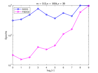
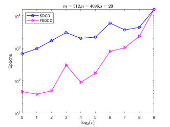
Figure 2. Figures depict the evolution of the number of epochs with respect to the block size $\tau$ for Gaussian matrices. The title of each plot indicates the values of $m,n,s$.

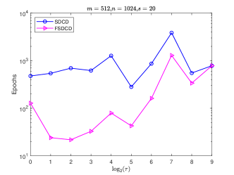
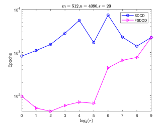
Figure 3. Figures depict the evolution of the number of epochs with respect to the block size $\tau$ for Bernoulli random matrices. The title of each plot indicates the values of $m,n,s$.

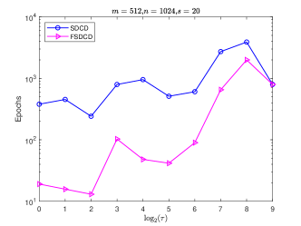
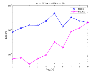
Figure 4. Figures depict the evolution of the number of epochs with respect to the block size $\tau$ for randomly subsampled Hardmard matrices. The title of each plot indicates the values of $m,n,s$.

5.2. Comparison to the existing methods

We compare the performance of the following methods for solving (37): (1) alternating direction method of multipliers (ADMM) [10, 30, 72]; (2) linearized Bregman iteration [13, 12] (denoted by LB); (3) Nesterov accelerated linearized Bregman iteration [34] (denoted by ALB); (4) our proposed methods (SDCD and FSDCD). In particular, we use the following iteration strategy adopted from [72, Remark 1] for the ADMM method

$$x^{k+1} =S_{\nu/\beta}\left(x-\tau A^{\top}(Ax^{k}-b-y^{k}/\beta)\right),$$

$$y^{k+1} =y^{k}-\gamma\beta(Ax^{k+1}-b),$$

where $\beta>0$ is a penalty parameter and $\nu,\gamma>0$ satisfy $\nu\|A\|^{2}_{2}+\gamma<2$. In our test, we set $\nu=\frac{1}{\|A\|_{2}^{2}},\gamma=0.99$, and $\beta=0.01$. The ALB method has the following iteration

$$x^{k+1} =S_{\mu}(\tilde{z}^{k}),$$

$$z^{k+1} =\tilde{z}^{k}-\alpha A^{\top}(Ax^{k+1}-b),$$

$$\tilde{z}^{k+1} =t_{k}z^{k+1}+(1-t_{k})z^{k},$$

where $\alpha=\frac{2}{\|A\|_{2}^{2}}$ and $t_{k-1}=1+\theta_{k}(\theta_{k-1}^{-1}-1)$ with $\theta_{-1}=1$ and $\theta_{k}=\frac{2}{k+2}$ for $k\geq 0$; See [34, Theorem 3.3] for more details. For the ADMM method, we set $x^{0}=0$ and $y^{0}=0$, and for the ALB method, we set $\tilde{z}^{0}=0$.

Figures 5, 6, and 7 illustrate the performance comparisons of ADMM, LB, ALB, SDCD, and FSDCD with different types of sensing matrices. It can be observed from Figures 5 and 6 that when the sensing matrices are Gaussian matrices or Bernoulli random matrices, the SDCD method exhibits faster convergence compared to the LB method. This implies that stochastic algorithms could have advantages over deterministic algorithms at least for some specific types of problems. Furthermore, across all tests presented in the figures, it is evident that the FSDCD method consistently outperforms the other methods. Specially, the FSDCD method is about two times faster than the ALB method, whereas the ALB algorithm is faster than other algorithms.

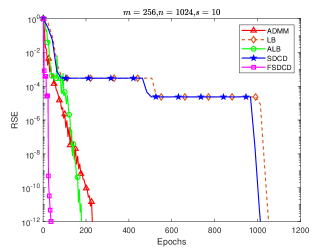
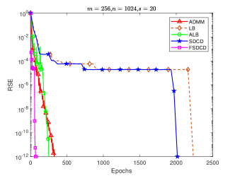
Figure 5. The decrease of RSE across epochs for ADMM, LB, ALB, SDCD, and FSDCD with Gaussian matrices. The title of each plot indicates the values of $m,n,s$.

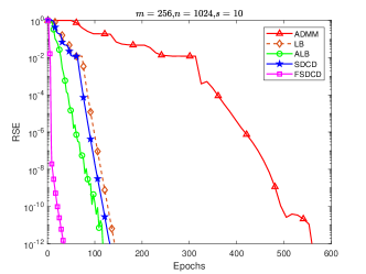
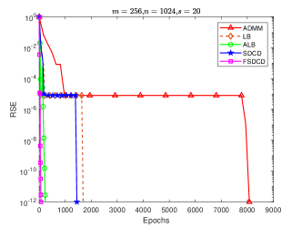
Figure 6. The decrease of RSE across epochs for ADMM, LB, ALB, SDCD, and FSDCD with Bernoulli random matrices. The title of each plot indicates the values of $m,n,s$.

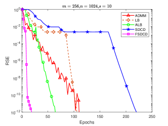
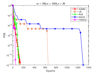
Figure 7. The decrease of RSE across epochs for ADMM, LB, ALB, SDCD, and FSDCD with randomly subsampled Hadamard matrices. The title of each plot indicates the values of $m,n,s$.

6. Concluding remarks

This paper proposed a fast stochastic dual coordinate descent algorithmic framework, FSDCD, for minimizing a strongly convex objective function subject to linear constraints. In particular, we incorporated the heavy ball momentum into our framework and proposed a novel strategy for adaptively learning the parameters $\alpha_{k}$ and $\beta_{k}$ using iteration information. If the objective function $f(x)=\frac{\gamma}{2}\|x-u\|^{2}_{2}-v$, then the deterministic version of our method is serendipitously equivalent to the conjugate gradient normal equation error (CGNE) method. Additionally, we also discussed the extension and the geometric interpretation of our approach. Numerical results confirmed the efficiency of the FSDCD method.

There are still many possible future avenues of research. The linearized Bregman method via split feasibility problems has been investigated in [45], which should be a valuable topic to explore the extensions of the adaptive heavy ball momentum approach for solving the general split feasibility problems. Recently, the Bregman-Kaczmarz method for solving nonlinear systems of equations was studied in [25]. The convenience of extending our methods to nonlinear systems of equations would be a promising avenue for future research. The stochastic heavy ball momentum has been studied in [43], and it is also a valuable topic to investigate the stochastic coordinate descent with adaptive stochastic heavy ball momentum for minimizing the general $L$-smooth convex functions. Furthermore, one can adopt the backtracking rule [7] to learn the parameter $L$.

References

• [1] Z.-Z. Bai and J.-Y. Pan. Matrix analysis and computations. SIAM, 2021.
• [2] Z.-Z. Bai and W.-T. Wu. On greedy randomized Kaczmarz method for solving large sparse linear systems. SIAM J. Sci. Comput., 40(1):A592–A606, 2018.
• [3] Z.-Z. Bai and W.-T. Wu. Randomized Kaczmarz iteration methods: Algorithmic extensions and convergence theory. Japan Journal of Industrial and Applied Mathematics, pages 1–23, 2023.
• [4] M. Barré, A. Taylor, and A. d’Aspremont. Complexity guarantees for Polyak steps with momentum. In Conference on Learning Theory, pages 452–478. PMLR, 2020.
• [5] A. Beck. First-order methods in optimization. SIAM, 2017.
• [6] A. Beck and M. Teboulle. Mirror descent and nonlinear projected subgradient methods for convex optimization. Operations Research Letters, 31(3):167–175, 2003.
• [7] A. Beck and M. Teboulle. A fast iterative shrinkage-thresholding algorithm for linear inverse problems. SIAM journal on imaging sciences, 2(1):183–202, 2009.
• [8] D. P. Bertsekas. Constrained optimization and Lagrange multiplier methods. Academic press, 2014.
• [9] R. Bollapragada, T. Chen, and R. Ward. On the fast convergence of minibatch heavy ball momentum. arXiv preprint arXiv:2206.07553, 2022.
• [10] S. Boyd, N. Parikh, E. Chu, B. Peleato, J. Eckstein, et al. Distributed optimization and statistical learning via the alternating direction method of multipliers. Foundations and Trends® in Machine learning, 3(1):1–122, 2011.
• [11] J.-F. Cai, E. J. Candès, and Z. Shen. A singular value thresholding algorithm for matrix completion. SIAM Journal on optimization, 20(4):1956–1982, 2010.
• [12] J.-F. Cai, S. Osher, and Z. Shen. Convergence of the linearized Bregman iteration for $\ell_{1}$-norm minimization. Mathematics of Computation, 78(268):2127–2136, 2009.
• [13] J.-F. Cai, S. Osher, and Z. Shen. Linearized Bregman iterations for compressed sensing. Mathematics of computation, 78(267):1515–1536, 2009.
• [14] E. J. Candès, J. Romberg, and T. Tao. Robust uncertainty principles: Exact signal reconstruction from highly incomplete frequency information. IEEE Transactions on Information Theory, 52(2):489–509, 2006.
• [15] Y. Censor. Row-action methods for huge and sparse systems and their applications. SIAM review, 23(4):444–466, 1981.
• [16] A. Chambolle and T. Pock. An introduction to continuous optimization for imaging. Acta Numerica, 25:161–319, 2016.
• [17] K.-W. Chang, C.-J. Hsieh, and C.-J. Lin. Coordinate descent method for large-scale l2-loss linear support vector machines. J. Mach. Learn. Res., 9(7):1369—1398, 2008.
• [18] L. Chen, D. Sun, and K.-C. Toh. An efficient inexact symmetric Gauss–Seidel based majorized ADMM for high-dimensional convex composite conic programming. Mathematical Programming, 161:237–270, 2017.
• [19] X. Chen and J. Qin. Regularized Kaczmarz algorithms for tensor recovery. SIAM J. Imaging Sci., 14(4):1439–1471, 2021.
• [20] D. L. Donoho. Compressed sensing. IEEE Transactions on Information Theory, 52(4):1289–1306, 2006.
• [21] R. D’Orazio, N. Loizou, I. Laradji, and I. Mitliagkas. Stochastic mirror descent: Convergence analysis and adaptive variants via the mirror stochastic Polyak stepsize. arXiv preprint arXiv:2110.15412, 2021.
• [22] E. Ghadimi, H. R. Feyzmahdavian, and M. Johansson. Global convergence of the heavy-ball method for convex optimization. In 2015 European control conference (ECC), pages 310–315. IEEE, 2015.
• [23] G. H. Golub and C. F. Van Loan. Matrix computations. JHU press, 2013.
• [24] R. Gordon, R. Bender, and G. T. Herman. Algebraic reconstruction techniques (ART) for three-dimensional electron microscopy and X-ray photography. J. Theor. Biol., 29(3):471–481, 1970.
• [25] R. Gower, D. A. Lorenz, and M. Winkler. A Bregman-Kaczmarz method for nonlinear systems of equations. arXiv preprint arXiv:2303.08549, 2023.
• [26] R. M. Gower, D. Molitor, J. Moorman, and D. Needell. On adaptive sketch-and-project for solving linear systems. SIAM J. Matrix Anal. Appl., 42(2):954–989, 2021.
• [27] R. M. Gower and P. Richtárik. Randomized iterative methods for linear systems. SIAM J. Matrix Anal. Appl., 36(4):1660–1690, 2015.
• [28] M. Griebel and P. Oswald. Greedy and randomized versions of the multiplicative Schwarz method. Linear Algebra Appl., 437(7):1596–1610, 2012.
• [29] D. Han and J. Xie. On pseudoinverse-free randomized methods for linear systems: Unified framework and acceleration. arXiv preprint arXiv:2208.05437, 2022.
• [30] D.-R. Han. A survey on some recent developments of alternating direction method of multipliers. J. Oper. Res. Soc. China, 10(1):1–52, 2022.
• [31] M. Hardt, B. Recht, and Y. Singer. Train faster, generalize better: Stability of stochastic gradient descent. In Proc. 33th Int. Conf. Machine Learning, pages 1225–1234. PMLR, 2016.
• [32] X. He, R. Hu, and Y.-P. Fang. Fast primal–dual algorithm via dynamical system for a linearly constrained convex optimization problem. Automatica, 146:110547, 2022.
• [33] G. T. Herman and L. B. Meyer. Algebraic reconstruction techniques can be made computationally efficient (positron emission tomography application). IEEE Trans. Medical Imaging, 12(3):600–609, 1993.
• [34] B. Huang, S. Ma, and D. Goldfarb. Accelerated linearized Bregman method. Journal of Scientific Computing, 54(2-3):428–453, 2013.
• [35] S. Karczmarz. Angenäherte auflösung von systemen linearer glei-chungen. Bull. Int. Acad. Pol. Sic. Let., Cl. Sci. Math. Nat., pages 355–357, 1937.
• [36] M.-J. Lai and W. Yin. Augmented $\ell_{1}$ and nuclear-norm models with a globally linearly convergent algorithm. SIAM Journal on Imaging Sciences, 6(2):1059–1091, 2013.
• [37] G. Lan. First-order and stochastic optimization methods for machine learning. Springer, 2020.
• [38] G. Lan, A. Nemirovski, and A. Shapiro. Validation analysis of mirror descent stochastic approximation method. Mathematical programming, 134(2):425–458, 2012.
• [39] D. Leventhal and A. S. Lewis. Randomized methods for linear constraints: convergence rates and conditioning. Math. Oper. Res., 35(3):641–654, 2010.
• [40] M. Li, D. Sun, and K.-C. Toh. A majorized ADMM with indefinite proximal terms for linearly constrained convex composite optimization. SIAM Journal on Optimization, 26(2):922–950, 2016.
• [41] Z. Lin, H. Li, and C. Fang. Accelerated optimization for machine learning. Nature Singapore: Springer, 2020.
• [42] J. Liu and S. Wright. An accelerated randomized Kaczmarz algorithm. Math. Comp., 85(297):153–178, 2016.
• [43] N. Loizou and P. Richtárik. Momentum and stochastic momentum for stochastic gradient, newton, proximal point and subspace descent methods. Comput. Optim. Appl., 77(3):653–710, 2020.
• [44] N. Loizou and P. Richtárik. Revisiting randomized gossip algorithms: General framework, convergence rates and novel block and accelerated protocols. IEEE Trans. Inform. Theory, 67(12):8300–8324, 2021.
• [45] D. A. Lorenz, F. Schöpfer, and S. Wenger. The linearized Bregman method via split feasibility problems: analysis and generalizations. SIAM Journal on Imaging Sciences, 7(2):1237–1262, 2014.
• [46] D. A. Lorenz and M. Winkler. Minimal error momentum Bregman-Kaczmarz. arXiv preprint arXiv:2307.15435, 2023.
• [47] H. Luo. Accelerated primal-dual methods for linearly constrained convex optimization problems. arXiv preprint arXiv:2109.12604, 2021.
• [48] H. Luo. A primal-dual flow for affine constrained convex optimization. ESAIM: Control, Optimisation and Calculus of Variations, 28:33, 2022.
• [49] H. Luo and L. Chen. From differential equation solvers to accelerated first-order methods for convex optimization. Mathematical Programming, 195(1-2):735–781, 2022.
• [50] A. Ma and D. Needell. Stochastic gradient descent for linear systems with missing data. Numerical Mathematics: Theory, Methods and Applications, 12(1):1–20, 2019.
• [51] P. Mertikopoulos, B. Lecouat, H. Zenati, C.-S. Foo, V. Chandrasekhar, and G. Piliouras. Optimistic mirror descent in saddle-point problems: Going the extra (gradient) mile. arXiv preprint arXiv:1807.02629, 2018.
• [52] P. Mertikopoulos and M. Staudigl. Stochastic mirror descent dynamics and their convergence in monotone variational inequalities. Journal of optimization theory and applications, 179(3):838–867, 2018.
• [53] J. D. Moorman, T. K. Tu, D. Molitor, and D. Needell. Randomized Kaczmarz with averaging. BIT., 61(1):337–359, 2021.
• [54] M. S. Morshed, S. Ahmad, et al. Stochastic steepest descent methods for linear systems: Greedy sampling & momentum. arXiv preprint arXiv:2012.13087, 2020.
• [55] I. Necoara. Faster randomized block Kaczmarz algorithms. SIAM J. Matrix Anal. Appl., 40(4):1425–1452, 2019.
• [56] I. Necoara. Stochastic block projection algorithms with extrapolation for convex feasibility problems. Optimization Methods and Software, 37(5):1845–1875, 2022.
• [57] D. Needell and J. A. Tropp. Paved with good intentions: analysis of a randomized block Kaczmarz method. Linear Algebra and its Applications, 441:199–221, 2014.
• [58] A. Nemirovski, A. Juditsky, G. Lan, and A. Shapiro. Robust stochastic approximation approach to stochastic programming. SIAM Journal on optimization, 19(4):1574–1609, 2009.
• [59] A. S. Nemirovskij and D. B. Yudin. Problem complexity and method efficiency in optimization. 1983.
• [60] B. T. Polyak. Some methods of speeding up the convergence of iteration methods. Comput. Math. Math. Phys., 4(5):1–17, 1964.
• [61] B. Recht, M. Fazel, and P. A. Parrilo. Guaranteed minimum-rank solutions of linear matrix equations via nuclear norm minimization. SIAM review, 52(3):471–501, 2010.
• [62] P. Richtárik and M. Takácv. Stochastic reformulations of linear systems: Algorithms and convergence theory. SIAM J. Matrix Anal. Appl., 41(2):487–524, 2020.
• [63] H. Robbins and S. Monro. A stochastic approximation method. The Annals of Mathematical Statistics, pages 400–407, 1951.
• [64] R. T. Rockafellar. Convex analysis, volume 11. Princeton university press, 1997.
• [65] F. Schöpfer. Linear convergence of descent methods for the unconstrained minimization of restricted strongly convex functions. SIAM Journal on Optimization, 26(3):1883–1911, 2016.
• [66] F. Schöpfer and D. A. Lorenz. Linear convergence of the randomized sparse Kaczmarz method. Math. Program., 173(1):509–536, 2019.
• [67] O. Sebbouh, R. M. Gower, and A. Defazio. Almost sure convergence rates for stochastic gradient descent and stochastic heavy ball. In Conference on Learning Theory, pages 3935–3971. PMLR, 2021.
• [68] T. Strohmer and R. Vershynin. A randomized Kaczmarz algorithm with exponential convergence. J. Fourier Anal. Appl., 15(2):262–278, 2009.
• [69] L. Tondji and D. A. Lorenz. Faster randomized block sparse Kaczmarz by averaging. Numerical Algorithms, pages 1–35, 2022.
• [70] J. A. Tropp. Column subset selection, matrix factorization, and eigenvalue optimization. In Proceedings of the twentieth annual ACM-SIAM symposium on Discrete algorithms, pages 978–986. SIAM, 2009.
• [71] J.-X. Xie and Z.-Q. Xu. Subset selection for matrices with fixed blocks. Israel J. Math., 245(1):1–26, 2021.
• [72] J. Yang and Y. Zhang. Alternating direction algorithms for $\ell_{1}$-problems in compressive sensing. SIAM Journal on Scientific Computing, 33(1):250–278, 2011.
• [73] W. Yin. Analysis and generalizations of the linearized Bregman method. SIAM Journal on Imaging Sciences, 3(4):856–877, 2010.
• [74] W. Yin, S. Osher, D. Goldfarb, and J. Darbon. Bregman iterative algorithms for $\ell_{1}$ minimization with applications to compressed sensing. SIAM Journal on Imaging sciences, 1(1):143–168, 2008.
• [75] Z. Yun, D. Han, Y. Su, and J. Xie. Fast stochastic dual coordinate descent algorithms for linearly constrained convex optimization. arXiv preprint arXiv:2307.16702, version 1, 2023.
• [76] Y. Zeng, D. Han, Y. Su, and J. Xie. On adaptive stochastic heavy ball momentum for solving linear systems. arXiv preprint arXiv:2305.05482, 2023.
• [77] Y. Zeng, D. Han, Y. Su, and J. Xie. Randomized Kaczmarz method with adaptive stepsizes for inconsistent linear systems. Numerical Algorithms, pages 1–18, 2023.