Electron correlations and superconductivity in La₃Ni₂O₇ under pressure tuning

Abstract

Motivated by the recent discovery of superconductivity in La₃Ni₂O₇ under pressure, we discuss the basic ingredients of a model that captures its microscopic physics under pressure tuning. We anchor our description in terms of the spectroscopic evidence of strong correlations in this system. In a bilayer Hubbard model including the Ni $3d$ $x^{2}-y^{2}$ and $z^{2}$ orbitals, we show the ground state of the model crosses over from a low-spin $S=1/2$ state to a high-spin $S=3/2$ state. In the high-spin state, the two $x^{2}-y^{2}$ and the bonding $z^{2}$ orbitals are all close to half-filling, which promotes a strong orbital selectivity in a broad crossover regime of the phase diagram pertinent to the system. Based on these results, we construct an effective multiorbital $t$-$J$ model to describe the superconductivity of the system, and find the leading pairing channel to be an intraorbital spin singlet with a competition between the extended $s$-wave and $d_{x^{2}-y^{2}}$ symmetries. Our results highlight the role of strong multiorbital correlation effects in driving the superconductivity of La₃Ni₂O₇.

Introduction.  The discovery of iron-based superconductors more than a decade ago provided hope for high temperature superconductivity in a variety of transition-metal-based materials Kamihara_JACS_2008 ; Johnston_2010 ; Si-Hussey_2023 . The recent discovery of superconductivity in a bilayer Ni-based compound La₃Ni₂O₇, with a transition temperature of about $80$ K when the applied pressure exceeds $14$ GPa SunWang_Nature_2023 , was soon confirmed Cheng_arXiv_2023 and zero resistivity was recently obtained Yuan_arXiv_2023 . Unlike the infinite-layer nickelate (Sr,Nd)NiO₂ thin films Li_Nature_2019 , which was expected to resemble the physics of the cuprates given the valence count of Ni¹⁺ with a $d^{9}$ electron configuration, a simple valence count gives Ni^2.5+ in the bilayer compound La₃Ni₂O₇, corresponding to $d^{7.5}$. These results have naturally attracted extensive interest Yao_arXiv_2023 ; Hu_arXiv_2023 ; Werner_arXiv_2023 ; WangQ_arXiv_2023 ; Lechermann_arXiv_2023 ; ZhangG_arXiv_2023 ; Leonov_arXiv_2023 ; Dagotto_arXiv_2023 ; Kuroki_arXiv_2023 ; Zhang_arXiv_2023 ; Lu_arXiv_2023 ; YangF_arXiv_2023 ; Yang_arXiv_2023 ; Wang_arXiv_2023 ; WuYang_arXiv_2023 .

Some of the key questions concern the roles of multiple orbitals and electron correlations Wen_arXiv_2023 for both the normal state and superconductivity of La₃Ni₂O₇. The first-principles density functional theory (DFT) calculation SunWang_Nature_2023 ; SM shows that the bands near the Fermi level have mainly Ni $e_{g}$ orbital characters; bands with $t_{2g}$ orbital characters are located about $2$ eV below the Fermi level. It also reveals a strong inter-layer hopping between the two Ni $z^{2}$ orbitals through the apical oxygen ion, which leads to the formation of bonding-antibonding molecular orbitals (MOs) as illustrated in Fig. 1(a). Considering DFT results and the simple valence count, a naïve picture of the electron state is as follows: Within a two-Ni unit cell, the $t_{2g}$ orbitals are almost fully occupied, and the four $e_{g}$ molecular orbitals are occupied by three electrons. To make progress, it is important to understand the exact ground-state configuration and the low-energy electronic degrees of freedom that underlie the normal state and are responsible for the superconductivity.

In this Letter, we address these important issues by studying the electron correlations in a bilayer two-orbital Hubbard model for La₃Ni₂O₇. Importantly, we anchor our description in terms of the spectroscopically derived experimental evidence for strong correlations Wen_arXiv_2023 . One of our key findings is to show that the electron correlations drive the ground state from a low-spin $S=1/2$ configuration to a high-spin $S=3/2$ one. In the broad crossover regime of the phase diagram, the system exhibits strong orbital selectivity. This regime falls in the parameter range pertinent to La₃Ni₂O₇, as highlighted in Fig. 1(b). We clarify the nature of this crossover regime by showing that further increasing the interaction strength stabilizes an orbital-selective Mott phase (OSMP) in which the two $x^{2}-y^{2}$ orbitals are Mott localized whereas the $z^{2}$ orbitals remain itinerant: Thus, a proximity to the OSMP underlies the strong orbital selectivity seen in the crossover regime. Our results provide the natural understanding of the recent optical conductivity experiments, which provided evidence that the electrons’ kinetic energy is less than $0.1$ of its noninteracting counterpart Wen_arXiv_2023 and that the Drude peak contains two components Wen_arXiv_2023 . Our results on the correlation effect, in turn, allow us to advance the low-energy physics that drives the superconductivity.

Model and method.  We consider a bilayer multiorbital Hubbard model for the two $e_{g}$ orbitals of Ni: $H=H_{\rm{TB}}+H_{\rm{int}}$. Here, $H_{\rm{TB}}$ is a tight-binding Hamiltonian.

$$H_{\rm{TB}} =\frac{1}{2}\sum_{i\delta_{n(z)}\alpha\beta\sigma}t^{\alpha\beta}_{\delta_{n(z)}}d^{\dagger}_{i\alpha\sigma}d_{i+\delta_{n(z)}\beta\sigma}$$ (1)

$$+\sum_{i\alpha\sigma}(\epsilon_{\alpha}-\mu)d^{\dagger}_{i\alpha\sigma}d_{i\alpha\sigma},$$

where $d^{\dagger}_{i\alpha\sigma}$ creates an electron in orbital $\alpha$ ($\alpha=x,z$ denoting the two $e_{g}$ orbitals, $x^{2}-y^{2}$ and $z^{2}$, respectively) with spin $\sigma$ at site $i$ of a bilayer square lattice, $\delta_{n(z)}$ denotes the $n$-th neighboring site in the same (opposite) layer, $\epsilon_{\alpha}$ refers to the energy level associated with the crystal field splittings, and $\mu$ is the chemical potential. The tight-binding parameters $t^{\alpha\beta}_{\delta_{n(z)}}$ and $\epsilon_{\alpha}$ are obtained by fitting the calculated DFT band structure and projecting to the two-$e_{g}$-orbital basis in a unit cell including two Ni sites as described in the Supplemental Material (SM) SM . We adjust the chemical potential so that the total electron density is $3$ per unit cell to reflect the valence count of Ni^2.5+. The on-site interaction $H_{\rm{int}}$ reads

$$H_{\rm{int}} = \frac{U}{2}\sum_{i,\alpha,\sigma}n_{i\alpha\sigma}n_{i\alpha\bar{\sigma}}$$ (2)

$$+ \sum_{i,\alpha<\beta,\sigma}\left\{U^{\prime}n_{i\alpha\sigma}n_{i\beta\bar{\sigma}}\right.+(U^{\prime}-J_{\rm{H}})n_{i\alpha\sigma}n_{i\beta\sigma}$$

$$- \left.J_{\rm{H}}(d^{\dagger}_{i\alpha\sigma}d_{i\alpha\bar{\sigma}}d^{\dagger}_{i\beta\bar{\sigma}}d_{i\beta\sigma}+d^{\dagger}_{i\alpha\sigma}d^{\dagger}_{i\alpha\bar{\sigma}}d_{i\beta\sigma}d_{i\beta\bar{\sigma}})\right\},~{}$$

where $n_{i\alpha\sigma}=d^{\dagger}_{i\alpha\sigma}d_{i\alpha\sigma}$. Here, $U$, $U^{\prime}$, and $J_{\rm{H}}$, respectively denote the intra- and inter- orbital repulsion and the Hund’s rule coupling, and $U^{\prime}=U-2J_{\rm{H}}$ is taken Castellani_PRB_1978 .

As already mentioned, the strong hopping between the two Ni $z^{2}$ orbitals in the upper and lower layers causes bonding-antibonding MO states. To examine this bonding effect, we perform a transformation from the atomic orbital basis to the bonding MO basis, namely by defining the MO as

$$d_{i\alpha\sigma}^{b(a)}=\frac{1}{\sqrt{2}}(d_{i\alpha\sigma}\pm d_{i+\delta_{0z}\alpha\sigma}),$$ (3)

where the index $b(a)$ corresponds to the bonding (antibonding) MO, and $i$ ($i+\delta_{0z}$) on the right hand side refers to a site in the top (bottom) layer. Note that we define MOs for both $z^{2}$ and $x^{2}-y^{2}$ orbitals for convenience, though the $x^{2}-y^{2}$ orbital is expected to be largely non-bonding given the small inter-layer hopping amplitude associated with this orbital SM . We can rewrite the tight-binding and interaction Hamiltonians of Eqns. (1) and (2) in the MO basis. In particular,

$$H_{\rm{int}} = H_{\rm{int}}^{b-b}+H_{\rm{int}}^{b-a},$$ (4)

where $H_{\rm{int}}^{b-b}$ refers to the interactions between bonding (or antibonding) states, whereas $H_{\rm{int}}^{b-a}$ refers to the interactions mixing the bonding and antibonding states. The exact forms of $H_{\rm{int}}^{b-b}$ and $H_{\rm{int}}^{b-a}$ are presented in the SM SM .

The correlation effects of the above model in the MO basis are then investigated by using a $U(1)$ slave-spin theory Yu_PRB_2012 ; Yu_PRB_2017 . In this approach, the $d$-electron operators are rewritten as $d^{\dagger}_{i\alpha\sigma}=S^{+}_{i\alpha\sigma}f^{\dagger}_{i\alpha\sigma}$ (here we absorb the MO index in $\alpha$), where $S^{+}_{i\alpha\sigma}$ ($f^{\dagger}_{i\alpha\sigma}$) is a quantum $S=1/2$ spin (fermionic spinon) operator introduced to carry the electron’s charge (spin) degree of freedom, and $S^{z}_{i\alpha\sigma}=f^{\dagger}_{i\alpha\sigma}f_{i\alpha\sigma}-\frac{1}{2}$ is a local constraint. At the saddle-point level, we employ a Lagrange multiplier $\lambda_{\alpha}$ to handle the constraint, and decompose the slave-spin and spinon operators. In this way, the model rewritten in the slave-spin representation is solved by determining $\lambda_{\alpha}$ and the quasiparticle spectral weight $Z_{\alpha}\propto|\langle S^{+}_{\alpha}\rangle|^{2}$ self-consistently Yu_PRB_2012 ; Yu_PRB_2017 .

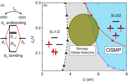
Figure 1: (Color online) (a): Sketch of formation of the bonding-antibonding MO states between the Ni $z^{2}$ orbitals in the top and bottom layers. (b): Ground-state phase diagram in the $U$-$J_{\rm{H}}$ plane of the bilayer two-orbital Hubbard model for La₃Ni₂O₇, calculated by the $U(1)$ slave-spin theory in the MO basis. Red line with squares shows the transition between the low-spin $S=1/2$ state to the high-spin $S=3/2$ state in the atomic limit. Blue regime is the orbital-selective Mott phase (OSMP) in which the $x^{2}-y^{2}$ orbitals are Mott localized whereas the $z^{2}$ orbitals are itinerant (see Fig. 2(a)). The dahsed line with triangles characterizes the low-spin to high-spin crossover, and in the gray regime the system exhibits strong orbital selectivity (see text). Highlighted by the golden shading in the plot is the parameter region pertinent to La₃Ni₂O₇.

Low-spin to high-spin crossover and orbital-selective Mott physics.  We first diagonalize the interaction Hamiltonian of Eqn. (4) in the MO basis. The ground state is either a low-spin $S=1/2$ state at small $J_{\rm{H}}$ or a high-spin $S=3/2$ state at large $J_{\rm{H}}$ SM . In the low-spin state, the $z^{2}$ bonding state is largely doubly occupied, whereas the antibonding state is almost empty. The $x^{2}-y^{2}$ orbitals are near quarter filling. In the high-spin state, on the other hand, the bonding $z^{2}$ and $x^{2}-y^{2}$ orbitals are all half filled, and the antibonding $z^{2}$ state keeps empty. Either the low-spin or the high-spin configuration is four-fold degenerate. For the low-spin state, the additional degeneracy comes from the doubly degenerate $x^{2}-y^{2}$ orbitals, which can be described by an isospin $\tau=1/2$. The transition from the low-spin to high-spin state is shown as the red line with square symbols in Fig. 1(b). In the presence of electron hopping, this transition turns to a crossover.

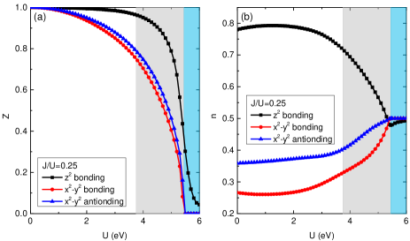
Figure 2: (Color online) Evolution of the orbital-resolved quasiparticle spectral weight $Z$ [in (a)] and electron density $n$ [in (b)] with increasing $U$ at $J_{\rm{H}}/U=0.25$ of the bilayer two-orbital model in the MO basis calculated by using the $U(1)$ slave-spin theory. The blue and gray regimes correspond to OSMP and metallic state with strong orbital selectivity, respectively.

To examine how this crossover takes place in the multiorbital Hubbard model, we perform slave-spin calculation in the MO basis. Note that the antibonding $z^{2}$ state has a very low electron density $n<0.1$ at $U=0$. Accordingly, we expect it to be only weakly affected by interactions. To simplify the calculation, we set $Z=1$ in this MO and turn off interaction terms associated with this orbital. The results of the slave-spin calculation is summarized in the phase diagram of Fig. 1(b). The dashed line characterizes the low-spin to high-spin crossover SM . Across this crossover line with increasing $U$ to the gray regime, the system exhibits strong orbital selectivity: As shown in Fig. 2(a), quasiparticle spectral weights and electron densities in all orbitals change drastically and $Z_{x^{2}-y^{2}}\ll Z_{z^{2}}$ in this regime. Further increasing $U$, the system undergoes an orbital-selective Mott transition (OSMT) to an OSMP at the blue line with circles. As shown in Fig. 2, in the OSMP $Z_{x^{2}-y^{2}}=0$ and $n_{x^{2}-y^{2}}=1/2$, but $Z_{z^{2}(b)}>0$: The electrons in the $x^{2}-y^{2}$ orbitals are Mott localized whereas those in the $z^{2}$ bonding states are still itinerant, though very close to the Mott localization.

The OSMP is associated with the high-spin state. One sees from Fig. 2(b) that in this state the electron densities of the $x^{2}-y^{2}$ and $z^{2}$ bonding orbitals are all close to $1/2$. If the antibonding state were to be completely empty, the system consisting of the other three orbitals would be exactly at half-filling and becomes Mott insulating when the red line of transition is approached. However, at finite $U$ an OSMP is more favorable because keeping the $z^{2}$ bonding orbital itinerant reduces the kinetic energy. This naturally explains why the OSMT line almost traces the red transition line to the high-spin Mott insulator (MI), especially when $J_{\rm{H}}/U$ is large.

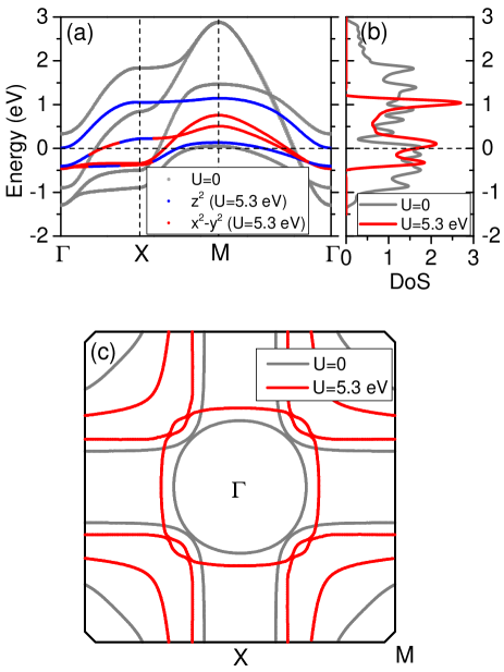
Figure 3: (Color online) (a): Bandstructure at $U=5.3$ eV compared to the one at $U=0$, indicating strong orbital-selective band renormalization. (b): The corresponding electron density of states (DoS) showing a large renormalization on the bandwidth $W$. (c): Comparison of the Fermi surface at $U=5.3$ eV and $U=0$.

We next consider the effects of orbital-selective Mott correlations to the electronic structure. Fig. 3(a) shows the bands along high-symmetry directions of the Brillouin zone at $U=5.3$ eV compared to those at $U=0$. Close to the OSMP, bands with the $x^{2}-y^{2}$ and $z^{2}$ bonding orbital characters are strongly renormalized whereas the $z^{2}$ antibonding band, located topmost in energy, only hardly shifts compared to the $U=0$ case. As shown in Fig. 3(b) and (c), compared to the significant renormalization in the total bandwidth $W$ from about $4$ eV to about $1.5$ eV, the Fermi surface only changes moderately. While the relatively small inner hole pocket centered at the M point exhibits a sizable expansion, the outer hole and electron pockets centered around the $\Gamma$ point only slightly shrink and expand, respectively.

Figure 4: (Color online) Evolution of the leading superconducting pairing symmetry, from an extended $s$-wave $A^{1g}$ to a $d$-wave $B^{1g}$ with increasing $J^{xx}$. Here we take $J^{zz}=0.025W_{0}$, and vary the ratio $r=J^{xx}/J^{zz}$, where $W_{0}$ is the total bandwidth of the multiorbital Hubbard model at $U=0$.

An effective multiorbital $t$-$J$ model for superconductivity.  The above slave-spin results set the stage to build a low-energy effective model in understanding superconductivity of the system, which can be done by performing a $t/U$ perturbation expansion when $U$ is sizeable. However, the resulting form of the effective theory depends on the low-energy manifold the perturbed Hamiltonian is projected to. For example, when projecting to the $S=1/2$ low-spin sector, one ends up with an effective model that includes interactions between the total spin and isospin operators, which takes the form of the Kugel-Khomskii model KK . On the other hand, one obtains three-orbital Heisenberg couplings for the interacting part of the Hamiltonian when projecting to the high-spin sector. Which model is pertinent to the low-energy physics depends on the strength of the interaction.

For La₃Ni₂O₇, $U$ is estimated to be within $4$ to $6$ eV SunWang_Nature_2023 ; Werner_arXiv_2023 . According to the phase diagram in Fig. 1(b), this suggests that the system is in the regime with strong orbital selectivity near the OSMP (as highlighted in Fig. 1(b)). Therefore, we construct the effective model by starting from the $S=3/2$ high-spin ground state, and taking into account effects of the $S=1/2$ low-lying excitations by projecting out doubly occupied states. As a result, it takes the form of a multiorbital $t$-$J$ model where the Hamiltonian reads

$$H_{\rm{eff}} =\frac{1}{2}\sum_{{ij}\alpha\beta\sigma}\sqrt{Z_{\alpha}Z_{\beta}}t^{\alpha\beta}_{ij}f^{\dagger}_{i\alpha\sigma}f_{j\beta\sigma}+\sum_{i\alpha\sigma}(\epsilon^{\prime}_{\alpha}-\mu)f^{\dagger}_{i\alpha\sigma}f_{i\alpha\sigma}$$ (5)

$$+{\sum_{ij\alpha\beta}}^{\prime}J^{\alpha\beta}_{ij}\mathbf{S}_{i\alpha}\cdot\mathbf{S}_{j\beta}.$$

Here we have employed the slave-spin method to renormalize the kinetic part of the Hamiltonian: $Z_{\alpha}$ is the quasiparticle spectral weight of the $\alpha$-th MO, and $\epsilon^{\prime}_{\alpha}$ refers to the renormalized energy level of orbital $\alpha$. This is a generalization of the slave-boson theory Lee_RMP_2006 to the finite $U$ case. $\mathbf{S}_{i\alpha}=\frac{1}{2}f^{\dagger}_{i\alpha s}\boldsymbol{\sigma}_{ss^{\prime}}f_{i\alpha s^{\prime}}$ denotes the spin density operator at site $i$ in the $\alpha$ orbital. Considering the high-spin state, the summation ${\sum}^{\prime}$ runs over the two $x^{2}-y^{2}$ and the one $z^{2}$ bonding MOs. $J^{\alpha\beta}_{ij}$ refers to the orbital dependent exchange coupling which can be determined from the second-order $t/U$ perturbation expansion SM . Here we neglect the inter-layer couplings between $x^{2}-y^{2}$ orbitals and second-nearest and further neighboring interactions because of their small hopping amplitudes, and only consider the in-plane nearest neighboring exchange interactions $J^{xx}_{1}$, $J^{zz}_{1}$, and $J^{xz}_{1}$. We find $J^{xz}_{1}$ to be negligibly small, and $J^{xx}_{1}$, $J^{zz}_{1}$ are antiferromagnetic. In the following, we take the convention $J^{\alpha\beta}$ for $J^{\alpha\beta}_{1}$. To explore how the superconducting pairing evolves with orbital-selective correlations, we take $J^{zz}=0.025W_{0}$ (with $W_{0}$ referring to the bandwidth at $U=0$), and tune the ratio $r=J^{xx}/J^{zz}$.

Superconducting pairing symmetry.  The superconducting pairing in the model of Eqn. (5) is studied by a Bogoliubov mean-field decomposition of the exchange interactions in the intra-orbital spin singlet sector:

$$J^{\alpha\alpha}_{\delta}(\mathbf{S}_{i\alpha}\cdot\mathbf{S}_{i+\delta\alpha}-\frac{1}{4}n_{i\alpha}n_{i+\delta\alpha})~{}~{}~{}~{}~{}~{}~{}~{}~{}~{}$$

$$\approx-\frac{J^{\alpha\alpha}_{\delta}}{2}(\hat{\Delta}^{\dagger}_{\delta\alpha}\Delta_{\delta\alpha}+\rm{h.c.}-|\Delta_{\delta\alpha}|^{2}),$$ (6)

where $\hat{\Delta}_{\delta\alpha}=f_{i\alpha\downarrow}f_{i+\delta\alpha\uparrow}-f_{i\alpha\uparrow}f_{i+\delta\alpha\downarrow}$, and the gap function $\Delta_{\delta\alpha}=\langle\hat{\Delta}_{\delta\alpha}\rangle$. La₃Ni₂O₇ under pressure has an orthorhomic structure. But the difference between the $a$ and $b$ lattice constants is small (about $1\%$) SunWang_Nature_2023 . As such, for convenience, we examine the symmetry of the gap functions by studying how they transform under the tetragonal $D_{4h}$ group. The result is summarized in the SM (Tab. S2) SM . One sees that the multiorbital nature leads to six different pairing channels. We then perform a self-consistent calculation to determine the leading pairing channel Yu_NC_2013 . As shown in Fig. 4, the leading pairing channel changes from the extended $s$-wave $A^{1g}_{z^{2}}$ to $d$-wave $B^{1g}$ in both $x^{2}-y^{2}$ and $z^{2}$-bonding orbitals with increasing $J^{xx}$. In the $A^{1g}$ dominant regime, the pairing is also strongly orbital-selective, with the leading channel associated with the $z^{2}$ bonding orbital. Besides the larger pairing amplitude stabilized by $J^{zz}$, this pairing channel is also favored by causing a full superconducting gap along the inner hole pocket centered at the M point. However, nodes along the outer hole pocket cannot be avoided by either pairing channel. To avoid nodes, it is possible that a pairing function with mixed $s$- and $d$-wave characters, such as the time-reversal breaking $s$+i$d$ Yu_NC_2013 or $s$+$d$ (given the orthorhmic lattice symmetry of the compound) Hu_PRB_2018 , is stabilized in the regime where $A^{1g}$ and $B^{1g}$ pairing channels are in competition.

Discussions and conclusions.  Several remarks are in order. First, as shown in Fig. 2(a), near and inside the OSMP the $z^{2}$ bonding state is also very close to Mott localization. This makes the system to be in proximity to a multiorbital MI, which naturally explains the substantially suppressed Drude weight as observed in a recent optical conductivity measurement Wen_arXiv_2023 . The strong orbital selectivity between the $z^{2}$ and $x^{2}-y^{2}$ orbitals accounts for the observed two-component contribution to the Drude weight Wen_arXiv_2023 . Second, applying a pressure corresponding to increasing the hopping amplitudes, or equivalently, reducing the $U/t$ ratio in our model. This increases the itinerancy of electrons, and causes bandwidth tuning of the superconductivity. But in multiorbital systems, the effects of reducing the $U/t$ ratio has additional effects. It can trigger a high-spin to low-spin crossover, as shown in the present work. This activates the orbital degree of freedom, which makes the exchange couplings orbital dependent and may lead to strong competition of fluctuations in the antiferromagnetic spin and orbital channels as reflected in the complicated temperature evolution of the magnetic susceptibility in La₃Ni₂O₇ at ambient pressure Wu_PRB_2001 ; Liu_SC_2022 . Moreover, reducing the $U/t$ ratio also causes redistribution of the electrons among the orbitals, leading to an effect similar to either hole or electron doping a MI in each orbital. This effect resembles a multiorbital version of the physics in doping the cuprates, which is known to favor superconductivity.

In conclusion, we have studied electron correlation effects in a bilayer two-orbital Hubbard model for La₃Ni₂O₇ in the MO basis, and found a strong orbital selectivity when the interaction strength is moderate. Further increasing the interaction, an OSMP is stabilized. The OSMP is close to an $S=3/2$ high-spin state, in which the $x^{2}-y^{2}$ and $z^{2}$ bonding orbitals are all very close to half-filling. In light of these results, we obtain an effective multiorbital $t$-$J$ model for superconductivity of the system in the crossover regime towards the high-spin configuration. We show that the system exhibits orbital-selective pairing and the leading superconducting pairing channel evolves from the extended $s$-wave $A^{1g}$ to $d$-wave $B^{1g}$ when the intra-orbital nearest-neighbor exchange coupling $J^{xx}$ is increased. Our work paves the way for systematically describing the pressure-induced high-$T_{c}$ superconductivity of La₃Ni₂O₇.

SUPPLEMENTAL MATERIAL – Electron correlations and superconductivity in La₃Ni₂O₇ under pressure tuning

.1 Details on the tight-binding model

To include the realistic band structure at low energies into our tight-binding modeling, we have first carried out band structure calculations for La₃Ni₂O₇ within the framework of density functional theory (DFT). We have used the plane wave basis set as implemented in the Vienna Ab initio Simulation Package (VASP) code vasp_website . Projector augmented-wave potentials and Perdew-Burke-Ernzerhof exchange-correlation functional were used in the calculations. We consider the experimental lattice parameters ($a=5.289\;$Å, $b=5.218\;$Å, $c=19.734\;$Å) SunWang_Nature_2023 in the simulations. Since the difference between $a$ and $b$ is only about 1.3$\%$, we use their average value ($a=b=5.2535\;$Å) in the calculations. Though this procedure has modified the space group from $Fmmm$ to $I4/mmm$, it should have little effect on the electronic structure.

As shown in Fig. S1, the bands near the Fermi energy have mainly the Ni $3d$ $e_{g}$ orbital character. The bands associated with the $t_{2g}$ orbitals are at least $1$ eV below the Fermi level. The oxygen $2p$ bands are dominant at about $4$ eV below the Fermi energy. Therefore, the relevant orbitals within a $2$ eV energy window about the Fermi energy are the Ni $e_{g}$ ones. We hence fit the Wannierized bands with a bilayer $2$-orbital tight-banding Hamiltonian including these $e_{g}$ orbitals in the Brillouin zone (BZ) corresponding to the two Ni (in the top and bottom layers) unit cell. At this step we have used projected Wannier functions; the procedure of disentanglement was performed with the maximally-localized Wannier functions scheme as implemented in the Wannier90 code Pizzi_JPCM_2020 . The tight-binding parameters from the fitting are summarized in Tab. S1.

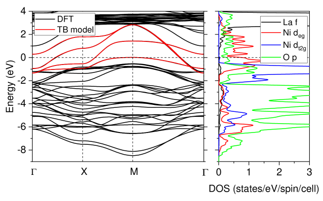
Figure S1: (Color online) (a): Band structure of La₃Ni₂O₇ along high-symmetry directions of the BZ calculated from DFT (black lines) and from the bilayer two-orbital tight-binding model (red lines). (b): The corresponding projected density of states (DOS) calculated from DFT.

The band structure of the bilayer 2-orbital tight-binding model compared to the DFT results is shown in Fig. S1. The tight-binding model reproduces a similar band structure of DFT in the energy window of interest, from $-1.5$ eV to $2.5$ eV.

orbital	$\epsilon$	$t_{1}$	$t_{2}$	$t_{3}$	$t_{0z}$	$t_{1z}$
$xx$	$10.8735$	$-0.4899$	$0.0670$	$-0.0600$	$0.0022$	$0.0003$
$zz$	$10.5142$	$-0.1159$	$-0.0109$	$-0.0187$	$-0.6363$	$0.0231$
$xz$		$\mp 0.2420$	$0$	$\mp 0.0333$	$0$	$\pm 0.0382$

Table S1: Tight-binding parameters of the bilyaer two-orbital model for La₃Ni₂O₇. $xx$ ($zz$) denotes the intra-orbital hopping between the $x^{2}-y^{2}$ ($z^{2}$) orbitals, whereas $xz$ denotes the inter-orbital hopping between the $x^{2}-y^{2}$ and $z^{2}$ orbitals. $t_{n(z)}$ refers to intra- (inter-)layer hopping between the $n$-th neighboring sites. Finally, $\pm$ means that the hopping parameter is positive along the $x$ direction but negative along the $y$ direction. All units are in eV.

.2 The interaction Hamiltonian in the bonding molecular orbital basis and the low-spin to high-spin crossover

In the main text, we have performed a transformation from the atomic orbital basis to the molecular orbital (MO) basis,

$$d_{i\alpha\sigma}^{b(a)}=\frac{1}{\sqrt{2}}(d_{i\alpha\sigma}\pm d_{i+\delta_{0z}\alpha\sigma}),$$ (7)

where the index $b(a)$ corresponds to the bonding (antibonding) MO, and $i$ ($i+\delta_{0z}$) on the right hand side refers to a site in the top (bottom) layer. Here we define MOs for both the $z^{2}$ and $x^{2}-y^{2}$ orbitals for convenience. But as listed in Tab. S1, the inter-layer hopping amplitude between the $x^{2}-y^{2}$ orbitals is much smaller than both its intra-layer counterpart and the inter-layer hopping between the $z^{2}$ orbitals. We therefore expect that the $x^{2}-y^{2}$ orbital is largely non-bonding.

In this MO basis, the interaction Hamiltonian is rewritten to

$$H_{\rm{int}}=H^{b-b}_{\rm{int}}+H^{b-a}_{\rm{int}},$$ (8)

where the boning-bonding and antibonding-antibonding interactions are

$$H^{b-b}_{int} = \frac{U}{2}\sum_{\alpha}(n_{I\alpha\uparrow}^{a}n_{I\alpha\downarrow}^{a}+n_{I\alpha\uparrow}^{b}n_{I\alpha\downarrow}^{b})+\frac{U^{\prime}}{4}\sum_{\alpha\neq\beta,\sigma\neq\sigma^{\prime}}(n_{I\alpha\sigma}^{a}n_{I\beta\sigma^{\prime}}^{a}+n_{I\alpha\sigma}^{b}n_{I\beta\sigma^{\prime}}^{b})$$ (9)

$$+ \frac{U^{\prime}-J}{2}\sum_{\alpha>\beta,\sigma}(n_{I\alpha\sigma}^{a}n_{I\beta\sigma}^{a}+n_{I\alpha\sigma}^{b}n_{I\beta\sigma}^{b})-\frac{J}{2}\sum_{\alpha\neq\beta}(d_{I\alpha\uparrow}^{a+}d_{I\beta\downarrow}^{a+}d_{I\beta\uparrow}^{a}d_{I\alpha\downarrow}^{a}+d_{I\alpha\uparrow}^{b+}d_{I\beta\downarrow}^{b+}d_{I\beta\uparrow}^{b}d_{I\alpha\downarrow}^{b})$$

$$- \frac{J}{2}\sum_{\alpha\neq\beta}(d_{I\alpha\uparrow}^{b+}d_{I\alpha\downarrow}^{b+}d_{I\beta\uparrow}^{b}d_{I\beta\downarrow}^{b}+d_{I\alpha\uparrow}^{a+}d_{I\alpha\downarrow}^{a+}d_{I\beta\uparrow}^{a}d_{I\beta\downarrow}^{a}),$$

and the bonding-antibonding mixing interaction is

$$H^{b-a}_{int} = \frac{U}{2}\sum_{\alpha}(n_{I\alpha\uparrow}^{a}n_{I\alpha\downarrow}^{b}+n_{I\alpha\uparrow}^{b}n_{I\alpha\downarrow}^{a})+\frac{U^{\prime}}{4}\sum_{\alpha\neq\beta,\sigma\neq\sigma^{\prime}}(n_{I\alpha\sigma}^{a}n_{I\beta\sigma^{\prime}}^{b}+n_{I\alpha\sigma}^{b}n_{I\beta\sigma^{\prime}}^{a})+\frac{U^{\prime}-J}{2}\sum_{\alpha>\beta,\sigma}(n_{I\alpha\sigma}^{a}n_{I\beta\sigma}^{b}+n_{I\alpha\sigma}^{b}n_{I\beta\sigma}^{a})$$ (10)

$$+ \frac{U}{2}\sum_{\alpha}(d_{I\alpha\uparrow}^{b+}d_{I\alpha\uparrow}^{a}d_{I\alpha\downarrow}^{b+}d_{I\alpha\downarrow}^{a}+d_{I\alpha\uparrow}^{b+}d_{I\alpha\uparrow}^{a}d_{I\alpha\downarrow}^{a+}d_{I\alpha\downarrow}^{b}+d_{I\alpha\uparrow}^{a+}d_{I\alpha\uparrow}^{b}d_{I\alpha\downarrow}^{b+}d_{I\alpha\downarrow}^{a}+d_{I\alpha\uparrow}^{a+}d_{I\alpha\uparrow}^{b}d_{I\alpha\downarrow}^{a+}d_{I\alpha\downarrow}^{b})$$

$$+ \frac{U^{\prime}}{4}\sum_{\alpha\neq\beta,\sigma\neq\sigma^{\prime}}(d_{I\alpha\sigma}^{b+}d_{I\alpha\sigma}^{a}d_{I\beta\sigma^{\prime}}^{b+}d_{I\beta\sigma^{\prime}}^{a}+d_{I\alpha\sigma}^{b+}d_{I\alpha\sigma}^{a}d_{I\beta\sigma^{\prime}}^{a+}d_{I\beta\sigma^{\prime}}^{b}+d_{I\alpha\sigma}^{a+}d_{I\alpha\sigma}^{b}d_{I\beta\sigma^{\prime}}^{b+}d_{I\beta\sigma^{\prime}}^{a}+d_{I\alpha\sigma}^{a+}d_{I\alpha\sigma}^{b}d_{I\beta\sigma^{\prime}}^{a+}d_{I\beta\sigma^{\prime}}^{b})$$

$$+ \frac{U^{\prime}-J}{2}\sum_{\alpha>\beta,\sigma}(d_{I\alpha\sigma}^{b+}d_{I\alpha\sigma}^{a}d_{I\beta\sigma}^{b+}d_{I\beta\sigma}^{a}+d_{I\alpha\sigma}^{b+}d_{I\alpha\sigma}^{a}d_{I\beta\sigma}^{a+}d_{I\beta\sigma}^{b}+d_{I\alpha\sigma}^{a+}d_{I\alpha\sigma}^{b}d_{I\beta\sigma}^{b+}d_{I\beta\sigma}^{a}+d_{I\alpha\sigma}^{a+}d_{I\alpha\sigma}^{b}d_{I\beta\sigma}^{a+}d_{I\beta\sigma}^{b})$$

$$- \frac{J}{2}\sum_{\alpha\neq\beta}(d_{I\alpha\uparrow}^{a+}d_{I\beta\downarrow}^{a+}d_{I\beta\uparrow}^{b}d_{I\alpha\downarrow}^{b}+d_{I\alpha\uparrow}^{b+}d_{I\beta\downarrow}^{b+}d_{I\beta\uparrow}^{a}d_{I\alpha\downarrow}^{a}+d_{I\alpha\uparrow}^{b+}d_{I\beta\downarrow}^{a+}d_{I\beta\uparrow}^{b}d_{I\alpha\downarrow}^{a}$$

$$+ d_{I\alpha\uparrow}^{b+}d_{I\beta\downarrow}^{a+}d_{I\beta\uparrow}^{a}d_{I\alpha\downarrow}^{b}+d_{I\alpha\uparrow}^{a+}d_{I\beta\downarrow}^{b+}d_{I\beta\uparrow}^{a}d_{I\alpha\downarrow}^{b}+d_{I\alpha\uparrow}^{a+}d_{I\beta\downarrow}^{b+}d_{I\beta\uparrow}^{b}d_{I\alpha\downarrow}^{a})$$

$$- \frac{J}{2}\sum_{\alpha\neq\beta}(d_{I\alpha\uparrow}^{a+}d_{I\alpha\downarrow}^{a+}d_{I\beta\uparrow}^{b}d_{I\beta\downarrow}^{b}+d_{I\alpha\uparrow}^{b+}d_{I\alpha\downarrow}^{b+}d_{I\beta\uparrow}^{a}d_{I\beta\downarrow}^{a}+d_{I\alpha\uparrow}^{b+}d_{I\alpha\downarrow}^{a+}d_{I\beta\uparrow}^{b}d_{I\beta\downarrow}^{a}$$

$$+ d_{I\alpha\uparrow}^{b+}d_{I\alpha\downarrow}^{a+}d_{I\beta\uparrow}^{a}d_{I\beta\downarrow}^{b}+d_{I\alpha\uparrow}^{a+}d_{I\alpha\downarrow}^{b+}d_{I\beta\uparrow}^{a}d_{I\beta\downarrow}^{b}+d_{I\alpha\uparrow}^{a+}d_{I\alpha\downarrow}^{b+}d_{I\beta\uparrow}^{b}d_{I\beta\downarrow}^{a}).$$

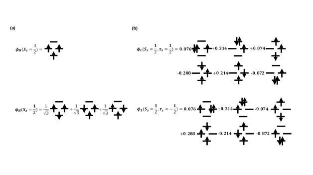
Figure S2: (Color online) (a): High-spin $S=3/2$ ground-state configurations. (b): Low-spin $S=1/2$ ground-state configurations. Each ground state is four-fold degenerate, and the other degenerate configurations can be obtained by reversing the spin direction ($S^{z}\rightarrow-S^{z}$) from those presented here.

Diagonalizing the interaction Hamiltonian along with the onsite potential term in the tight-binding Hamiltonian written in the MO basis, we obtain two ground states in the atomic limit: an $S=1/2$ low-spin state and an $S=3/2$ high-spin state. These two ground states are illustrated in Fig. S2. Each state is four-fold degenerate. In the $S=1/2$ low-spin state, the additional degeneracy is associated with the two degenerate $x^{2}-y^{2}$ orbitals. As one sees, the low-spin configuration is dominated by the Fock state that the bonding $z^{2}$ orbital is doubly occupied while the $x^{2}-y^{2}$ orbitals are quarter filled. We can then define an orbital isospin operator $\boldsymbol{\tau}$, with the Ising variable $\tau^{z}$ denoting the electron density difference in the $x^{2}-y^{2}$ orbitals between the top and bottom layers. The four degenerate low-spin configurations can be obtained from the one shown in Fig. S2 by appying total spin and orbital isospin reversal symmetry, respectively. On the other hand, the degenerate high-spin configurations can be labeled by the quantum number $S^{z}$ of the total spin.

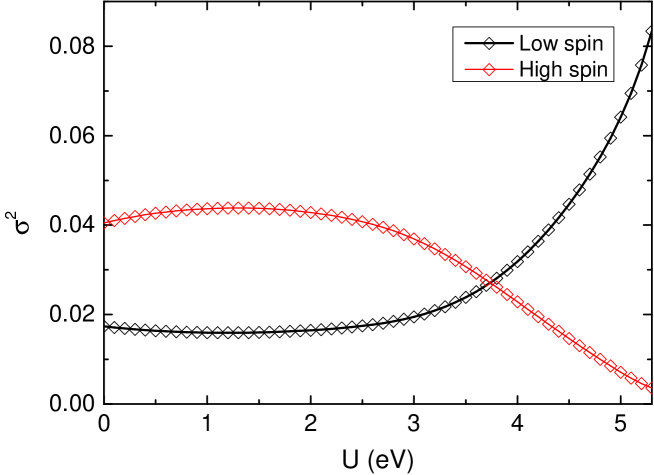
Figure S3: (Color online) Variance of the electron density profile from the low-spin and high-spin states at $J_{\rm{H}}/U=0.25$. The low-spin to high-spin crossover is determined from the crossing point of the two variance curves.

In the atomic limit, there is a transition from the low-spin to high-spin ground state by increasing $J_{\rm{H}}$, shown as the red line in the phase diagram of Fig. 1(b) in the main text. Taking into account the kinetic energy will turn the transition to a crossover. To determine the crossover line in the phase diagram, we define the variances of the electron density profile from that dominating the low- and high-spin states:

$$\sigma^{2}_{L} =\frac{1}{4}\left[(n_{z^{2}(b)}-1)^{2}+(n_{z^{2}(a)})^{2}+2(n_{x^{2}-y^{2}}-1/4)^{2})\right],$$ (11)

$$\sigma^{2}_{H} =\frac{1}{4}\left[(n_{z^{2}(b)}-1/2)^{2}+(n_{z^{2}(a)})^{2}+2(n_{x^{2}-y^{2}}-1/2)^{2})\right].$$ (12)

The variances with $U$ at $J_{\rm{H}}/U=0.25$ is depicted in Fig. S3. The low-spin to high-spin crossover is then determined by the criterion $\sigma^{2}_{H}=\sigma^{2}_{L}$, which gives the dashed line in the phase diagram of Fig. 1(b) in the main text.

.3 Details on the derivation of the effective model

To construct the effective model, we start from the bilayer two-orbital Hubbard model in the MO basis, and rewrite the toal Hamiltonian into two parts, $H=H_{0}+H_{1}$. We take the Hamiltonian in the atomic limit (including the interaction and onsite potential terms) as the unperturbed Hamiltonian $H_{0}$, and treat the hopping terms as perturbations ($H_{1}$). The effective low-energy model can be obtained via a canonical transformation,

$$H_{\rm{eff}}=e^{i\mathcal{S}}He^{-i\mathcal{S}}=H_{0}+[i\mathcal{S},H_{0}]+H_{1}+[i\mathcal{S},H_{1}]+\frac{1}{2}[i\mathcal{S},[i\mathcal{S},H_{0}]]+\dots$$ (13)

The unitary operator $\mathcal{S}$ can be determined by requiring the first-order contribution in $H_{1}$ to be $0$, and the effective Hamiltonian is derived from the second-order perturbation,

$$H_{\rm{eff}}\approx\frac{1}{2}[i\mathcal{S},H_{1}].$$ (14)

We should then project the effective Hamiltonian onto the low-energy subspace, which is the high-spin $S=3/2$ state in the strong-coupling limit $U/t\rightarrow\infty$. In this way, the effective model takes the form of an $S=3/2$ Heisenberg model

$$H_{\rm{eff}}=\sum_{ij}J_{ij}\vec{S}_{i}\cdot\vec{S}_{j},$$ (15)

where $\vec{S}_{i}$ is the $S=3/2$ spin operator at the $i$-th unit cell. While this model should be well applied in the limit $U/t\rightarrow\infty$, calculations suggest the La₃Ni₂O₇ is close to the low-spin to high-spin crossover, where the effects of low-lying low-spin excitations are non-negligible. In practice, it would be difficult to project the effective Hamiltonian to a sector including both the high- and low-spin configurations given the incompatible quantum numbers of these two states. Here we adopt an alternative way. We consider a model with three-orbital Heisenberg couplings

$$H_{\rm{eff}}=\sum_{ij,\alpha\beta}J^{\alpha\beta}_{ij}\vec{S}_{i\alpha}\cdot\vec{S}_{j\beta}-\tilde{J}_{\rm{H}}\sum_{i\alpha\beta}\vec{S}_{i\alpha}\cdot\vec{S}_{i\beta},$$ (16)

where $\vec{S}_{i\alpha}$ is an $S=1/2$ spin operator in orbital $\alpha$, and $\alpha$ runs over the two $x^{2}-y^{2}$ and the bonding $z^{2}$ orbitals. $\tilde{J}_{\rm{H}}$ is an effective Hund’s coupling trying to align spin directions in all orbitals. The model in Eqn. (16) goes back to the one in Eqn. (15) in the limit $\tilde{J}_{\rm{H}}\rightarrow\infty$. By reducing the value of $\tilde{J}_{\rm{H}}$, the effects from more low-spin configurations are taken into account.

To precisely determine the values of the model parameters $\tilde{J}_{\rm{H}}$ and $J^{\alpha\beta}_{ij}$ in Eqn. (16) requires accurate knowledge of $U$ and $J_{\rm{H}}$ in the original multiorbital Hubbard model. We note that the purpose of the present work is to capture the key features of superconductivity over a wide physical regime of model parameters. As such, we further simplify the model in Eqn. (16) by taking $\tilde{J}_{\rm{H}}=0$. This makes the spin of each orbital to be independent, and maximally includes effects from low-spin states. Following this way, we can project the effective Hamiltonian to each orbital subspace independently and determine the orbital dependent effective exchange couplings. For the in-plane nearest neighbor pair of sites, we find $J^{xx}_{1}=158.6$ meV, $J^{zz}_{1}=45.8$ meV, and $J^{zx}_{1}=-1.1$ meV for $U=6$ eV and $J_{\rm{H}}/U=0.25$. The exchange couplings for a pair of sites along other directions are less than $1$ meV in magnitude and are hence neglected. Note that for nearest neighbor pairs, the intra-orbital exchange couplings are both antiferromagnetic, whereas the inter-orbital one is very weakly ferromagnetic. This implies a strong competition between antiferromagnetic and ferromagnetic inter-orbital processes. Varying $U$ and $J_{\rm{H}}/U$ can significantly modify the effective exchange couplings. In the calculation for superconductivity, we take $J^{zz}_{1}\approx 0.025W_{0}$ and leave $J^{xx}_{1}$ as a free parameter. Here $W_{0}\sim 4$ eV, is the bare bandwidth at $U=0$.

.4 Symmetry classification of superconducting pairing functions

For reasons given in the main text, we classify the symmetry of the superconducting gap functions by considering how they transform under the tetragonal $D_{4h}$ group. The corresponding result is given in Tab. S2.

Orbital	$\Delta(\mathbf{r})$	$\Delta(\mathbf{k})$	Symmetry
$x^{2}-y^{2}$	$(\Delta_{\hat{x}}+\Delta_{\hat{y}})\eta_{0}$	$s_{x^{2}+y^{2}}\eta_{0}$	$A^{1g}$
	$(\Delta_{\hat{x}}-\Delta_{\hat{y}})\eta_{0}$	$d_{x^{2}-y^{2}}\eta_{0}$	$B^{1g}$
	$(\Delta_{\hat{x}}+\Delta_{\hat{y}})\eta_{3}$	$s_{x^{2}+y^{2}}\eta_{3}$	$A^{2u}$
	$(\Delta_{\hat{x}}-\Delta_{\hat{y}})\eta_{3}$	$d_{x^{2}-y^{2}}\eta_{3}$	$B^{2u}$
$z^{2}$	$\Delta_{\hat{x}}+\Delta_{\hat{y}}$	$s_{x^{2}+y^{2}}$	$A^{1g}$
	$\Delta_{\hat{x}}-\Delta_{\hat{y}}$	$d_{x^{2}-y^{2}}$	$B^{1g}$

Table S2: Superconducting pairing symmetry of the effective multiorbital $t$-$J$ model. $\Delta(\mathbf{r})$ and $\Delta(\mathbf{k})$ refer to gap functions in real and momentum space, respectively. Their symmetry is characterized by the corresponding irreducible representation of the tetragonal $D_{4h}$ group. $\eta_{0}$ and $\eta_{3}$ refer to the $2\times 2$ unit marix and $z$-component of the Pauli matrix, respectively. $\hat{x}(\hat{y})$ refers to unit vector along the $x(y)$ direction.