Investigating and Improving Latent Density Segmentation Models for Aleatoric Uncertainty Quantification in Medical Imaging

Abstract

Data uncertainties, such as sensor noise or occlusions, can introduce irreducible ambiguities in images, which result in varying, yet plausible, semantic hypotheses. In Machine Learning, this ambiguity is commonly referred to as aleatoric uncertainty. Latent density models can be utilized to address this problem in image segmentation. The most popular approach is the Probabilistic U-Net (PU-Net), which uses latent Normal densities to optimize the conditional data log-likelihood Evidence Lower Bound. In this work, we demonstrate that the PU-Net latent space is severely inhomogenous. As a result, the effectiveness of gradient descent is inhibited and the model becomes extremely sensitive to the localization of the latent space samples, resulting in defective predictions. To address this, we present the Sinkhorn PU-Net (SPU-Net), which uses the Sinkhorn Divergence to promote homogeneity across all latent dimensions, effectively improving gradient-descent updates and model robustness. Our results show that by applying this on public datasets of various clinical segmentation problems, the SPU-Net receives up to 11% performance gains compared against preceding latent variable models for probabilistic segmentation on the Hungarian-Matched metric. The results indicate that by encouraging a homogeneous latent space, one can significantly improve latent density modeling for medical image segmentation.

I Introduction

Supervised deep learning segmentation algorithms rely on the assumption that the provided reference annotations for training reflect the unequivocal ground truth. Yet, in many cases, the labeling process contains substantial inconsistencies in annotations by domain-level experts. These variations manifest from inherent ambiguity in the data (e.g., due to occlusions, sensor noise, etc.), also referred to as the aleatoric uncertainty [1]. In turn, subjective interpretation of readers leads to multiple plausible annotations. This phenomena is generally expressed with multi-annotated data, revealing that labels may vary within and/or across annotators (also known as the intra-/inter- observer variability). Arguably, the most significant impact of this phenomenon can be encountered in medical image segmentation (see Figure 1), where poorly guided decision-making by medical experts can have direct adverse consequences on patients [2, 3, 4, 5, 6, 7, 8, 9, 10, 11]. Given the severity of the involved risks, deep learning models that appropriately deal with aleatoric uncertainty can substantially improve clinical decision-making [12, 13].

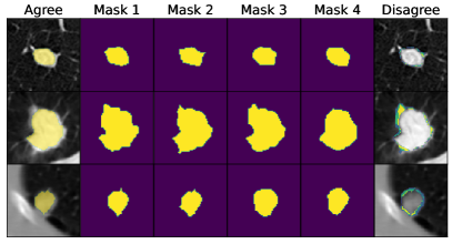
Figure 1: Samples of the LIDC-IDRI dataset with significant inter-observer variability where (dis-)agreement in the ground-truth masks is clearly visible.

Several deep learning architectures have been proposed for aleatoric uncertainty quantification. Presenting various plausible image segmentation hypotheses was initially enabled by the use of Monte-Carlo dropout [14, 15], ensembling methods [16, 17], or the use of multiple classification heads [18]. However, these methods approximate the weight distribution over the neural networks, i.e., the epistemic uncertainty, rather than the aleatoric uncertainty. Specifically, ensembling methods have been subject to criticism due to the lack of connection with Bayesian theory [19]. In this context, the PU-Net made significant advances by combining the conditional Variational Autoencoder (VAE) [20, 21] and U-Net [22]. In this case, a suitable objective is derived from the ELBO of the conditional data log-likelihood, which is analogous to the unconditional VAE. Nonetheless, several works have recently highlighted the limitations of the PU-Net [23, 24, 25]. Most relevant to this work, which pertains improving the latent space, is the augmentation of Normalizing Flows to the posterior density to boost expressivity[26, 27]. Also, Bhat et al. [28] demonstrate changes in model performance subject to density modeling design choices. Beyond this, the latent-space behaviour of the PU-Net has, to the best of our knowledge, not received much attention.

Therefore, this work explores the latent space of the PU-Net. We find that it can possess properties that inhibit aleatoric uncertainty quantification. Specifically, the learned latent space successfully represents the data variability by adjusting the latent-density variances required to encapsulate the information variability. Nevertheless, this affects the performance during both optimization and deployment. During training, the inhomogeneous latent variances cause the network to be ill-conditioned, resulting in inefficient and unstable gradient descent updates. At test time, the output is disproportionately sensitive to the localization of latent samples, which leads to erroneous segmentations. We find clear relationship between the homogeneity of the latent-density singular values and the ability to accurately encapsulate the inter-observer variability. Therefore, we suggest considering the problem from the perspective of Optimal Transport (OT), rather than data log-likelihood maximization. This enables the introduction of a new model, the Sinkhorn PU-Net (SPU-Net), which uses the Sinkhorn Divergence in the latent space. The proposed SPU-Net architecture distributes the latent variances more evenly over all dimensions by retaining variances of possibly non-informative latent dimensions, rather than directly minimizing them. As such, the decoder is better conditioned and gradient-descent optimization is significantly improved. Furthermore, the decoder is more robust to shifting latent densities, because the probability that the decoder receives unseen samples during test time is greatly reduced. To summarize, the contributions of this work are:

• Providing detailed insights into the effect of singular values on the quantification of aleatoric uncertainty with latent density models.

• Introducing the SPU-Net, which rephrases the optimization in the context of Optimal Transport, which thereby significantly improves (up to 11%) upon preceding latent variable models for probabilistic segmentation.

The remainder of this paper is structured as follows. First, we present various theoretical frameworks, which includes the Variational Autoencoder, Probabilistic U-Net and Optimal Transport in Section II. Consequently, the OT problem is phrased in the context of probabilistic segmentation. Additionally, training and evaluation of the SPU-Net is introduced in Section III. Quantitative and qualitative results are shown in Section IV. Limitations of our work are discussed in Section V and finally, conclusions are drawn in Section VI.

II Theoretical Background

This section provides an introduction to the VAE and PU-Net, where both models maximize the lower bound on the data log-likelihood. Additionally, the theory of Optimal Transport will be presented with the intention to enable the use of alternative divergence measures in latent space. In the remainder of this paper, we will use calligraphic letters ($\mathcal{X}$) for sets, capital letters ($X$) for random variables, and lowercase letters ($x$) for specific values. Furthermore, we will denote marginals as $P_{X}$, probability distributions as $P(X)$, and densities as $p(x)$. Vectors and matrices are distinguished with boldface characters. Notation for data manifolds and their probability measures have carefully been adapted from the works of Dai et al. [29] and Zheng et al. [30].

II-A Variational Autoencoders

Let $\mathbf{x}\in\mathcal{X}$ be an observable variable, taking values in $\mathbb{R}^{D}$. We define $\mathbf{z}\in\mathcal{Z}$ as a latent, lower-dimensional representation of $\mathbf{x}$, taking values in $\mathbb{R}^{d}$. It is assumed that $\mathcal{X}$ possesses a low-dimensional structure in $\mathbb{R}^{r}$, relative to the high-dimensional ambient space $\mathbb{R}^{D}$. Thus, it is assumed that $D\gg d\geq r$. In other words, the latent dimensionality $d$ is greater than the intrinsic dimensionality $r$ of the data. Let us also denote a ground-truth probability measure $\mu_{gt}$ on $\mathcal{X}$ such that $\int_{\mathcal{X}}\mu_{gt}(d\mathbf{x})=1$, where $\mu_{gt}(d\mathbf{x})$ pertains probability mass of infinitesimal $d\mathbf{x}$ on the manifold. The VAE [20] aims to approximate the data distribution through $\mathbf{z}$, by maximizing the Evidence Lower Bound (ELBO) on the data log-likelihood, described by

$$\log p(\mathbf{x}) \geq\mathbb{E}_{q_{\bm{\theta}}(\mathbf{z}|\mathbf{x})}\left[\log\frac{p(\mathbf{x},\mathbf{z})}{q_{\bm{\theta}}(\mathbf{z}|\mathbf{x})}\right]$$

$$\geq\mathbb{E}_{q_{\bm{\theta}}(\mathbf{z}|\mathbf{x})}\left[\log p_{\bm{\phi}}(\mathbf{x}|\mathbf{z})\right]$$

$$\qquad-\mathrm{KL}\left[q_{\bm{\theta}}(\mathbf{z}|\mathbf{x})\,||\,p(\mathbf{z})\right],$$ (1)

with tractable encoder $q_{\bm{\theta}}(\mathbf{z}|\mathbf{x})$ (commonly known as the posterior) and decoder $p_{\bm{\phi}}(\mathbf{x}|\mathbf{z})$ densities, amortized with parameters $\bm{\theta}$ and $\bm{\phi}$, respectively. Furthermore, $p(\mathbf{z})$ is a fixed latent density and is commonly referred to as the prior. As a consequence of the mean-field approximation, the densities are modeled with axis-aligned Normal densities. Furthermore, to enable prediction from test images, optimization is performed through amortization with neural networks. Nevertheless, due to these approximations, this construction can be sub-optimal, reduce the effectiveness of the VAE and void the guarantee that high ELBO values indicate accurate inference [31, 32].

It has been discussed in the work of Dai et al. [29] that the VAE is inclined to informative latent variances as much as possible while matching the non-informative variances to the prior to satisfy the KL-divergence. Because of this, the VAE is well-capable of learning the intrinsic dimensionality of the data. Nevertheless, the minimization of the latent variances induces an intrinsic bias. Namely, the VAE will progressively improve its approximation of the support of $\mu_{gt}$ on the manifold $\mathcal{X}$, while neglecting the probability measure itself. This has detrimental effects on the ancestral sampling capabilities of the VAE.

II-B The Probabilistic U-Net

Similar to the VAE, we can consider input image and ground-truth segmentation masks $\mathbf{x},\mathbf{y}\in\mathbb{R}^{D}$. Then, the ELBO of the conditional data log-likelihood can be written as

$$\log p(\mathbf{y}|\mathbf{x}) \geq\mathbb{E}_{q_{\bm{\theta}}(\mathbf{z}|\mathbf{x},\mathbf{y})}\left[\log\frac{p(\mathbf{y},\mathbf{z}|\mathbf{x})}{q_{\bm{\theta}}(\mathbf{z}|\mathbf{x},\mathbf{y})}\right]$$

$$\geq\mathbb{E}_{q_{\bm{\theta}}(\mathbf{z}|\mathbf{x},\mathbf{y})}\left[\log p_{\bm{\phi}}(\mathbf{y}|\mathbf{x},\mathbf{z})\right]$$

$$\qquad-\mathrm{KL}\left[q_{\bm{\theta}}(\mathbf{z}|\mathbf{x},\mathbf{y})\,||\,q_{\bm{\psi}}(\mathbf{z}|\mathbf{x})\right].$$ (3)

We denote the probability measure of the conditioning variable as $\nu_{gt}$, where $\int_{\mathcal{X}}\nu_{gt}(d\mathbf{x})=1$. For any $\mathbf{x}\in\mathcal{X}$ we have subset $\mathcal{Y}_{\mathbf{x}}\subseteq\mathcal{Y}$ containing probability measure $\omega^{\mathbf{x}}_{gt}$, with $\int_{\mathcal{Y}_{\mathbf{x}}}\omega^{\mathbf{x}}_{gt}(d\mathbf{y})=1$ and $\int_{\mathcal{X}\times\mathcal{Y}_{\mathbf{x}}}\omega^{\mathbf{x}}_{gt}(d\mathbf{y})\,\nu_{gt}(d\mathbf{x})=1$. The predictive distribution of $\mathbf{y}^{*}$ from test image $\mathbf{x}^{*}$ can be obtained with

$$p(\mathbf{y}^{*}|\mathbf{x}^{*}):=\int_{\mathbb{R}^{d}}p_{\bm{\phi}}(\mathbf{y}^{*}|\mathbf{z},\mathbf{x}^{*})q_{\bm{\psi}}(\mathbf{z}|\mathbf{x}^{*})d\mathbf{z},$$ (3)

and test segmentations are obtained with ancestral sampling.

The success of the PU-Net for probabilistic segmentation can be accredited to several additional design choices in the implementation of the encoding-decoding structure. Firstly, an encoding $\mathbf{z}$, is inserted pixel-wise at the final stages of a U-Net, followed by feature-combining 1$\times$1 convolutions only. As a result, this significantly alters the $r$-dimensional manifold that $\mathbf{z}$ attempts to learn. Namely, it learns the segmentation variability within a single image rather than features of the segmentation itself. Therefore, much smaller values of $d$ are feasible. An illustration of the (S)PU-Net is provided in Figure 2.

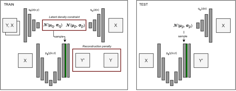
Figure 2: Schematic drawing of the Probabilistic U-Net training framework introduced by Kohl et al. [33], where the latent density constraint is purely KL-divergence. The architecture maximizes the Evidence Lower Bound of the conditional data log-likelihood. The ground truth is denoted as Y, the input image as X, and the model prediction as Y’. During testing, only the prior density $p_{\psi}(\mathbf{z}|\mathbf{x})$ is used to predict samples. Besides the KL-divergence, the SPU-Net additionally constrains the latent space with the Sinkhorn Divergence.

A crucial difference in the PU-Net formulation w.r.t. to that of the VAE is the conditioning of the prior $p_{\bm{\psi}}(\mathbf{z}|\mathbf{x})$, which is not fixed but rather learned. Although it has been argued by Zheng et al. [30] that learning the prior density is theoretically equivalent to using a non-trainable prior, their respective optimization trajectories can differ substantially such that the former method is preferred [33]. Consider the KL-divergence between two $d$-dimensional axis-aligned Normals $\mathcal{N}_{1}$ and $\mathcal{N}_{2}$ with identical mean

$$2\cdot\operatorname{KL}\left[\,\mathcal{N}_{1}\,||\,\mathcal{N}_{2}\,\right]=\sum_{i}\frac{\sigma^{i}_{2}}{\sigma^{i}_{1}}+\ln\frac{\sigma^{i}_{1}}{\sigma^{i}_{2}}-d.$$ (4)

Minimizing this expression entails finding $\sigma^{i}_{1}=\sigma^{i}_{2}$ for all values of $i$. At the same time, the singular values are progressively minimized [30] and the variance vectors $\bm{\sigma}_{1}$ and $\bm{\sigma}_{2}$ are not constrained in any fashion, and therefore arbitrarily distributed. This fact carries potentially detrimental implications for the decoder $p_{\bm{\phi}}(\mathbf{y}|\mathbf{x},\mathbf{z})$, as will be discussed in the next section.

II-C Decoder sensitivity

A potential issue that can arise when training the PU-Net occurs when the model converges to solutions where respective latent dimensions variances vary significantly in magnitude. Namely, it causes the decoder to become extremely sensitive to the latent-space sample localization. The PU-Net decoder is dependent on the function $\mathbf{f}_{\bm{{\phi}}}(\mathbf{x},\mathbf{z})$, where $p_{\bm{\phi}}(\mathbf{y}|\mathbf{x},\mathbf{z})=\delta(\mathbf{y}-\mathbf{f}_{\bm{{\phi}}}(\mathbf{x},\mathbf{z}))$, which intermediately involves latent variable $\mathbf{z}$ to reconstruct a plausible segmentation hypothesis. The latent variable $\mathbf{z}$ is controlled by the mean $\bm{\mu}$ and singular values $\bm{\sigma}$ of the underlying axis-aligned Normal density. If the input $\mathbf{x}$ is considered to be fixed, then the relative condition number, $\zeta_{i}$, of $\mathbf{f}_{\bm{{\phi}}}(\mathbf{x},\mathbf{z})$ can be interpreted as the sensitivity of its output w.r.t. its varying input $z_{i}$, corresponding to the $i$-th latent dimension, which can be expressed as

$$\zeta_{i}=\lim_{\epsilon\rightarrow 0}\sup_{||\delta z_{i}||\leq\epsilon}\frac{||\delta\mathbf{f}_{\bm{{\phi}}}(\mathbf{x},z_{i})||\;/\;||\mathbf{f}_{\bm{{\phi}}}(\mathbf{x},\mathbf{z})||}{||\delta z_{i}||\;/\;||\mathbf{z}||}.$$ (5)

For convenient notation, only the varying $z_{i}$ is included in $\delta\mathbf{f}_{\bm{{\phi}}}(\mathbf{x},z_{i})$ rather than the complete vector $\mathbf{z}$. The condition number of a function has direct consequences to the numerical stability of its gradient updates. Suppose $\sigma_{1}\gg\sigma_{2}$ and $\mu_{1}\approx\mu_{2}$, then $\zeta_{2}\gg\zeta_{1}$, and the function is said to be ill-conditioned. In turn, this skews the optimization landscape where the gradients w.r.t. $z_{2}$ will dominate, leading to inefficient and unstable gradient descent updates. When considering that the dimensionality is usually higher than $d=2$, the search towards an optimal minimum will rapidly suffer from irregular condition numbers [34]. For instance, normalization layers have been used in neural networks to smoothen the optimization landscape and have led to considerable improvements [35, 36, 37, 38, 39]. Hence, a mechanism that promotes uniform condition numbers will smoothen optimization and encourage similar performance gains. In the case of latent variable modeling, this pertains stimulating latent variances which are approximately of the same magnitude. We hypothesize that obtaining better gradient estimates can also encourage the model to more accurately model the ground-truth probability measure $\omega^{\mathbf{x}}_{gt}$.

During deployment of the model, another problem can occur due to inhomogeneous latent-space variances. As mentioned before, the prior density is learned through amortization. This implies that the prior should be able to sufficiently reflect the posterior during test time, such that the decoder receives samples similar to that during training. Undoubtedly, misalignment between the two densities is expected, potentially leading to low-probability samples from the prior. In the case of extreme difference between the respective posterior latent variances, a simple shift in prior density mean can already cause out-of-distribution samples. This implies the decoder receives latent codes which were completely unseen during training, which in turn can cause highly inaccurate to even nonsensical predictions. Ideally, changes in sample localization should minimally affect its probability on the posterior density. To achieve this robustness, the singular values of the latent densities should be as homogeneous as possible. We visualize this phenomena in Figure 3.

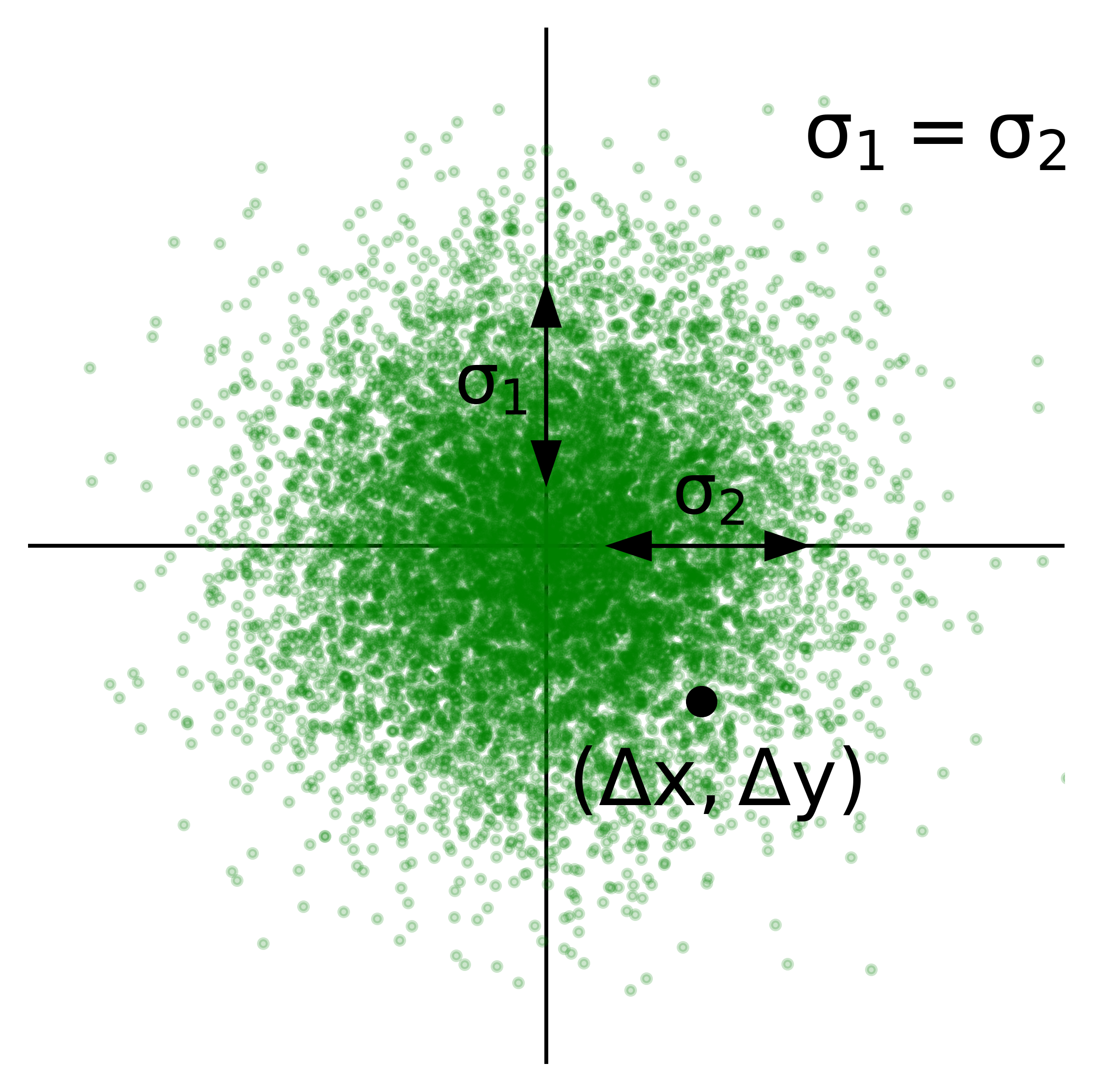
(a)

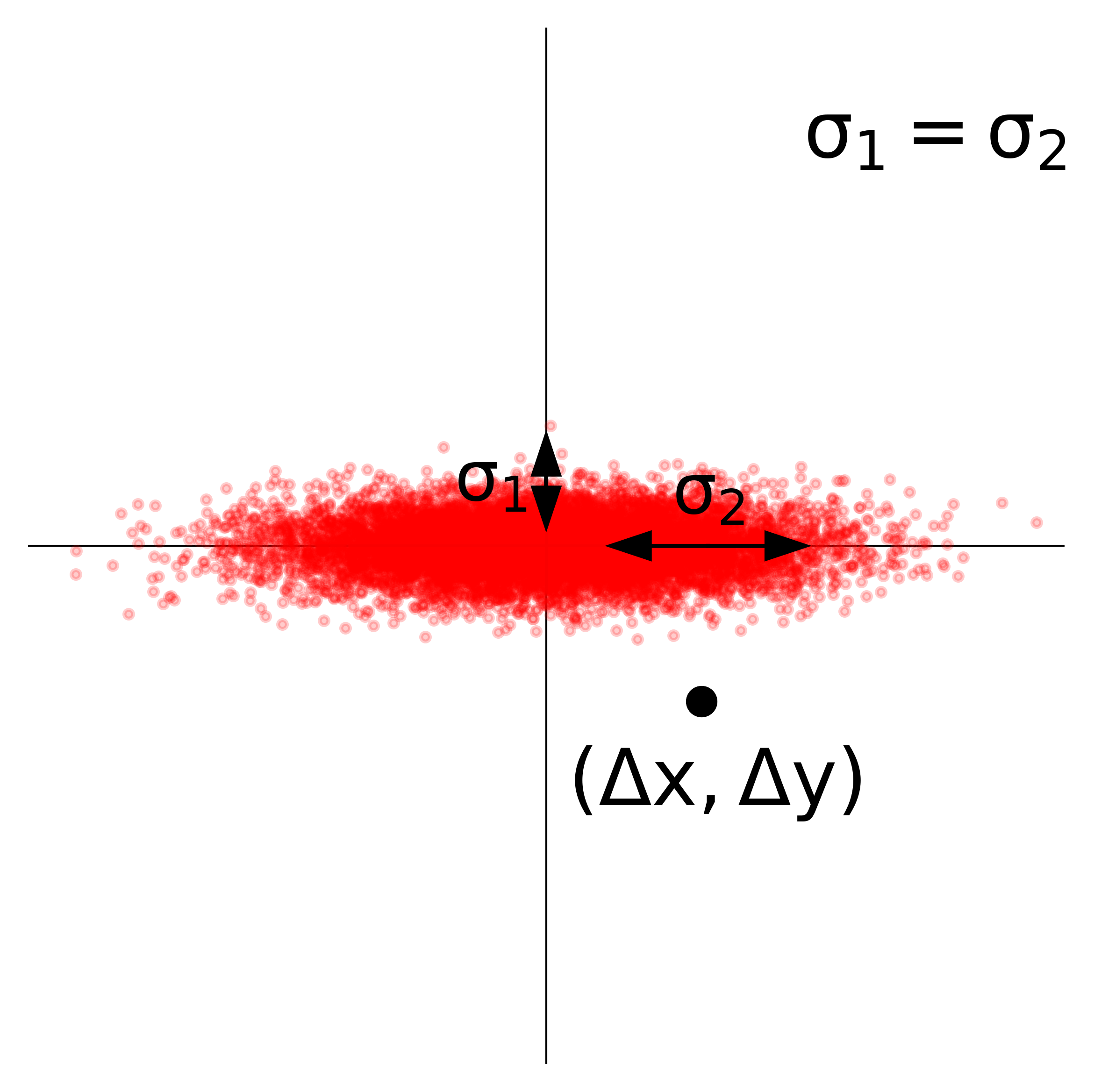
(b)

Figure 3: Axis-aligned Normal density singular values and its effect on decoder sensitivity. a) If the singular values are equal, then the decoding function is well-conditioned and robust to sample sensitivity. A slight shift in sample localization $(\Delta x,\Delta y)$ does not push the vector off the density support b) If the difference in relative magnitude of the singular values is significant, the decoding function is ill-conditioned and a slight shift in sample localization causes it to be completely out-of-distribution.

Furthermore, past literature has made mention of enhancing the posterior density by augmentation of Normalizing Flows [40], which was proposed to enhance the expressivity and complexity of the posterior distribution. This has shown to improve the PU-Net [26, 27]. Nevertheless, it has been argued in previous works that the mean-field Gaussian assumption in the VAE is not necessarily the cause for the failure to learn the ground-truth manifold [29]. Additionally, the complexity of the posterior density is limited by the Normally-distributed prior density, which will be used during testing. Thus, further exploration on the influence of the NF-augmented posterior on the prior density is required.

II-D Optimal Transport

This section provides an introduction to the Optimal Transport (OT) framework. Let $\mathcal{Y}$ and $\mathcal{\hat{Y}}$ be the two separable metric spaces. For the sake of clarity, the reader can assume that these sets contain the ground-truth and model predictions, respectively. We adopt the Monge-Kantorovich formulation [41] for the OT problem, by specifying

$$W(\mu,\hat{\mu} ):=$$

$$\operatorname{inf}\left\{\int_{\mathcal{Y}\times\mathcal{\hat{Y}}}c(\mathbf{y},\hat{\mathbf{y}})\,d\gamma(\mathbf{y},\hat{\mathbf{y}})\bigg{|}\gamma\in\Gamma(\mu,\hat{\mu})\right\},$$ (5)

where $\gamma\in\Gamma(\mu,\hat{\mu})$ denotes a coupling in the tight collection of all probability measures on $\mathcal{Y}\times\mathcal{\hat{Y}}$ with marginals $\mu$ and $\hat{\mu}$, respectively. The function $c(\mathbf{y},\hat{\mathbf{y}})$: $\mathcal{Y}\times\mathcal{\hat{Y}}\rightarrow\mathbb{R}_{+}$ denotes any lower semi-continuous measurable cost function. Equation (6) is also commonly referred to as the Wasserstein distance. Furthermore, the usual context of this formulation is in finding the lowest cost of moving samples from the probability measures in $\mathcal{Y}$ to the measures in $\mathcal{\hat{Y}}$. In the case of probabilistic segmentation, the aim is to learn the marginal ground-truth distribution $P_{Y,X}=\int p(\mathbf{y}|\mathbf{x})\mu_{gt}(d\mathbf{x})$, by matching it with the marginal model distribution $P_{\hat{Y},X}=\int p(\mathbf{\hat{y}}|\mathbf{x})\mu_{gt}(d\mathbf{x})$.

The Wasserstein distance is in practice a tedious calculation. As a solution, it has been proposed to introduce entropic regularization [42]. This is achieved by using the entropy of the couplings $\gamma$ as a regularizing function, which is specified by

$$\tilde{S}_{\epsilon}(\mu,\hat{\mu} ):=$$ (7)

$$\operatorname{inf}\bigg{\{}\int_{\mathcal{Y}\times\mathcal{\hat{Y}}}s(\mathbf{y},\mathbf{\hat{y})}d\gamma(\mathbf{y},\hat{\mathbf{y}})\bigg{|}\gamma\in\Gamma(\mu,\hat{\mu})\bigg{\}},$$

where

$$s(\mathbf{y},\mathbf{\hat{y}})=d(\mathbf{y},\mathbf{\hat{y}})+\epsilon\operatorname{log}\frac{d\gamma(\mathbf{y},\hat{\mathbf{y}})}{d\mu(\mathbf{y})d\hat{\mu}(\mathbf{\hat{y}})}.$$ (8)

As mentioned by Cuturi et al. [43], the entropy term can be expanded to $\operatorname{log}(d\gamma(\mathbf{y},\hat{\mathbf{y}}))-\operatorname{log}(d\mu(\mathbf{y}))-\operatorname{log}(d\hat{\mu}(\mathbf{\hat{y}}))$. In this way, this formulation can be understood as constraining the joint probability to have sufficient entropy, or contain small enough mutual information with respect to $d\mu$ and $d\hat{\mu}$. Cuturi et al. [43] show that this entropic regularization allows optimization over a Lagrangian dual for faster computation with the iterative Sinkhorn matrix scaling algorithm. Additionally, the entropic bias is removed from the OT problem to obtain the Sinkhorn Divergence, specified as

$$S_{\epsilon}(\mu,\hat{\mu})=\tilde{S}_{\epsilon}(\mu,\hat{\mu})-\frac{1}{2}\left(\tilde{S}_{\epsilon}(\mu,\mu)+\tilde{S}_{\epsilon}(\hat{\mu},\hat{\mu})\right).$$ (9)

The Sinkhorn Divergence interpolates between $W_{p}$ when $\epsilon\rightarrow~{}0$ with $\mathcal{O}(\epsilon\operatorname{log}(\frac{1}{\epsilon}))$ deviation, and Maximum Mean Discrepancy when $\epsilon\rightarrow\infty$, which favours dimension-independent sample complexity [44]. A viable option is to approximate the Sinkhorn Divergence via sampling with weights $\alpha,\beta\in\mathbb{R}_{+}$. The regularized Sinkhorn algorithm performance lacks in lower temperature settings. To alleviate this limitation, as well as to increase efficiency, Kosowsky and Yuille [45] introduce $\epsilon$-scaling or simulated annealing to the Sinkhorn algorithm.

Various works have investigated constraining the latent densities by means of Optimal Transport [46]. Tolstikhin et al. [47] introduce Wasserstein Autoencoders (WAEs), which softly constrain the latent densities with a Wasserstein penalty term, a metric that emerged from OT theory [48]. The authors demonstrate that the WAEs exhibit better sample quality while maintaining the favourable properties of the VAE. Similarly, Patrini et al. [49] introduce the Sinkhorn Autoencoder (SAE), in which the Sinkhorn algorithm [43] – an approximation of the Wasserstein distance – is leveraged as a latent divergence measure.

III Methods

It has been argued that the PU-Net can converge to sub-optimal latent representations. In this section, we introduce the SPU-Net, which uses the Sinkhorn Divergence between the conditional latent densities. The utilized entropic regularization can induce favourable latent properties for aleatoric uncertainty quantification.

III-A SPU-Net

By using the theoretical frameworks of Bousquet et al. [46], generative latent variable models can be trained from the perspective of OT. Most works employ this technique to provide an alternative to the conventional VAE objective [49, 47]. We specifically consider the optimization problem in the conditional setting for probabilistic segmentation and have framed previous literature accordingly to this context. Consequently, we can elegantly present an alternative training objective for the PU-Net.

Rather than maximizing the conditional data log-likelihood, the OT between the ground truth and model distributions is minimized. We consider the random variables $(X,Y,\hat{Y},Z)\in\mathcal{X}\times\mathcal{Y}\times\mathcal{\hat{Y}}\times\mathcal{Z}$, which correspond to the input image, ground-truth segmentation, model prediction and latent code, respectively. Then, we denote the joint distribution $P_{Y,Z,X}$ where a latent variable is obtained as $X\sim P(X)$ followed by $Z\sim P(Z|X)$, and ground truth is obtained with $Y\sim P(Y|Z,X)$. The OT problem considers couplings $\Gamma(Y,\hat{Y}|X)=\Gamma(\hat{Y}|Y,X)P(Y)$, where $\Gamma(\hat{Y}|Y,X)$ can be factored with a non-deterministic mapping through latent variable $Z$, as is shown by Bousquet et al. [46]. In fact, considering a probabilistic encoder $Q(Z|Y,X)$, deterministic decoder $f_{{\phi}}$ and the set of joint marginals $\mathcal{P}_{Y,Z,X}$, the optimal solution of the OT problem can be stated as

$$W(P_{Y},P_{\hat{Y}})=\inf_{P\in\mathcal{P}_{Y,Z,X}}\mathbb{E}_{P_{Y,Z,X}}\left[c(Y,f_{\bm{\phi}}(Z,X)\right]$$ (10a)

$$=\inf_{\mathcal{Q}:Q_{Z}=P_{Z}}\mathbb{E}_{P_{Y,X}}\mathbb{E}_{Z\sim Q}\left[c(Y,f_{\bm{\phi}}(Z,X)\right]$$ , (10b)

with induced aggregated prior and posterior, $P_{Z}~{}=~{}\mathbb{E}_{P_{X}}\left[P(Z|X)\right]$ and $Q_{Z}~{}=~{}\mathbb{E}_{P_{Y,X}}\left[Q(Z|Y,X)\right]$, respectively (see Theorem 1 of Bousquet et al. [46] for further details). Equation (10a) follows by definition and Equation (10b) indicates that this search can be factored through a probabilistic encoder, which attempts to match the marginal $P_{Z}$. In this context, the optimization runs over probabilistic encoders $\mathcal{Q}$ rather than the couplings $\Gamma$. Continuously, the constraint on the aggregated marginals can be relaxed with a convex penalty $D:\mathcal{Q}\times\mathcal{P}\rightarrow\mathbb{R}_{+}$ such that $D(Q_{Z},P_{Z})=0$ if, and only if $Q_{Z}=P_{Z}$. Tolstikhin et al. [47] demonstrate that when choosing $D$ to be p-Wasserstein, defined as

$$W_{p} (Q_{\mathrm{Z}},P_{\mathrm{Z}}):=$$

$$\operatorname{inf}\left\{\left(\int_{\mathcal{Q}\times\mathcal{P}}d(\mathbf{q},\mathbf{p})^{p}\,d\gamma(\mathbf{q},\mathbf{p})\right)^{\frac{1}{p}}\bigg{|}\gamma\in\Gamma(Q_{\mathrm{Z}},P_{\mathrm{Z}})\right\},$$ (11)

the following equality can be established

$$W(P_{\mathrm{Y}},P_{\mathrm{\hat{Y}}})=\underset{Q\in\mathcal{Q}}{\operatorname{inf}}\sqrt[p]{\mathbb{E}_{P_{Y,X}}\mathbb{E}_{\mathrm{Z}\sim Q}[c(\mathrm{Y},f_{\bm{\phi}}(Z,X))^{p}]}$$

$$+\delta\cdot W_{p}(Q_{\mathrm{Z}},P_{\mathrm{Z}}),$$ (12)

where $f_{\phi}$ is at least $\delta$-Lipschitz. We highlight the importance of this continuity requirement, because it is directly related to the sensitivity of $f_{\phi}$, and thus the effectiveness of gradient descent methods. Patrini et al. [49] make use of the Sinkhorn iterations to approximate $W_{p}$. We adopt this strategy to encourage full utilization of the latent space, with the hypothesis that this property will improve the condition number of the posterior. In turn, this will decrease probability of unlikely samples due to inaccurate prior-density estimates during testing and possibly improve estimation of ground-truth probability measure. As a consequence, the model is overall more robust and defective predictions are prevented.

When using OT solutions, constraining the localization of the prior latent samples is important. A valid option is to subject the samples to a characteristic kernel, which is restricted to Reproducible Kernel Hilbert Space. However, to respect the flexible nature of the parameterized prior density, we simply constrain by means of an additional KL-divergence term. To deal with a varying number of annotations, we constrain the individual posteriors as an approximation to the divergence of the aggregated densities. This also enables random sampling of ground-truth masks, which has shown to be effective when dealing with multi-annotated data [33, 9]. As a result, the minimization objective of the SPU-Net can be stated as

$$\mathcal{L}=-\mathbb{E}_{q_{\bm{\theta}}(\mathbf{z}|\mathbf{x},\mathbf{y})} \left[\log p_{\bm{\phi}}(\mathbf{y}|\mathbf{x},\mathbf{z})\right]$$

$$+\alpha\cdot\mathrm{S}_{\epsilon} \left[q_{\bm{\theta}}(\mathbf{z}|\mathbf{x},\mathbf{y})\,||\,p_{\bm{\psi}}(\mathbf{z}|\mathbf{x})\right]$$

$$+\beta\,\cdot\, \mathrm{KL}\left[q_{\bm{\theta}}(\mathbf{z}|\mathbf{x},\mathbf{y})\,||\,p_{\bm{\psi}}(\mathbf{z}|\mathbf{x})\right],$$ (13)

where $\alpha$ and $\beta$ are tunable parameters.

III-B Data

This study employs a diverse range of post-processed, multi-annotated medical image segmentation datasets, which exhibit significant variations in the ground truth, to train and evaluate the proposed models. The utilization of publicly available datasets in this research underscores the clinical significance and the imperative for models to capture the inherent ambiguity present within these images. Firstly, we use the LIDC-IDRI [50] dataset, a popular benchmark for aleatoric uncertainty quantification, which contains lung-nodule CT scans. Secondly, we use the Pancreas and Pancreatic-lesion CT datasets and, finally, the Prostate and Brain-growth MRI datasets provided by the QUBIQ 2021 Challenge[51]. See Table I for more details on these datasets. It is assumed that the region of interest is detected and the desired uncertainty is solely regarding its exact delineation. Therefore, each image is center-cropped to 128$\times$128-pixel patches. Furthermore, a train/validation/test set is exploited where approximately 20% of the dataset is reserved for testing and three-fold cross-validation is used on the remaining 80%. We carefully split the data according to patient number to avoid data leakage or model bias.

Dataset		Modality	# readers	# images
LIDC-IDRI		CT	$4$	$15096$
QUBIQ	Pancreas	CT	$2$	$869$
	Pancreatic lesion	CT	$2$	$238$
	Prostate	MRI	$6$	$52$
	Brain growth	MRI	$7$	$39$

TABLE I: Details on the modality, and number of readers and images of the used datasets.

III-C Training

The proposed SPU-Net is compared to the PyTorch implementation of the PU-Net [33] and its NF-augmented variant (with a 2-step planar flow) [26], which we will refer to as the PU-Net+NF. We point readers to the respective papers for further details on both the PU-Net and PU-Net+NF architectures. Our code implementation of the SPU-Net is publicly available.

For each particular dataset, we train the PU-Net, PU-Net+NF and SPU-Net. Each of those models are trained on three folds using cross-validation. Furthermore, the experiments per model and dataset are conducted across four latent dimensions. All hyperparameters across experiments are kept identical, except for the number of training epochs and parameters related to the Sinkhorn Divergence. This implies across all datasets an $\alpha$ and $\beta$ set at $10$, a batch size of $32$, using the Adam optimizer with a maximum learning rate of $10^{-4}$ that is scheduled by a warm-up and cosine annealing, and weight decay of $10^{-5}$. For the LIDC-IDRI dataset we set the number of training epochs to 200 and for all QUBIQ datasets we trained for 2,500 epochs. After training, we used the model checkpoint with the lowest validation loss. This was usually much earlier than the set number of iterations. Additionally, we found that clipping the gradient to unitary norm was essential for the SPU-Net. To implement the Sinkhorn Divergence, we make use of the GeomLoss [52] package. Also, data augmentation has been used during training, which consisted of random rotation, translation, scale and shears.

III-D Evaluation

III-D1 Data distribution

To evaluate the model performances, Hungarian Matching has recently been used as an alternative to the Generalized Energy Distance (GED). This, because the GED can be biased to simply reward sample diversity when subject to samples of poor quality [24, 26]. We refer to Hungarian Matching as the Empirical Wasserstein Distance, abbreviated as EWD or $\hat{W}_{k}$, since it is essentially equivalent to the Wasserstein distance between the discrete set of samples from the model and the ground-truth distribution. Hence, the EWD is a well-suited metric, since the latent samples are attempted to be matched in a similar fashion as when using the Sinkhorn Divergence.

We implement the EWD as follows. Each set of ground-truth segmentations are multiplied to match the number of predictions $N$ obtained during testing. We then apply a cost metric $k$ to each combination of elements in the ground-truth and prediction set, to obtain an $N\times N$ cost matrix. Subsequently, the unique optimal coupling between the two sets that minimizes the average cost is determined. We use unity minus the Intersection over Union (1 - IoU) as cost function for $k$. We assign maximum score for correct empty predictions, which implies zero for the EWD. During test time, we sample 16 predictions for the LIDC-IDRI, Pancreas and Pancreatic-lesion dataset, 18 predictions for the Prostate and 21 predictions for the Brain-growth dataset, which were specifically chosen to be multiples of the number of available annotations.

III-D2 Latent distribution

To concretely measure inhomogeneous latent singular values of the prior density, one can consider two perspectives. In both cases, the acquisition of the singular value vector $\bm{\sigma}=[\sigma_{1},\sigma_{2},...,\sigma_{d}]$ is required. Since the densities are axis-aligned Normals, $\bm{\sigma}$ can be directly obtained from the diagonal of the covariance matrix and Singular Value Decomposition is not required. The first method uses $\bm{\sigma}$ to determine the Effective Rank (ER) [53] of the covariance matrix, which can be regarded as an extension of the conventional matrix rank. Hurley et al. [54] argue that entropy-based metrics, such as the ER, are sub-optimal as a sparsity measure according to their posed criteria. A different perspective indicates that a poor latent space is essentially a sparse $\bm{\sigma}$. Instead, the authors indicate that the Gini Index (GI) is more appropriate to quantify sparsity. Therefore, the Gini index, which is calculated with

$$\operatorname{GI}(\bm{\sigma})=1-2\sum_{k=1}^{d}\frac{\sigma_{k}}{\|\bm{\sigma}\|_{1}}\left(\frac{d-k+\frac{1}{2}}{d}\right),$$ (13)

will be used to evaluate the latent-space homogeneity.

IV Results & Discussion

Dataset	Model	$\mathbf{d=4}$		$\mathbf{d=5}$		$\mathbf{d=6}$		$\mathbf{d=7}$
		$\hat{W}_{k}\downarrow$	Gini$\downarrow$	$\hat{W}_{k}\downarrow$	Gini$\downarrow$	$\hat{W}_{k}\downarrow$	Gini$\downarrow$	$\hat{W}_{k}\downarrow$	Gini$\downarrow$
LIDC-IDRI	PU-Net	$0.451\pm 0.001$	$0.65\pm 0.01$	$0.450\pm 0.003$	$0.70\pm 0.01$	$0.451\pm 0.006$	$0.71\pm 0.01$	$0.451\pm 0.002$	$0.76\pm 0.02$
	PU-Net+NF	$0.451\pm 0.004$	$0.39\pm 0.08$	$0.450\pm 0.002$	$0.44\pm 0.11$	$0.446\pm 0.003$	$0.57\pm 0.07$	$0.450\pm 0.002$	$0.52\pm 0.05$
	SPU-Net	$0.440\pm 0.002$	$0.25\pm 0.03$	$0.440\pm 0.004$	$0.22\pm 0.01$	$\mathbf{0.439\pm 0.003}$	$0.38\pm 0.03$	$0.443\pm 0.004$	$0.45\pm 0.01$
QUBIQ Pancreas	PU-Net	$0.602\pm 0.034$	$0.64\pm 0.02$	$0.608\pm 0.024$	$0.74\pm 0.03$	$0.603\pm 0.030$	$0.78\pm 0.03$	$0.589\pm 0.002$	$0.80\pm 0.02$
	PU-Net+NF	$0.581\pm 0.004$	$0.52\pm 0.04$	$0.610\pm 0.080$	$0.49\pm 0.07$	$0.585\pm 0.021$	$0.61\pm 0.04$	$0.589\pm 0.054$	$0.55\pm 0.11$
	SPU-Net	$\mathbf{0.540\pm 0.030}$	$0.28\pm 0.06$	$0.581\pm 0.016$	$0.44\pm 0.04$	$0.551\pm 0.021$	$0.45\pm 0.01$	$0.564\pm 0.028$	$0.28\pm 0.03$
QUBIQ Pancreatic lesion	PU-Net	$0.628\pm 0.009$	$0.72\pm 0.01$	$0.606\pm 0.004$	$0.78\pm 0.00$	$0.618\pm 0.002$	$0.83\pm 0.00$	$0.611\pm 0.007$	$0.82\pm 0.02$
	PU-Net+NF	$0.536\pm 0.024$	$0.48\pm 0.06$	$0.559\pm 0.022$	$0.46\pm 0.05$	$0.568\pm 0.063$	$0.58\pm 0.03$	$0.535\pm 0.025$	$0.44\pm 0.06$
	SPU-Net	$0.528\pm 0.012$	$0.22\pm 0.06$	$0.540\pm 0.023$	$0.24\pm 0.07$	$\mathbf{0.503\pm 0.026}$	$0.54\pm 0.04$	$0.524\pm 0.022$	$0.38\pm 0.03$
QUBIQ Prostate	PU-Net	$0.178\pm 0.014$	$0.20\pm 0.15$	$0.167\pm 0.005$	$0.38\pm 0.027$	$0.185\pm 0.008$	$0.32\pm 0.02$	$0.174\pm 0.007$	$0.34\pm 0.09$
	PU-Net+NF	———	———	$0.170\pm 0.007$	$0.27\pm 0.03$	———	———	———	———
	SPU-Net	———	———	$\mathbf{0.158\pm 0.005}$	$0.20\pm 0.08$	———	———	———	———
QUBIQ Brain Growth	PU-Net	$0.294\pm 0.006$	$0.19\pm 0.04$	$0.304\pm 0.014$	$0.21\pm 0.03$	$0.292\pm 0.015$	$0.25\pm 0.06$	$0.281\pm 0.009$	$0.35\pm 0.01$
	PU-Net+NF	———	———	———	———	———	———	$0.295\pm 0.011$	$0.29\pm 0.12$
	SPU-Net	———	———	———	———	———	———	$\mathbf{0.277\pm 0.012}$	$0.23\pm 0.04$

TABLE II: Comparison of the experimented models on various datasets. The PU-Net is re-implemented from [33] and PU-Net+NF from [26]. Results are evaluations on the test set. The mean and standard deviations (threefold cross-validation) of the Empirical Wasserstein metric with kernel unity minus the Intersection over Union (1-IoU) are presented. Furthermore, the homogeneity of the latent singular values are expressed with the Gini index. A clear relationship between a homogeneous latent space and model performance is visible.

To validate our implementation of the baseline, we have conducted a GED evaluation on the PyTorch implementation of the PU-Net. When evaluating the PU-Net using the LIDC-IDRI dataset, we have obtained GED values of 0.327$\,\pm\,$0.003, which closely align with the reported values in the work of Kohl et al. [24], yet exhibit significantly reduced standard deviation. Moreover, the Hungarian-Matched IoU values surpass the values reported by Kohl et al. [24]. These discrepancies can be potentially attributed to differences in training splits and model initialization. Nonetheless, these findings underscore the comparable performance of our experiments, warranting a reliable basis for accurate comparisons.

The quantitative results from the conducted experiments are presented in Table II. Optimal values for $d$ are found to reside within the range of 4 $\leq$ $d$ $\leq$ 7. For each dataset, the best performing model across the experimented latent dimensionalities are indicated in boldface. It can immediately be observed that the SPU-Net is the best performing model within and across each latent dimensionality in terms of aleatoric uncertainty quantification (visible from the EWD metric). Additionally, a positive correlation is apparent between the latent space homogeneity (GI) and EWD. The SPU-Net evenly distributes all variances of each latent dimensionality, which results in the best performance in terms of the EWD. This is in contrast to the PU-Net, which has a sparse latent space (i.e. high GI) and generally performed worse. The results for the PU-Net+NF support this empirical correlation as well, since its metric evaluations often reside between the former two in terms of both performance and latent space sparsity.

It is generally known that both PU-Net and PU-Net+NF utilize values of $d$ higher than the intrinsic inter-observer variability in the data. If the SPU-Net more appropriately deals with the latent dimensions, it can outperform the other two models with a smaller value of $d$, even if the latter model has the potential to encapsulate more information. Interestingly, this case is apparent in our quantitative results. The SPU-Net often performs better with a lower latent dimensionality than the PU-Net with larger values of $d$. A good example is found in the Pancreas dataset evaluations. For the PU-Net, the best results are found for $d$ = 7, while better performance is observed with significantly lower value ($d$ = 4). This observation challenges the idea that tuning the latent dimensionality implies finding the inherent $r$-dimensional manifold. For reasons yet unknown, the results suggests a strong indication that the uninformative dimensions are required to reach the best possible performance in the PU-Net. This is possibly due to the parameterized prior density, which can be theoretically fixed. Nonetheless, it is clear that homogenizing the latent variances improves its impact on model performance, which incurs it to outperform the PU-Net, regardless of the setting of hyperparameter $d$. Additionally, on the Pancreatic-lesion dataset, it is apparent that the SPU-Net outperforms the PU-Net+NF ($d$ = 7) with a smaller latent dimension ($d$ = 5). These findings further support the claim that a more homogeneous latent space improves model performance.

To further investigate the effect of latent-space sparsity on model performance, we have tracked the Gini index behaviour during model training. This is visualized for experiments with optimal values of $d$ with respect to the SPU-Net, and can be observed in Figure 4. At first glance, it is clear that the Prostate and Brain-growth datasets result in different behaviour compared to the other datasets. This can be due to the different acquisition methods (i.e. MRI) or the fact that the datasets are substantially smaller in size. Specifically for the Brain-growth dataset, this difference can be accredited also to the channel-wise concatenation of three imaging modalities, rather than inference with a single-channel input. Therefore, we initially shift our focus for this analysis to the LIDC-IDRI, Pancreas and Pancreatic-lesion datasets.

It is clear that all three models are subject to some volatility in the Gini index during early-stage training. This can range from a simple draw-down to several fluctuations. In Figure 4, it can be noticed that the SPU-Net (green) rapidly declines to a homogeneous latent representation thereafter, while the PU-Net (red) remains relatively sparse (i.e. high Gini index). Also, it can be noted that the volatility is generally more intense for the PU-Net+NF (blue) model and more time is required to reach a stable Gini index. We attribute these findings to the addition of an NF to the posterior density that introduces stochasticity, due to a nonclosed-form KL-divergence. Whereas the augmented NF increases posterior expressivity, the additional stochasticity in training inhibits effective optimization. However, the SPU-Net has the benefit of more appropriate latent space modeling as well as a closed-form KL-divergence for stable training.

Given that stochasticity during training is undesired, it is important that volatility is low and has a short duration, which will cause smoother gradients and better loss landscapes. Two specific cases can be observed with the Pancreas dataset in Table II that effectively demonstrate this undesired volatility. Thus, the Gini indices for these two datasets are depicted over the first training quartile in Figure 5. In the case of $d$ = 5, it can be seen that the PU-Net+NF model has a similar Gini index to that of the SPU-Net. However, the performance is much worse. This is because PU-Net+NF has a more significant drop-down than the SPU-Net, leading to unstable gradient-descent updates. For the case of $d$ = 7, the PU-Net and PU-Net+NF have similar performance even though their Gini indices vary significantly. Here, the volatility causes the PU-Net+NF to perform just as poor as the PU-Net, regardless of having a lower Gini index. These results further establish that the volatility during early-stage training inhibits effective gradient descent.

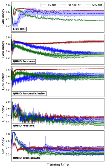
Figure 4: The Gini indices (lower is better) of the prior distribution during the 1st training quartile. The models differ with respect to each other according to two elements. Namely, the volatility in early-stage training and the eventual converged value.

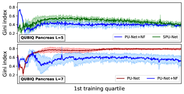
Figure 5: The Gini indices of the prior distribution during training. For the Pancreas dataset, it can be seen that the values corresponding to the PU-Net+NF model are more volatile in the early stages of training compared to the other two datasets.

Applying the aforementioned analysis to the Prostate and Brain-growth datasets is less reliable, since their training curves in Figure 4 significantly coincide. It should be noticed that the PU-Net+NF is worse than the PU-Net for both datasets. We hypothesize that this is related to the early-stage volatility of the Gini index. However, this is not immediately clear and is difficult to confirm from the figures.

To better understand the distribution of the latent dimensions, the means and variances of the image-conditional prior densities are depicted in Figure 6. Here, it can be clearly seen that the PU-Net is modeling the ambiguity on a very sparse latent representation. The PU-Net+NF better distributes this, which improves the conditioning of the decoder. More specifically, previous works have argued that the augmentation of NFs results in a more complex and expressive posterior. Our results show that the introduced technique regularizes the relative condition numbers of the decoder by stretching the non-informative latent variances. In the context of the gradient descent, we can consider augmenting with NFs as a form of preconditioning, where it smoothens the optimization by an appropriate transformation on the latent samples. Even though the NF-augmented posterior density can adapt many shapes, we have observed in the conducted experiments that the posterior density only slightly deviates from an axis-aligned Normal density. This is because the PU-Net+NF is still constrained by the Gaussian nature of the prior density. Therefore, the effect of an improved posterior approximation does not manifest beyond a prior with latent space of reduced sparsity. Finally, in line with the previously discussed results, it can be concluded the SPU-Net has the most homogeneous prior latent density.

The quantitative evaluation confirms the superior performance of the SPU-Net. Nevertheless, the model deployment in clinical settings will mainly entail visual evaluation. Therefore, we qualitatively inspect the means and standard deviations of the sampled predictions of the (S)PU-Net in Figures 7, 8, 9, 10 and 11. Notably, across all the datasets it can be observed that the SPU-Net more accurately delineates the uncertain areas (comparing the ground truth to the std. dev. column) of the lesion and is less prone to defective segmentations. These results further confirm our hypothesis that the latent space of the PU-Net is unfavourable. Specifically, the decoder is too sensitive to small shifts in latent-sample localization. During test time, the predicted prior density is often misaligned with the restrictive posterior manifold and therefore, the decoder receives very unlikely or even unseen samples. As a consequence, defective reconstructions are produced. For example, in the LIDC-IDRI dataset (Figure 7), it can be observed that some samples are empty, although there is obvious presence of a malicious lesion. In the QUBIQ Pancreas, Pancreatic-lesion and prostate predictions (Figures 8, 9 and 10) severe defects occur surrounding the areas of interest. It is very clear that the SPU-Net does not predict these defects. This is because its learned posterior manifold is stretched, which causes the decoder to be more robust to sample shift. The respective difference between the two models in the QUBIQ brain-growth dataset (Figure 11) is less apparent. Even though both models are free from severe misclassifications, under closer inspection it can be noticed that the uncertainty is modeled more accurately. This suggests that the model is not only more robust, but seems to have learned a more accurate probability measure.

In a similar vain, segmentation techniques with different approaches have been introduced as well [55, 56, 57]. In particular, Denoising Diffusion Probabilistic Models (DDPMs) have recently received substantial attention [58, 59, 60, 61, 62, 63, 64, 65]. Even though the segmentation results of DDPMs are promising, the inference procedure is extremely slow. This is especially cumbersome when sampling multiple predictions in uncertainty quantification. Additionally, modeling the ambiguity in latent space is a more natural approach, since the uncertainty in latent space is interpretable and semantically more relevant in contrast to pixel-level modeling. For example, this gives an opportunity to dissect components of the uncertainty that relate to image localization or annotation style. Furthermore, latent-variable modeling can aid in learning the lower-dimensional manifold intrinsic in the data, which can assist further development in more efficient compression-based algorithms.

To conclude, our results indicate sub-optimal latent spaces of the PU-Net(+NF). Namely, the PU-Net learns a restrictive manifold that minimizes the variances of the non-informative latent dimensions. While accurately estimating data manifolds can generally be seen as a desired property, we have found that this causes the decoder to become ill-conditioned, due to the highly inhomogenous latent variances. Another consequence is that the decoder becomes extremely sensitive to sample localization and can cause many erroneous predictions. The PU-Net+NF is able to alleviate this by learning more homogeneous latent variances. However, after inspection of both the qualitative and quantitative results, it is clear that the SPU-Net more effectively circumvents this issue with superior performance in uncertainty quantification. The results also suggest that thanks to this property, the estimated probability measure within the learned manifold can improve as well.

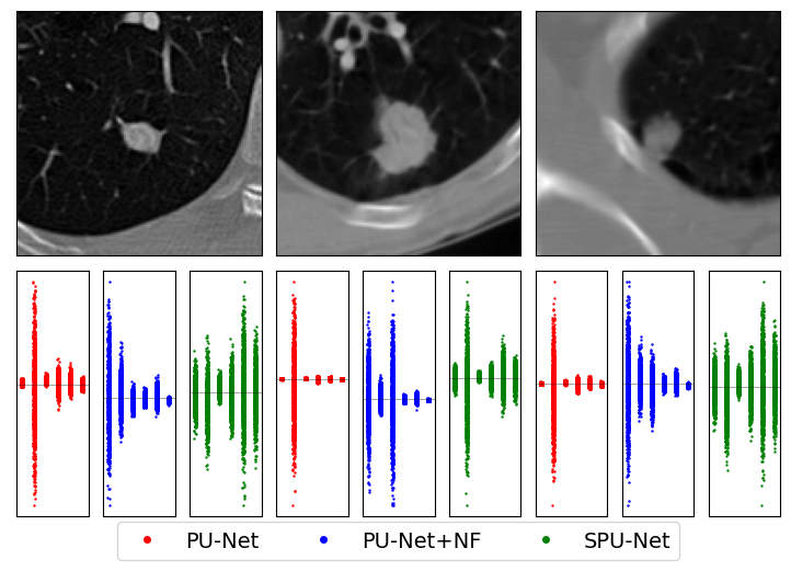
Figure 6: LIDC-IDRI variances.

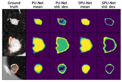
Figure 7: LIDC-IDRI test samples.

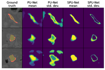
Figure 8: QUBIQ pancreas test samples.

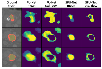
Figure 9: QUBIQ pancreatic lesion test samples,

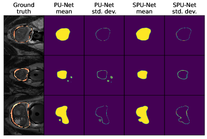
Figure 10: QUBIQ prostate test samples.

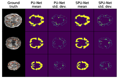
Figure 11: QUBIQ brain growth test samples.

V Limitations

This work is subject to several limitations. First, this research proposes to leverage the entropic regularization of the Sinkhorn iterations to prevent the latent dimensions from collapsing to minimal variance. However, adequate analysis has not yet been provided beyond this statement. It is important to understand which element of the entropic regularization contributes towards obtaining the desired latent space, so that further progress can be made in developing latent-density models. Secondly, this work attributes the resulting restrictive latent manifold to the KL-constraint in the ELBO formulation. However, this term still remains in the training objective. Experiments with an alternative for the KL-divergence should be provided to explore if additional performance gains are possible. Finally, the SPU-Net circumvents the requirement of comparing the aggregated prior and posterior to enable random sampling from the data and retain a simplified training procedure. Nevertheless, additional experimentation should be conducted with aggregated densities to achieve an architecture closer to the Wasserstein objective.

VI Conclusion

In this work, we have evaluated the Probabilistic U-Net on several multi-annotated datasets and have found that the performance is significantly inhibited due to the nature of the latent space. More specifically, it is shown that training the Probabilistic U-Net results in severely inhomogeneous singular values of the Normal latent densities that cause the model to become ill-conditioned and extremely sensitive to latent-sample localization. To alleviate this issue, we have introduced the Sinkhorn PU-Net (SPU-Net) that encourages uniform latent space variances, which results in a more robust model and improves probabilistic image segmentation for aleatoric uncertainty quantification. For future work, this research will be applied to multi-resolution probabilistic segmentation models, which similarly model the uncertainty in latent densities with the purpose to surpass state-of-the-art performance. This research paves way for improved uncertainty quantification for image segmentation in the medical domain, thereby assisting clinicians with surgical planning and patient care. Nevertheless, this work is by definition limited to segmentation or the medical domain. Other fields that aim to encapsulate data variability in latent densities can benefit from this research as well.

References

- [1] A. Kendall and Y. Gal, “What uncertainties do we need in bayesian deep learning for computer vision?,” NeurIPS, vol. 30, 2017.
- [2] A. S. Becker, K. Chaitanya, K. Schawkat, U. J. Muehlematter, A. M. Hötker, E. Konukoglu, and O. F. Donati, “Variability of manual segmentation of the prostate in axial t2-weighted mri: A multi-reader study,” European Journal of Radiology, vol. 121, p. 108716, 2019.
- [3] B. H. Menze et al., “The multimodal brain tumor image segmentation benchmark (brats),” IEEE TMI, vol. 34, no. 10, pp. 1993–2024, 2015.
- [4] A. Jungo, R. Meier, E. Ermis, M. Blatti-Moreno, E. Herrmann, R. Wiest, and M. Reyes, “On the effect of inter-observer variability for a reliable estimation of uncertainty of medical image segmentation,” in MICCAI, pp. 682–690, Springer, 2018.
- [5] S. K. Warfield, K. H. Zou, and W. M. Wells, “Simultaneous truth and performance level estimation (staple): an algorithm for the validation of image segmentation,” IEEE TMI, vol. 23, no. 7, pp. 903–921, 2004.
- [6] S. Vdineanu, D. Pelt, O. Dzyubachyk, and J. Batenburg, “An analysis of the impact of annotation errors on the accuracy of deep learning for cell segmentation,” in Medical Imaging with Deep Learning, 2021.
- [7] F. van der Sommen, S. Zinger, E. J. Schoon, et al., “Sweet-spot training for early esophageal cancer detection,” in Medical Imaging 2016: Computer-Aided Diagnosis, vol. 9785, pp. 330–336, SPIE, 2016.
- [8] J. van der Putten, F. van der Sommen, J. de Groof, M. Struyvenberg, S. Zinger, W. Curvers, E. Schoon, J. Bergman, et al., “Modeling clinical assessor intervariability using deep hypersphere encoder–decoder networks,” Neural Computing and Applications, vol. 32, no. 14, pp. 10705–10717, 2020.
- [9] T. G. Boers, C. H. Kusters, K. N. Fockens, J. B. Jukema, M. R. Jong, J. de Groof, J. J. Bergman, F. van der Sommen, and P. H. de With, “Comparing training strategies using multi-assessor segmentation labels for barrett’s neoplasia detection,” in CaPTion 2022, Held in Conjunction with MICCAI, Proceedings, pp. 131–138, 2022.
- [10] L. Joskowicz, D. Cohen, N. Caplan, and J. Sosna, “Inter-observer variability of manual contour delineation of structures in ct,” European radiology, vol. 29, no. 3, pp. 1391–1399, 2019.
- [11] T. Watadani, F. Sakai, T. Johkoh, S. Noma, M. Akira, K. Fujimoto, A. A. Bankier, K. S. Lee, N. L. Müller, J.-W. Song, et al., “Interobserver variability in the ct assessment of honeycombing in the lungs,” Radiology, vol. 266, no. 3, pp. 936–944, 2013.
- [12] E. Versteijne, O. J. Gurney-Champion, A. van der Horst, E. Lens, M. W. Kolff, J. Buijsen, G. Ebrahimi, K. J. Neelis, C. R. N. Rasch, J. Stoker, M. B. van Herk, A. Bel, and G. van Tienhoven, “Considerable interobserver variation in delineation of pancreatic cancer on 3dct and 4dct: a multi-institutional study,” Radiation Oncology (London, England), vol. 12, 2017.
- [13] I. Joo, J. M. Lee, E. S. Lee, J. Y. Son, D. H. Lee, S. J. Ahn, W. Chang, S. M. Lee, H.-J. Kang, and H. K. Yang, “Preoperative ct classification of the resectability of pancreatic cancer: Interobserver agreement.,” Radiology, p. 190422, 2019.
- [14] I. Osband, C. Blundell, A. Pritzel, and B. Van Roy, “Deep exploration via bootstrapped dqn,” NeurIPS, vol. 29, 2016.
- [15] B. Lakshminarayanan, A. Pritzel, and C. Blundell, “Simple and scalable predictive uncertainty estimation using deep ensembles,” NeurIPS, vol. 30, 2017.
- [16] C. Rupprecht, I. Laina, R. DiPietro, M. Baust, F. Tombari, N. Navab, and G. D. Hager, “Learning in an uncertain world: Representing ambiguity through multiple hypotheses,” in Proceedings of the ICCV, pp. 3591–3600, 2017.
- [17] E. Ilg, O. Cicek, S. Galesso, A. Klein, O. Makansi, F. Hutter, and T. Brox, “Uncertainty estimates and multi-hypotheses networks for optical flow,” in Proceedings of the European Conference on Computer Vision (ECCV), pp. 652–667, 2018.
- [18] A. Kendall, V. Badrinarayanan, and R. Cipolla, “Bayesian segnet: Model uncertainty in deep convolutional encoder-decoder architectures for scene understanding,” arXiv preprint arXiv:1511.02680, 2015.
- [19] Y. Gal, “Uncertainty in deep learning,” 2016.
- [20] D. P. Kingma and M. Welling, “Auto-encoding variational bayes,” arXiv preprint arXiv:1312.6114, 2013.
- [21] K. Sohn, H. Lee, and X. Yan, “Learning structured output representation using deep conditional generative models,” in NeurIPS, vol. 28, Curran Associates, Inc., 2015.
- [22] O. Ronneberger, P. Fischer, and T. Brox, “U-net: Convolutional networks for biomedical image segmentation,” in MICCAI, pp. 234–241, Springer, 2015.
- [23] C. F. Baumgartner, K. C. Tezcan, K. Chaitanya, A. M. Hötker, U. J. Muehlematter, K. Schawkat, A. S. Becker, O. Donati, and E. Konukoglu, “Phiseg: Capturing uncertainty in medical image segmentation,” in MICCAI, pp. 119–127, Springer, 2019.
- [24] S. A. Kohl, B. Romera-Paredes, K. H. Maier-Hein, D. J. Rezende, S. Eslami, P. Kohli, A. Zisserman, and O. Ronneberger, “A hierarchical probabilistic u-net for modeling multi-scale ambiguities,” arXiv preprint arXiv:1905.13077, 2019.
- [25] E. Kassapis, G. Dikov, D. K. Gupta, and C. Nugteren, “Calibrated adversarial refinement for stochastic semantic segmentation,” in Proceedings of the IEEE/CVF International Conference on Computer Vision, pp. 7057–7067, 2021.
- [26] M. Valiuddin, C. G. Viviers, R. J. van Sloun, F. v. d. Sommen, et al., “Improving aleatoric uncertainty quantification in multi-annotated medical image segmentation with normalizing flows,” in UNSURE 2021, Held in Conjunction with MICCAI, Proceedings, pp. 75–88, Springer, 2021.
- [27] R. Selvan, F. Faye, J. Middleton, and A. Pai, “Uncertainty quantification in medical image segmentation with normalizing flows,” in International Workshop on Machine Learning in Medical Imaging, pp. 80–90, Springer, 2020.
- [28] I. Bhat, J. P. Pluim, M. A. Viergever, and H. J. Kuijf, “Effect of latent space distribution on the segmentation of images with multiple annotations,” arXiv preprint arXiv:2304.13476, 2023.
- [29] B. Dai and D. Wipf, “Diagnosing and enhancing vae models,” arXiv preprint arXiv:1903.05789, 2019.
- [30] Y. Zheng, T. He, Y. Qiu, and D. P. Wipf, “Learning manifold dimensions with conditional variational autoencoders,” Advances in Neural Information Processing Systems, vol. 35, pp. 34709–34721, 2022.
- [31] S. Zhao, J. Song, and S. Ermon, “Infovae: Information maximizing variational autoencoders,” arXiv preprint arXiv:1706.02262, 2017.
- [32] C. Cremer, X. Li, and D. Duvenaud, “Inference suboptimality in variational autoencoders,” in ICML, pp. 1078–1086, PMLR, 2018.
- [33] S. Kohl, B. Romera-Paredes, C. Meyer, J. De Fauw, J. R. Ledsam, K. Maier-Hein, S. Eslami, D. Jimenez Rezende, and O. Ronneberger, “A probabilistic u-net for segmentation of ambiguous images,” NeurIPS, vol. 31, 2018.
- [34] N. V. Alger et al., Data-scalable Hessian preconditioning for distributed parameter PDE-constrained inverse problems. PhD thesis, 2019.
- [35] S. Ioffe and C. Szegedy, “Batch normalization: Accelerating deep network training by reducing internal covariate shift,” in International conference on machine learning, pp. 448–456, PMLR, 2015.
- [36] T. Salimans and D. P. Kingma, “Weight normalization: A simple reparameterization to accelerate training of deep neural networks,” Advances in neural information processing systems, vol. 29, 2016.
- [37] J. L. Ba, J. R. Kiros, and G. E. Hinton, “Layer normalization,” arXiv preprint arXiv:1607.06450, 2016.
- [38] Y. Wu and K. He, “Group normalization,” in Proceedings of the European conference on computer vision (ECCV), pp. 3–19, 2018.
- [39] S. Qiao, H. Wang, C. Liu, W. Shen, and A. Yuille, “Micro-batch training with batch-channel normalization and weight standardization,” arXiv preprint arXiv:1903.10520, 2019.
- [40] D. Rezende and S. Mohamed, “Variational inference with normalizing flows,” in ICML, pp. 1530–1538, PMLR, 2015.
- [41] C. Villani, Optimal Transport: Old and New. Springer Berlin Heidelberg, 2008.
- [42] A. Wilson, The Use of Entropy Maximising Models in the Theory of Trip Distribution, Mode Split and Route Split. Centre for Environmental Studies, 1968.
- [43] M. Cuturi, “Sinkhorn distances: Lightspeed computation of optimal transport,” NeurIPS, vol. 26, 2013.
- [44] A. Genevay, L. Chizat, F. Bach, M. Cuturi, and G. Peyré, “Sample complexity of sinkhorn divergences,” in The 22nd International Conference on Artificial Intelligence and Statistics, pp. 1574–1583, PMLR, 2019.
- [45] J. J. Kosowsky and A. L. Yuille, “The invisible hand algorithm: Solving the assignment problem with statistical physics,” Neural networks, vol. 7, no. 3, pp. 477–490, 1994.
- [46] O. Bousquet, S. Gelly, I. Tolstikhin, C.-J. Simon-Gabriel, and B. Schoelkopf, “From optimal transport to generative modeling: the vegan cookbook,” 2017.
- [47] I. Tolstikhin, O. Bousquet, S. Gelly, and B. Schoelkopf, “Wasserstein auto-encoders,” 2019.
- [48] L. N. Vaserstein, “Markov processes over denumerable products of spaces, describing large systems of automata,” Problemy Peredachi Informatsii, vol. 5, no. 3, pp. 64–72, 1969.
- [49] G. Patrini, R. van den Berg, P. Forre, M. Carioni, S. Bhargav, M. Welling, T. Genewein, and F. Nielsen, “Sinkhorn autoencoders,” in Uncertainty in Artificial Intelligence, pp. 733–743, PMLR, 2020.
- [50] S. Armato III, G. Mclennan, L. Bidaut, M. McNitt-Gray, C. Meyer, A. Reeves, B. Zhao, D. Aberle, C. Henschke, E. Hoffman, E. Kazerooni, H. Macmahon, E. Beek, D. Yankelevitz, A. Biancardi, P. Bland, M. Brown, R. Engelmann, G. Laderach, and L. Clarke, “The lung image database consortium (lidc) and image database resource initiative (idri): A completed reference database of lung nodules on ct scans,” Medical Physics, vol. 38, pp. 915–931, 01 2011.
- [51] B. Menze, L. Joskowicz, S. Bakas, A. Jakab, E. Konukoglu, A. Becker, A. Simpson, and R. Do, “Quantification of Uncertainties in Biomedical Image Quantification 2021,” Mar. 2021.
- [52] J. Feydy, T. Séjourné, F.-X. Vialard, S.-i. Amari, A. Trouve, and G. Peyré, “Interpolating between optimal transport and mmd using sinkhorn divergences,” in The 22nd International Conference on Artificial Intelligence and Statistics, pp. 2681–2690, 2019.
- [53] O. Roy and M. Vetterli, “The effective rank: A measure of effective dimensionality,” in 2007 15th European signal processing conference, pp. 606–610, IEEE, 2007.
- [54] N. Hurley and S. Rickard, “Comparing measures of sparsity,” IEEE Transactions on Information Theory, vol. 55, no. 10, pp. 4723–4741, 2009.
- [55] J. Wu, H. Fang, Z. Wang, D. Yang, Y. Yang, F. Shang, W. Zhou, and Y. Xu, “Learning self-calibrated optic disc and cup segmentation from multi-rater annotations,” in Medical Image Computing and Computer Assisted Intervention – MICCAI 2022 (L. Wang, Q. Dou, P. T. Fletcher, S. Speidel, and S. Li, eds.), (Cham), pp. 614–624, Springer Nature Switzerland, 2022.
- [56] W. Ji, S. Yu, J. Wu, K. Ma, C. Bian, Q. Bi, J. Li, H. Liu, L. Cheng, and Y. Zheng, “Learning calibrated medical image segmentation via multi-rater agreement modeling,” in Proceedings of the IEEE/CVF Conference on Computer Vision and Pattern Recognition, pp. 12341–12351, 2021.
- [57] L. Zhang, R. Tanno, K. Bronik, C. Jin, P. Nachev, F. Barkhof, O. Ciccarelli, and D. C. Alexander, “Learning to segment when experts disagree,” in Medical Image Computing and Computer Assisted Intervention–MICCAI 2020: 23rd International Conference, Lima, Peru, October 4–8, 2020, Proceedings, Part I 23, pp. 179–190, Springer, 2020.
- [58] L. Zbinden, L. Doorenbos, T. Pissas, R. Sznitman, and P. Márquez-Neila, “Stochastic segmentation with conditional categorical diffusion models,” arXiv preprint arXiv:2303.08888, 2023.
- [59] L. Bogensperger, D. Narnhofer, F. Ilic, and T. Pock, “Score-based generative models for medical image segmentation using signed distance functions,” arXiv preprint arXiv:2303.05966, 2023.
- [60] J. Wu, H. Fang, Y. Zhang, Y. Yang, and Y. Xu, “Medsegdiff: Medical image segmentation with diffusion probabilistic model,” arXiv preprint arXiv:2211.00611, 2022.
- [61] W. Zhang, X. Zhang, S. Huang, Y. Lu, and K. Wang, “Pixelseg: Pixel-by-pixel stochastic semantic segmentation for ambiguous medical images,” in Proceedings of the 30th ACM International Conference on Multimedia, pp. 4742–4750, 2022.
- [62] J. Wu, R. Fu, H. Fang, Y. Zhang, and Y. Xu, “Medsegdiff-v2: Diffusion based medical image segmentation with transformer,” arXiv preprint arXiv:2301.11798, 2023.
- [63] J. Wolleb, R. Sandkühler, F. Bieder, P. Valmaggia, and P. C. Cattin, “Diffusion models for implicit image segmentation ensembles,” in International Conference on Medical Imaging with Deep Learning, pp. 1336–1348, PMLR, 2022.
- [64] T. Chen, C. Wang, and H. Shan, “Berdiff: Conditional bernoulli diffusion model for medical image segmentation,” arXiv preprint arXiv:2304.04429, 2023.
- [65] A. Rahman, J. M. J. Valanarasu, I. Hacihaliloglu, and V. M. Patel, “Ambiguous medical image segmentation using diffusion models,” in Proceedings of the IEEE/CVF Conference on Computer Vision and Pattern Recognition, pp. 11536–11546, 2023.