Efficient Classical Simulation of Clifford Circuits from Framed Wigner Functions

Abstract

The Wigner function formalism serves as a crucial tool for simulating continuous-variable and odd-prime dimensional quantum circuits, as well as assessing their classical hardness. However, applying such a formalism to qubit systems is limited due to the negativity in the Wigner function induced by Clifford operations. In this work, we introduce a novel classical simulation method for non-adaptive Clifford circuits based on the framed Wigner function, an extended form of the qubit Wigner function characterized by a binary-valued frame function. Our approach allows for updating phase space points under Clifford circuits without inducing negativity in the Wigner function by switching to a suitable frame when applying each Clifford gate. By leveraging this technique, we establish a sufficient condition for efficient classical simulation of Clifford circuits even with non-stabilizer inputs, where direct application of the Gottesmann-Knill tableau method is not feasible. We further develop a graph-theoretical approach to identify classically simulatable marginal outcomes of Clifford circuits and explore the number of simulatable qubits of $\log$-depth circuits. We also present the Born probability estimation scheme using the framed Wigner function and discuss its precision. Our approach opens new avenues for quasi-probability simulation of quantum circuits, thereby expanding the boundary of classically simulatable circuits.

Applying quantum mechanical principles to computer science has led to the discovery of quantum algorithms that may outperform classical computation [1, 2]. However, not every quantum algorithm manifests exponential speedup over classical algorithms as some quantum circuits can be efficiently simulated classically [3, 4, 5]. The best-known class of such quantum circuit is given by the Gottesman-Knill theorem [3], which consists of an input state in computational basis and Clifford gates that preserve the Pauli group, resulting in a stabilizer state as an output. Consequently, a quantum circuit that operates beyond classical computation requires elements out of Clifford gates or stabilizer states [6]. While non-stabilizer states assisted by adaptive Clifford operations enable universal quantum computing [6], non-adaptive Clifford circuits with non-stabilizer input states are also believed not to be classically simulated efficiently unless the polynomial hierarchy collapses [5].

Another intriguing and more physics-oriented direction to explore the classical simulatability of quantum circuits is based on the Wigner function [7] describing quantum phase space. In quantum optics, Gaussian states are the only pure states with a non-negative Wigner function [8], and Gaussian operations preserve the positivity of the Wigner function. A remarkable similarity can be found in discrete variable quantum phase space with odd-prime dimensions [9], where stabilizer states become the only pure states with non-negative Wigner function, and Clifford operations preserve the positivity of the Wigner function. This common feature enables the unified construction of a classical simulation method for both discrete [10, 11] and continuous [12, 13] variable quantum circuits with positive phase-space distributions, which can be done by sampling phase space points over the distribution followed by their stochastic updates. Furthermore, the close relationship between the negativity in the Wigner function and non-stabilizer states leads to a deeper understanding of the resource for quantum computing, so-called magic [14, 15], by quantifying overhead cost for classical simulation of quantum circuits with non-Clifford gates or non-stabilizer states [16, 17, 18].

On the other hand, the tight connection between the non-negative Wigner function and the classical simulatability of a quantum circuit is no longer valid in a qubit system. Even for a single qubit state, there exist non-stabilizer pure states with non-negative Wigner function [19, 20, 18]. More crucially, some qubit Clifford operations can generate negativity in the Wigner function, which prohibits classical simulation via stochastic update of phase space points. Despite considerable efforts to resolve this problem, such as the generalization of phase point operators [19, 21, 22], these approaches have their own limitations, for example, non-negative representation of non-stabilizer state cannot be fully identified [19] or phase space points cannot be efficiently sampled and tracked [21, 23]. Moreover, even for a non-adaptive Clifford circuit with non-stabilizer inputs, the classification of cases where efficient classical simulation is possible [24, 25, 23] still remains an open problem.

In this Letter, we introduce a classical simulation algorithm for non-adaptive Clifford circuits with non-stabilizer inputs. This can be done by sampling the phase space points from the framed Wigner function parametrized by a family of frame functions [26]. Our key observation is that phase space points can be updated without generating negativity under qubit Clifford gates by switching to an appropriate frame. For an $n$-qubit quantum system, this technique can be executed with $\mathrm{poly}(n)$ time and memory. With these tools, we establish a condition for measurements to be classically sampled when we take non-stabilizer states with a non-negative framed Wigner function as an input.

We also develop the graph theoretical method to identify marginal outcome qubits that can be efficiently classically simulated, even in situations where the full outcomes are not classically simulatable. This can be done by mapping a transformation of the frame function under Clifford operation to dynamics of a hypergraph and solving the vertex cover problem [27]. By applying this method to quantum circuits with $\log$-depth random two-qubit Clifford gates, we demonstrate that the number of simulatable qubits scales linearly by $n$ for a locally connected architecture while observing a transition of scaling for a completely connected architecture. We also discuss the precision of the Born probability estimation [17, 18] using framed Wigner functions.

Framed Wigner function.— Let us construct the qubit Wigner function parametrized by a frame $F$ [20, 26, 17, 18]. For an $n$-qubit quantum state $\rho$, the framed Wigner function at a discrete phase space point $\mathbf{u}=(\mathbf{u}_{x},\mathbf{u}_{z})=(u_{1x},u_{2x}\ldots u_{nx},u_{1z},u_{2z}\ldots u_{nz})\in\mathbb{Z}^{2n}_{2}$ is defined as

$$W^{F}_{\rho}(\mathbf{u})=\frac{1}{2^{n}}{\rm Tr}\left[\rho A^{F}(\mathbf{u})\right],$$ (1)

where

$$A^{F}(\mathbf{u})\equiv\frac{1}{2^{n}}\sum_{\mathbf{a}\in\mathbb{Z}^{2n}_{2}}(-1)^{[\mathbf{u},\mathbf{a}]+F(\mathbf{a})}T_{\mathbf{a}}$$ (2)

is a phase point operator with $T_{\mathbf{a}}\equiv\bigotimes_{j=1}^{n}i^{a_{jx}a_{jz}}X^{a_{jx}}_{j}Z^{a_{jz}}_{j}$. Here, $[\mathbf{u},\mathbf{a}]=\mathbf{u}_{x}\cdot\mathbf{a}_{z}+\mathbf{u}_{z}\cdot\mathbf{a}_{x}$ is a $2n$-dimensional symplectic inner product, and $X_{j}(Z_{j})$ is the Pauli $X(Z)$ operator acting on the $j$th qubit. The frame of the phase space is characterized by a frame function $F(\mathbf{a}):\mathbb{Z}^{2n}_{2}\rightarrow\mathbb{Z}_{2}$ that maps a phase space point to a binary value. The only condition a frame function should satisfy is $F(\textbf{0})=0$ to guarantee the proper normalization of the framed Wigner function. A conventional qubit Wigner function is obtained by taking a trivial frame function $F(\textbf{a})=0$ for all $\textbf{a}\in\mathbb{Z}_{2}^{2n}$.

From the completeness relation $\Tr[A^{F}(\mathbf{u})A^{F}(\mathbf{v})]=2^{n}\delta_{\mathbf{u},\mathbf{v}}$, a quantum state can be expressed as

$$\rho=\sum_{\mathbf{u}\in\mathbb{Z}_{2}^{2n}}W^{F}_{\rho}(\mathbf{u})A^{F}(\mathbf{u}),$$ (3)

and we say $\rho$ is positively represented under frame F if $W^{F}_{\rho}(\mathbf{u})\geq 0$ for every $\mathbf{u}\in\mathbb{Z}^{2n}_{2}$. We highlight that the positivity of $W_{\rho}^{F}$ strongly depends on the choice of frame $F$. For example, a single-qubit pure non-stabilizer state $\ket{A}\bra{A}\equiv\frac{1}{2}\left(I+\frac{1}{\sqrt{3}}(X+Y+Z)\right)$ is positively represented under the trivial frame $F(a_{x},a_{z})=0$ [20], but is not positively represented under another frame $F(a_{x},a_{z})=a_{x}a_{z}$.

Frame changing under Clifford gates.— The main obstacle to utilizing qubit phase space for simulating quantum circuits is that some Clifford gates induce negativity in the Wigner function [20]. Such a problem can be circumvented in the framed Wigner function by not only updating a phase space point but also changing a frame under Clifford operations. This leads to the deterministic transformation of the phase space point without inducing negativity in the Wigner function. To this end, we note that the transformation of $T_{\mathbf{a}}$ under any Clifford gate $U$ is given in the form of

$$UT_{\mathbf{a}}U^{\dagger}=(-1)^{P(\mathbf{a})}T_{S(\mathbf{a})},$$ (4)

where $S(\mathbf{a})$ is a symplectic transform of the phase space point [28] and $P(\mathbf{a}):\mathbb{Z}^{2n}_{2}\rightarrow\mathbb{Z}_{2}$ is a phase function corresponding to $U$. Consequently, the transformation of the phase point operator can be expressed as

$$U A^{F}(\mathbf{u})U^{\dagger}$$ (5)

$$=\frac{1}{2^{n}}\sum_{\mathbf{a}\in\mathbb{Z}_{2}^{2n}}(-1)^{[\mathbf{u},\mathbf{a}]+F(\mathbf{a})+P(\mathbf{a})}T_{S(\mathbf{a})}$$

$$=\frac{1}{2^{n}}\sum_{\mathbf{a}\in\mathbb{Z}_{2}^{2n}}(-1)^{[\mathbf{u},S^{-1}(\mathbf{a})]+F(S^{-1}(\mathbf{a}))+P(S^{-1}(\mathbf{a}))}T_{\mathbf{a}}$$

$$=A^{F^{\prime}}(\mathbf{u}^{\prime}),$$

where $F^{\prime}(\mathbf{a})=F(S^{-1}(\mathbf{a}))+P(S^{-1}(\mathbf{a}))$ and $\mathbf{u}^{\prime}=S(\mathbf{u})$ from the relation $[\mathbf{u},S^{-1}(\mathbf{a})]=[S(\mathbf{u}),\mathbf{a}]$. The positivity of the Wigner function under the Clifford gates can be straightforwardly checked as $W^{F^{\prime}}_{U\rho U^{\dagger}}(\mathbf{u}^{\prime})=(1/2^{n}){\rm Tr}[\rho U^{\dagger}A^{F^{\prime}}(\mathbf{u}^{\prime})U]=W^{F}_{\rho}(\mathbf{u})\geq 0$ when $\rho$ is positively represented under the initial frame $F$.

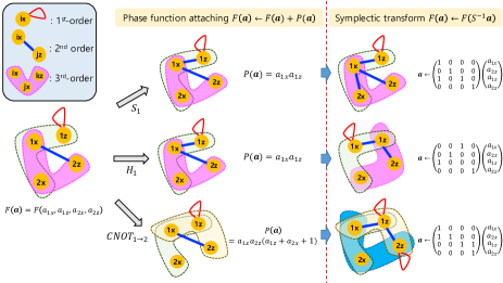
Figure 1: Hypergraph representation of frame changing. For example, the initial frame $F(\mathbf{a})=a_{1z}+a_{1x}a_{2z}+a_{1x}a_{2x}a_{2z}+a_{1x}a_{1z}a_{2x}$ transforms to $F^{\prime}(\mathbf{a})=a_{1z}+a_{1x}a_{1z}+a_{1x}a_{2x}+a_{1x}a_{2z}+a_{1x}a_{2x}a_{2z}+a_{1x}a_{1z}a_{2x}$ after the phase gate on the first qubit $S_{1}$ (the upper-most graphs). Vertices connected by hyperedges comprise variables forming a single term in frame. $A\leftarrow B$ denotes that $A$ is replaced by $B$.

Figure 1 presents $S(\mathbf{a})$ and $P(\mathbf{a})$ for a set of quantum gates $\{H,S,CNOT\}$, from which any Clifford circuit can be generated. We note that the phase functions for these gates have at most three terms of phase space coordinates $a_{i\alpha}$ for $i=1,\cdots,n$, and $\alpha=x,z$. Hence, the frame function that does not generate negativity under Clifford gates can be expressed as a third-order Boolean function, $F(\mathbf{a})=\sum_{i,j,k=1}^{n}\sum_{\alpha,\beta,\gamma=x,z}A_{ijk}^{\alpha\beta\gamma}a_{i\alpha}a_{j\beta}a_{k\gamma}+\sum_{i,j=1}^{n}\sum_{\alpha,\beta=x,z}B_{ij}^{\alpha\beta}a_{i\alpha}a_{j\beta}+\sum_{i=1}^{n}\sum_{\alpha=x,z}C_{i}^{\alpha}a_{i\alpha}\leavevmode\nobreak\ \leavevmode\nobreak\ \pmod{2}$ with binary coefficients $A_{ijk}^{\alpha\beta\gamma},B_{ij}^{\alpha\beta},C_{i}^{\alpha}\in\{0,1\}$. While storing the frame function requires $\mathcal{O}(n^{3})$ memory cost, it can be more compactly represented by using a hypergraph with vertices $V=\{v_{1x},\cdots,v_{nx},v_{1z},\cdots,v_{nz}\}$ corresponding to the phase space coordinates and hyperedges $E=\{\{v_{i\alpha},v_{j\beta},v_{k\gamma}\}\}_{A_{ijk}^{\alpha\beta\gamma}=1}\bigcup\{\{v_{i\alpha},v_{j\beta}\}\}_{B_{ij}^{\alpha\beta}=1}\bigcup\{\{v_{i\alpha}\}\}_{C_{i}^{\alpha}=1}$ corresponding to non-vanishing coefficients. Figure 1 describes the hypergraph representation of the phase function and its transformation under the Clifford gates. In this case, frame changing under a single two-qubit Clifford gate takes $\mathcal{O}(n^{2})$-time (see Supplemental Material (SM) [29] for more details).

Classical simulation of Clifford circuits with non-stabilizer inputs.— We now provide our main result on the classical simulation of non-adaptive Clifford circuits using the framed Wigner function. We establish sufficient conditions for classically efficient weak simulation that samples the measurement outcomes whose statistics are indistinguishable from those of the quantum circuit [5].

Theorem 1.

Suppose an $n$-qubit quantum circuit composed of an input state $\rho$, a Clifford unitary $U$, and measurements on the computational basis. If the circuit satisfies the following conditions:

1. Initial phase points of $\rho$ is positively represented under $F$ and can be efficiently sampled,

2. The final frame $F^{\prime}$ after applying $U$ only has first-order terms in $z$-coordinates, i.e., $F^{\prime}({\bf 0}_{x},\mathbf{a}_{z})=\mathbf{k}\cdot\mathbf{a}_{z}$ for some $\mathbf{k}\in\mathbb{Z}^{n}_{2}$,

then a classical algorithm can simulate it with $\mathcal{O}(n^{2})$-time complexity.

We sketch the proof of Theorem 1, while more details can be found in SM [29]. We first note that the overlap between $\ket{\mathbf{y}}=\ket{y_{1}y_{2}\cdots y_{n}}$ in the computational basis and the final phase space operator $UA^{F}(\mathbf{u})U^{\dagger}=A^{F^{\prime}}(\mathbf{u}^{\prime})$ in Eq. (5) with $\mathbf{u}^{\prime}=S(\mathbf{u})$ can be written as

$$\bra{\mathbf{y}}A^{F^{\prime}}(\mathbf{u}^{\prime})\ket{\mathbf{y}} =\frac{1}{2^{n}}\sum_{\mathbf{a}\in\mathbb{Z}_{2}^{2n}}(-1)^{[\mathbf{u}^{\prime},\mathbf{a}]+F^{\prime}(\mathbf{a})}\bra{\mathbf{y}}T_{\mathbf{a}}\ket{\mathbf{y}}$$ (6)

$$=\frac{1}{2^{n}}\sum_{\mathbf{a}_{z}\in\mathbb{Z}^{n}_{2}}(-1)^{(\mathbf{u}^{\prime}_{x}+\mathbf{y})\cdot\mathbf{a}_{z}+F^{\prime}(\mathbf{0}_{x},\mathbf{a}_{z})}$$

$$=\frac{1}{2^{n}}\sum_{\mathbf{a}_{z}\in\mathbb{Z}^{n}_{2}}(-1)^{(\mathbf{u}^{\prime}_{x}+\mathbf{y}+\mathbf{k})\cdot\mathbf{a}_{z}}$$

$$=\delta_{\mathbf{y},\mathbf{u}^{\prime}_{x}+\mathbf{k}},$$

where we used the fact $\bra{\mathbf{y}}T_{\mathbf{a}}\ket{\mathbf{y}}=(-1)^{\mathbf{y}\cdot\mathbf{a}_{z}}\delta_{\mathbf{a}_{x},\mathbf{0}_{x}}$ and the condition $F^{\prime}(\mathbf{0}_{x},\mathbf{a}_{z})=\mathbf{k}\cdot\mathbf{a}$. Consequently, the outcomes of the quantum circuit with probabilities,

$$p(\mathbf{y}) \equiv\Tr[U\rho U^{\dagger}\ket{\mathbf{y}}\bra{\mathbf{y}}]$$ (7)

$$=\sum_{\mathbf{u}\in\mathbb{Z}_{2}^{2n}}W^{F}_{\rho}(\mathbf{u})\bra{\mathbf{y}}UA^{F}(\mathbf{u})U^{\dagger}\ket{\mathbf{y}}$$

$$=\sum_{\mathbf{u}\in\mathbb{Z}_{2}^{2n}}W^{F}_{\rho}(\mathbf{u})\delta_{\mathbf{y},\mathbf{u}^{\prime}_{x}+\mathbf{k}},$$

can be sampled by the following procedure:

1. Sample a phase space point $\mathbf{u}\in\mathbb{Z}_{2}^{2n}$ from $W^{F}_{\rho}(\mathbf{u})$ with the initial frame $F$.

2. Update $\mathbf{u}$ to $\mathbf{u}^{\prime}\equiv S(\mathbf{u})$.

3. From $\mathbf{u}^{\prime}$ and the frame function $F^{\prime}(\mathbf{0}_{x},\mathbf{a}_{z})=\mathbf{k}\cdot\mathbf{a}_{z}$, output $\mathbf{y}=\mathbf{u}^{\prime}_{z}+\mathbf{k}$.

As the phase functions of the Clifford gates have up to third-order terms, satisfying the condition $F^{\prime}(\mathbf{0}_{x},\mathbf{a}_{z})=\mathbf{k}\cdot\mathbf{a}_{z}$ might be considered challenging even with stabilizer inputs. Nevertheless, we show that any non-adaptive Clifford circuit can be efficiently simulated by the framed Wigner function method [29].

Corollary 1.

Any non-adaptive Clifford circuit with stabilizer inputs can be efficiently transformed into a circuit satisfying the conditions in Theorem 1 so that it can be classically simulated in $\mathrm{poly}(n)$-time.

Figure 2: The process of the greedy algorithm for vertex cover problem. For each step, a vertex with the largest number of hyperedges is removed. By removing vertices $v_{5z},v_{1z},v_{6z}$ at each step (indicated by inverted color), the resulting frame only contains a linear term $a_{3z}$. Red dashed lines are sections at which the frame graph has the above form.

For non-stabilizer inputs, however, it is uncommon to find a case to meet the conditions in Theorem 1. This can be understood in the same line as the hardness of classically simulating non-adaptive Clifford circuits with non-stabilizer inputs [5]. Although simulating all the outcome qubits remains difficult, our formalism offers an efficient classical simulation of some marginal outcomes, which goes beyond the Gottesman-Knill tableau method. This can be done by observing that after tracing out the $j$th qubit, the phase space operator of the remaining qubits is given by substituting $(a_{jx},a_{jz})=(0,0)$ to the final frame function $F^{\prime}$, thus removing all the terms containing $a_{jx}$ or $a_{jz}$. Hence, after tracing out a sufficiently large number of qubits, one can reduce the frame function to be linear for the remaining qubits, which can be classically simulated efficiently. More precisely, such a problem can be translated to the vertex cover problem for a hypergraph [27] to find the minimum number of vertices to cover all the second and third-order hyperedges. Such a problem is known to be an NP-hard problem [30], but one can take a sub-optimal algorithm, for example a greedy algorithm [27] running in poly-time. A schematic procedure to find a linear frame function by tracing out some qubits is described in Fig. 2.

Random circuits with log-depth.— We apply the protocol to two different types of random $n$-qubit log-depth Clifford circuits with 1D-neighboring and arbitrary long-range interactions (completely connected) between two qubits [31], where gate count is $L=\alpha n\ln(n)$. A brief explanation of these two architectures is shown in Ref. [29]. In both cases, we obtain the final frame $F^{\prime}(\mathbf{a})$ starting from $F({\mathbf{a}})=0$ and use the greedy algorithm to find efficiently simulatable marginal qubits. Figure 3(a,c) shows that our simulation method successfully samples the measurement outcomes.

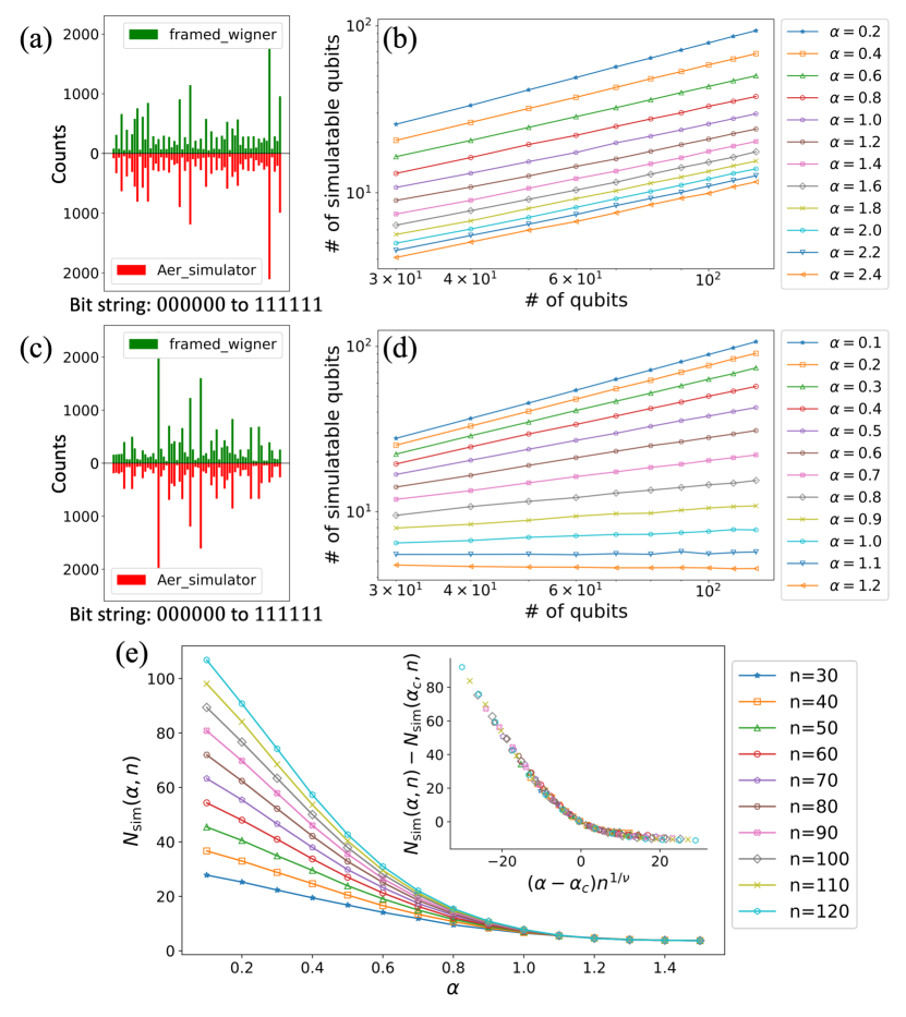
Figure 3: (a), (c): Comparison between sampling results using the framed Wigner function and Qiskit Aer simulator for a randomly chosen $10$-qubit log-depth Clifford circuit with (a) 1D-neighboring and (c) completely connected architecture. For both cases, non-stabilizer input state $\ket{A}\bra{A}^{\otimes 10}$ is taken, and $6$ marginal qubits are selected after solving the vertex cover problem. The $y$-axis shows the number of counts of binary string that simulators sampled by taking total $20000$ samples. (b), (d): The averaged number of simulatable qubits ($N_{\rm sim}$) by increasing the gate count $L=\alpha(n\ln n)$ of random Clifford circuits with (b) 1D-neighboring and (d) completely connected architectures. 1000 random circuits are sampled for each point. (e) Scaling behavior of $N_{\rm sim}$ by increasing $\alpha$ and data collapse after finite-size scaling.

Figure 3(b) shows that for 1D architecture, the average number of classically simulatable qubits ($N_{\rm sim}$) increases linearly by the circuit size. Such a circuit can be fully and classically simulated [32] by using the tensor network, while its time complexity exponentially grows with the circuit depth as $e^{\mathcal{O}(\alpha\ln n)}\geq n^{\mathcal{O}(\alpha)}$. Although our simulation method is limited to selected marginal qubits, we show that [29] the time complexity to simulate these marginal qubits is upper bounded by $\mathcal{O}(n(\ln(n))^{4})+n^{2}\ln(n))$, including frame changing and greedy algorithm, which can be faster than the tensor network method when $\alpha$ becomes larger. From numerical simulation [29], we observe remarkable improvement in the computation time of the marginal sampling when using our method compared to the matrix product state simulator of the IBM Qiskit.

On the other hand, for the completely connected architecture, we observe a sharp transition of $N_{\rm sim}$ depending on the parameter $\alpha$ that determines the total gate count. For $\alpha\leq\alpha_{c}$, $N_{\rm sim}$ scales quasi-linearly by increasing the number of qubits. In contrast, if the gate count exceeds a certain value $\alpha\geq\alpha_{c}$, we observe the sub-linear scaling of the $N_{\rm sim}$ (see Fig. 3(d)). From the finite-size scaling analysis by taking a general scaling form $N_{\rm sim}(\alpha,n)-N_{\rm sim}(\alpha_{c},n)=f((\alpha-\alpha_{c})n^{1/\nu})$ [33], we numerically estimate the critical value $\alpha_{c}\approx 0.81$ and $\nu\approx 1.28$ (see Fig. 3(e)). While the critical point closely aligns with the point $\alpha=5/6$ that governs the anti-concentration properties of the completely connected random circuit [31], we defer the exploration of the direct relationship between these two critical values to future research.

Born probability estimation.— Theorem 1 provides a strict condition on an exact and efficient classical sampling of Clifford circuits from the framed Wigner function. We further show that the Born probability of a particular outcome $p(\mathbf{y})$ can be estimated using the same framework with a less restrictive condition. We recall from Eqs. (6) and (7) that

$$p(\mathbf{y})=\frac{1}{2^{n}}\sum_{\mathbf{u}\in\mathbb{Z}_{2}^{2n}}\sum_{\mathbf{a}_{z}\in\mathbb{Z}^{n}_{2}}W^{F}_{\rho}(\mathbf{u})(-1)^{(\mathbf{u}^{\prime}_{x}+\mathbf{y})\cdot\mathbf{a}_{z}+F^{\prime}(\mathbf{0}_{x},\mathbf{a}_{z})}.$$ (8)

A naïve way to estimate $p(\mathbf{y})$ within additive error is sampling a binary string $\mathbf{a}_{z}\in\mathbb{Z}^{n}_{2}$ from the uniform distribution and taking an unbiased estimator $\hat{p}_{\mathbf{a}_{z}}(\mathbf{y})=\sum_{\mathbf{u}}W^{F}_{\rho}(\mathbf{u})(-1)^{(\mathbf{u}^{\prime}_{x}+\mathbf{y})\cdot\mathbf{a}_{z}+F^{\prime}(\mathbf{0}_{x},\mathbf{a}_{z})}$, satisfying $\mathbb{E}_{\mathbf{a}_{z}}[\hat{p}_{\mathbf{a}_{z}}(\mathbf{y})]=p(\mathbf{y})$ by averaging over $\mathbf{a}_{z}$. This estimator can be efficiently calculated whenever $W^{F}_{\rho}(\mathbf{u})$ has a product form, regardless of its positiveness. We note that this method is equivalent to randomly sampling the Pauli operators studied in Ref. [34] and has the estimation variance ${\rm Var}_{\rm Pauli}(\mathbf{y})\equiv\mathbb{E}_{\mathbf{a}_{z}}[|\hat{p}_{\mathbf{a}_{z}}(\mathbf{y})-p(\mathbf{y})|^{2}]=Z_{U,\rho}-p(\mathbf{y})^{2}$ [29], where $Z_{U,\rho}\equiv\sum_{\mathbf{y}\in\mathbb{Z}^{n}_{2}}p(\mathbf{y})^{2}$ is the collision probability [35, 31]. Consequently, the average estimation variance over all outcomes $\mathbf{y}$ becomes $\Delta_{\rm Pauli}\equiv 1/2^{n}\sum_{\mathbf{y}\in\mathbb{Z}_{2}^{n}}{\rm Var}_{\rm Pauli}(\mathbf{y})=(1-1/2^{n})Z_{U,\rho}$.

We propose an alternative way that genuinely utilizes the probabilistic nature of the Wigner function [29]. When the circuit meets the first condition of Theorem 1, one can sample $\mathbf{u}$ efficiently from $W^{F}_{\rho}(\mathbf{u})$ and take the estimator $\hat{p}_{\mathbf{u}}(\mathbf{y})=\frac{1}{2^{n}}\sum_{\mathbf{a}_{z}\in\mathbb{Z}^{n}_{2}}(-1)^{(\mathbf{u}^{\prime}_{x}+\mathbf{y})\cdot\mathbf{a}_{z}+F^{\prime}(\mathbf{0}_{x},\mathbf{a}_{z})}$, satisfying $\mathbb{E}_{\mathbf{u}}[\hat{p}_{\mathbf{u}}(\mathbf{y})]=p(\mathbf{y})$. The average estimation variance is $\Delta_{\rm Wig}\equiv 1/2^{n}\sum_{\mathbf{y}\in\mathbb{Z}_{2}^{n}}{\rm Var}_{\rm Wig}(\mathbf{y})=(1-Z_{U,\rho})/2^{n}$ for any quantum circuits. This implies that $\Delta_{\rm Wig}\leq\Delta_{\rm Pauli}$ as $Z_{U,\rho}\geq 2^{-n}$.

On the other hand, this method is efficient only if the final frame $F^{\prime}(\mathbf{0}_{x},\mathbf{a}_{z})$ does not contain third-order terms. Otherwise, evaluating the exponential sum in $\hat{p}_{\mathbf{u}}(\mathbf{y})$ becomes an #P-hard problem [36]. Nonetheless, similarly to the weak simulation scheme, tracing out $(n-k)$ qubits until the final frame does not contain third-order terms yields an efficient estimation of $k$-marginal outcome probability. As second-order terms in the final frame function are allowed, the number of efficiently estimable marginal outcomes is generally larger than that for efficient weak simulation. In this case, we show that the average estimation variance of $k$-marginal outcome probability $p(\mathbf{y}^{\prime})$ becomes $\Delta_{\rm Wig}^{(k)}\equiv 1/2^{k}\sum_{\mathbf{y}^{\prime}\in\mathbb{Z}_{2}^{k}}{\rm Var}_{\rm Wig}(\mathbf{y}^{\prime})=(1-Z^{(k)}_{U,\rho})/2^{k}$, while the Pauli sampling method yields $\Delta_{\rm Pauli}^{(k)}\equiv 1/2^{k}\sum_{\mathbf{y}^{\prime}\in\mathbb{Z}_{2}^{k}}{\rm Var}_{\rm Pauli}(\mathbf{y}^{\prime})=(1-1/2^{k})Z_{U,\rho}^{(k)}$ with $Z_{U,\rho}^{(k)}=\sum_{\mathbf{y}^{\prime}\in\mathbb{Z}_{2}^{k}}p(\mathbf{y}^{\prime})^{2}\geq 2^{-k}$. Therefore, if $Z_{U,\rho}^{(k)}$ is sufficiently larger than $2^{-k}$, our methods show an improvement of the estimation time for a large fraction of marginal strings $\mathbf{y}^{\prime}$.

Remarks.— We have introduced the framed Wigner function and formulated the frame-changing rules that do not induce negativity under any Clifford gates. Based on our formalism, we have developed a classical simulation algorithm for a non-adaptive Clifford circuit with non-stabilizer inputs and established sufficient conditions to execute the algorithm. Also, we construct a systematic protocol to find marginal outcome measurements that can be efficiently classically simulated by solving the vertex cover problem. As examples, we have explored $\log$-depth Clifford circuits and observed that the number of simulatable qubits behaves differently between locally and completely connected circuits.

Our approach of introducing a family of frame functions paves the way for understanding the connection between qubit Clifford operations and the non-negativity in the Wigner function. At the same time, it leaves potential extensions and further exploration. A crucial question would be asking whether the proposed methods based on the framed Wigner function can be further extended to classically simulate quantum circuits with non-Clifford gates.

I Supplemental Material

II Section $\mathbf{I}$: Generalized representation of the framed Wigner function

Throughout this paper, we denote $n$ as the number of qubits in circuits. In the main text, we represented a quantum state $\rho$ as a fixed frame function $F$. However, we do not need to stick to a fixed frame when we define the Wigner function. We say a quantum state $\rho$ is p-th ordered positively represented under $\mathcal{F}$ if and only if there exists a set of up to $p$-th ordered Boolean functions (p-frame set) $\mathcal{F}$ and non-negative distribution $W^{F}_{\rho}(\mathbf{u})\;(F\in\mathcal{F},\sum_{\mathbf{u},F}W^{F}(\mathbf{u})=1)$ such that

$$\rho=\sum_{\mathbf{u}\in\mathbb{Z}^{2n}_{2},F\in\mathcal{F}}W^{F}_{\rho}(\mathbf{u})A^{F}(\mathbf{u}).$$ (9)

From now on, we assume that the maximal order is lower than or equal to $3$.

We note that a single qubit state can be expressed as a convex sum of eight phase point operators, half of them are from zero frame ($F=0$), and the others are from dual frame, $F=a_{1x}a_{1z}$ [20]. Hence, if $\rho$ is a product state, it is second-ordered positively represented under 2-frame set $\mathcal{F}\equiv\left\{\mathbf{b}\cdot(a_{1x}a_{1z},a_{2x}a_{2z},\ldots,a_{nx}a_{nz})|\mathbf{b}\in\mathbb{Z}^{n}_{2}\right\}$. More precisely, for $\rho=\bigotimes_{i=1}^{n}\rho_{i}$, we express each $\rho_{i}$ as

$$\rho_{i}=\sum_{\mathbf{u}_{i}\in\mathbb{Z}^{2}_{2}}\left(W^{0}_{\rho_{i}}(\mathbf{u}_{i})A^{0}(\mathbf{u}_{i})+W^{a_{ix}a_{iz}}_{\rho_{i}}(\mathbf{u}_{i})A^{a_{ix}a_{iz}}(\mathbf{u}_{i})\right),$$ (10)

where $\mathbf{u}_{i}\equiv(u_{ix},u_{iz})$. We note that these two functions, $W^{0}_{\rho_{i}}(\mathbf{u}_{i})$ and $W^{a_{ix}a_{iz}}_{\rho_{i}}(\mathbf{u}_{i})$ cannot be obtained by inversion in Eq. (1) of the main text because we now have eight phase point operators and these are not Hilbert-Schmidt orthogonal to each other. However, we can still efficiently find these two functions because the convex polytope by 8-phase point operators as extreme points contains the Bloch sphere and its dimension is constant. Hence solving the constant-sized system of linear equations is enough to find those functions. Next, we can express $\rho$ as follows,

$$\rho =\bigotimes_{i=1}^{n}\rho_{i}=\sum_{\mathbf{b}\in\mathbb{Z}^{n}_{2}}\sum_{\mathbf{u}\in\mathbb{Z}^{2n}_{2}}\left(\prod_{i=1}^{n}W^{b_{i}a_{ix}a_{iz}}_{\rho_{i}}(\mathbf{u}_{i})\bigotimes_{i=1}^{n}A^{b_{i}a_{ix}a_{iz}}(\mathbf{u}_{i})\right),$$ (11)

where $\mathbf{u}=\bigoplus_{i}^{n}(\mathbf{u}_{i})$. We can easily note from the definition that $\bigotimes_{i=1}^{n}A^{b_{i}a_{ix}a_{iz}}(\mathbf{u}_{i})$ is an $n$-qubit phase point operators with a frame polynomial $F=\mathbf{b}\cdot(a_{1x}a_{1z},a_{2x}a_{2z},\ldots,a_{nx}a_{nz})$. Hence, we can rewrite Eq.(11) as

$$\rho=\sum_{F\in\mathcal{F}}\sum_{\mathbf{u}\in\mathbb{Z}^{2n}_{2}}\left(\prod_{i=1}^{n}W^{b_{i}a_{ix}a_{iz}}_{\rho_{i}}(\mathbf{u}_{i})A^{F}(\mathbf{u})\right).$$ (12)

Therefore, the desired Wigner function is

$$W^{F}_{\rho}(\mathbf{u})=\prod_{i=1}^{n}W^{b_{i}a_{ix}a_{iz}}_{i}(\mathbf{u}_{i}).$$ (13)

We note that this may not be a unique expression, but it does not matter if we are only considering the sampling phase point from $\rho$ within $\mathcal{O}(n)$-time. The non-negative function $W^{F}_{\rho}$ is a probability distribution with random variables of not only $\mathbf{u}$ but also $F$, so that we can sample both $\mathbf{u}$ and $F$ from $W^{F}_{\rho}(\mathbf{u})$. Since the Wigner function has a product form and for each $i\in[n]$, we sample $\mathbf{u}_{i}$ and $b_{i}$ from $W^{b_{i}a_{ix}a_{iz}}_{i}(\mathbf{u}_{i})$. The resulting sampling outcome then becomes $\mathbf{u}=\bigoplus_{i}^{n}(\mathbf{u}_{i})$ and $F=\mathbf{b}\cdot(a_{1x}a_{1z},a_{2x}a_{2z},\ldots,a_{nx}a_{nz})$. After then, we can follow the same procedure described in the main text for simulating the quantum circuits. However, conditions for efficient weak simulation become more restricted because we have multiple final frames, so multiple conditions of the final frame. We will discuss this in detail in Theorem 2.

III Section $\mathbf{II}$: Frame changing and time-complexity

As we discussed in the main text, the frame can be changed when applying a Clifford unitary $U$. This takes $\rho$ to

$$U\rho U^{\dagger} =\frac{1}{2^{n}}\sum_{\mathbf{u},F\in\mathcal{F},\mathbf{a}}W^{F}_{\rho}(\mathbf{u})\left(-1\right)^{[\mathbf{u},\mathbf{a}]+F(\mathbf{a})}UT_{\mathbf{a}}U^{\dagger}$$

$$=\frac{1}{2^{n}}\sum_{\mathbf{u},F\in\mathcal{F},\mathbf{a}}W^{F}_{\rho}(\mathbf{u})\left(-1\right)^{[\mathbf{u},\mathbf{a}]+F(\mathbf{a})+P(\mathbf{a})}T_{S(\mathbf{a})}$$

$$=\frac{1}{2^{n}}\sum_{\mathbf{u},F\in\mathcal{F},\mathbf{a}}W^{F}_{\rho}(\mathbf{u})\left(-1\right)^{[S(\mathbf{u}),\mathbf{a}]+F(S^{-1}(\mathbf{a}))+P(S^{-1}(\mathbf{a}))}T_{\mathbf{a}}$$

$$=\frac{1}{2^{n}}\sum_{\mathbf{u},F\in\mathcal{F},\mathbf{a}}W^{F}_{\rho}(S^{-1}(\mathbf{u}))\left(-1\right)^{[\mathbf{u},\mathbf{a}]+F(S^{-1}(\mathbf{a}))+P(S^{-1}(\mathbf{a}))}T_{\mathbf{a}},$$ (14)

where

$$UT_{\mathbf{a}}U^{\dagger}=(-1)^{P(\mathbf{a})}T_{S(\mathbf{a})}.$$ (15)

Clifford gate	$S$	$P(\mathbf{a})$
$CNOT_{i\rightarrow j}$-gate	$\begin{subarray}{c}a_{iz}\longleftarrow a_{iz}+a_{jz}\\ a_{jx}\longleftarrow a_{ix}+a_{jx}\end{subarray}$	$a_{jz}a_{ix}(a_{iz}+a_{jx}+1)$
$CZ_{ij}$-gate	$\begin{subarray}{c}a_{iz}\longleftarrow a_{iz}+a_{jx}\\ a_{jz}\longleftarrow a_{ix}+a_{jz}\end{subarray}$	$a_{jx}a_{ix}(a_{iz}+a_{jz})$
$H_{i}$-gate	$\begin{subarray}{c}a_{ix}\longleftarrow a_{iz}\\ a_{iz}\longleftarrow a_{ix}\end{subarray}$	$a_{iz}a_{ix}$
$S_{i}$-gate	$a_{iz}\longleftarrow a_{ix}+a_{iz}$	$a_{iz}a_{ix}$

Table 1: A table that shows the symplectic transformation of each Clifford basis operator ($S$) and corresponding phase function ($P(\mathbf{a})$). $A\leftarrow B$ means $A$ is transformed to $B$.

Table 1 shows symplectic matrices $S$ and phase functions $P(\mathbf{a})$ for each Clifford basis. From this, we can easily obtain symplectic matrices of all Clifford circuits (including Pauli operations) and the resulting final frame after the operations.

Suppose that a given $d$-depth Clifford circuit consists of $poly(n)$-number of 2-qubit Clifford gate, and the initial frame is of $3$rd order. With $\mathcal{O}(1)$-complexity we can find the symplectic matrix and phase function of a 2-qubit gate. Changing the frame under the gate takes $\mathcal{O}(n^{2})$-time because we only consider monomials having variables with an index that we will transform, and the maximal number of those monomials is at most $\mathcal{O}(n^{2})$. Hence frame changing after a single depth operation takes $\mathcal{O}(n^{3})$-time, and total changing time takes $\mathcal{O}(dn^{3})$-time. Also, this argument implies that during the early time of frame changing, the number of total monomials in the frame polynomial itself is low, so the frame changes much faster. Throughout the change, we need at most $\frac{(2n+1)^{3}}{6}$-memory.

Furthermore, if a circuit has shallow depth, we can reduce the order of changing time.

Proposition 1.

Suppose we start from the frame $F=\sum_{i=1}^{n}b_{i}a_{ix}a_{iz}$, where $\forall i,\;b_{i}\in\left\{0,1\right\}$.

(i) If the given circuit has 1D architecture and depth $d$, then obtaining a resulted frame polynomial takes at most $\min{\left\{\mathcal{O}(dn^{3}),\mathcal{O}(d^{4}n+dn^{2})\right\}}$. For a complete graph architecture with depth $d$, it takes at most $\min{\left\{\mathcal{O}(dn^{3}),\mathcal{O}(8^{d}\cdot dn+dn^{2})\right\}}$. To do so, we need $\mathcal{O}(dn^{2}+n^{3})$-memory.
(ii) There exists a method to uniformly randomly choose a Clifford circuit such that obtaining resulted frame takes at most $\mathcal{O}(n^{4})$.

Proof.

(i) Following the previous arguments, the algorithm with $\mathcal{O}(dn^{3})$-complexity can be easily obtained. Next, let us assume that for each stage $1\leq i\leq d$, we act the Clifford operation $U_{i}\equiv\bigotimes_{j=1}^{k_{i}}U_{ij}$ where $k_{i}\in\mathbb{N},k_{i}\leq\lfloor\frac{n}{2}\rfloor$ and $U_{ij}$ is 2-qubit Clifford operation. We can obtain the symplectic matrix $S_{i}$ and phase function $P_{i}$ in $\mathcal{O}(n)$-time because, for each $j$, the symplectic transform of 2-qubit operation does not affect other qubit pairs. Now, from the arguments in Eq. (14) and Eq. (15), we easily note that resulted symplectic transform $S$ and phase function $P$ is,

$$S =S_{d}S_{d-1}\ldots S_{1},$$

$$P =P_{1}(\mathbf{a})+P_{2}(S_{1}(\mathbf{a}))+P_{3}(S_{2}(S_{1}(\mathbf{a})))+\cdots+P_{d}(S_{d-1}(S_{d-2}\cdots(S_{2}(S_{1}(\mathbf{a})))\cdots)).$$ (16)

Hence the resulting frame polynomial $K$ becomes,

$$K=F(S^{-1}(\mathbf{a}))+P(S^{-1}(\mathbf{a})) =P_{1}(S^{-1}_{1}(S^{-1}_{2}\cdots(S^{-1}_{d-1}(S^{-1}_{d}(\mathbf{a})))\cdots))+P_{2}(S^{-1}_{2}(S^{-1}_{3}\cdots(S^{-1}_{d-1}(S^{-1}_{d}(\mathbf{a})))\cdots))$$

$$+\cdots+P_{d-1}(S^{-1}_{d-1}((S^{-1}_{d}(\mathbf{a}))))+P_{d}(S^{-1}_{d}(\mathbf{a}))+F(S^{-1}_{1}(S^{-1}_{2}\cdots(S^{-1}_{d-1}(S^{-1}_{d}(\mathbf{a})))\cdots)).$$ (17)

Each $S_{i}$ can be expressed as a tensor product $\bigotimes_{j=1}^{k_{i}}S_{ij}$ of $4\times 4$ matrices, which leads to $S^{-1}_{i}=\bigotimes_{j=1}^{k_{i}}S^{-1}_{ij}$. The time complexity to multiply arbitrary $2n\times 2n$ matrix and $A\otimes I_{1}\otimes\cdots\otimes I_{k_{i}-1}$, where A is a $4\times 4$ matrix and $I_{1},\ldots,I_{k_{i}-1}$ are $4\times 4$ identities, is $\mathcal{O}(n)$. Therefore, starting from $S^{-1}_{d}$ and calculating up to $S^{-1}_{1}(S^{-1}_{2}\cdots(S^{-1}_{d-1}(S^{-1}_{d}(\mathbf{a})))\cdots)$ takes $\mathcal{O}(dn^{2})$-time. By multiplying each $S^{-1}_{i}$’s, we record all $d-1$ output matrices. To do so, we need $\mathcal{O}(dn^{2})$-memory.

Now, we prepare $\mathcal{O}(dn^{2}+n^{3})$-memory (say $M$) to record each coefficient of single terms in the frame. We first set all coefficients to zero. We will put $1$’s properly such that the resulting matrix be a desired final frame.

For the 1D case, for $m\in[n]$, we easily note that $S^{-1}(\mathbf{a})_{mx(or\;mz)}$ does not have variable $a_{qx(or\;qz)}$ where $|m-q|\;(mod\;n)\geq d$. If $S^{-1}(\mathbf{a})_{mx(or\;mz)}$ has such variables, two-qubit operation blocks must have propagated from q-th qubit to m-th qubit, but this is not the case for the 1D case. Since each $P_{i}$ is at most of 3rd-order and has at most $\mathcal{O}(n)$ monomials, expanding $P_{i}(S^{-1}_{i}(S^{-1}_{i+1}\cdots(S^{-1}_{2}(S^{-1}_{1}(\mathbf{a})))\cdots))$ takes at most $\mathcal{O}((2d)^{3}n)$-time. Also, during the expansion, for each obtained single term, we must put $1$ to the corresponding location of $M$. If $1$ is already located, then we flip it to $0$. We repeat these steps for $d$ times hence total time is at most $\mathcal{O}(d^{4}n)$. Also, in the same manner, adding $F(S^{-1}_{1}(S^{-1}_{2}\cdots(S^{-1}_{d-1}(S^{-1}_{d}(\mathbf{a})))\cdots))$ takes $\mathcal{O}((2d)^{3}n)$-time.

For a complete graph case, the problem becomes more complicated. Each Clifford gate may entangle two qubits far from each other and then each qubit can be further affected by different long-ranged Clifford gates. As a results, $S^{-1}(\mathbf{a})_{mx(or\;mz)}$ have the number of variable $a_{qx(or\;qz)}$ at most $2^{d+1}$, so expanding $P_{i}(S^{-1}_{i}(S^{-1}_{i+1}\cdots(S^{-1}_{2}(S^{-1}_{1}(\mathbf{a})))\cdots))$ takes at most $\mathcal{O}(2^{3d+3}n)$-time. Then we encode $1$ to $M$ in the same way with 1D-case. This completes the proof of (i).

(ii) From Ref. [37], we can efficiently sample random Clifford operation in $\mathcal{O}(n^{2})$-time. This form always has the layers $F^{\prime}-S-H-F$, where $H$ is a layer of Hadamard gates, $S$ is a layer of SWAP gates (hence of CNOT gates), and $F,F^{\prime}$ are CNOT-CZ-S-Pauli layered circuits. CNOT circuit can be decomposed as Clifford bases with depth at most $\mathcal{O}(\frac{n}{\log(n)})$ with at most $\mathcal{O}(n^{3})$-time [28, 38]. Also, the depth of the CZ-layer can be upper bounded by $\mathcal{O}(n)$, with $\mathcal{O}(n^{3})$-time [39]. Therefore randomly chosen Clifford circuits can be decomposed to have a depth at most $\mathcal{O}(n)$ (in long-range form). Hence the total time complexity of frame changing is at most $\mathcal{O}(n^{4})$. ∎

Proposition 1 states that for the complete graph with $\alpha\log(n)$-depth or 1D with $n^{\alpha}$-depth where $\alpha<\frac{2}{3}$, we can find another changing algorithm with a reduced order of $n$. Since the above frame changing is only given by rotations of phase and the argument of the Pauli operator, the application of those algorithms is wider than the scope of the main text.

IV Section III: Basic notation of graph theory

Here, we introduce a formal definition of hypergraph and the vertex cover problem.

Definition 1 (Hypergraph).

(i)Let $V$ be a non-empty set. We say a tuple $G(V,E)$ is a hypergraph if and only if $E$ is a set of subsets $e\in V$ of $V$. We call each element in $E$ an edge. From now, we always assume $\forall e\in E,|e|>1$.

Let $G(V,E)$ be a hypergraph.

(ii)If all elements of $E$ have $(k\in\mathbb{N})$-number of elements in $V$, then we call $G(V,E)$ as a $k$-uniform hypergraph or simply a k-graph. Also, a 2-graph is just called a graph.

Definition 2.

Let $G(V,E)$ be a hypergraph.

i) $V^{\prime}\subset V$ is a vertex cover if all edges in $E$ contain some elements in $V^{\prime}$. $A\subset V$ is the minimal vertex cover if every vertex cover $V^{\prime}\subset V$ satisfies $|V^{\prime}|\geq|A|$.

ii) $S^{\prime}\subset V$ is an independent set if any two elements in $S^{\prime}$ are not contained in same edge in $E$. $B\subset V$ is the maximal independent set if every independent set $S^{\prime}\subset V$ satisfies $|S^{\prime}|\leq|B|$.

iii) Let $A$ be a minimal vertex cover of $G$ and $B$ be a maximal independent set in $G$. Then we denote $\nu(G)\equiv|A|$ and $\triangle(G)\equiv|B|$. We note that minimal(maximal resp.) vertex cover(independent set) could not be unique, but $\nu(G)$ and $\triangle(G)$ are unique.

The Vertex cover problem is to find the minimum vertex cover of a given hypergraph. Now we obtain one result.

Corollary 2.

For any hypergraph $G(V,E)$, $\nu(G)+\triangle(G)\leq|V|$.

Proof.

Consider a maximal independent set $S\subset V\;(|S|=\triangle(G))$ and suppose $|V\backslash S|=|V|-\triangle(G)<\nu(G)$. Then $V\backslash S$ must not be the vertex cover. Hence there exists $e\in E$ such that $e$ does not have any elements in $V\backslash S$. Since $e$ is non-zero, without loss of generality, say $e=\left\{v^{e}_{1},v^{e}_{2},\ldots,v^{e}_{k}\right\}\subset S\;(k\geq 2)$. Since $S$ is independent, $|e|=1$, which contradicts that $k\geq 2$. In conclusion, $|V\backslash S|=|V|-\triangle(G)\geq\nu(G)\Rightarrow\nu(G)+\triangle(G)\leq|V|$. ∎

It means that the size of the maximal independent set is upper bounded by $|V|-\nu(G)$. From the main text, we note that the independent set of the graph representation of resulting frame $F^{\prime}(\mathbf{0}_{x},\mathbf{a}_{z})$ is also a set of simulatable qubits. However, the above corollary tells that finding a minimum vertex cover and tracing out the qubits corresponding to the vertices produces a larger set of simulatable qubits than finding the maximal independence set. If the graph representation is $2$-graph (resulting frame is quadratic), then it is known that $\triangle{G}=|V|-\nu(G)$.

This is an NP-hard problem [27] but several efficient and approximative algorithms are valid [40]. These algorithms may obtain vertex covers such that the size is larger than the minimal cover but is within a reasonable scale factor. The typical example we use throughout this paper is a greedy algorithm. The detailed procedure of the algorithm is as follows. Suppose we have a hypergraph $G(V,E)$.

1. For each vertex $v\in V$ of $G$, count $d(v)$ (order of $v$), the number of edges containing $v$.

2. Take $v^{\prime}={\rm argmax}_{v\in V}\left\{d(v)\right\}$.

3. Remove $v^{\prime}$ from $G$ and also remove all edges containing $v^{\prime}$.

4. Repeat the above sequences with at most $\left|V\right|$ times until no edges are left.

From that, we obtain the following corollary.

Corollary 3.

Consider the hypergraph $G(V,E)$ and let $d(v)\;(v\in V)$ denote the number of edges containing $v$. Then we also define the order of $G$, $d(G)$ as $\max_{v\in V}(d(v))$. Then the time complexity of the greedy algorithm is $\mathcal{O}(\left|V\right|^{2}d(G))$.

Proof.

The proof is trivial from the above steps of the algorithm. ∎

V Section $\mathbf{IV}$: More details on Simulation methods

V.1 Weak simulation

In this section, we provide more details on Theorem 1 in the main text.

Theorem 2.

(i) Suppose that we have a quantum state $\rho$ as input and a non-adaptive Clifford operation $U$ and $Z$-measurements. Also, we assume that $\rho$ is $3$-rd ordered positively represented under the initial Wigner function with a frame set $\mathcal{F}$, and we can sample phase points efficiently from it. We denote a resulting frame polynomial via the Clifford circuit starting from $F$ as $F^{\prime}$. Also, we assume for all $F\in\mathcal{F}$, $I_{F}\subset[n]$ satisfies that $F^{\prime}(\mathbf{a}_{x}=\mathbf{0},\mathbf{a}_{z})\big{|}_{a_{iz}=0\;{\rm for}\;i\notin I_{F}}$ is a linear Boolean function. We then can classically simulate $\left|\bigcap_{F\in\mathcal{F}}I_{F}\right|$-number of measurements.

(ii) Let $\rho$ be positively represented under a single frame $F$, and the final frame is $F^{\prime}$. We take $I_{F}$ such that $F^{\prime}(\mathbf{a}_{x}=\mathbf{0},\mathbf{a}_{z})\big{|}_{a_{iz}=0\;{\rm for}\;i\notin I_{F}}$ is a quadratic Boolean function. Then we can simulate to obtain at least $\lfloor\frac{\left|I_{F}\right|+1}{2}\rfloor$ number of Boolean function values with the arguments of $Z$-measurement outcomes.

Proof.

We start from Eq. (14). Probability to measure $\mathbf{y}\in\mathbb{Z}^{n}_{2}$ is

$${\rm Tr}(\ket{\mathbf{y}}\bra{\mathbf{y}}U\rho U^{\dagger}) =\sum_{\mathbf{u},F\in\mathcal{F},\mathbf{a}_{z}\in\mathbb{Z}^{n}_{2}}\frac{1}{2^{n}}W^{F}_{\rho}(S^{-1}(\mathbf{u}))\left(-1\right)^{(\mathbf{u}+\mathbf{y})\cdot\mathbf{a}_{z}+F(S^{-1}(\mathbf{0}_{x},\mathbf{a}_{z}))+P(S^{-1}(\mathbf{0}_{x},\mathbf{a}_{z}))}$$

$$=\sum_{\mathbf{u},F\in\mathcal{F},\mathbf{a}_{z}\in\mathbb{Z}^{n}_{2}}\frac{1}{2^{n}}W^{F}_{\rho}(S^{-1}(\mathbf{u}))\left(-1\right)^{((\mathbf{u}+\mathbf{y})\cdot\mathbf{a}_{z}+F^{\prime}(\mathbf{0}_{x},\mathbf{a}_{z}))}.$$ (18)

Now, consider measuring a subset $\bigcap_{F\in\mathcal{F}}I_{F}$ of qubits. The probability to measure a marginal string $\mathbf{y}^{\prime}$ is,

$$p(\mathbf{y}^{\prime}) =\sum_{\mathbf{y}^{\prime\prime}}{\rm Tr}(\ket{\mathbf{y}^{\prime}\oplus\mathbf{y}^{\prime\prime}}\bra{\mathbf{y}^{\prime}\oplus\mathbf{y}^{\prime\prime}}U\rho U^{\dagger})$$

$$=\sum_{\mathbf{u},F\in\mathcal{F}}\left(\sum_{\begin{subarray}{c}\mathbf{a}_{z}\in\mathbb{Z}^{n}_{2}\\ a_{iz}=0\;{\rm for}\;i\in\left(\bigcap_{F\in\mathcal{F}}I_{F}\right)\end{subarray}}\frac{1}{2^{\left|\bigcap_{F\in\mathcal{F}}I_{F}\right|}}W^{F}_{\rho}(S^{-1}(\mathbf{u}))\left(-1\right)^{((\mathbf{u}_{x}+(\mathbf{y}^{\prime}\oplus 0)+\mathbf{k}_{F})\cdot\mathbf{a}_{z})}\right)$$

$$=\sum_{\mathbf{u},F\in\mathcal{F}}W^{F}_{\rho}(\mathbf{u})\prod_{i\in\left(\bigcap_{F\in\mathcal{F}}I_{F}\right)}\delta_{(\mathbf{y}^{\prime}\oplus 0)_{i},S(\mathbf{u})_{ix}+(\mathbf{k}_{F})_{i}},$$ (19)

for some marginal string $\mathbf{k}_{F}$. Therefore, we obtain the following simulation scheme given that the conditions in Theorem 2 for the final frame hold.

1. Sample a phase space point $\mathbf{u}\in\mathbb{Z}_{2}^{2n}$ and $F\in\mathcal{F}$ from $W^{F}_{\rho}(\mathbf{u})$.

2. Update $F$ to $F^{\prime}$

3. Update $\mathbf{u}$ to $\mathbf{u}^{\prime}\equiv S(\mathbf{u})$.

4. From $\mathbf{u}^{\prime}$ and the frame function $F^{\prime}(\mathbf{0},\mathbf{a}_{z})=\mathbf{k}_{F}\cdot\mathbf{a}_{z}$, take $\mathbf{y}=\mathbf{u}^{\prime}_{x}+\mathbf{k}$.

5. Desired outcome is a marginal string $(y_{i})_{i\in\left(\bigcap_{F\in\mathcal{F}}I_{F}\right)}$.

We already showed in Proposition 1 that the time complexity of frame changing and obtaining $S$ is up to $poly(n)$. Also, updating $\mathbf{u}$ to $\mathbf{u}^{\prime}$ is a sinple matrix multiplication which takes $\mathcal{O}(n^{2})$ time. Hence total simulation time is $poly(n)$. However, if $\rho$ is positively represented under a single frame function, then at step 1 we only choose that frame from the Wigner function. In this case, we only choose and change the frame only once, and for the next sampling, we only sample and change $\mathbf{u}$.

(ii) We first assume that $F^{\prime}(\mathbf{a}_{x}=\mathbf{0},a_{z})\big{|}_{a_{iz}=0\;{\rm for}\;i\notin I_{F}}$ only has second-ordered terms, without linear terms. We choose one element from $i_{1}\in[n]\backslash I$ and rewrite $F^{\prime}(\mathbf{a}_{x}=\mathbf{0},a_{z})\big{|}_{a_{iz}=0\;{\rm for}\;i\notin I_{F}}$ as $a_{i_{1}z}(L_{\left\{i_{1}\right\}}(\mathbf{a}_{z}))+Q_{\left\{i_{1}\right\}}(\mathbf{a}_{z})$, where $L_{\left\{i_{1},i_{2},\ldots\right\}}$ denotes a linear Boolean function that does not have variables $\left\{a_{i_{1}z},a_{i_{2}z},\ldots\right\}$ and $Q_{\left\{i_{1},i_{2},\ldots\right\}}$ denotes a quadratic Boolean function not having variables $\left\{a_{i_{1}z},a_{i_{2}z},\ldots\right\}$ comprising a second ordered term. Now, we find an invertible linear transform $S_{1}$ that transforms $L_{\left\{i_{1}\right\}}$ to $a_{i_{1}z}a_{i_{2}z}\;(i_{1}\neq i_{2})$ and $Q_{\left\{i_{1}\right\}}$ to another quadratic polynomial $Q^{(1)}_{\left\{i_{1}\right\}}$ still not having variable $a_{i_{1}z}$. This is possible by taking $S_{1}$ which transforms $a_{i_{2}}$ to $L_{\left\{i_{1}\right\}}(\mathbf{a}_{z})$ and leaves the other variables unchanged. Then $S_{1}$ is linear and invertible.

After that, $a_{i_{1}z}(L_{\left\{i_{1}\right\}}(\mathbf{a}_{z}))+Q_{\left\{i_{1}\right\}}(\mathbf{a}_{z})$ is transformed to $a_{{i_{1}z}}a_{{i_{2}z}}+Q^{(1)}_{\left\{i_{1}\right\}}(\mathbf{a}_{z})$. Next, we decompose $Q^{(1)}_{\left\{i_{1}\right\}}$ so that $a_{i_{1}z}a_{i_{2}z}+Q^{(1)}_{\left\{i_{1}\right\}}(\mathbf{a}_{z})$ is transformed to $a_{{i_{1}z}}a_{{i_{2}z}}+a_{i_{2}z}L_{\left\{i_{1},i_{2}\right\}}+Q^{(1)}_{\left\{i_{1},i_{2}\right\}}(\mathbf{a}_{z})$. If $Q^{(1)}_{\left\{i_{1}\right\}}$ does not have $a_{i_{2}z}$ hence $L_{\left\{i_{1},i_{2}\right\}}=0$, we set $S_{2}$ as $2\times 2$ identity and choose $i_{3}\in[n]\backslash\left\{i_{1},i_{2}\right\}$ and decompose $Q^{(1)}_{\left\{i_{1}\right\}}$ starting with $i_{3}$ as we do with $i_{1}$. Otherwise, if $L_{\left\{i_{1},i_{2}\right\}}$ is non-zero, then we again take a linear transform $S_{2}$ that converts the above equation to $a_{{i_{1}z}}a_{{i_{2}z}}+a_{i_{2}z}a_{i_{3}z}+Q^{(2)}_{\left\{i_{1},i_{2}\right\}}(\mathbf{a}_{z})$. After repeating this, we obtain the final resulting polynomial $a_{{i_{1}z}}a_{{i_{2}z}}+c_{i_{2}}a_{{i_{2}z}}a_{{i_{3}z}}+\ldots+c_{i_{p}}a_{{i_{p}z}}a_{{i_{p+1}z}}\;(p\in\mathbb{N}\;{\rm and}\;c_{i_{2}},\ldots c_{i_{p}}\in\left\{0,1\right\})$.

Now, we include the cases when $F^{\prime}(\mathbf{a}_{x}=\mathbf{0},a_{z})\big{|}_{a_{iz}=0\;{\rm for}\;i\notin I_{F}}$ has linear terms. Nevertheless, we can proceed with the same procedure because all linear transforms which we have done to reduce the quadratic polynomials do not increase the order of linear functions. From these arguments, we note that there exists $\mathbf{k}_{F}\in\mathbb{Z}^{n}_{2}$ such that marginal outcome probabilities $p(\mathbf{y}^{\prime})$ on the subset of qubits $I_{F}$ under $U$(with symplectic transform $S$) is

$$p(\mathbf{y}^{\prime})=\sum_{\mathbf{y}^{\prime\prime}}{\rm Tr}(\ket{\mathbf{y}^{\prime}\oplus\mathbf{y}^{\prime\prime}}\bra{\mathbf{y}^{\prime}\oplus\mathbf{y}^{\prime\prime}}U\rho U^{\dagger})$$

$$=\sum_{\mathbf{u}}\left(\sum_{\begin{subarray}{c}\mathbf{a}_{z}\in\mathbb{Z}^{n}_{2},\\ a_{iz}=0\;{\rm for}\;i\in[n]\backslash I_{F}\end{subarray}}\frac{1}{2^{\left|I_{F}\right|}}W^{F}_{\rho}(S^{-1}(\mathbf{u}))\left(-1\right)^{\left((\mathbf{u}_{x}+(\mathbf{y}^{\prime}\oplus 0))\cdot\mathbf{a}_{z}+F^{\prime}(\mathbf{a}_{x}=\mathbf{0},\mathbf{a}_{z})\right)}\right)$$

$$={\sum_{\mathbf{u}}\left(\sum_{\begin{subarray}{c}\mathbf{a}_{z}\in\mathbb{Z}^{n}_{2},\\ a_{iz}=0\;{\rm for}\;i\in[n]\backslash I_{F}\end{subarray}}\frac{1}{2^{\left|I_{F}\right|}}W^{F}_{\rho}(S^{-1}(\mathbf{u}))\left(-1\right)^{((\mathbf{u}_{x}+(\mathbf{y}^{\prime}\oplus 0))\cdot\left(S_{p}S_{p-1}\ldots S_{1}\right)(\mathbf{a}_{z})+a_{{i_{1}z}}a_{{i_{2}z}}+c_{i_{2}}a_{{i_{2}z}}a_{{i_{3}z}}+\ldots+c_{i_{p}}a_{{i_{p}z}}a_{{i_{p+1}z}})+\mathbf{k}_{F}\cdot\mathbf{a}_{z}}\right)}$$

$$={\sum_{\mathbf{u}}\left(\sum_{\begin{subarray}{c}\mathbf{a}_{z}\in\mathbb{Z}^{n}_{2},\\ a_{iz}=0\;{\rm for}\;i\in[n]\backslash I_{F}\end{subarray}}\frac{1}{2^{\left|I_{F}\right|}}W^{F}_{\rho}(S^{-1}(\mathbf{u}))(-1)^{\left(S_{p}S_{p-1}\ldots S_{1}\right)^{T}(\mathbf{u}_{x}+(\mathbf{y}^{\prime}\oplus 0))\cdot\mathbf{a}_{z}+a_{{i_{1}z}}a_{{i_{2}z}}+c_{i_{2}}a_{{i_{2}z}}a_{{i_{3}z}}+\ldots+c_{i_{p}}a_{{i_{p}z}}a_{{i_{p+1}z}}+\mathbf{k}_{F}\cdot\mathbf{a}_{z}}\right)}.$$ (20)

Therefore, we conclude that (note that $S_{p}S_{p-1}\ldots S_{1}$ acts as an identity on the subset of qubits $[n]\backslash\left(\bigcap_{F\in\mathcal{F}}I_{F}\right)$)

$$\sum_{\mathbf{y}^{\prime\prime}}p\left(\left(\left(S_{p}S_{p-1}\ldots S_{1}\right)^{T}\right)^{-1}(\mathbf{y}^{\prime})\oplus\mathbf{y}^{\prime\prime}\right)$$

$$={\sum_{\mathbf{u}}\left(\sum_{\begin{subarray}{c}\mathbf{a}_{z}\in\mathbb{Z}^{n}_{2},\\ a_{iz}=0\;{\rm for}\;i\in[n]\backslash I_{F}\end{subarray}}\frac{1}{2^{\left|I_{F}\right|}}W^{F}_{\rho}(S^{-1}(\mathbf{u}))(-1)^{\left(S_{p}S_{p-1}\ldots S_{1}\right)^{T}(\mathbf{u}_{x})\cdot\mathbf{a}_{z}+a_{{i_{1}z}}a_{{i_{2}z}}+c_{i_{2}}a_{{i_{2}z}}a_{{i_{3}z}}+\ldots+c_{i_{p}}a_{{i_{p}z}}a_{{i_{p+1}z}}+(\mathbf{k}_{F}+(\mathbf{y}^{\prime}\oplus 0))\cdot\mathbf{a}_{z}}\right)}.$$ (21)

Now, we further trace out qubits in $\left\{i_{2},i_{4},\ldots,i_{p}\right\}$ if $p$ is even and $\left\{i_{2},i_{4},\ldots,i_{p+1}\right\}$ if $p$ is odd until the remaining frame becomes linear, then use the simulation algorithm of (i). However, in this case, we must update $\mathbf{u}$ to $\mathbf{u}^{\prime}=S(\mathbf{u})$ and then take $\mathbf{u}^{\prime}_{x}$ to $\left(S_{p}S_{p-1}\ldots S_{1}\right)^{T}(\mathbf{u}^{\prime}_{x})$. Consequently, the outcome string is $\left(\left(\left(S_{p}S_{p-1}\ldots S_{1}\right)^{T}(\mathbf{u}^{\prime}_{x})\right)_{i}+(\mathbf{k}_{F})_{i}\right)_{i\in I_{F}\backslash\left\{i_{2},i_{4},\ldots,i_{p}\right\}}$. The worst case happens when all $c_{k}\;(k\in[n])$ is 1 and $p=\left|I_{F}-1\right|$ hence the number of measurable qubits is $\lfloor\frac{\left|I_{F}\right|+1}{2}\rfloor$. Time to obtain $\left(S_{1}S_{2}\ldots S_{p}\right)^{T}$ and $\mathbf{k}_{F}$ is at most $\mathcal{O}(n^{3})$-time, and then measuring outcome takes $\mathcal{O}(n^{2})$-time. Since we rotate $\mathbf{u}^{\prime}_{x}$ once more by $\left(S_{1}S_{2}\ldots S_{p}\right)^{T}$, the measured outcome is partial elements of $\left(S_{p}S_{p-1}\ldots S_{1}\right)^{T}\left(\left(S_{p}S_{p-1}\ldots S_{1}\right)^{T}\right)^{-1}(\mathbf{y}^{\prime})$ that are Boolean linear function values of direct measurement outcome $\left(\left(S_{p}S_{p-1}\ldots S_{1}\right)^{T}\right)^{-1}(\mathbf{y}^{\prime})$ (see Eq. (V.1)). ∎

Solving the vertex cover problem of the final frame enables us to search simulatable qubits from a given highly entangled circuit that is hard to pick by hand. Also, we can use various modern approximation techniques to find more qubits over the greedy algorithm [27].

We can see that by Theorem 2 (i), the larger the frame set for quantum state input we represent, the fewer the number of measurable qubits. For example, $n$-copies of equatorial state, $\ket{E_{\theta}}\equiv\frac{1}{\sqrt{2}}\left(\ket{0}+e^{i\theta}\ket{1}\right)$, can have non-negative representation by $2^{n}$-numbers of frame [20] (see section $\mathbb{II}$). Meanwhile, $n$-copies of $F$ state, $\ket{A}\bra{A}\equiv\frac{1}{2}\left(I+\frac{1}{\sqrt{3}}(X+Y+Z)\right)$ need only zero frame [20] for non-negative representation ((0.683,0.106,0.106,0.106) for a single copy). Hence, when we take equatorial states as an input, we have in general fewer simulatable qubits than one for $F$-state input. In other words, we can expect that equatorial states have more computational power in non-adaptive Clifford circuits. We can see a similar conjecture in universal computing [6]. Here, we can always make a (non-Clifford) T-gate by acting Clifford gates and measurements to $\ket{E_{\frac{\pi}{4}}}$ and we post-process depending on measurement outcome. However, given $F$-state to make a similar non-Clifford gate, we need two copies and might fail to implement depending on coherent measurement outcome, with fairly high probability. Interestingly, for approximative simulation, there exists an algorithm that marginally simulates a large fraction of circuits with $\ket{E_{\frac{\pi}{4}}}^{\otimes n}$ as an input efficiently but not for $F$-state input [25], which has Pauli rank $4$.

If the depth of the circuit becomes high, the resulting frame gains too many graph order hence it is hard to catch many simulatable qubits here. However, we can show that if the input is a stabilizer state, any non-adaptive Clifford circuit can be transformed to CH-form [41] which satisfies the condition of Theorem. 2 (i). This statement is trivial by the below lemma.

Lemma 1.

[Bruhat Decomposition [42, 37]] (i) Arbitrary n-qubit Clifford circuit can be rewritten by layers $hF^{\prime}-S-H-hF$, where $H$ is a layer of Hadamard gates, $S$ is a layer of SWAP gates (hence of CNOT gates) and $hF,hF^{\prime}$ are CNOT-CZ-S-Pauli layered circuits. This decomposition can be done with $poly(n)$-time.

(ii) Starting from the zero frame $F=0$, the final frame $F^{\prime}$ after $H-hF$ section satisfies $F(0,\mathbf{a}_{z})=\mathbf{k}\cdot\mathbf{a}_{z}$ for some $\mathbf{k}\in\mathbb{Z}^{n}_{2}$.

Proof.

Proof of (i) can be found in Refs. [42, 37].

Proof of (ii) is simple. Phase functions (see Table. 1) of $H,S,CNOT$ gates do not have 2nd or 3rd order terms having only $a_{iz}\;(i\in[n])$ variables and the symplectic transforms of $S,CNOT$ gates do not change $a_{ix}$ to $a_{jz}$. Furthermore, we can easily note that the phase function of the Pauli operator is linear and the symplectic operation is identity. Hence final frame $F^{\prime}(\mathbf{0},\mathbf{a}_{z})$ must be linear. ∎

From this lemma, we can prove Corollary 1 in the main text.

Corollary 4.

Any non-adaptive Clifford circuit with stabilizer inputs can be transformed into a circuit satisfying the conditions in Theorem. 2. Transformation can be done in $poly(n)$-time.

Proof.

In $poly(n)$-time, we can transform arbitrary non-adaptive Clifford operations to $hF^{\prime}-S-H-hF$ forms with $\ket{\mathbf{0}}\bra{\mathbf{0}}^{\otimes n}$ as an input. However, $F^{\prime}-S$ does nothing to zero state; hence this circuit is equivalent to $H-hF$ to zero state. $\ket{\mathbf{0}}\bra{\mathbf{0}}^{\otimes n}$ is positively represented under $F=0$ and by Lemma. 1, the final frame $F^{\prime}(\mathbf{0},\mathbf{a}_{z})$ is linear. Hence conditions of Theorem. 2 hold. ∎

V.2 Born probability estimation

In this subsection, we will consider the Born probability estimation of a quantum circuit with outcome $\mathbf{y}\in\mathbb{Z}^{n}_{2}$ within additive error $\epsilon$. From Eq. (14),

$${\rm Tr}(U\rho U^{\dagger}\ket{\mathbf{y}}\bra{\mathbf{y}})=\frac{1}{2^{n}}\sum_{\mathbf{u}}\sum_{\mathbf{a}_{z}\in\mathbb{Z}^{n}_{2}}W^{F}_{\rho}(S^{-1}(\mathbf{u}))(-1)^{(\mathbf{u}_{x}+\mathbf{y})\cdot\mathbf{a}_{z}+F^{\prime}(\mathbf{0}_{x},\mathbf{a}_{z})}.$$ (22)

The first method is to uniformly randomly choose $\mathbf{a}_{z}$ and take an estimator,

$$\hat{p}(\mathbf{y})=\sum_{\mathbf{u}\in\mathbb{Z}^{2n}_{2},F\in\mathcal{F}}W^{F}_{\rho}(\mathbf{u})(-1)^{(S(\mathbf{u})_{x}+\mathbf{y})\cdot\mathbf{a}_{z}+F^{\prime}(\mathbf{0}_{x},\mathbf{a}_{z})}=\sum_{\mathbf{a}_{z}\in\mathbb{Z}^{n}_{2}}(-1)^{\mathbf{a}_{z}\cdot\mathbf{y}}\left({\rm tr}\left(U\rho U^{\dagger}T_{(\mathbf{0},\mathbf{a}_{z})}\right)\right).$$ (23)

This estimator can be simulated classically if $W^{F}_{\rho}(\mathbf{u})$ has product form. However, we also have another expression,

$${\rm Tr}(U\rho U^{\dagger}\ket{\mathbf{y}}\bra{\mathbf{y}}) =\frac{1}{2^{n}}\sum_{\mathbf{a}_{z}\in\mathbb{Z}^{n}_{2}}(-1)^{\mathbf{a}_{z}\cdot\mathbf{y}}\left({\rm Tr}\left(U\rho U^{\dagger}T_{(\mathbf{0},\mathbf{a}_{z})}\right)\right)=\frac{1}{2^{n}}\sum_{\mathbf{a}_{z}\in\mathbb{Z}^{n}_{2}}(-1)^{\mathbf{a}_{z}\cdot\mathbf{y}}\left({\rm Tr}\left(\rho U^{\dagger}T_{(\mathbf{0},\mathbf{a}_{z})}U\right)\right).$$ (24)

Hence, we may just uniformly randomly choose $\mathbf{a}_{z}$ and find $T^{\prime}_{(\mathbf{0}_{x},\mathbf{a}_{z})}\equiv U^{\dagger}T_{(\mathbf{0},\mathbf{a}_{z})}U$ by using the stabilizer tableau [3], and then take an estimator $\hat{p}_{s}(\mathbf{y})=(-1)^{\mathbf{a}_{z}\cdot\mathbf{y}}{\rm Tr}(T^{\prime}_{(\mathbf{0}_{x},\mathbf{a}_{z})}\rho)$. Therefore estimators $\hat{p}(\mathbf{y})$ and $\hat{p}_{s}(\mathbf{y})$ have same value for given sampled variable $\mathbf{a}_{z}$. Hence these have the same estimation variance, which is,

$${\rm Var}_{{\rm Pauli}}(\mathbf{y}) =\frac{1}{2^{n}}\sum_{\mathbf{a}_{z}\in\mathbb{Z}^{n}_{2}}\left({\rm Tr}\left(\rho U^{\dagger}T_{(\mathbf{0},\mathbf{a}_{z})}U\right)\right)^{2}-p(\mathbf{y})^{2}$$

$$=\frac{1}{4^{n}}\sum_{\mathbf{y}\in\mathbb{Z}^{n}_{2}}\sum_{\mathbf{a}_{z},\mathbf{b}_{z}\in\mathbb{Z}^{n}_{2}}(-1)^{(\mathbf{a}_{z}+\mathbf{b}_{z})\cdot\mathbf{y}}\left({\rm Tr}\left(\rho U^{\dagger}T_{(\mathbf{0},\mathbf{a}_{z})}U\right)\right)\left({\rm Tr}\left(\rho U^{\dagger}T_{(\mathbf{0},\mathbf{b}_{z})}U\right)\right)-p(\mathbf{y})^{2}.$$

$$=\left(\sum_{\mathbf{y}\in\mathbb{Z}^{n}_{2}}p(\mathbf{y})^{2}\right)-p(\mathbf{y})^{2}=Z_{U,\rho}-p(\mathbf{y})^{2},$$ (25)

where $Z_{U,\rho}\equiv\sum_{\mathbf{y}\in\mathbb{Z}^{n}_{2}}p(\mathbf{y})^{2}$ is the so-called collision probability [31]. If there exists a highly entangled non-stabilizer quantum state which has a productive Wigner function under a non-local frame $F$, then using $\hat{p}(\mathbf{y})$ might be more useful because in this case, $\hat{p}_{s}(\mathbf{y})$ cannot be efficiently calculated. However, the existence of such states is not known yet.

The above scheme seems trivial because we did not use the probabilistic property of the Wigner function. Now, we introduce another estimation method by sampling phase point from the Wigner function. We enclose it in the following result.

Theorem 3.

Assume $\rho$ is copies of single-qubit states, and $F^{\prime}_{0}$ is the resulting frame via a given circuit starting from a zero frame. Now, we assume that $I_{F^{\prime}_{0}}\subset[n]$ satisfies $\left|I_{F^{\prime}_{0}}\right|=k\leq n$ and $F^{\prime}_{0}(\mathbf{a}_{x}=\mathbf{0},\mathbf{a}_{z})\big{|}_{a_{iz}=0\;{\rm for}\;i\notin I_{F^{\prime}_{0}}}$ is a quadratic polynomial. Then there exists an efficient algorithm for estimation of marginal measurement probability $p(\mathbf{y}^{\prime})$, where $\mathbf{y}^{\prime}$ is a target string on qubits located on $I_{F^{\prime}_{0}}$, such that if we uniformly randomly choose a binary string $\mathbf{y}^{\prime}$, ${\rm Var}(\mathbf{y}^{\prime})\leq\frac{a(k)}{2^{k}}-p(\mathbf{y}^{\prime})^{2}$ with probability $\left(1-\frac{1}{a(k)}\right)$, where $a(k)$ is a non-negative function of $k$.

Proof.

As we mentioned in section $\mathbf{II}$, there exists a second-ordered frame set $\mathcal{F}$ such that $\rho$ has non-negative Wigner function $W^{F}(\mathbf{u})\;(F\in\mathcal{F})$ and we can efficiently sample the phase point and frame from it.

We first consider the Born probability estimation of full string $\mathbf{y}\in\mathbb{Z}^{n}_{2}$. In the same manner as Eq.(14), we obtain that

$${\rm Tr}(U\rho U^{\dagger}\ket{\mathbf{y}}\bra{\mathbf{y}})=\frac{1}{2^{n}}\sum_{\mathbf{u}\in\mathbb{Z}^{2n}_{2},F\in\mathcal{F}}\sum_{\mathbf{a}_{z}\in\mathbb{Z}^{n}_{2}}W^{F}_{\rho}(S^{-1}(\mathbf{u}))(-1)^{(\mathbf{u}_{x}+\mathbf{y})\cdot\mathbf{a}_{z}+F^{\prime}(\mathbf{0}_{x},\mathbf{a}_{z})}.$$ (26)

Finally, we set the second algorithm for Born probability estimation of $P(\mathbf{y})\equiv{\rm Tr}(U\rho U^{\dagger}\ket{\mathbf{y}}\bra{\mathbf{y}})$. Here’s the scheme.

1. Represent the product state as a convex sum of phase point operators given by the initial 2-frame set $\mathcal{F}$ such that phase point is easy to be sampled.

2. Choose phase points and frame polynomial from probabilities given as coefficients of convex summation. Let us say chosen point and frame are $\mathbf{v}\in\mathbb{Z}_{2}^{2n}$ and $F\in\mathcal{F}$.

3. Desired estimation value for each trial is $\hat{p}(\mathbf{y})\equiv\frac{1}{2^{n}}\sum_{\mathbf{a}_{z}}(-1)^{((S(\mathbf{v}))_{x}+\mathbf{y})\cdot\mathbf{a}_{z}+F^{\prime}(\mathbf{0}_{x},\mathbf{a}_{z})}$.

4. Repeat the above sequences to obtain many $\hat{p}(\mathbf{y})$’s. The final estimation will be the sample mean of those $\hat{p}(\mathbf{y})$’s.

Unfortunately, this is not an efficient algorithm. Because at the third stage, $F^{\prime}(\mathbf{0}_{x},\mathbf{a}_{z})$ is in general of third-order. The exact calculation is #P-Hard problem [43].

However, in the cases where the size of the vertex cover of hypergraph of third ordered terms in $F^{\prime}(\mathbf{0}_{x},\mathbf{a}_{z})$ is $\mathcal{O}(\log(n))$, we can do this efficiently [36]. Therefore, if we do not estimate the probability of all measurements, we can trace some qubits until the resulting frame is such a form. Second, for every initial second-ordered frame we sampled from, all resulting frames (after we take $\mathbf{a}_{x}=0$) have the same third-ordered terms. Because third-ordered terms are obtained only from phase functions of Clifford gates and symplectic transforms, which are linear, do not raise the order of the polynomial. Therefore the vertex cover problem may be solved only once for the resulting frame by zero frame $F^{\prime}_{0}(\mathbf{0}_{x},\mathbf{a}_{z})$. For now, we assume that we trace the qubits on $[n]\backslash I_{F^{\prime}_{0}}$, and the final frames (after tracing) become quadratic. Then $\hat{p}(\mathbf{y})$ becomes an exponential sum of quadratic binary polynomials, which is efficiently calculated in $\mathcal{O}(k^{3})$-time [41].

Now, we only see the marginal outcome string $\mathbf{y}^{\prime}$. Estimation variance $Var(\mathbf{y}^{\prime})$ is,

$${\rm Var}(\mathbf{y}^{\prime})=\frac{1}{4^{k}}\sum_{\mathbf{u}\in\mathbb{Z}^{2n}_{2},F\in\mathcal{F}}\sum_{\mathbf{a}^{\prime}_{z},\mathbf{b}^{\prime}_{z}}W_{\rho}^{F}(S^{-1}(\mathbf{u}))(-1)^{(\mathbf{u}^{\prime}_{x}+\mathbf{y}^{\prime})\cdot(\mathbf{a}^{\prime}_{z}+\mathbf{b}^{\prime}_{z})+F^{\prime}(\mathbf{0}_{x},\mathbf{a}^{\prime}_{z}\oplus 0)+F^{\prime}(\mathbf{0}_{x},\mathbf{b}^{\prime}_{z}\oplus 0)}-p(\mathbf{y}^{\prime})^{2},$$ (27)

where $\sum_{\mathbf{a}^{\prime}_{z},\mathbf{b}^{\prime}_{z}}$ is sum over binary strings with the same dimension as $\mathbf{y}^{\prime}$. Here, $\mathbf{u}^{\prime}_{x}$ is also a marginal strings $(u_{i})_{i\in I_{F_{0}}}$ to have the same dimension as $\mathbf{y}^{\prime}$. Let us denote the first term of the right side as $\mathbb{E}(\hat{p}(\mathbf{y}^{\prime})^{2})$. When we take the uniform average to this over binary strings $\mathbf{y}^{\prime}$,

$$\overline{\mathbb{E}(\hat{p}(\mathbf{y}^{\prime})^{2})}^{\mathbf{y}^{\prime}}=\frac{1}{2^{k}}\sum_{\mathbf{u},F}W_{\rho}^{F}(S^{-1}(\mathbf{u}))=\frac{1}{2^{k}}.$$ (28)

(Note that $\overline{{\rm Var}(\mathbf{y}^{\prime})}^{\mathbf{y}^{\prime}}=1/2^{k}-Z^{(k)}_{U,\rho}/2^{k}$, where $Z^{(k)}_{U,\rho}\equiv\sum_{\mathbf{y}^{\prime}\in\mathbb{Z}^{k}_{2}}p(\mathbf{y}^{\prime})^{2}$.) Hence, by Markov’s inequality, when we uniformly randomly sample $\mathbf{y}^{\prime}$, the probability of $\mathbb{E}(\hat{p}(\mathbf{y}^{\prime})^{2})$ being larger than $\frac{a(k)}{2^{k}}$ is,

$${\rm Pr}\left(\mathbb{E}(\hat{p}(\mathbf{y}^{\prime})^{2})\geq\frac{a(k)}{2^{k}}\right)\leq\frac{\overline{2^{k}\mathbb{E}(\hat{p}(\mathbf{y}^{\prime})^{2})}^{\mathbf{y}^{\prime}}}{a(k)}=\frac{1}{a(k)}.$$ (29)

We note that ${\rm Var}(\mathbf{y}^{\prime})=\mathbb{E}(\hat{p}(\mathbf{y}^{\prime})^{2})-p(\mathbf{y}^{\prime})^{2}$. Hence if we uniformly randomly choose $\mathbf{y}^{\prime}$, the probability of ${\rm Var}(\mathbf{y}^{\prime})\leq\frac{a(k)}{2^{k}}-p(\mathbf{y}^{\prime})^{2}$ is at least $\left(1-\frac{1}{a(k)}\right)$. ∎

In step 3, if $F^{\prime}(\mathbf{0}_{x},\mathbf{a}^{\prime}_{z})$ with $k$-marginal qubit is of second-order, calculation of $\hat{p}(\mathbf{y}^{\prime})$ takes at most $\mathcal{O}(k^{3})$-time [41]. However, if we use multiple second-ordered frames (for arbitrary product state inputs), the total time for each trial is $\mathcal{O}(nk^{2}+k^{3})$. Because we need to find the final (and marginal) frame from each sampled initial frame, and all $\mathcal{O}(k^{2})$ number of coefficients of second-ordered terms in a final (and marginal) frame can be rewritten by a boolean linear function with the argument $\mathbf{b}\in\mathbb{Z}^{n}_{2}$ which represents the input frame sample $F=\sum_{\mathbf{b}\in\mathbb{Z}^{n}_{2}}b_{i}a_{ix}a_{iz}$, also these functions can be found before the sampling.

Whereas, we can easily derive that from Eq. (24), ${\rm Var}_{{\rm Pauli}}(\mathbf{y}^{\prime})=Z^{(k)}_{U,\rho}-p(\mathbf{y}^{\prime})^{2}$ and calculation of $\hat{p}_{s}(\mathbf{y})$ takes $\mathcal{O}(n)$-time given that $T^{\prime}_{(\mathbf{0}_{x},\mathbf{a}^{\prime}_{z})}\equiv U^{\dagger}T_{(\mathbf{0},\mathbf{a}^{\prime}_{z})}U$ is known.

The estimation variance is connected to the required number of samples to achieve additive estimation error $\epsilon$ with probability larger than $1-\delta$, given by $\mathcal{O}\left(\frac{{\rm Var}(\mathbf{y})}{\epsilon^{2}\delta}\right)$ [44]. Using the Theorem 3, we note that for any choice of a non-negative function $a(k)\geq 1$ at least $2^{k}(1-\frac{1}{a(k)})$-number of binary strings $\mathbf{y}^{\prime}$ can be estimated with $\mathcal{O}\left(\frac{a(k)/2^{k}-p(\mathbf{y}^{\prime})^{2}}{\epsilon^{2}\delta}\right)$ samples using the Wigner function approach. In contrast, Ref. [34] requires $\mathcal{O}\left(\frac{Z_{U,\rho}^{(k)}-p(\mathbf{y}^{\prime})^{2}}{\epsilon^{2}\delta}\right)$ samples for any string $\mathbf{y}^{\prime}$. The total time to simulate is the product of the sample number and the time taken to run the estimator once. From the above arguments, if the input state is a product, (by ignoring the time for the first trial) we have a time improvement for $2^{k}(1-\frac{1}{a(k)})$-number of strings when the collision probability $Z_{U,\rho}^{(k)}\geq\mathcal{O}(\frac{a(k)}{2^{k}}(\frac{k^{3}}{n}+k^{2}))$. The one of such cases is when $k\sim\beta n\;(\beta\in(0,1),\;n\;{\rm is}\;{\rm large})$ and the $k$-marginal probability distribution is far from anti-concentration, $Z_{U,\rho}^{(k)}\sim\frac{1}{2^{\alpha k}}\;(\alpha\in(0,1))$ in which we take improvements for $2^{k}(1-\frac{1}{poly(k)})$ number of strings.

VI Section V: Simulation time comparison with Qiskit

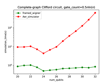
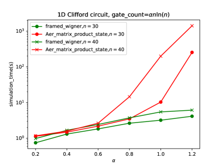
Figure 4: Comparison of simulation time for shallow Clifford circuits between framed Wigner function method and Qiskit Aer simulator. (a) Average time (over 10 random samples) of complete-graph Clifford circuit by framed Wigner function method and Aer_simulator. Here, the Aer_simulator seeks the most appropriate simulator backend among all the simulators the Aer_simulator package has. (b) Average time (over 10 random samples) of 1D Clifford circuit by framed Wigner function method and Aer_matrix_product_state simulator.

In this section, we show two graphs of the simulation speed of shallow non-adaptive Clifford circuits. See Fig. 4. We compare the simulation time between our simulator and the Qiskit Aer_simulator. For the Wigner function method, simulation time includes the frame changing and finding simulatable qubits (via greedy algorithm) as well as sampling and rotating the phase point. In both simulators, Wigner and Qiskit, we measure the marginal outcome only once. In Fig. 4 (a), we can see that our simulator executes the marginal sampling very fast while the time taken for the Aer_simulator increases exponentially by increasing the number of qubits. In Fig. 4 (b), we simulate 1D Clifford circuit with Aer_matrix_product_state (Aer_mps) simulator and compare the time with our method. The Aer_mps employs the tensor network method and is efficient for large but low-entangled circuits. We note that simulation time increases exponentially by increasing the scale factor of gate count, $\alpha$, hence by increasing the depth.

Up to 40 qubits, the number of simulatable qubits is not sufficiently large, so there exists a more trivial method, as we discussed after Theorem 2, and it manages a similar time scale. However, we can surely expect that this low time scaling of the Wigner function simulator lasts for larger $n$ (and larger simulatable qubits) with which such a trivial method does not work.

VII Section VI: More details on log-depth quantum circuits

VII.1 Circuit architecture

We first briefly explain the definitions of several Clifford circuit architectures [31]. One is the 1D architecture, where $n$ is even and the qubits are arranged on a ring and we put a random single qubit gate to each qubit and alternating layers of $n/2$ nearest-neighbor random Clifford gates. The other is the complete graph architecture, where we put a random single qubit gate to each qubit and randomly choose $i,j\in[n]$ and locate a 2-qubit random Clifford gate on $i,j$-th qubits, and repeat this procedure. Gate count is the total number of 2-qubit random Clifford gates. In both architectures, random choice is done uniformly and we locate each gate one by one until the gate count reaches the designated value. The depth of the circuit means the minimum value of the number of stages in which we can operate a set of 2-qubit gates at once. See Ref. [31] for a detailed definition. Furthermore, the authors in Ref. [31] showed that in both cases, there exists sufficient and necessary scaling of gate count $\mathcal{O}(n\log(n))$ such that outcome probability distribution of random circuit sampling (including random unitary gates) satisfies anti-concentration.

VII.2 On the simulatable qubits found from the Greedy algorithm for 1D circuits and time complexity

For a $\log$-depth 1D architecture, even if we do not use the framed Wigner formalism, we can always find a linear-scaled number of simulatable qubits. We briefly explain how to do it. Suppose we have a $d$-depth 1D circuit. Now, we pick $i\in[n]$ and choose one group of locations of qubits, $\left\{i-\lfloor\beta\log(n)\rfloor,i-(\lfloor\beta\log(n)\rfloor-1),\ldots,i,\ldots,i+(\lceil\beta\log(n)\rceil-1),i+\lceil\beta\log(n)\rceil\right\}$. Then if we only measure this subset of qubits, we can efficiently simulate it with rotating Pauli operators via Clifford operations [3] with at most $\mathcal{O}(n^{\beta+1}\log_{2}(n))$-time. Because one method is to exactly calculate the Born probability. To do so, we expand the target binary state by $2^{\beta\log_{2}(n)}=n^{\beta}$ number of coherent $Z$ operators and then obtain all traces between the input product state and Pauli operators, which is backward-evolved by Clifford circuit starting from those $Z$ operators. We note that each expectation is obtained in $\mathcal{O}(n\log_{2}(n)))$-time [3, 28]. Furthermore, if we choose another $i^{\prime}\in[n]$ such that $\left\{j-\lfloor\beta\log(n)\rfloor,j-(\lfloor\beta\log(n)\rfloor-1),\ldots,j,\ldots,j+(\lceil\beta\log(n)\rceil-1),j+\lceil\beta\log(n)\rceil\right\}$ is $2d$-far away from the previous group (see Fig. 5 for 3-depth case), then we can also efficiently simulate these measurements by same time complexity because gates involved in two simulations are totally separated. By repeating this logic, we can find $\frac{n}{2d+\beta\log_{2}(n)}$-number of simulatable groups. Hence, given $d=\alpha\log_{2}(n)$, the total number of simulatable qubits is $\frac{\beta n}{2\alpha+\beta}$, also total simulation time is $\mathcal{O}(n^{\beta+2})$.

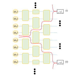
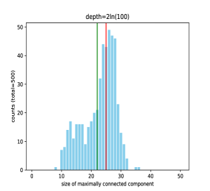
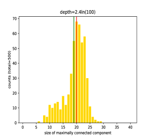
Figure 5: (a) Schematic illustration of a 3-depth 1D circuit. Measurement on (i)-th qubit does not influence the measurement outcome of (ii) (6-far away from (i)). If we only simulate these two measurements, we can separate this circuit into two portions sided by the red line. (b,c) The population of the size of maximally connected components for 500 numbers of 100-qubit 1D shallow Clifford samples. The green line represents the average size of maximally connected components, and the red line indicates the average value of total simulatable qubits of each sample. (b): Results of depth $=2\ln(100)$ 1D circuits (green line:22, red line:25). (c): Results of depth $=2.4\ln(100)$ 1D circuits (green line:19, red line:20).

This trivial method only finds distant groups in which measurements are stuck together. However, we can numerically check that in many cases, our methods find different types of measurements that are not far from each other. More precisely, given a non-adaptive Clifford circuit with the Clifford unitary $U$, let $A_{U}\equiv\left\{i_{1},i_{2},\ldots,i_{\left|A_{U}\right|}\right\}\subset[n]$ be set of locations of simulatable qubits. Now, let $Z_{i}$ be an n-qubit Paul operator which affects $Z$-operation to $i$-th qubit and identity to the other qubits. Now we calculate the set of Pauli operators $P_{A_{U}}\equiv\left\{U^{\dagger}Z_{i}U|i\in A_{U}\right\}$ which can be obtained efficiently [3]. Then we can define the 2-graph $G(A_{U},E_{A_{U}})$ where the set of vertex is $A_{U}$ and $E_{A_{U}}$ is set of edges which connects $i,j\in S$ if and only if two Pauli strings $U^{\dagger}Z_{i}U$ and $U^{\dagger}Z_{j}U$ have non-trivial (not identity, not need to be same) Pauli operation on the same qubit location. Now, we denote $\mathcal{C}(G(A_{U},E_{A_{U}}))\subset A_{U}$ as a set of connected components of $G$, i.e vertices consisting of connected subgraphs such that each subgraph is not connected with the others. Then we easily note that measurement on the set of qubits with location $C^{\prime}\in\mathcal{C}(G(A_{U},E_{A_{U}}))$ is independent of the measurement outcome of other locations in $\mathcal{C}(G(A_{U},E_{A_{U}}))$. Hence the time complexity of weak simulation can be bound by $\mathcal{O}\left(\exp\left({\max_{C\in\mathcal{C}(G(A_{U},E_{A_{U}}))}(\left|C\right|)}\right)\right)$, which can be achieved by the similar method with the first paragraph. Now we see Fig. 5 (b) and (c). We randomly sample 500 numbers of $100$-qubit 1D Clifford circuit $U$ with zero frame input and find $\max_{C\in\mathcal{C}(G(A_{U},E_{A_{U}}))}(\left|C\right|)$ efficiently via Python NetworkX packages, and we observed that most of the samples have many connected Pauli projectors $U^{\dagger}Z_{i}U\;(i\in A_{U})$ and hence such a trivial decomposition (in the first paragraph) is not applied to them.

Furthermore, from the result of Theorem 2, we note that total time to simulate $\log(n)$-depth 1D circuit is at most $\mathcal{O}(n\log(n))$ because we sample the phase point from the initial framed Wigner function in $\mathcal{O}(n)$-time and we take symplectic transform to it in $\mathcal{O}(n\log(n))$-time. Before that, we need to change the frame and solve the vertex cover problem (with approximative algorithms [27, 40]). However, we do not need to do those things over once. Furthermore, by Proposition. 1, frame changes in at most $\mathcal{O}(n(\log(n))^{4})+n^{2}\log(n))$-time, and the greedy algorithm can be done in $\mathcal{O}(n^{2}\log(n))$-time which is easily derived by Corollary 3 and locality of edges of resulting frame graph. Therefore, even the first trial has a shorter time given that $n^{\beta}\gg\log(n)$.

VII.3 Finite-sized scaling for log-depth completely connected circuits

Let us consider a random Clifford circuit and increase the number of qubits $n$ while fixing the scale factor ($\alpha$ in the main text) of the $\log$-depth. The average number of measurable qubits ($N_{sim}$) then increases by $n$. However, the increasing rates of $N_{sim}$ under $n$ might differ before and after passing the critical point, $\alpha_{c}$. In order to take this into account, we express $N_{sim}$ as a function of $\alpha$ and $n$,

$$N_{sim}(\alpha,n)-N_{sim}(\alpha_{c},n)=f((\alpha-\alpha_{c}),n),$$ (30)

for some function $f$ having different scaling at $\alpha<\alpha_{c}$ and $\alpha>\alpha_{c}$. We must note that $f(0,n)=0$ for all $n$.

Finite-sized scaling (FSS) gathers the data of $N_{sim}$ with various $\alpha$ and $n$ and infers the functions $f$ and $\alpha_{c}$. We take the ansatz $f((\alpha-\alpha_{c})n^{\frac{1}{\nu}})$ for some $\nu\in\mathbb{R}$ which is normally used in FSS literature [33]. Given many tuples of data $(\alpha,n,N_{sim}(\alpha,n))$, we fix $\nu$ and plot the graphs of $N_{sim}(\alpha,n)-N_{sim}(\alpha_{c},n)$ for each $n$ with $x$-axis as $(\alpha-\alpha_{c})n^{\frac{1}{\nu}}$. We repeat this procedure by changing the $\nu$ and $\alpha_{c}$ until all plots are on the same line and see the rate is drastically changed at zero point. See Fig. 3 (e) in the main text. After we find such $(\nu,\alpha_{c})$, we see that line from x-value $0$ to $-20$ is quasi-linear. It means that when $\alpha<\alpha_{c}$, the difference $\left|N_{sim}(\alpha,n)-N_{sim}(\alpha_{c},n)\right|$ increases quasi-linearly by increasing $n$. Whereas, the line from $x$-value $0$ to $20$ decreases very slowly. Hence for $\alpha>\alpha_{c}$ and increasing $n$, $\left|N_{sim}(\alpha,n)-N_{sim}(\alpha_{c},n)\right|$ increases with much smaller scale than the former one. Therefore, we can expect that there exists a transition of the scale of $N_{sim}$ around $\alpha=\alpha_{c}$.

References

Shor [1999]P. W. Shor, Polynomial-time algorithms
for prime factorization and discrete logarithms on a quantum computer, SIAM review 41, 303 (1999).
Nielsen and Chuang [2001]M. A. Nielsen and I. L. Chuang, Quantum computation and
quantum information, Phys. Today 54, 60 (2001).
Jozsa and Nest [2013]R. Jozsa and M. V. d. Nest, Classical simulation
complexity of extended clifford circuits, arXiv preprint arXiv:1305.6190 (2013).
Bravyi and Kitaev [2005]S. Bravyi and A. Kitaev, Universal quantum
computation with ideal clifford gates and noisy ancillas, Physical review A 71, 022316 (2005).
Mari and Eisert [2012]A. Mari and J. Eisert, Positive wigner functions render
classical simulation of quantum computation efficient, Physical review letters 109, 230503 (2012).
Veitch et al. [2012]V. Veitch, C. Ferrie,
D. Gross, and J. Emerson, Negative quasi-probability as a resource for quantum
computation, New Journal of Physics 14, 113011 (2012).
Veitch et al. [2013]V. Veitch, N. Wiebe,
C. Ferrie, and J. Emerson, Efficient simulation scheme for a class of quantum optics
experiments with non-negative wigner representation, New Journal of Physics 15, 013037 (2013).
Rahimi-Keshari et al. [2016]S. Rahimi-Keshari, T. C. Ralph, and C. M. Caves, Sufficient conditions for
efficient classical simulation of quantum optics, Physical review X 6, 021039 (2016).
Howard et al. [2014]M. Howard, J. Wallman,
V. Veitch, and J. Emerson, Contextuality supplies the ‘magic’for quantum
computation, Nature 510, 351 (2014).
Howard and Campbell [2017]M. Howard and E. Campbell, Application of a
resource theory for magic states to fault-tolerant quantum computing, Physical review letters 118, 090501 (2017).
Veitch et al. [2014]V. Veitch, S. H. Mousavian, D. Gottesman, and J. Emerson, The resource theory of
stabilizer quantum computation, New Journal of Physics 16, 013009 (2014).
Pashayan et al. [2015]H. Pashayan, J. J. Wallman, and S. D. Bartlett, Estimating outcome
probabilities of quantum circuits using quasiprobabilities, Physical review letters 115, 070501 (2015).
Koukoulekidis et al. [2022]N. Koukoulekidis, H. Kwon,
H. H. Jee, D. Jennings, and M. S. Kim, Faster Born probability estimation via gate merging and
frame optimisation, Quantum 6, 838 (2022).
Kocia and Love [2017]L. Kocia and P. Love, Discrete wigner formalism for qubits
and noncontextuality of clifford gates on qubit stabilizer states, Physical review A 96, 062134 (2017).
Raussendorf et al. [2017]R. Raussendorf, D. E. Browne, N. Delfosse,
C. Okay, and J. Bermejo-Vega, Contextuality and wigner-function negativity in
qubit quantum computation, Physical Review A 95, 052334 (2017).
Raussendorf et al. [2020]R. Raussendorf, J. Bermejo-Vega, E. Tyhurst, C. Okay, and M. Zurel, Phase-space-simulation method for quantum
computation with magic states on qubits, Physical Review A 101, 012350 (2020).
Zurel et al. [2020]M. Zurel, C. Okay, and R. Raussendorf, Hidden variable model for universal
quantum computation with magic states on qubits, Physical review letters 125, 260404 (2020).
Zurel et al. [2023]M. Zurel, C. Okay, and R. Raussendorf, Simulating quantum computation with magic
states: how many ”bits” for ”it”? (2023), arXiv:2305.17287 [quant-ph] .
Bouland et al. [2017]A. Bouland, J. F. Fitzsimons, and D. E. Koh, Complexity classification of
conjugated clifford circuits, arXiv preprint arXiv:1709.01805 (2017).
Bu and Koh [2019]K. Bu and D. E. Koh, Efficient classical simulation of
clifford circuits with nonstabilizer input states, Phys. Rev. Lett. 123, 170502 (2019).
Dalzell et al. [2022]A. M. Dalzell, N. Hunter-Jones, and F. G. S. L. Brandão, Random
quantum circuits anticoncentrate in log depth, PRX Quantum 3, 010333 (2022).
Napp et al. [2022]J. C. Napp, R. L. La Placa,
A. M. Dalzell, F. G. S. L. Brandão, and A. W. Harrow, Efficient classical simulation of random shallow
2d quantum circuits, Physical review X 12, 021021 (2022).
Skinner et al. [2019]B. Skinner, J. Ruhman, and A. Nahum, Measurement-induced phase transitions in the
dynamics of entanglement, Physical review X 9, 031009 (2019).
Pashayan et al. [2020]H. Pashayan, S. D. Bartlett, and D. Gross, From estimation of quantum
probabilities to simulation of quantum circuits, Quantum 4, 223 (2020).
Bouland et al. [2019]A. Bouland, B. Fefferman,
C. Nirkhe, and U. Vazirani, On the complexity and verification of quantum random
circuit sampling, Nature Physics 15, 159 (2019).
Jiang et al. [2022]J. Jiang, X. Sun, S.-H. Teng, B. Wu, K. Wu, and J. Zhang, Optimal
space-depth trade-off of cnot circuits in quantum logic synthesis (2022), arXiv:1907.05087
[quant-ph] .
Bravyi et al. [2019]S. Bravyi, D. Browne,
P. Calpin, E. Campbell, D. Gosset, and M. Howard, Simulation of quantum circuits by low-rank stabilizer
decompositions, Quantum 3, 181 (2019).
Bremner et al. [2016]M. J. Bremner, A. Montanaro, and D. J. Shepherd, Average-case complexity versus
approximate simulation of commuting quantum computations, Physical review letters 117, 080501 (2016).