Quantum local-equilibrium state with fixed multiplicity constraint and Bose-Einstein momentum correlations

Abstract

The one- and two-boson momentum spectra are derived in the quantum local-equilibrium canonical ensemble of noninteracting bosons with a fixed particle number constraint. We define the canonical ensemble as a subensemble of events associated with the grand-canonical ensemble. Applying simple hydro-inspired parametrization with parameter values that correspond roughly to the values at the system’s breakup in $p+p$ collisions at the LHC energies, we compare our findings with the treatment which is based on the grand-canonical ensembles where mean particle numbers coincide with fixed particle numbers in the canonical ensembles. We observe a significantly greater sensitivity of the two-particle momentum correlation functions to fixed multiplicity constraint compared to one-particle momentum spectra. The results of our analysis may be useful for interpretation of multiplicity-dependent measurements of $p+p$ collision events.

I Introduction

Inasmuch as mean particle multiplicities in relativistic heavy ion collisions are large, the whole set of collision events at a fixed energy of nuclear collisions is typically divided into subsets with fixed charged-particle multiplicities. Corresponding multiplicity classes are associated with collision centralities and, thereby, with the initial system’s geometry which is primarily characterized by the overall shape of the interaction region. This makes it possible to study the multiplicity dependence of various observables measured at the same energy of collisions. In particular, the fixed particle multiplicity technique has been utilized for analysis of the Bose-Einstein momentum correlations of identical particles. These correlations are typically represented in terms of the interferometry radii. They are the result of the Gaussian fit of the correlation function defined as a ratio of the two-particle spectra to the product of the single-particle ones. These radii reflect the space-time structure and dynamical evolution of the systems created in nuclear collisions (for review of the correlation femtoscopy method see e.g. Ref. Sin-1 ). One notable feature of these measurements is that the effective system’s volume, when extracted from the Gaussian interferometry radii, appears to scale nearly linearly with charged particle multiplicity (see e.g. Ref. (Alice )). This observation is in agreement with the hydrodynamical picture of nuclear collisions.

Recently, because of the start of LHC experiments, the fixed particle multiplicity technique has been utilized for analysis of the Bose-Einstein momentum correlations of identical particles in proton-proton collisions at a fixed energy of collisions. It was observed, in particular, that measured in these collisions interferometry correlation radius parameters do not increase with multiplicity at high charged-particle multiplicities Atlas ; CMS . While an explanation of this effect is still absent, it is suggestive to assume that the saturation effect in the multiplicity dependence of the interferometry correlation radius parameters takes place once the maximal overlap of colliding nucleons is achieved in most central collisions. Indeed, the color glass condensate effective theory predicts that once maximal overlap is achieved higher multiplicities can only be reached by certain color charge fluctuations, which do not increase the initial size of the system Lerran . Then, one can speculate that an individual system created in a high-multiplicity $p+p$ collision can be regarded as an element of a quantum-statistical ensemble of systems with various numbers of particles produced under the same initial-state geometry.

In a quantum-statistical framework, observables are the expectation values of the corresponding quantum operators with respect to a suitable statistical operator. For example, successful applicability of almost perfect relativistic hydrodynamics for the description of a particle production in relativistic heavy ion collisions (for a recent review see, e.g., Ref. Schen ) indicates that actual state of a system created in collisions with the same centrality can be approximated by a local-equilibrium statistical operator $\rho^{\text{leq}}$, $\rm{Tr}[\rho^{\text{leq}}]=1$, which is obtained by maximizing the von Neumann entropy, $S=-{\rm Tr}[\rho\ln{\rho}]$, with constrained mean values of energy-momentum and conserved charge densities on a given three-dimensional hypersurface (see, e.g., Ref. Zubarev ). It is noteworthy that high-multiplicity proton-proton collisions exhibit collective behavior similar to that observed in relativistic nuclear collisions. It indicates that a hydrodynamic description of matter formed in these collisions might also be possible Schen . Application of fixed high-multiplicity constraint to $p+p$ collision events means then selecting some subensemble of events with the same initial-state geometry to which the considered system belongs. To assign a quantum statistical state to a subensemble of events with fixed multiplicity, one can utilize the projection operator ${\cal P}_{N}$, which automatically invokes such a constraint. The aim of this work (see also Ref. Akkelin-2 ) is to clarify how imposed particle number constraint affects the one-particle spectra and two-boson momentum correlations in a quantum-field local-equilibrium state. It is worth noting that for fairly high particle numbers a canonical ground-state Bose-Einstein condensation can occur. Such a condensation could, in principle, lead to noticeable effects in particle momentum spectra and correlations at fixed multiplicities. This issue is, however, beyond the scope of this paper.

II Local-equilibrium statistical operator

As a starting point, we consider the quasiequilibrium state (see, e.g., Ref. Zubarev ) of a real relativistic scalar field. This state is represented by the statistical operator $\rho^{\text{q}}(\sigma)$ as (we use the convention $g^{\mu\nu}=\mbox{diag}(+1,-1,-1,-1)$)

$$\rho^{\text{q}}(\sigma)=\frac{1}{Z^{\text{q}}(\sigma)}\hat{\rho}^{\text{q}}(\sigma),$$ (1)

$$\hat{\rho}^{\text{q}}(\sigma)=\exp\left(-\int_{\sigma}d\sigma n_{\mu}(x)\beta_{\nu}(x)T^{\mu\nu}(x)\right),$$ (2)

where $\sigma$ is a three-dimensional spacelike hypersurface with a timelike normal vector $n_{\mu}(x)$; $\beta_{\nu}(x)=\beta(x)u_{\nu}(x)$, $u_{\mu}(x)u^{\mu}(x)=1$ are the corresponding Lagrange multipliers ($\beta=1/T$ is the inverse temperature, and $u_{\mu}$ is the $4$-velocity) on the hypersurface $\sigma$, adjusted such as to satisfy the actual mean values of energy and momentum density at this hypersurface; $Z^{\text{q}}(\sigma)$ is the normalization factor making $\rm{Tr}[\rho^{\text{q}}(\sigma)]=1$; and $T^{\mu\nu}(x)$ is a scalar-field energy-momentum tensor. For simplicity, we disregard field self-interactions and consider a noninteracting scalar quantum field model. Then, the $T^{\mu\nu}(x)$ reads

$$T^{\mu\nu}(x)=\partial^{\mu}\phi\partial^{\nu}\phi-g^{\mu\nu}L,$$ (3)

where the Lagrangian density is

$$L=\frac{1}{2}\left(\frac{\partial\phi}{\partial t}\right)^{2}-\frac{1}{2}\left(\frac{\partial\phi}{\partial\textbf{r}}\right)^{2}-\frac{m^{2}}{2}\phi^{2}.$$ (4)

Here

$$\phi(x)=\int\frac{d^{3}p}{\sqrt{2\omega_{p}}}\frac{1}{(2\pi)^{3/2}}\left(e^{-i\omega_{p}t+i\textbf{p}\textbf{r}}a(\textbf{p})+e^{i\omega_{p}t-i\textbf{p}\textbf{r}}a^{{\dagger}}(\textbf{p})\right),$$ (5)

and

$$\omega_{p}=\sqrt{\textbf{p}^{2}+m^{2}}.$$ (6)

The quantization prescription means that $a^{{\dagger}}(\textbf{p})$ and $a(\textbf{p})$ are creation and annihilation operators, respectively, which satisfy the following canonical commutation relations:

$$[a(\textbf{p}),a^{{\dagger}}(\textbf{p}^{\prime})]=\delta^{(3)}(\textbf{p}-\textbf{p}^{\prime})$$ (7)

and $[a(\textbf{p}),a(\textbf{p}^{\prime})]=[a^{{\dagger}}(\textbf{p}),a^{{\dagger}}(\textbf{p}^{\prime})]=0$.

Before proceeding further, let us digress for a moment and consider the simple case of the covariant global-equilibrium state, where the $\beta_{\mu}$ does not depend on spacetime coordinates across the infinite three-dimensional hypersurface. Then the statistical operator reads

$$\rho^{\text{eq}}=\frac{1}{Z^{\text{eq}}}\exp\left(-\beta_{\mu}P^{\mu}\right),$$ (8)

where $P^{\mu}=\int_{t}d^{3}rT^{\mu 0}(x)$ is $4$-momentum of the field defined at $t=\text{const}$ hypersurface. Then, using Eqs. (3), (4), and (5), we obtain

$$P^{\mu}=\frac{1}{2}\int d^{3}kk^{\mu}(a^{{\dagger}}(\textbf{k})a(\textbf{k})+a(\textbf{k})a^{{\dagger}}(\textbf{k})).$$ (9)

It is convenient to introduce

$$P^{\mu}_{\text{reg}}=P^{\mu}-\langle 0|P^{\mu}|0\rangle=\int d^{3}kk^{\mu}a^{{\dagger}}(\textbf{k})a(\textbf{k}),$$ (10)

where $|0\rangle$ is the quantum field vacuum state, $a(\textbf{p})|0\rangle=0$. Then, Eq. (8) can be rewritten as

$$\rho^{\text{eq}}=\frac{1}{Z^{\text{eq}}_{\text{reg}}}\exp\left(-\beta_{\mu}P^{\mu}_{\text{reg}}\right).$$ (11)

It can be shown, e.g., by Gaudin’s method Gaudin , that the statistical operator (11) is associated with the homogeneous ideal gas Bose distribution,

$$f_{\text{eq}}(p)=\frac{1}{(2\pi)^{3}}\frac{1}{e^{\beta_{\nu}p^{\nu}}-1}.$$ (12)

Below, for the reader’s convenience, we present an elementary derivation of it (see also Ref. Groot ). Let us start by defining $a(\textbf{p},\alpha)$,

$$a(\textbf{p},\alpha)=\exp\left(\alpha\beta_{\mu}P^{\mu}_{\text{reg}}\right)a(\textbf{p})\exp\left(-\alpha\beta_{\mu}P^{\mu}_{\text{reg}}\right).$$ (13)

Note that $a(\textbf{p},0)=a(\textbf{p})$. Expression (13) implies that $a(\textbf{p},\alpha)$ satisfies equation

$$\frac{\partial a(\textbf{p},\alpha)}{\partial\alpha}=\left[\beta_{\mu}P^{\mu}_{\text{reg}},a(\textbf{p},\alpha)\right].$$ (14)

Taking into account that

$$\left[\beta_{\mu}P^{\mu}_{\text{reg}},a(\textbf{p},\alpha)\right]=\exp\left(\alpha\beta_{\mu}P^{\mu}_{\text{reg}}\right)\left[\beta_{\mu}P^{\mu}_{\text{reg}},a(\textbf{p})\right]\exp\left(-\alpha\beta_{\mu}P^{\mu}_{\text{reg}}\right),$$ (15)

this yields then

$$\frac{\partial a(\textbf{p},\alpha)}{\partial\alpha}=-\beta_{\mu}p^{\mu}a(\textbf{p},\alpha).$$ (16)

The solution of this equation is

$$a(\textbf{p},\alpha)=a(\textbf{p})\exp{(-\alpha\beta_{\mu}p^{\mu})}.$$ (17)

Our next step is to combine the cyclic invariance of the trace, $\rm{Tr}[\rho^{\text{eq}}(\sigma)a^{{\dagger}}(\textbf{p}_{1})a(\textbf{p}_{2})]$, and Eqs. (13) and (17). Using the cyclic invariance of the trace and Eq. (13), we obtain

$$\rm{Tr}[\rho^{\text{eq}}(\sigma)a^{{\dagger}}(\textbf{p}_{1})a(\textbf{p}_{2})]=\rm{Tr}[a(\textbf{p}_{2})\rho^{\text{eq}}(\sigma)a^{{\dagger}}(\textbf{p}_{1})]=$$

$$\rm{Tr}[\rho^{\text{eq}}(\sigma)a(\textbf{p}_{2},1)a^{{\dagger}}(\textbf{p}_{1})].$$ (18)

Taking into account Eqs. (7) and (17), the r.h.s. of the above equation can be rewritten as

$$\rm{Tr}[\rho^{\text{eq}}(\sigma)a(\textbf{p}_{2},1)a^{{\dagger}}(\textbf{p}_{1})]=\rm{Tr}[\rho^{\text{eq}}(\sigma)a^{{\dagger}}(\textbf{p}_{1})a(\textbf{p}_{2},1)]+[a(\textbf{p}_{2},1),a^{{\dagger}}(\textbf{p}_{1})]=$$

$$e^{-\beta_{\mu}p^{\mu}_{2}}\left(\rm{Tr}[\rho^{\text{eq}}(\sigma)a^{{\dagger}}(\textbf{p}_{1})a(\textbf{p}_{2})]+\delta^{(3)}(\textbf{p}_{2}-\textbf{p}_{1})\right).$$ (19)

Substituting this into Eq. (18) we finally have

$$\rm{Tr}[\rho^{\text{eq}}(\sigma)a^{{\dagger}}(\textbf{p}_{1})a(\textbf{p}_{2})]=\delta^{(3)}(\textbf{p}_{1}-\textbf{p}_{2})\frac{1}{e^{\beta_{\nu}(p_{1}^{\nu}+p_{2}^{\nu})/2}-1}.$$ (20)

Utilization of the Fourier transformation of Eq. (20) with respect to $\Delta\textbf{p}=\textbf{p}_{2}-\textbf{p}_{1}$ immediately results in the ideal gas Bose distribution function (12).

Now, going back to the quasiequilibrium statistical operator (1), (2), we suppose that $\beta(x)$ and $u_{\mu}(x)$ are slowly varying functions across the three-dimensional hypersurface $\sigma$. This makes it possible to apply a local thermal equilibrium approximation (see, e.g., Refs. Zubarev ; Fl ) of the statistical operator (1), (2). The local thermal equilibrium is an approximate concept which is usually associated with the possibility of defining a fluid cell, i.e., with the existence of a scale at which the system appears to be at homogeneous equilibrium. Therefore, this scale should be much smaller than the distance over which the $\beta_{\mu}(x)=\beta(x)u_{\mu}(x)$ varies essentially. On the other hand, this scale has to be assumed large enough from a microscopic point of view, meaning that the typical microscopic correlation lengths are much smaller than the size of a cell.

To avoid additional complications and formulate the idea more concretely, we restrict ourselves to the case when the timelike normal vector $n_{\mu}(x)$ of the hypersurface $\sigma$ coincides with the $4$-velocity field $u_{\mu}(x)$,

$$n_{\mu}(x)=u_{\mu}(x).$$ (21)

Then, we replace the integral in Eq. (2) by the sum as

$$\int_{\sigma}d\sigma n_{\mu}(x)\beta_{\nu}(x)T^{\mu\nu}(x))\approx\sum_{s}\beta_{\nu}(x_{s})P^{\nu}(\sigma_{s}),$$ (22)

where

$$P^{\nu}(\sigma_{s})=\int_{\sigma_{s}}d\sigma_{\mu}T^{\mu\nu}(x)\approx u_{\mu}(x_{s})\int_{\sigma_{s}}d\sigma T^{\mu\nu}(x),$$ (23)

and the integral in the above equation is taken over the homogeneity region of the $\beta_{\nu}(x)$ around some point $x_{s}^{\mu}$. The homogeneity region is defined as a region of the three-dimensional hypersurface $\sigma$ where $\beta_{\nu}(x)$ does not vary in a noticeable way. It is instructive to rewrite $\beta_{\nu}(x_{s})P^{\nu}(\sigma_{s})$ in the comoving coordinate system where $\tilde{u}_{\mu}(\tilde{x}_{s})=(1,\textbf{0})$. Then,

$$\beta_{\nu}(x_{s})P^{\nu}(\sigma_{s})=\tilde{\beta}_{0}(\tilde{x}_{s})\tilde{P}^{0}(\tilde{\sigma}_{s}),$$ (24)

$$\tilde{P}^{0}(\tilde{\sigma}_{s})=\int_{\tilde{t}_{s}}d^{3}\tilde{r}T^{00}(\tilde{x}),$$ (25)

$$\tilde{\beta}_{0}(\tilde{x}_{s})=\beta(x_{s}),$$ (26)

and $\tilde{t}_{s}=\text{const}$. The key assumption underlying the local-equilibrium approximation is that characteristic size, $\tilde{L}$, of the corresponding volume element is large enough, i.e., $\tilde{L}\gg 1/m$. This assumption has important consequences. In particular, by using Eqs. (3), (4), and (5), one can show that contributions of $aa$ and $a^{{\dagger}}a^{{\dagger}}$ terms to the $\tilde{P}^{0}(\tilde{\sigma}_{s})$ can be neglected. In a sense, this provides the local thermal equilibrium in the region $s$ around $x_{s}^{\mu}$. The corresponding local-equilibrium statistical operator is

$$\rho^{\text{leq}}(\sigma)=\frac{1}{Z^{\text{leq}}_{\text{reg}}(\sigma)}\hat{\rho}^{\text{leq}}(\sigma),$$ (27)

$$\hat{\rho}^{\text{leq}}(\sigma)=\exp\left(-\sum_{s}\beta_{\nu}(\sigma_{s})P^{\nu}_{\text{reg}}(\sigma_{s})\right),$$ (28)

where $P^{\mu}_{\text{reg}}(\sigma_{s})=P^{\mu}(\sigma_{s})-\langle 0|P^{\mu}(\sigma_{s})|0\rangle$. By using Eqs. (3), (4), and (5), we get

$$\beta_{\nu}(\sigma_{s})P^{\nu}_{\text{reg}}(\sigma_{s})\approx$$

$$\beta(\sigma_{s})\int\frac{d^{3}k}{k_{0}}\frac{d^{3}k^{\prime}}{k^{\prime}_{0}}\frac{u_{\mu}(x_{s})k^{\mu}u_{\nu}(x_{s})k^{\prime\nu}}{(2\pi)^{3}}\int_{\sigma_{s}}d\sigma e^{i(k-k^{\prime})x}\sqrt{k_{0}k^{\prime}_{0}}a^{{\dagger}}(\textbf{k})a(\textbf{k}^{\prime}).$$ (29)

Going to the local rest frame for a cell, we can write Eq. (29) in the following form:

$$\beta(x_{s})\tilde{P}^{0}_{\text{reg}}(\tilde{\sigma}_{s})\approx\beta(\sigma_{s})\int d^{3}\tilde{k}d^{3}\tilde{k}^{\prime}\frac{1}{(2\pi)^{3}}\int_{\tilde{t}_{s}}d^{3}\tilde{r}e^{i(\tilde{k}-\tilde{k}^{\prime})\tilde{x}}\sqrt{\tilde{k}_{0}\tilde{k}^{\prime}_{0}}a^{{\dagger}}(\tilde{\textbf{k}})a(\tilde{\textbf{k}}^{\prime}).$$ (30)

Equation (29) makes possible to rewrite the operator $\sum_{s}\beta_{\nu}(\sigma_{s})P^{\nu}_{\text{reg}}(\sigma_{s})$ as

$$\sum_{s}\beta_{\nu}(\sigma_{s})P^{\nu}_{\text{reg}}(\sigma_{s})\approx\int d^{3}kd^{3}k^{\prime}A(\textbf{k},\textbf{k}^{\prime},\sigma)a^{{\dagger}}(\textbf{k})a(\textbf{k}^{\prime}),$$ (31)

where

$$A(\textbf{k},\textbf{k}^{\prime},\sigma)=\sum_{s}A_{s}(\textbf{k},\textbf{k}^{\prime},\sigma),$$ (32)

$$A_{s}(\textbf{k},\textbf{k}^{\prime},\sigma)=\beta(\sigma_{s})\frac{1}{\sqrt{k_{0}k^{\prime}_{0}}}\frac{u_{\mu}(x_{s})k^{\mu}u_{\nu}(x_{s})k^{\prime\nu}}{(2\pi)^{3}}\int_{\sigma_{s}}d\sigma e^{i(k-k^{\prime})x}.$$ (33)

III Quantum local-equilibrium grand-canonical ensemble

In this section, we calculate one-particle and two-particle momentum spectra in the grand-canonical ensemble, which is described by the local-equilibrium statistical operator. For this aim, it is convenient to compute fist $\langle a^{{\dagger}}(\textbf{p}_{1})a(\textbf{p}_{2})\rangle$, where $\langle...\rangle=\rm{Tr}[...\rho^{\text{leq}}(\sigma)]$. It can be done by adapting the Gaudin’s method to our problem. We start by defining $a(\textbf{p},\alpha)$, $a(\textbf{p},0)=a(\textbf{p})$, $\rm{Im}(\alpha)=0$, as

$$a(\textbf{p},\alpha)=\exp\left(\alpha\sum_{s}\beta_{\nu}(\sigma_{s})P^{\nu}_{\text{reg}}(\sigma_{s})\right)a(\textbf{p})\exp\left(-\alpha\sum_{s}\beta_{\nu}(\sigma_{s})P^{\nu}_{\text{reg}}(\sigma_{s})\right),$$ (34)

where $\sum_{s}\beta_{\nu}(\sigma_{s})P^{\nu}_{\text{reg}}(\sigma_{s})$ is defined by Eqs. (31), (32), and (33). Applying the operator identity

$$e^{X}Ye^{-X}=Y+\left[X,Y\right]+\frac{1}{2!}\left[X,\left[X,Y\right]\right]+\frac{1}{3!}\left[X,\left[X,\left[X,Y\right]\right]\right]+...,$$ (35)

we can write the result as

$$a(\textbf{p},\alpha)=a(\textbf{p})+(-\alpha)\int d^{3}kA(\textbf{p},\textbf{k},\sigma)a(\textbf{k})+$$

$$\frac{(-\alpha)^{2}}{2!}\int d^{3}k_{1}d^{3}kA(\textbf{p},\textbf{k}_{1},\sigma)A(\textbf{k}_{1},\textbf{k},\sigma)a(\textbf{k})+$$

$$\frac{(-\alpha)^{3}}{3!}\int d^{3}k_{1}d^{3}k_{2}d^{3}kA(\textbf{p},\textbf{k}_{1},\sigma)A(\textbf{k}_{1},\textbf{k}_{2},\sigma)A(\textbf{k}_{2},\textbf{k},\sigma)a(\textbf{k})+....$$ (36)

Taking into account the nonoverlapping of different cells and neglecting the surface effect on the boundaries of neighboring cells, we get

$$a(\textbf{p},\alpha)\approx a(\textbf{p})+(-\alpha)\sum_{s}\int d^{3}kA_{s}(\textbf{p},\textbf{k},\sigma)a(\textbf{k})+$$

$$\frac{(-\alpha)^{2}}{2!}\sum_{s}\int d^{3}k_{1}d^{3}kA_{s}(\textbf{p},\textbf{k}_{1},\sigma)A_{s}(\textbf{k}_{1},\textbf{k},\sigma)a(\textbf{k})+$$

$$\frac{(-\alpha)^{3}}{3!}\sum_{s}\int d^{3}k_{1}d^{3}k_{2}d^{3}kA_{s}(\textbf{p},\textbf{k}_{1},\sigma)A_{s}(\textbf{k}_{1},\textbf{k}_{2},\sigma)A_{s}(\textbf{k}_{2},\textbf{k},\sigma)a(\textbf{k})+....$$ (37)

Substituting Eq. (33) into Eq. (37) and going to the local rest frame for each cell, we can perform an approximate integration over the momenta assuming that $\tilde{L}\gg 1/m$, where $\tilde{L}$ is the characteristic length scale of a cell. The result written in the laboratory coordinate system is

$$a(\textbf{p},\alpha)\approx a(\textbf{p})+(-\alpha)\sum_{s}\int d^{3}kA_{s}(\textbf{p},\textbf{k},\sigma)a(\textbf{k})+$$

$$\frac{(-\alpha)^{2}}{2!}\sum_{s}\int d^{3}k\left(\frac{(p^{\nu}+k^{\nu})}{2}\beta_{\nu}(\sigma_{s})\right)A_{s}(\textbf{p},\textbf{k},\sigma)a(\textbf{k})+$$

$$\frac{(-\alpha)^{3}}{3!}\sum_{s}\int d^{3}k\left(\frac{(p^{\nu}+k^{\nu})}{2}\beta_{\nu}(\sigma_{s})\right)^{2}A_{s}(\textbf{p},\textbf{k},\sigma)a(\textbf{k})+....$$ (38)

Taking into account that main contribution in the integral over k is given by $\textbf{k}\approx\textbf{p}$, it is convenient to substitute $u_{\mu}(x_{s})p^{\mu}u_{\nu}(x_{s})k^{\nu}$ in the $A_{s}(\textbf{p},\textbf{k},\sigma)$ by $((p^{\nu}+k^{\nu})u_{\nu}(x_{s})/2)^{2}$. The result is

$$a(\textbf{p},\alpha)\approx a(\textbf{p})+(-\alpha)\sum_{s}\int d^{3}k\left(\frac{(p^{\nu}+k^{\nu})}{2}\beta_{\nu}(\sigma_{s})\right)\delta^{(3)}_{s}(\textbf{p}-\textbf{k})a(\textbf{k})+$$

$$\frac{(-\alpha)^{2}}{2!}\sum_{s}\int d^{3}k\left(\frac{(p^{\nu}+k^{\nu})}{2}\beta_{\nu}(\sigma_{s})\right)^{2}\delta^{(3)}_{s}(\textbf{p}-\textbf{k})a(\textbf{k})+$$

$$\frac{(-\alpha)^{3}}{3!}\sum_{s}\int d^{3}k\left(\frac{(p^{\nu}+k^{\nu})}{2}\beta_{\nu}(\sigma_{s})\right)^{3}\delta^{(3)}_{s}(\textbf{p}-\textbf{k})a(\textbf{k})+...,$$ (39)

where we introduced notation

$$\delta^{(3)}_{s}(\textbf{p}-\textbf{k})=\frac{u_{\mu}(x_{s})}{(2\pi)^{3}}\int_{\sigma_{s}}d\sigma\frac{(p^{\mu}+k^{\mu})}{2\sqrt{\omega_{p}\omega_{k}}}e^{i(p-k)x}.$$ (40)

Note that the first term in Eq. (39) may be written as

$$a(\textbf{p})=\int d^{3}k\delta^{(3)}(\textbf{p}-\textbf{k})a(\textbf{k})\approx\int d^{3}k\sum_{s}\delta^{(3)}_{s}(\textbf{p}-\textbf{k})a(\textbf{k}).$$ (41)

Substituting (41) into (39), we obtain

$$a(\textbf{p},\alpha)\approx\sum_{n=0}^{\infty}\frac{(-\alpha)^{n}}{n!}\sum_{s}\int d^{3}k\left(\frac{k^{\nu}+p^{\nu}}{2}\beta_{\nu}(\sigma_{s})\right)^{n}\delta^{(3)}_{s}(\textbf{p}-\textbf{k})a(\textbf{k}).$$ (42)

It is convenient to introduce notation

$$G_{\alpha}^{*}(\textbf{p},\textbf{k},\sigma)=\sum_{s}\exp\left(-\alpha\beta_{\mu}(\sigma_{s})\frac{k^{\mu}+p^{\mu}}{2}\right)\delta^{(3)}_{s}(\textbf{p}-\textbf{k}),$$ (43)

and rewrite Eq. (42) in the form

$$a(\textbf{p},\alpha)\approx\int d^{3}kG_{\alpha}^{*}(\textbf{p},\textbf{k},\sigma)a(\textbf{k}).$$ (44)

From Eq. (43), we have that

$$G_{\alpha}^{*}(\textbf{p},\textbf{k},\sigma)=G_{\alpha}(\textbf{k},\textbf{p},\sigma)$$ (45)

and that

$$\int d^{3}kG_{\alpha_{1}}^{*}(\textbf{p}_{2},\textbf{k},\sigma)G_{\alpha_{2}}^{*}(\textbf{k},\textbf{p}_{1},\sigma)\approx G_{\alpha_{1}+\alpha_{2}}^{*}(\textbf{p}_{2},\textbf{p}_{1},\sigma).$$ (46)

We can now employ the cyclic invariance of the trace to get expression for $\langle a^{{\dagger}}(\textbf{p}_{1})a(\textbf{p}_{2})\rangle$. By using Eq. (34) and the cyclic invariance of the trace, one can write

$$Tr[\rho^{\text{leq}}(\sigma)a^{{\dagger}}(\textbf{p}_{1})a(\textbf{p}_{2})]=Tr[\rho^{\text{leq}}(\sigma)a(\textbf{p}_{2},1)a^{{\dagger}}(\textbf{p}_{1})]=$$

$$Tr[\rho^{\text{leq}}(\sigma)a^{{\dagger}}(\textbf{p}_{1})a(\textbf{p}_{2},1)]+[a(\textbf{p}_{2},1),a^{{\dagger}}(\textbf{p}_{1})].$$ (47)

Here, $a(\textbf{p}_{2},1)$ is given by Eq. (44). By using Eq. (44), we can write

$$[a(\textbf{p}_{2},1),a^{{\dagger}}(\textbf{p}_{1})]=G_{1}^{*}(\textbf{p}_{2},\textbf{p}_{1},\sigma).$$ (48)

Then, Eq. (47) becomes

$$\langle a^{{\dagger}}(\textbf{p}_{1})a(\textbf{p}_{2})\rangle=Tr[\rho^{\text{leq}}(\sigma)a^{{\dagger}}(\textbf{p}_{1})a(\textbf{p}_{2})]=$$

$$\int d^{3}kG_{1}^{*}(\textbf{p}_{2},\textbf{k},\sigma)\langle a^{{\dagger}}(\textbf{p}_{1})a(\textbf{k})\rangle+G_{1}^{*}(\textbf{p}_{2},\textbf{p}_{1},\sigma).$$ (49)

This equation can be solved by iteration. The result is

$$\langle a^{{\dagger}}(\textbf{p}_{1})a(\textbf{p}_{2})\rangle=G_{1}^{*}(\textbf{p}_{2},\textbf{p}_{1},\sigma)+\int d^{3}kG_{1}^{*}(\textbf{p}_{2},\textbf{k},\sigma)G_{1}^{*}(\textbf{k},\textbf{p}_{1},\sigma)+....$$ (50)

Taking into account (46) we get

$$\langle a^{{\dagger}}(\textbf{p}_{1})a(\textbf{p}_{2})\rangle=\sum_{n=1}^{\infty}G_{n}^{*}(\textbf{p}_{2},\textbf{p}_{1},\sigma),$$ (51)

where $G_{n}^{*}$ is given by Eq. (43). Substituting $G_{n}^{*}$ into Eq. (51), we have

$$\langle a^{{\dagger}}(\textbf{p}_{1})a(\textbf{p}_{2})\rangle\approx\sum_{s}\frac{1}{\exp\left(\frac{(p^{\nu}_{1}+p^{\nu}_{2})}{2}\beta_{\nu}(\sigma_{s})\right)-1}\delta^{(3)}_{s}(\textbf{p}_{1}-\textbf{p}_{2}).$$ (52)

Our next step is to replace sums over cells with integral over the hypersurface $\sigma$. This leads to

$$G_{n}(\textbf{p}_{1},\textbf{p}_{2},\sigma)\approx\frac{1}{(2\pi)^{3}\sqrt{p^{0}_{1}p^{0}_{2}}}\int_{\sigma}d\sigma_{\mu}p^{\mu}e^{-i(p_{1}-p_{2})x}e^{-n\beta_{\nu}(x)p^{\nu}},$$ (53)

$$\langle a^{{\dagger}}(\textbf{p}_{1})a(\textbf{p}_{2})\rangle\approx\frac{1}{(2\pi)^{3}\sqrt{p^{0}_{1}p^{0}_{2}}}\int_{\sigma}d\sigma_{\mu}p^{\mu}e^{-i(p_{1}-p_{2})x}\frac{1}{e^{\beta_{\nu}(x)p^{\nu}}-1},$$ (54)

where $p^{\mu}=(p^{\mu}_{1}+p^{\mu}_{2})/2$. One-particle momentum spectra then read

$$p_{0}\frac{d^{3}\langle N\rangle}{d^{3}p}=p_{0}\langle a^{{\dagger}}(\textbf{p})a(\textbf{p})\rangle\approx\int_{\sigma}d\sigma_{\mu}p^{\mu}f^{\text{leq}}(x,p),$$ (55)

where $f^{\text{leq}}(x,p)$ is the grand-canonical distribution function, which has the familiar form of the local-equilibrium distribution function of the relativistic ideal gas of bosons,

$$f^{\text{leq}}(x,p)=\frac{1}{(2\pi)^{3}}\frac{1}{e^{\beta_{\nu}(x)p^{\nu}}-1}.$$ (56)

It is worth noting that our derivation can be readily extended to the local-equilibrium grand-canonical ensemble with nonzero constant chemical potential, $\mu$, associated with mean number of particles. Then, $u_{\nu}(x)p^{\nu}\rightarrow u_{\nu}(x)p^{\nu}-\mu$.

Evidently, our derivation is rather heuristic and nonrigorous. But, in our opinion, it is instructive and adds some insights into the consistency of the approximations needed to associate quasiequilibrium statistical operator $\rho^{\text{q}}$ with the local-equilibrium ideal Bose gas distribution $f_{\text{leq}}(x,p)$.

Proceeding in the same way as above, one can readily derive an expression for the two-particle momentum spectra,

$$p^{0}_{1}p^{0}_{2}\frac{d^{6}\langle N(N-1)\rangle}{d^{3}p_{1}d^{3}p_{2}}=p^{0}_{1}p^{0}_{2}\langle a^{{\dagger}}(\textbf{p}_{1})a^{{\dagger}}(\textbf{p}_{2})a(\textbf{p}_{1})a(\textbf{p}_{2})\rangle.$$ (57)

We start by using the cyclic invariance of the trace. This leads to

$$\langle a^{{\dagger}}(\textbf{p}_{1})a^{{\dagger}}(\textbf{p}_{2})a(\textbf{p}_{1})a(\textbf{p}_{2})\rangle=$$

$$\langle a^{{\dagger}}(\textbf{p}_{1})a(\textbf{p}_{1})\rangle G_{1}^{*}(\textbf{p}_{2},\textbf{p}_{2},\sigma)+\langle a^{{\dagger}}(\textbf{p}_{2})a(\textbf{p}_{1})\rangle G_{1}^{*}(\textbf{p}_{2},\textbf{p}_{1},\sigma)+$$

$$\int d^{3}k\langle a^{{\dagger}}(\textbf{p}_{1})a^{{\dagger}}(\textbf{p}_{2})a(\textbf{p}_{1})a(\textbf{k})\rangle G_{1}^{*}(\textbf{p}_{2},\textbf{k},\sigma).$$ (58)

The above equation is solved by iteration. We obtain

$$\langle a^{{\dagger}}(\textbf{p}_{1})a^{{\dagger}}(\textbf{p}_{2})a(\textbf{p}_{1})a(\textbf{p}_{2})\rangle=$$

$$\langle a^{{\dagger}}(\textbf{p}_{1})a(\textbf{p}_{1})\rangle\sum_{n=1}^{\infty}G_{n}^{*}(\textbf{p}_{2},\textbf{p}_{2},\sigma)+\langle a^{{\dagger}}(\textbf{p}_{2})a(\textbf{p}_{1})\rangle\sum_{n=1}^{\infty}G_{n}^{*}(\textbf{p}_{2},\textbf{p}_{1},\sigma).$$ (59)

Using Eq. (51), we can write the result as

$$\langle a^{{\dagger}}(\textbf{p}_{1})a^{{\dagger}}(\textbf{p}_{2})a(\textbf{p}_{1})a(\textbf{p}_{2})\rangle=$$

$$\langle a^{{\dagger}}(\textbf{p}_{1})a(\textbf{p}_{1})\rangle\langle a^{{\dagger}}(\textbf{p}_{2})a(\textbf{p}_{2})\rangle+\langle a^{{\dagger}}(\textbf{p}_{2})a(\textbf{p}_{1})\rangle\langle a^{{\dagger}}(\textbf{p}_{1})a(\textbf{p}_{2})\rangle,$$ (60)

where $\langle a^{{\dagger}}a\rangle$ are given by Eq. (54). Equation (60) is the particular case of the thermal Wick’s theorem Wick .

Results of this section, in particular Eq. (53), will be used in the next section to evaluate particle momentum spectra and correlations at a fixed particle number constraint.

IV Quantum local-equilibrium canonical ensemble with fixed particle number constraint

We begin this section by defining the local-equilibrium canonical ensemble with a fixed particle number constraint as a subensemble of the corresponding grand-canonical ensemble. For this aim, we apply the constraint to the statistical operator given by Eq. (28). It implies utilization of the projection operator ${\cal P}_{N}$,

$${\cal P}_{N}=\int d^{3}p_{1}...d^{3}p_{N}|p_{1},...,p_{N}\rangle\langle p_{1},...,p_{N}|,$$ (61)

$$|p_{1},...,p_{N}\rangle=\frac{1}{\sqrt{N!}}a^{{\dagger}}(\textbf{p}_{1})...a^{{\dagger}}(\textbf{p}_{N})|0\rangle,$$ (62)

which automatically invokes the corresponding constraint. Then, the local equilibrium statistical operator with the constraint, $\rho^{\text{leq}}_{N}(\sigma)$, is

$$\rho_{N}(\sigma)=\frac{1}{Z_{N}(\sigma)}\hat{\rho}_{N}(\sigma),$$ (63)

$$\hat{\rho}_{N}(\sigma)={\cal P}_{N}\hat{\rho}(\sigma){\cal P}_{N},$$ (64)

$$Z_{N}(\sigma)=\rm{Tr}[\hat{\rho}_{N}(\sigma)],$$ (65)

and we define $\langle...\rangle_{N}=\rm{Tr}[\rho_{N}....]$. To evaluate two-boson momentum spectra at a fixed multiplicity, $\langle a^{{\dagger}}(\textbf{p}_{1})a^{{\dagger}}(\textbf{p}_{2})a(\textbf{p}_{1})a(\textbf{p}_{2})\rangle_{N}$, we will follow the same strategy as in the previous section. We begin with evaluation of $\langle a^{{\dagger}}(\textbf{p}_{1})a^{{\dagger}}(\textbf{p}_{2})\rangle_{N}$. This can be done by using its invariance under cyclic permutations. One gets

$$\langle a^{{\dagger}}(\textbf{p}_{1})a^{{\dagger}}(\textbf{p}_{2})\rangle_{N}=\rm{T}r[\rho_{N}(\sigma)a^{{\dagger}}(\textbf{p}_{1})a(\textbf{p}_{2})]=$$

$$\rm{Tr}[a(\textbf{p}_{2})\rho_{N}(\sigma)a^{{\dagger}}(\textbf{p}_{1})]=\frac{1}{Z_{N}(\sigma)}Tr[a(\textbf{p}_{2}){\cal P}_{N}\hat{\rho}(\sigma){\cal P}_{N}a^{{\dagger}}(\textbf{p}_{1})].$$ (66)

Utilizing elementary operator algebra, one can prove that

$$a(\textbf{p}_{2}){\cal P}_{N}={\cal P}_{N-1}a(\textbf{p}_{2}).$$ (67)

We also have

$$a(\textbf{p}_{2})\hat{\rho}(\sigma)=\hat{\rho}(\sigma)a(\textbf{p}_{2},1),$$ (68)

where $a(\textbf{p}_{2},1)$ and $\hat{\rho}(\sigma)$ are defined by Eqs. (34) and (28), respectively. Therefore the r.h.s. of Eq. (66) can be rewritten as

$$\frac{1}{Z_{N}(\sigma)}\rm{Tr}[a(\textbf{p}_{2}){\cal P}_{N}\hat{\rho}(\sigma){\cal P}_{N}a^{{\dagger}}(\textbf{p}_{1})]=\frac{1}{Z_{N}(\sigma)}\rm{Tr}[{\cal P}_{N-1}\hat{\rho}(\sigma)a(\textbf{p}_{2},1){\cal P}_{N}a^{{\dagger}}(\textbf{p}_{1})].$$ (69)

Next, using Eqs. (44) and (67), we obtain $a(\textbf{p}_{2},1){\cal P}_{N}={\cal P}_{N-1}a(\textbf{p}_{2},1)$. Therefore,

$$\frac{1}{Z_{N}(\sigma)}\rm{Tr}[{\cal P}_{N-1}\hat{\rho}(\sigma)a(\textbf{p}_{2},1){\cal P}_{N}a^{{\dagger}}(\textbf{p}_{1})]=\frac{1}{Z_{N}(\sigma)}\rm{Tr}[{\cal P}_{N-1}\hat{\rho}(\sigma){\cal P}_{N-1}a(\textbf{p}_{2},1)a^{{\dagger}}(\textbf{p}_{1})]=$$

$$\frac{1}{Z_{N}(\sigma)}\rm{Tr}[{\cal P}_{N-1}\hat{\rho}(\sigma){\cal P}_{N-1}a^{{\dagger}}(\textbf{p}_{1})a(\textbf{p}_{2},1)]+\frac{1}{Z_{N}(\sigma)}[a(\textbf{p}_{2},1),a^{{\dagger}}(\textbf{p}_{1})]Tr[{\cal P}_{N-1}\hat{\rho}(\sigma){\cal P}_{N-1}].$$ (70)

Furthermore, accounting for Eq. (44) one can see that

$$\frac{1}{Z_{N}(\sigma)}\rm{Tr}[{\cal P}_{N-1}\hat{\rho}(\sigma){\cal P}_{N-1}a^{{\dagger}}(\textbf{p}_{1})a(\textbf{p}_{2},1)]=\frac{Z_{N-1}(\sigma)}{Z_{N}(\sigma)}\rm{Tr}[\rho_{N-1}(\sigma)a^{{\dagger}}(\textbf{p}_{1})a(\textbf{p}_{2},1)]=$$

$$\frac{Z_{N-1}(\sigma)}{Z_{N}(\sigma)}\langle a^{{\dagger}}(\textbf{p}_{1})a(\textbf{p}_{2},1)\rangle_{N-1}=\frac{Z_{N-1}(\sigma)}{Z_{N}(\sigma)}\int d^{3}kG_{1}^{*}(\textbf{p}_{2},\textbf{k},\sigma)\langle a^{{\dagger}}(\textbf{p}_{1})a(\textbf{k})\rangle_{N-1}$$ (71)

and that

$$\frac{1}{Z_{N}(\sigma)}[a(\textbf{p}_{2},1),a^{{\dagger}}(\textbf{p}_{1})]\rm{Tr}[{\cal P}_{N-1}\hat{\rho}(\sigma){\cal P}_{N-1}]=\frac{Z_{N-1}(\sigma)}{Z_{N}(\sigma)}[a(\textbf{p}_{2},1),a^{{\dagger}}(\textbf{p}_{1})]=$$

$$\frac{Z_{N-1}(\sigma)}{Z_{N}(\sigma)}G_{1}^{*}(\textbf{p}_{2},\textbf{p}_{1},\sigma).$$ (72)

Substituting Eqs. (71) and (72) into Eq. (70) and then into the r.h.s. of Eq. (66), we finally obtain the iteration relation,

$$\langle a^{{\dagger}}(\textbf{p}_{1})a(\textbf{p}_{2})\rangle_{N}=$$

$$\frac{Z_{N-1}(\sigma)}{Z_{N}(\sigma)}G_{1}^{*}(\textbf{p}_{2},\textbf{p}_{1},\sigma)+\frac{Z_{N-1}(\sigma)}{Z_{N}(\sigma)}\int d^{3}kG_{1}^{*}(\textbf{p}_{2},\textbf{k},\sigma)\langle a^{{\dagger}}(\textbf{p}_{1})a(\textbf{k})\rangle_{N-1},$$ (73)

which yields

$$\langle a^{{\dagger}}(\textbf{p}_{1})a(\textbf{p}_{2})\rangle_{N}=\sum_{n=1}^{N}\frac{Z_{N-n}(\sigma)}{Z_{N}(\sigma)}G_{n}^{*}(\textbf{p}_{2},\textbf{p}_{1},\sigma).$$ (74)

Now, let us derive an expression for the two-particle momentum spectra at a fixed particle number constraint,

$$p^{0}_{1}p^{0}_{2}\frac{d^{6}N(N-1)}{d^{3}p_{1}d^{3}p_{2}}=p^{0}_{1}p^{0}_{2}\langle a^{{\dagger}}(\textbf{p}_{1})a^{{\dagger}}(\textbf{p}_{2})a(\textbf{p}_{1})a(\textbf{p}_{2})\rangle_{N}.$$ (75)

Using the cyclic invariance of the trace, we obtain

$$\langle a^{{\dagger}}(\textbf{p}_{1})a^{{\dagger}}(\textbf{p}_{2})a(\textbf{p}_{1})a(\textbf{p}_{2})\rangle_{N}=$$

$$\frac{Z_{N-1}(\sigma)}{Z_{N}(\sigma)}\langle a^{{\dagger}}(\textbf{p}_{1})a(\textbf{p}_{1})\rangle_{N-1}G_{1}^{*}(\textbf{p}_{2},\textbf{p}_{2},\sigma)+\frac{Z_{N-1}(\sigma)}{Z_{N}(\sigma)}\langle a^{{\dagger}}(\textbf{p}_{2})a(\textbf{p}_{1})\rangle_{N-1}G_{1}^{*}(\textbf{p}_{2},\textbf{p}_{1},\sigma)+$$

$$\frac{Z_{N-1}(\sigma)}{Z_{N}(\sigma)}\int d^{3}kG_{1}^{*}(\textbf{p}_{2},\textbf{k},\sigma)\langle a^{{\dagger}}(\textbf{p}_{1})a^{{\dagger}}(\textbf{p}_{2})a(\textbf{p}_{1})a(\textbf{k})\rangle_{N-1}.$$ (76)

One can prove by induction that

$$\langle a^{{\dagger}}(\textbf{p}_{1})a^{{\dagger}}(\textbf{p}_{2})a(\textbf{p}_{1})a(\textbf{p}_{2})\rangle_{N}=$$

$$\sum_{n=1}^{N}\frac{Z_{N-n}(\sigma)}{Z_{N}(\sigma)}\langle a^{{\dagger}}(\textbf{p}_{1})a(\textbf{p}_{1})\rangle_{N-n}G_{n}^{*}(\textbf{p}_{2},\textbf{p}_{2},\sigma)+$$

$$\sum_{n=1}^{N}\frac{Z_{N-n}(\sigma)}{Z_{N}(\sigma)}\langle a^{{\dagger}}(\textbf{p}_{2})a(\textbf{p}_{1})\rangle_{N-n}G_{n}^{*}(\textbf{p}_{2},\textbf{p}_{1},\sigma).$$ (77)

Combining Eqs. (74) and (77), we finally obtain

$$\langle a^{{\dagger}}(\textbf{p}_{1})a^{{\dagger}}(\textbf{p}_{2})a(\textbf{p}_{1})a(\textbf{p}_{2})\rangle_{N}=$$

$$\sum_{n=1}^{N-1}\sum_{s=1}^{N-n}\frac{Z_{N-n-s}(\sigma)}{Z_{N}(\sigma)}\left(G_{n}^{*}(\textbf{p}_{2},\textbf{p}_{2},\sigma)G_{s}^{*}(\textbf{p}_{1},\textbf{p}_{1},\sigma)+G_{n}^{*}(\textbf{p}_{2},\textbf{p}_{1},\sigma)G_{s}^{*}(\textbf{p}_{1},\textbf{p}_{2},\sigma)\right).$$ (78)

It is immediately apparent from the above expression that the computation of $\langle a^{{\dagger}}(\textbf{p}_{1})a^{{\dagger}}(\textbf{p}_{2})a(\textbf{p}_{1})a(\textbf{p}_{2})\rangle_{N}$ involves summations over $n$ and $s$, and these summations fail to factorize. Then, the question may arise as to whether this expression is invariant with respect to permutation of particles, i.e., with respect to permutation $p_{1}\leftrightarrow p_{2}$. To address this question, let us note that sums $\sum_{n=1}^{N-1}\sum_{s=1}^{N-n}$ can be rewritten as $\sum_{s=1}^{N-1}\sum_{n=1}^{N-s}$ . This means that Eq. (78) is invariant with respect to permutation $s\leftrightarrow n$ and, therefore, is invariant with respect to permutation $p_{1}\leftrightarrow p_{2}$.

To evaluate Eqs. (74) and (78), we need explicit expressions for $G_{n}^{*}(\textbf{p}_{2},\textbf{p}_{1},\sigma)$ and the partition functions $Z_{n}(\sigma)$. The former has been evaluated in the previous section; see Eq. (53). As for the latter, it can be evaluated as follows. First, note that the definition of $\rho_{N}(\sigma)$ means that

$$\int d^{3}p\langle a^{{\dagger}}(\textbf{p})a(\textbf{p})\rangle_{N}=N.$$ (79)

Then, accounting for Eq. (74), we get the recursive formula

$$nZ_{n}=\sum_{s=1}^{n}Z_{n-s}\int d^{3}pG_{s}^{*}(\textbf{p},\textbf{p},\sigma),$$ (80)

where $Z_{0}=1$ by definition.

It is now a simple matter to write explicit expressions for the one- and two-particle momentum spectra. First, using Eqs. (53) and (80), we get the recurrence relation that can be easily implemented numerically,

$$nZ_{n}=\sum_{s=1}^{n}Z_{n-s}\int d^{3}p\frac{1}{(2\pi)^{3}}\int_{\sigma}\frac{d\sigma_{\mu}p^{\mu}}{p^{0}}e^{-s\beta_{\nu}(x)p^{\nu}}.$$ (81)

Substituting Eq. (53) into Eq. (74), we get

$$\langle a^{{\dagger}}(\textbf{p}_{1})a(\textbf{p}_{2})\rangle_{N}=\sum_{n=1}^{N}\frac{Z_{N-n}(\sigma)}{Z_{N}(\sigma)}\frac{1}{(2\pi)^{3}\sqrt{p^{0}_{1}p^{0}_{2}}}\int_{\sigma}d\sigma_{\mu}p^{\mu}e^{-i(p_{1}-p_{2})x}e^{-n\beta_{\nu}(x)p^{\nu}}.$$ (82)

Consequently, the one-particle momentum spectra at a fixed multiplicity constraint take the form

$$p^{0}\frac{d^{3}N}{d^{3}p}=p^{0}\langle a^{{\dagger}}(\textbf{p})a(\textbf{p})\rangle_{N}=\int_{\sigma}d\sigma_{\mu}p^{\mu}f^{\text{leq}}_{N}(x,p),$$ (83)

where $f^{\text{leq}}_{N}(x,p)$ is the local-equilibrium canonical distribution function at fixed $N$,

$$f^{\text{leq}}_{N}(x,p)=\frac{1}{(2\pi)^{3}}\sum_{n=1}^{N}\frac{Z_{N-n}(\sigma)}{Z_{N}(\sigma)}e^{-n\beta_{\nu}(x)p^{\nu}}.$$ (84)

It is worth noting that constant chemical potential of the grand-canonical ensemble, whose subensemble is the canonical fixed-$N$ ensemble, does not influence on particle momentum spectra and correlations calculated at fixed multiplicity. It follows from the recurrence relation that $Z_{n}[\mu]=e^{\beta\mu n}Z_{n}[\mu=0]$, and therefore $e^{\beta\mu n}$ is factored out from expressions for particle momentum spectra and correlations.

Comparing Eq. (84) with Eq. (56), one can conclude that the selection of a fixed-$N$ subensemble of the corresponding local-equilibrium grand-canonical ensemble results in nontrivial modifications of distribution functions. In particular, the one-particle distribution function (84) demonstrates multiplicity-dependent deviations in spacetime and momentum dependencies from the familiar local-equilibrium Bose ideal gas distribution function; see Eq. (56). In the next section, we compare particle momentum spectra and correlations calculated in the local-equilibrium grand-canonical and canonical ensembles for some simple but reliable for $p+p$ collisions model.

V Particle momentum spectra and correlations: comparison of the ensembles

It is instructive to compare our findings with the treatment which is based on the grand-canonical ensembles (GCE) where chemical potential, $\mu=\mbox{const}<m$, is taken such that mean particle number, $\langle N\rangle$, is equal to particle number, $N$, in the canonical ensembles (CE) with a fixed multiplicity. Such an approach is often used for the sake of calculational convenience. Our simulations are performed for a simple hydro-inspired Bjorken local-equilibrium model of the longitudinally boost-invariant expanding system. In this model, the longitudinal direction ($Z$ axis) coincides with the beam direction, and the $4$-velocity is given by

$$u^{\mu}=(t/\tau,0,0,z/\tau),$$ (85)

where $\tau=\sqrt{t^{2}-z^{2}}$ is the proper time. We assume that a local-equilibrium state is defined at a hypersurface with constant energy density in the comoving coordinate system. Then, $\beta(x)$ is constant on the corresponding hypersurface, and such a three-dimensional hypersurface $\sigma$ is defined by a constant $\tau$. It is convenient to parametrize $t$ and $z$ at this hypersurface as

$$t=\tau\cosh{\eta},$$ (86)

$$z=\tau\sinh{\eta},$$ (87)

where $\eta$ is the longitudinal spatial rapidity, $\tanh{\eta}=v_{L}$, and $v_{L}=z/t$ is the longitudinal velocity. This implies that

$$d\sigma_{\mu}=d\sigma n_{\mu}=d\sigma u_{\mu}=\tau d\eta d^{2}\textbf{r}_{T}u_{\mu},$$ (88)

where $\textbf{r}_{T}=(r_{x},r_{y})$ are the transverse Cartesian coordinates.

This picture of an ultrarelativistic collision is, of course, not valid for large values of the spatial rapidity and for large transverse distances. We assume that the system has a finite transverse size encoded in the limits of integration over $r_{T}$: $0<r_{T}<R_{T}$. As for the longitudinal direction, the finiteness of the system is provided by limits of integration over spatial rapidity $\eta$: $-\eta_{f}<\eta<\eta_{f}$.

The on-mass-shell particle $4$-momentum $p^{\mu}$ can be expressed through the momentum rapidity $y$, $\tanh{y}=p_{z}/p_{0}$; transverse momentum $\textbf{p}_{T}$; and transverse mass $m_{T}=\sqrt{\textbf{p}_{T}^{2}+m^{2}}$,

$$p^{\mu}=(m_{T}\cosh{y},\textbf{p}_{T},m_{T}\sinh{y}).$$ (89)

Then,

$$p^{\mu}u_{\mu}=m_{T}\cosh{(y-\eta)}.$$ (90)

For specificity and in order to compare the ensembles at the extreme small-system limits, we utilize for numerical calculations the set of parameters corresponding roughly to the values at the system’s breakup in $p+p$ collisions at the LHC energies. We take the particle’s mass as of a charged pion, $m=139.57$ MeV, and the temperature $T=150$ MeV (then the inverse temperature $\beta=1/T=1/150$ MeV^-1). For $\tau$, we use $1.5$ fm$/c$. To account for finiteness of the system we assume that $R_{T}=2$ fm and $\eta_{f}=2$.

One-particle momentum spectra in the canonical ensemble with fixed multiplicity constraint, $p^{0}\frac{d^{3}N}{d^{3}p}$, are calculated utilizing Eqs. (81), (83), and (84):

$$p^{0}\frac{d^{3}N}{d^{3}p}=p^{0}\langle a^{{\dagger}}(\textbf{p})a(\textbf{p})\rangle_{N}=\frac{1}{(2\pi)^{3}}\sum_{n=1}^{N}\frac{Z_{N-n}(\sigma)}{Z_{N}(\sigma)}\int_{\sigma}d\sigma_{\mu}p^{\mu}e^{-n\beta_{\nu}(x)p^{\nu}}.$$ (91)

Employing the longitudinally boost invariant parametrization, we get

$$\frac{d^{2}N}{2\pi m_{T}dm_{T}dy}=\frac{\pi R_{T}^{2}}{(2\pi)^{3}}\sum_{n=1}^{N}\frac{Z_{N-n}(\sigma)}{Z_{N}(\sigma)}\Phi(n,m_{T},y),$$ (92)

where $Z_{n}$ are defined by the recurrence relation

$$nZ_{n}=\frac{\pi R_{T}^{2}}{(2\pi)^{3}}\sum_{s=1}^{n}Z_{n-s}\int 2\pi m_{T}dm_{T}dy\Phi(s,m_{T},y),$$ (93)

and

$$\Phi(n,m_{T},y)=\int_{\sigma}\frac{\tau d\eta m_{T}\cosh{(y-\eta)}}{e^{n\beta m_{T}\cosh{(y-\eta)}}}.$$ (94)

One-particle momentum spectra in the grand-canonical ensemble with $\langle N\rangle=N$ are calculated utilizing Eqs. (55) and (56) after substituting $\beta(x)p^{\nu}u_{\nu}(x)\rightarrow\beta(x)(p^{\nu}u_{\nu}(x)-\mu)$. Then,

$$p^{0}\frac{d^{3}\langle N\rangle}{d^{3}p}=p^{0}\langle a^{{\dagger}}(\textbf{p})a(\textbf{p})\rangle=\frac{1}{(2\pi)^{3}}\int_{\sigma}d\sigma_{\mu}p^{\mu}\frac{1}{e^{\beta(x)(p^{\nu}u_{\nu}(x)-\mu)}-1}.$$ (95)

For the considered model it implies that

$$\frac{d^{2}\langle N\rangle}{2\pi m_{T}dm_{T}dy}=\frac{1}{(2\pi)^{3}}\pi R_{T}^{2}\int_{\sigma}\tau d\eta\frac{m_{T}\cosh{(y-\eta)}}{e^{\beta(m_{T}\cosh{(y-\eta)}-\mu)}-1}.$$ (96)

We now turn to the two-particle momentum correlations. The two-particle momentum correlation function at fixed multiplicities is defined as ratio of two-particle momentum spectrum to one-particle ones and in the canonical ensemble with fixed particle number constraint can be evaluated as

$$C_{N}(\textbf{p}_{1},\textbf{p}_{2})=G_{N}\frac{p^{0}_{1}p^{0}_{2}\frac{d^{6}N(N-1)}{d^{3}p_{1}d^{3}p_{2}}}{p^{0}_{1}\frac{d^{3}N}{d^{3}p_{1}}p^{0}_{2}\frac{d^{3}N}{d^{3}p_{2}}}=G_{N}\frac{p^{0}_{1}p^{0}_{2}\langle a^{{\dagger}}(\textbf{p}_{1})a^{{\dagger}}(\textbf{p}_{2})a(\textbf{p}_{1})a(\textbf{p}_{2})\rangle_{N}}{p^{0}_{1}\langle a^{{\dagger}}(\textbf{p}_{1})a(\textbf{p}_{1})\rangle_{N}p^{0}_{2}\langle a^{{\dagger}}(\textbf{p}_{2})a(\textbf{p}_{2})\rangle_{N}},$$ (97)

where $\langle a^{{\dagger}}(\textbf{p}_{1})a^{{\dagger}}(\textbf{p}_{2})a(\textbf{p}_{1})a(\textbf{p}_{2})\rangle_{N}$ and $\langle a^{{\dagger}}(\textbf{p}_{1})a(\textbf{p}_{1})\rangle_{N}$ are defined in Eqs. (53), (78), (83), and (84). Here, $G_{N}$ is the normalization constant. The latter is needed to normalize the theoretical correlation function in accordance with normalization that is applied by experimentalists: $C^{exp}_{N}\rightarrow 1$ for $|\textbf{p}_{1}-\textbf{p}_{2}|\rightarrow\infty$ and fixed $(\textbf{p}_{1}+\textbf{p}_{2})$.

It is convenient to evaluate the correlation function in terms of the relative momentum $\textbf{q}=\textbf{p}_{2}-\textbf{p}_{1}$ and the pair momentum $\textbf{k}=(\textbf{p}_{1}+\textbf{p}_{2})/2$. The correlation function takes a particular simple form for pairs with vanishing longitudinal pair momentum $k_{z}=(p_{1z}+p_{2z})/2=0$ and with $\textbf{k}_{T}=\textbf{p}_{1T}=\textbf{p}_{2T}$, where $\textbf{k}_{T}$ is the pair momentum projected onto the transverse plane. Then, momentum rapidities of the particles in pairs are $y_{1}=-y_{2}$. Explicitly, the longitudinal projection ($\textbf{q}_{T}=\textbf{0}$) of the correlation function, $C_{N}(\textbf{k}_{T},\textbf{q}_{L})$ (the subscript $L=$“long” indicates the longitudinal direction), is given by

$$C_{N}(\textbf{k}_{T},q_{L})=G_{N}(C_{N}^{(1)}(\textbf{k}_{T},q_{L})+C_{N}^{(2)}(\textbf{k}_{T},q_{L})),$$ (98)

where

$$C_{N}^{(1)}(\textbf{k}_{T},q_{L})=\sum_{n=1}^{N-1}\sum_{s=1}^{N-n}\frac{Z_{N-n-s}}{Z_{N}}\Phi(n,m_{T},y_{2})\Phi(s,m_{T},y_{1})\times$$

$$\left[\sum_{n=1}^{N}\frac{Z_{N-n}(\sigma)}{Z_{N}(\sigma)}\Phi(n,m_{T},y_{1})\right]^{-1}\left[\sum_{n=1}^{N}\frac{Z_{N-n}(\sigma)}{Z_{N}(\sigma)}\Phi(n,m_{T},y_{2})\right]^{-1},$$ (99)

and

$$C_{N}^{(2)}(\textbf{k}_{T},q_{L})=\sum_{n=1}^{N-1}\sum_{s=1}^{N-n}\frac{Z_{N-n-s}}{Z_{N}}\Psi(n,m_{T},y_{2},-q_{L})\Psi(s,m_{T},y_{1},q_{L})\times$$

$$\left[\sum_{n=1}^{N}\frac{Z_{N-n}(\sigma)}{Z_{N}(\sigma)}\Phi(n,m_{T},y_{1})\right]^{-1}\left[\sum_{n=1}^{N}\frac{Z_{N-n}(\sigma)}{Z_{N}(\sigma)}\Phi(n,m_{T},y_{2})\right]^{-1}.$$ (100)

Here

$$\Psi(n,m_{T},y_{1},q_{L})=\int_{\sigma}\frac{\tau d\eta m_{T}\cosh{\eta}\cosh{y_{1}}e^{iq_{L}\tau\sinh{\eta}}}{e^{n\beta m_{T}\cosh{\eta}\cosh{y_{1}}}}.$$ (101)

To completely specify the two-boson correlation function (98), one needs to estimate the normalization constant $G_{N}$. It can be realized by means of the limit $|q_{L}|\rightarrow\infty$ at fixed $\textbf{k}_{T}$ in the corresponding expression. One can readily see that proper normalization is reached if

$$G_{N}=\frac{Z_{N}}{Z_{N-2}}\left(\frac{Z_{N-1}}{Z_{N}}\right)^{2}.$$ (102)

It is of interest to estimate the significance of the differences between the correlation functions calculated in the canonical and grand-canonical ensembles. We define the correlation function in the grand-canonical ensemble with $\langle N\rangle=N$ as

$$C(\textbf{p}_{1},\textbf{p}_{2})=\frac{p^{0}_{1}p^{0}_{2}\langle a^{{\dagger}}(\textbf{p}_{1})a^{{\dagger}}(\textbf{p}_{2})a(\textbf{p}_{1})a(\textbf{p}_{2})\rangle}{p^{0}_{1}\langle a^{{\dagger}}(\textbf{p}_{1})a(\textbf{p}_{1})\rangle p^{0}_{2}\langle a^{{\dagger}}(\textbf{p}_{2})a(\textbf{p}_{2})\rangle}=$$

$$1+\left|\int_{\sigma}\frac{d\sigma_{\mu}p^{\mu}e^{-i(p_{1}-p_{2})x}}{e^{\beta(x)(p^{\nu}u_{\nu}(x)-\mu)}-1}\right|^{2}\left[\int_{\sigma}\frac{d\sigma_{\mu}p^{\mu}_{1}}{e^{\beta(x)(p^{\nu}_{1}u_{\nu}(x)-\mu)}-1}\right]^{-1}\left[\int_{\sigma}\frac{d\sigma_{\mu}p^{\mu}_{2}}{e^{\beta(x)(p^{\nu}_{2}u_{\nu}(x)-\mu)}-1}\right]^{-1}$$ (103)

where $p^{\mu}=(p_{1}^{\mu}+p_{2}^{\mu})/2$. Then,

$$C(\textbf{k}_{T},q_{L})=1+\left|\int_{\sigma}\tau d\eta\frac{m_{T}\cosh{\eta}\cosh{y_{1}}e^{-iq_{L}\tau\sinh{\eta}}}{e^{\beta(m_{T}\cosh{(\eta)}\cosh{y_{1}}-\mu)}-1}\right|^{2}\times$$

$$\left[\int_{\sigma}\tau d\eta\frac{m_{T}\cosh{(y_{1}-\eta)}}{e^{\beta(m_{T}\cosh{(y_{1}-\eta)}-\mu)}-1}\right]^{-1}\left[\int_{\sigma}\tau d\eta\frac{m_{T}\cosh{(y_{2}-\eta)}}{e^{\beta(m_{T}\cosh{(y_{2}-\eta)}-\mu)}-1}\right]^{-1}.$$ (104)

To compare the ensembles, we begin by calculating $\langle N\rangle$ as function of $\mu/m$. The results are presented in Fig. 1. One observes from this figure that $\mu$ is about $m$ when $\langle N\rangle$ is near $11$. Because we do not aim to calculate here the Bose-Einstein condensation in the grand-canonical and canonical ensembles, in what follows, we do not consider canonical ensembles with $N$ larger than $11$.

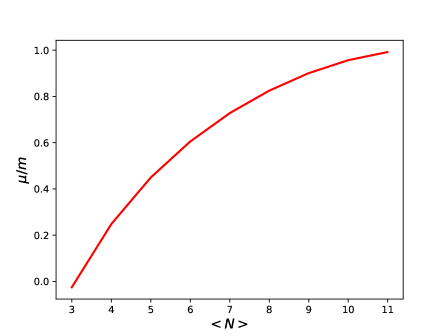
Figure 1: The $\mu/m$ dependence on $\langle N\rangle$. See the text for details.

Then, to calculate particle momentum spectra and correlations in the canonical ensembles, we need to evaluate $Z_{N}$ for various $N$. The results are plotted in Fig. 2.

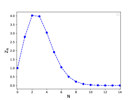
Figure 2: The $Z_{N}$ dependence on $N$. See the text for details.

Now, we are ready to compare spectra and correlations calculated in the grand-canonical and canonical ensembles. First, we compare particle number rapidity densities, $dN/dy$, for $\langle N\rangle=N$. As illustrated by Fig. 3, the grand-canonical particle number rapidity densities are virtually indistinguishable from their canonical counterparts.

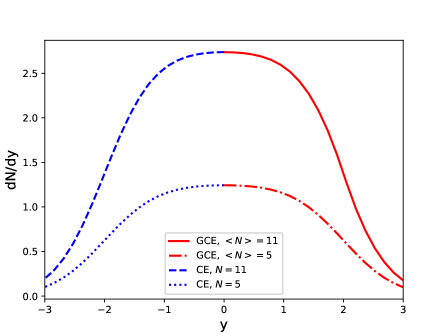
Figure 3: The particle rapidity densities for the canonical (left) and grand-canonical ensembles (right).

The transverse particle momentum spectra are compared in Fig. 4. Aside from the low transverse momenta region of the spectra with $N=\langle N\rangle=11$, where the grand-canonical spectrum is above the canonical one due to the Bose-Einstein enhancement ($\mu$ is approximately equal to $m$; see Fig. 1), we see no significant differences.

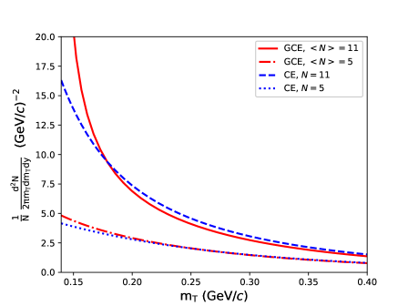
Figure 4: The transverse momentum spectra calculated in the canonical and grand-canonical ensembles with different $N=\langle N\rangle$.

Figures 5 and 6 display two-boson momentum correlation functions $C_{N}(\textbf{k}_{T},q_{L})$ calculated in the canonical ensembles as a function of the momentum difference. From these figures, it is evident that the intercepts of the canonical correlation functions, $C_{N}(\textbf{k}_{T},0)$, are not equal to $2$ and that the canonical correlation functions approach to $1$ from below when $|q_{L}|\rightarrow\infty$. It distinguishes two-boson correlation functions in the canonical ensembles from the ones in the corresponding grand-canonical ensembles where the correlation functions (not shown here) approach to $1$ from above and the intercepts are equal to $2$.

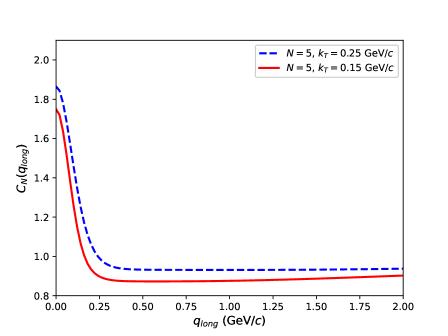
Figure 5: The canonical correlation functions for $N=5$ and several different values of $k_{T}$.

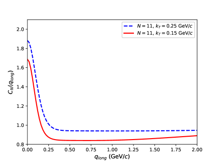
Figure 6: The canonical correlation functions for $N=11$ and several different values of $k_{T}$.

Notwithstanding the essential non-Gaussianity of the canonical correlation functions, if the fitting procedure is restricted to the correlation peak region, then the correlation function is well fitted by the Gaussian expression

$$C_{N}(\textbf{k}_{T},q_{L})=\frac{C_{N}(\textbf{k}_{T},0)}{2}\left(1+e^{-q_{L}^{2}R_{long}^{2}(k_{T},N)}\right).$$ (105)

It is instructive to compare canonical radius parameters extracted according to this expression with the ones calculated in the grand-canonical ensembles for $\langle N\rangle=N$,

$$C(\textbf{k}_{T},q_{L})=1+e^{-q_{L}^{2}R_{long}^{2}(k_{T},\langle N\rangle)}.$$ (106)

For definiteness, for both ensembles we apply the fitting procedures in the $q_{L}$ range $0<q_{L}<q_{L}^{max}$, where $q_{L}^{max}$ is such that $e^{-q_{L}^{2}R_{long}^{2}}=0.4$. Our results are depicted in Figs. 7 and 8. One can see that the canonical radius parameters slightly decrease with $N$, and the same trend, i.e., a decrease with $\langle N\rangle=N$, is also observed for the grand-canonical radius parameters that are slightly smaller than the canonical ones. This decrease with $\langle N\rangle=N$ can be interpreted as increasing deviations from the Boltzmann approximation. Figure 8 shows $R_{long}$ as a function on $k_{T}=|\textbf{k}_{T}|$ for several different values of $N$. One can see that $R_{long}$ in both ensembles is much smaller than the actual longitudinal size of the system ($\sim\tau\sinh{\eta_{f}}$) and decreases when $k_{T}$ increases. Such a smallness of the correlation radius parameters and a decline with increasing pair momentum are typical for locally equilibrated expanding systems Sin-1 . In Fig. 8 we plot for comparison the approximate analytical formula for $R_{long}$, $R_{long}\approx\tau\sqrt{\frac{1}{\beta m_{T}}}\sqrt{\frac{K_{2}(\beta m_{T})}{K_{1}(\beta m_{T})}}\approx\tau\sqrt{\frac{1}{\beta m_{T}}}\sqrt{1+\frac{3}{2\beta m_{T}}}$ Ber . The latter approximate equality is obtained by means of the asymptotic (large argument) expansion of the Macdonald functions. In the limit, $\beta m_{T}\gg 1$, this reduces to the formula $R_{long}\approx\tau\sqrt{\frac{1}{\beta m_{T}}}$ Sin-2 (see also Sin-3 ). All of the two figures reveal a consistent trend: if radius parameters are fitted in the region of the correlation peak, then deviations of the canonical radius parameters from their grand-canonical counterparts are rather small. It is also the case for $N=\langle N\rangle=11$ and small $k_{T}$, because the effects of the Bose-Einstein enhancement ($\mu$ is approximately equal to $m$ at $\langle N\rangle=11$) are nearly canceled out in the ratio (104).

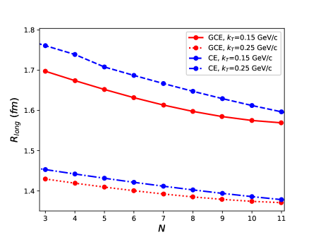
Figure 7: The $R_{long}$ dependence on $N=\langle N\rangle$ in the canonical and grand-canonical ensembles for several different values of $k_{T}$. See the text for details.

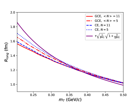
Figure 8: The $R_{long}$ dependence on $m_{T}$ in the canonical and grand-canonical ensembles for several different values of $N=\langle N\rangle$ and the $R_{long}$ calculated from the approximate analytic expression. See the text for details.

VI Conclusions

In this paper, we derived analytical expressions for one- and two- particle momentum spectra of a noninteracting relativistic boson field in the canonical ensemble described by the local-equilibrium statistical operator with a fixed particle number constraint. To see the effect of this constraint, we considered a corresponding grand-canonical state and compared the one-particle spectra and two-particle Bose-Einstein correlation functions. The correspondence was fixed by the condition that particle numbers, $N$, in the canonical states and mean particle numbers, $\langle N\rangle$, in the grand-canonical states are the same. Then, applying hydrodynamically motivated parametrization and parameter values that correspond roughly to the values at the system’s breakup in $p+p$ collisions at the LHC energies, we compare our results with the grand-canonical ensemble where artificial chemical potential, $\mu=\mbox{const}<m$, is taken such that $\langle N\rangle=N$. We have found that, calculated in both ensembles, one-particle momentum spectra are rather close to each other except for low transverse momenta region of the spectra with $N=\langle N\rangle=11$, where the grand-canonical spectrum is above the canonical one due to the Bose-Einstein enhancement ($\mu$ is approximately equal to $m$). Then, we compared the two-particle Bose-Einstein momentum correlations. We demonstrated that there are small quantitative but qualitative differences between the correlation radius parameters in both ensembles if they are fitted in the region of the correlation peak: the canonical radius parameters are slightly larger than the grand-canonical ones. Furthermore, we showed that, in contrast to the predictions of the grand-canonical ensemble, the intercepts of the canonical correlation functions are not equal to $2$ and depend on particle multiplicities and momenta and that the canonical correlation functions can be less than unity in some intermediate region of relative momentum of particles. Such features should be taken into account when theoretical models are compared with the multiplicity-dependent measurements of the Bose-Einstein momentum correlations. As a final comment, we wish to note that the apparent independence of correlation radius parameters on the particle number densities in high-multiplicity $p+p$ collisions at a fixed energy of the LHC Atlas ; CMS still remains unexplained, inviting further studies.

References

• (1) M. Gyulassy, S.K. Kauffmann, and L.W. Wilson, Phys. Rev. C 20, 2267 (1979); M.I. Podgoretsky, Fiz. Elem. Chast. At. Yad. 20, 628 (1989) [Sov. J. Part. Nucl. 20, 266 (1989)]; D.H. Boal, C.-K. Gelbke, B.K. Jennings, Rev. Mod. Phys. 62, 553 (1990); U.A. Wiedemann, U. Heinz, Phys. Rep. 319, 145 (1999); R.M. Weiner, Phys. Rep. 327, 249 (2000); R.M. Weiner, Introduction to Bose-Einstein Correlations and Subatomic Interferometry (Wiley, New York, 2000); M. Lisa, S. Pratt, R. Soltz, U. Wiedemann, Annu. Rev. Nucl. Part. Sci. 55, 357 (2005); R. Lednický, Phys. Part. Nucl. 40, 307 (2009); Yu.M. Sinyukov, V.M. Shapoval, Phys. Rev. D 87, 094024 (2013).
• (2) J. Adam et al. (ALICE Collaboration), Phys. Rev. C93, 024905 (2016).
• (3) ATLAS Collaboration, Eur. Phys. J. C 75, 466 (2015); 82, 608 (2022).
• (4) A.M. Sirunyan et al. (CMS Collaboration), Phys. Rev. C 97, 064912 (2018); J. High Energy Phys. 03 (2020) 014.
• (5) L. McLerran, M. Praszalowicz, B. Schenke, Nucl. Phys. A916, 210 (2013).
• (6) B. Schenke, Rep. Prog. Phys. 84, 082301 (2021).
• (7) D.N. Zubarev, Nonequilibrium Statistical Thermodynamics (Plenum Press, New York, 1974); A. Hosoya, M. Sakagami and M. Takao, Ann. Phys. (N.Y.) 154, 229 (1984); D. Zubarev, V. Morozov, G. Röpke, Statistical Mechanics of Nonequilibrium Processes. Volume 1: Basic Concepts. Kinetic Theory (Akademie Verlag, Berlin, 1996); Statistical Mechanics of Nonequilibrium Processes. Volume 2: Relaxation and Hydrodynamic Processes (Akademie Verlag, Berlin, 1997); F. Becattini, L. Bucciantini, E. Grossi, and L. Tinti, Eur. Phys. J. C 75, 191 (2015); F. Becattini, M. Buzzegoli, and E. Grossi, Particles 2, 197 (2019); A. Harutyunyan, A. Sedrakian, D.H. Rischke, Ann. Phys. (Amsterdam) 438, 168755 (2022).
• (8) S.V. Akkelin, Yu. M. Sinyukov, Phys. Rev. C 94, 014908 (2016).
• (9) M.D. Adzhymambetov, S.V. Akkelin, Yu.M. Sinyukov, Phys. Rev. D 103, 116012 (2021); 105, 096035 (2022).
• (10) M. Gaudin, Nucl. Phys. 15, 89 (1960).
• (11) S.R. de Groot, W.A. van Leeuwen, and Ch.G. van Weert, Relativistic Kinetic Theory (North-Holland, Amsterdam, 1980).
• (12) N. Dowling, S. Floerchinger, T. Haas, Phys. Rev. D 102, 105002 (2020).
• (13) C. Bloch and C. De Dominicis, Nucl. Phys. 7, 459 (1958).
• (14) J.D. Bjorken, Phys. Rev. D 27, 140 (1983).
• (15) M. Herrmann, G.F. Bertsch, Phys. Rev. C 51, 328 (1995).
• (16) A.N. Makhlin, Yu.M. Sinyukov, Z. Phys. C 39, 69 (1988); Yu.M. Sinyukov, Nucl. Phys. A498, 151c (1989).
• (17) Yu.M. Sinyukov, S.V. Akkelin, A.Yu. Tolstykh, Nucl. Phys. A610, 278c (1996).