Text-CRS: A Generalized Certified Robustness Framework against Textual Adversarial Attacks

Abstract

The language models, especially the basic text classification models, have been shown to be susceptible to textual adversarial attacks such as synonym substitution and word insertion attacks. To defend against such attacks, a growing body of research has been devoted to improving the model robustness. However, providing provable robustness guarantees instead of empirical robustness is still widely unexplored. In this paper, we propose Text-CRS, a generalized certified robustness framework for natural language processing (NLP) based on randomized smoothing. To our best knowledge, existing certified schemes for NLP can only certify the robustness against $\ell_{0}$ perturbations in synonym substitution attacks. Representing each word-level adversarial operation (i.e., synonym substitution, word reordering, insertion, and deletion) as a combination of permutation and embedding transformation, we propose novel smoothing theorems to derive robustness bounds in both permutation and embedding space against such adversarial operations. To further improve certified accuracy and radius, we consider the numerical relationships between discrete words and select proper noise distributions for the randomized smoothing. Finally, we conduct substantial experiments on multiple language models and datasets. Text-CRS can address all four different word-level adversarial operations and achieve a significant accuracy improvement. We also provide the first benchmark on certified accuracy and radius of four word-level operations, besides outperforming the state-of-the-art certification against synonym substitution attacks.

1 Introduction

With recent advances in natural language processing (NLP), large language models (e.g., ChatGPT [1] and Chatbots [2, 3, 4]) have become increasingly popular and widely deployed in practice. Wherein, text classification plays an important role in language models, and it has a wide range of applications, including content moderation, sentiment analysis, fraud detection, and spam filtering [5, 6]. Nevertheless, text classification models are vulnerable to word-level adversarial attacks, which imperceptibly manipulate the words in input text to alter the output [7, 8, 9, 10, 11, 12, 13]. These attacks can be exploited maliciously to spread misinformation, promote hate speech, and circumvent content moderation [14].

To defend against such attacks, numerous techniques have been proposed to improve the robustness of language models, especially for text classification models. For instance, adversarial training  [15, 16, 17] retains the model using both clean and adversarial examples to enhance the model performance; feature detection [18, 19] checks and discards detected adversarial inputs to mitigate the attack; and input transformation [20, 21] processes the input text to eliminate possible perturbations. However, these empirical defenses are only effective against specific adversarial attacks and can be broken by adaptive attacks [9].

One promising way to win the arms race against unseen or adaptive attacks is to provide provable robustness guarantees for the model. This line of work aims to develop certifiably robust algorithms that ensure the model’s predictions are stable over a certain range of adversarial perturbations. Among different certified defense methods, randomized smoothing [22, 23, 24] does not impose any restrictions on the model architecture and achieves acceptable accuracy for large-scale datasets. This method injects random noise, sampled from a smoothing distribution, into the input data during training to smoothen the classifier. The smoothed classifier will make a consistent prediction for a perturbed test instance (with noise) as the original class label. Despite the successful application of randomized smoothing in protecting vision models, applying these methods to safeguard language models remains fairly challenging.

Table I: Comparison of certified defense methods for NLP robustness against textual adversarial attacks.

Method	Model architecture	Adversarial operations (smoothing distribution / $\ell_{p}$ perturbation)				Certified	Uni-	Accuracy
		Substitution	Reordering	Insertion	Deletion	radius / $\mathtt{RAD}$	versality	(large-scale data)
IBP-trained [25]	LSTM/Att. layer	✓	✓	✓	✓	✗	✗	Low
POPQORN [26]	RNN/LSTM/GRU	✓	✓	✓	✓	✗	✗	Low
Cert-RNN [27]	RNN/LSTM	✓	✓	✓	✓	✗	✗	Low
DeepT [28]	Transformer	✓	✓	✓	✓	✗	✗	Low
SAFER [29]	Unrestricted	✓ (Uniform / $\ell_{0}$)	✗	✗	✗	✓ Practical	✗	High
RanMASK [30]	Unrestricted	✓ (Uniform / $\ell_{0}$)	✗	✗	✗	✓	✗	High
CISS [31]	Unrestricted	✓ (Gaussian / $\ell_{2}$)	✗	✗	✗	✓	✗	High
Text-CRS (Ours)	Unrestricted	✓ (Staircase / $\ell_{1}$)	✓ (Uniform / $\ell_{1}$)	✓ (Gaussian / $\ell_{2}$)	✓ (Bernoulli / $\ell_{0}$)	✓ Practical	✓	$>$ SOTA

• 1. The model architectures applicable to the first four methods have size restrictions, i.e., the number and size of layers cannot be too large.

• 2. ”Practical” means that the certified radius can correspond to the $\mathtt{RAD}$-word level of perturbation. (We propose four practical certified radii.)

First, due to the discrete nature of the text data, numerical $\ell_{1}$ or $\ell_{2}$-norms cannot be directly used to measure the distance between texts. Without considering word embeddings, previously certified defenses in the NLP domain, such as SAFER [29] and WordDP [32], are limited to certifying robustness against $\ell_{0}$ perturbations generated by synonym substitution attacks. Also, their assumption of uniformly distributed synonyms is impractical, leading to relatively low certified accuracy. Second, text classification models are vulnerable to a range of word-level operations that result in various perturbations. For instance, the word insertion operation introduces random words in the lexicon, while the word reordering operation causes positional permutation. These diverse perturbations can deceive text classification models successfully [10, 9, 11, 12, 13]. To our best knowledge, there exist no certified defense methods against these word-level perturbations. Third, significant absolute differences between adversarial and clean texts may exist due to word-level operations, while conventional randomized smoothing can only ensure the model’s robustness against perturbations within a small radius. Prior works [33, 34, 35, 36, 37] for images address this challenge by providing robustness guarantees against semantic transformations (e.g., rotation, scaling, shearing). However, they cannot be directly applied to the NLP domain because texts and words have a more heterogeneous discrete domain, and word insertion and deletion are new semantic transformations not involved in the image domain.

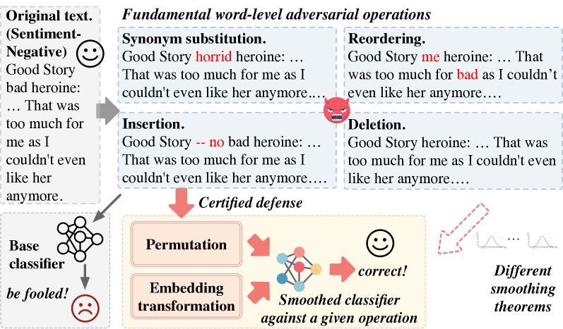
Figure 1: Text-CRS is a robustness certification framework based on randomized smoothing of permutation and embedding transformations against word-level adversarial attacks.

In this paper, we present Text-CRS, the first generalized certified robustness framework against common word-level textual adversarial attacks (i.e., synonym substitutions, reorderings, insertions, and deletions) via randomized smoothing (see Figure 1). Text-CRS certifies the robustness in the word embedding space without imposing restrictions on model architectures, and demonstrates high universality and superior accuracy compared to state-of-the-art (SOTA) methods (see Table I). Specifically, we first model all the word-level adversarial attacks as combinations of permutations and embedding transformations. For instance, synonym substitution attacks transform the original words’ embedding vectors with the synonyms’ embedding vectors, while word recordering attacks transform the word orderings with certain word permutations. Then, the word-level adversarial attacks can be guaranteed to be certified robust (“practical”) when their corresponding permutation and embedding transformation are certified.

To this end, we develop customized theorems (see Section 4) to derive the certified robustness against each attack. In each theorem, we use an appropriate noise distribution for our smoothing distributions in order to fit different word-level attacks. For instance, unlike existing works [29, 38] that use the uniform distribution, we propose to use the Staircase-shape distribution [39] to simulate the synonym substitutions, which ensures that semantically similar synonyms are more likely to be substituted. Moreover, we use a uniform distribution to simulate the word reordering. For the word insertion with a wide range of inserted words, we inject Gaussian noise into the embeddings. For the word deletion, the embedding vector of each word is either kept or deleted (i.e., set to be zero). Hence, we use the Bernoulli distribution to simulate the status of each word. Our certified radii for the four attacks are then derived based on the corresponding noise distributions.

To further improve the certified accuracy/radius, we also propose a training toolkit incorporating three optimization techniques designed for training. For instance, instead of using isotropic Gaussian noises that can lead to distortion in the word embedding space, we propose to use an anisotropic Gaussian noise and optimize it to enlarge the certified radius.

Thus, our major contributions are summarized below:

• To our best knowledge, we propose the first generalized framework Text-CRS to certify the robustness for text classification models against four fundamental word-level adversarial operations, covering most word-level textual adversarial attacks. Also, the certification against word insertion can be universally applied to other operations.

• We provide novel robustness theorems based on Staircase, Uniform, Gaussian, and Bernoulli smoothing distributions against different operations. We also theoretically derive certified robustness bounds for each operation.

• To study the deceptive potential of adversarial texts, we apply ChatGPT to assess whether adversarial texts can be crafted to be semantically similar to clean texts.

• We conduct extensive experiments to evaluate Text-CRS, including our enhanced training toolkit, on three real datasets (AG’s News, Amazon Review, and IMDB) with two NLP models (LSTM and BERT). The results show that Text-CRS effectively handles five representative adversarial attacks and achieves an average certified accuracy of $81.7\%$, which is a $64\%$ improvement over the SOTA methods. Text-CRS also significantly outperforms the SOTA methods on the substitution operation. Besides, it provides new benchmarks for certified robustness against the other three operations.

2 Preliminaries

2.1 Text Classification

The objective of text classification is to map texts to labels. A text consisting of $m$ words is denoted as $x=\{x_{1},...,x_{m}\}$, where $x_{i}$ is the $i$th word, aka., a token. Text classification involves three key components: data processing, embedding layer, and classification model. Given a text $x$ labeled $y$, data processing first pads it to a fixed length $n$. When $m<n$, the processing inserts $n-m$ <pad> tokens to the end of the text, and when $m>n$, the processing drops the $m-n$ tokens. For brevity, we will denote a text $x$ with a fixed length of $n$ after data processing, i.e., $x=\{x_{1},...,x_{n}\}$. Then, the embedding layer converts each token $x_{i}$ into a high-dimensional embedding vector $w_{i}$. After deriving the embedding matrix $w=\{w_{1},\cdots,w_{n}\}$, the text classification model $h$ learns the relationship between the embedding matrix $w$ and the label $y$. For a tuple $(w,y)$, the model uses a loss function $\ell$ to derive the loss $\ell(h(w),y)$ and updates the model $h$, e.g., using stochastic gradient descent.

In text classification tasks, the embedding layer is essential for representing words in a text and often has a large number of parameters. In practice, the embedding layer is usually a pre-trained word embedding, such as Glove [40] or a pre-trained language model, such as BERT [41]. The parameters in the embedding layer are frozen and only parameters in the classification model are updated during training. The classification model typically uses a deep neural network of different architectures, such as recurrent neural network (RNN) [42], convolutional neural network (CNN) [43], and Transformer model [44].

2.2 Adversarial Examples for Text Classification

Adversarial examples are well-crafted inputs that lead to the misclassification of machine learning models via slightly perturbing the clean data. In text classification, an adversarial text fools the text classification model, and is also semantically similar to the clean text for human imperceptibility. To generate adversarial texts, there are three main approaches based on different perturbation strategies. (1) Character-level adversarial attacks [45, 46, 47] substitute, swap, insert, or delete certain characters in a word and generate carefully crafted typos, such as changing “terrible” to “terrib1e”. However, these typos can be detected and corrected by spell checker easily [48]. (2) Word-level adversarial attacks [9, 49, 50, 10, 13] alter the words within a text through four primary operations: substituting words with their synonyms, reordering words, inserting descriptive words, and deleting unimportant words. This attack is widely exploited because only a few words of perturbations can lead to a high attack success rate [51]. (3) Sentence-level adversarial attacks [52, 53] adopt another perturbation strategy that paraphrases the whole sentence or inserts irrelevant sentences into the text. This approach affects predictions by disrupting the syntactic and logical structure of sentences rather than specific words. However, this attack makes it difficult to preserve the original semantics due to rephrasing or inserting irrelevant sentences [21].

As discussed above, the word-level adversarial attacks have widespread and severe impacts. Thus, in this paper, we focus on the certified defenses against word-level adversarial attacks. We distill and consolidate such attacks into four fundamental adversarial operations: substitution, reordering, insertion, and deletion (see Figure 1). We offer provable robustness guarantees against these operations. The proposed theorems and defense methods can be extended to the other two types of adversarial attacks on text classification with the similar operations.

Synonym Substitution: this operation generates adversarial texts by replacing certain words in the text with their synonyms, thereby preserving the text’s semantic meanings. For instance, to minimize the word substitution rate, TextFooler [9] picks the word crucial to the prediction, i.e., when this word is removed, the prediction undergoes a significant deviation; then, it selects synonyms with high cosine similarity to the original embedding vector for substitution.

Word Reordering: this operation selects and randomly reorders several consecutive words in the text while keeping the words themselves unchanged. For instance, WordReorder [49] investigates the sensitivity of NLP systems to such adversarial operation and shows that reordering leads to an average decrease in the accuracy of 18.3% and 15.4% for the LSTM-based model and BERT on five datasets.

Word Insertion: this operation generates adversarial text by inserting new words into the clean text. For instance, the NLP adversarial example generation library TextAttack [50] includes a basic insertion strategy SynonymInsert that inserts synonyms of words already in the text to maintain semantic similarity between adversarial and clean texts. BAE-Insert [10] uses masked language models (e.g., BERT) to predict newly inserted <mask> tokens in the text. The predicted words are then used to replace the <mask> tokens for the adversarial text. Compared to SynonymInsert, BAE-Insert improves syntactic and semantic consistency.

Word Deletion: this operation generates adversarial texts by removing several words from clean text. InputReduction [13] iteratively removes the least significant words from the clean text, and demonstrates that specific keywords play a critical role in the prediction of language models. Table X shows that it can lead to an average of $51.78\%$ accuracy reduction.

2.3 Threat Model

We consider a threat model similar to that of other randomized smoothing and certified methods [29, 31, 34], which guarantees robustness as long as perturbations remain within the certified radius. They provide effective defense against both white-box and black-box attacks, irrespective of the specific attack types and adopted methods. Specifically, we assume that the adversary can launch the evasion attack on a given text classification model by intercepting the input and perturbing the input with a wide variety of word-level adversarial attacks [9, 49, 50, 10]. Given a text classification model $h$ and a text $x$ with label $y$, the goal of the adversary is to craft an adversarial text $x^{\prime}$ from $x$ to alter its prediction, i.e., $h(x^{\prime})\neq h(x)=y$. While generating the adversarial texts, the adversary can choose any single aforementioned word-level adversarial operation or a combination thereof, as all textual adversarial attacks can be unified as the transformation of the embedding vector. These four types of operations encompass almost all possible modifications to texts in adversarial attacks [49] and their formal definitions are provided as below:

Synonym Substitution: we replace certain words in the text $x$ with synonyms of the original word. Specifically, we convert each word $x_{i}$ to $x_{i}^{\prime}$, where $x_{i}^{\prime}$ may be a synonym of $x_{i}$ or $x_{i}$ itself. The operation can be represented as:

$$x=\{{x_{1}},\cdots,{x_{n}}\}\to x^{\prime}=\{x_{1}^{\prime},\cdots,x_{n}^{\prime}\},$$

where $x$ and $x^{\prime}$ are of the same length.

Word Reordering: to reorder certain words in the text $x$, we move the word at position $i$ to position $r_{i}$, where $r_{i}$ may be equal to $i$. The operation can be expressed as:

$$x=\{{x_{1}},\cdots,{x_{n}}\}\to x^{\prime}=\{{x_{r_{1}}},\cdots,{x_{r_{n}}}\},$$

where $x$ and $x^{\prime}$ are of the same length.

Word Insertion: we insert a word $x_{\mathrm{In}}^{1}$ into the $j_{1}$th position, a word $x_{\mathrm{In}}^{2}$ into the $j_{2}$th position, $\cdots$, and a word $x_{\mathrm{In}}^{m^{\prime}}$ into the $j_{m^{\prime}}$th position to $x$, where $m^{\prime}$ is the total number of inserted words. The operation can be expressed as:

$$x= \{x_{1},\cdots,x_{j_{1}-1},x_{j_{1}},\cdots,x_{j_{2}-1},x_{j_{2}},\cdots,x_{n}\}\to$$

$$x^{\prime}= \{x_{1},\cdots,x_{j_{1}-1},x_{\mathrm{In}}^{1},x_{j_{1}},\cdots,x_{j_{2}-1},x_{\mathrm{In}}^{2},x_{j_{2}},\cdots,x_{n}\},$$

where $x^{\prime}$ includes $m^{\prime}$ more words than $x$.

Word Deletion: we delete $m^{\prime}$ words at position $j_{1},\cdots,j_{m^{\prime}}$ from $x$. The operation can be represented as:

$$x= \{x_{1},\cdots,x_{j_{1}-1},x_{j_{1}},x_{j_{1}+1},\cdots,x_{j_{2}-1},x_{j_{2}},\cdots,x_{n}\}\to$$

$$x^{\prime}= \{x_{1},\cdots,x_{j_{1}-1},x_{j_{1}+1},\cdots,x_{j_{2}-1},x_{j_{2}+1},\cdots,x_{n}\},$$

where $x^{\prime}$ includes $m^{\prime}$ words less than $x$.

2.4 Randomized Smoothing for Certified Defense

Randomized smoothing [54, 22] is a widely adopted certified defense method that offers state-of-the-art provable robustness guarantees for classifiers against adversarial examples. It has two key advantages: applicable to any classifier and scalable to large models. Given a testing example ${x}$ with label $y$ from a label set $\mathcal{Y}$, randomized smoothing has three steps: 1) define a (base) classifier $h$; 2) build a smoothed classifier $g$ based on $h$, ${x}$, and a noise distribution; and 3) derive certified robustness for the smoothed classifier $g$. Under our context, the base classifier $h$ can be any trained text classifier and $x$ is a testing text. Let $\epsilon$ be a random noise drawn from an application-dependent noise distribution. Then the smoothed classifier $g$ is defined as $g({x})=\operatorname*{arg\,max}_{l\in\mathcal{Y}}\text{Pr}(h({x}+\epsilon)=l)$. Let $p_{A},p_{B}\in[0,1]$ be the probability of the most ($y_{A}$) and the second most probable class ($y_{B}$) outputted by $\text{Pr}(h({x}+\epsilon))$, respectively, i.e., $p_{A}=\max_{l}\text{Pr}(h({x}+\epsilon)=l)$ and $p_{B}=\max_{l\neq y_{A}}\text{Pr}(h({x}+\epsilon)=l)$. Then $g$ provably predicts the same label $y_{A}$ for ${x}$ once the adversarial perturbation $\delta$ is bounded, i.e., $g({x}+\delta)=y_{A},\forall||\delta||_{p}\leq R$, where $||\cdot||_{p}$ is an $\ell_{p}$ norm and $R$ is called certified radius that depends on $p_{A},p_{B}$. For example, when the noise distribution is an isotropic Gaussian distribution with mean 0 and standard deviation $\sigma$, [22] adopted the Neyman-Person Lemma [55] and derived a tight robustness guarantee against $l_{2}$ perturbation, i.e., $g({x}+\delta)=y_{A},\forall||\delta||_{2}\leq R=\frac{\sigma}{2}(\Phi^{-1}({p_{A}})-\Phi^{-1}({p_{B}}))$, where $\Phi^{-1}$ is the inverse of the standard Gaussian CDF. This property implies that the smoothed classifier $g$ maintains constant predictions if the norm of the perturbation $\delta$ is smaller than the certified radius $R$.

3 The Text-CRS Framework

This section introduces Text-CRS, a novel certification framework that offers provable robustness against adversarial word-level operations. We first outline the new challenges in designing such certified robustness. Next, we formally define the permutation and embedding transformations that correspond to each adversarial operation. We then define the perturbation that Text-CRS can certify for each permutation and embedding transformation. Finally, we conclude with a summary of our framework and its defense goals.

3.1 New Challenges in Certified Defense Design

Previous studies on certified defenses in text classification, including SAFER [29] and CISS [31], only provide robustness guarantees against substitution operations. Certified defenses against other word-level operations, such as word reordering, insertion, and deletion, are unexplored. We list below the weaknesses of existing defenses as well as several technical challenges:

• Measuring the perturbation and certified radius. Words are unstructured strings and there is no numerical relationship among discrete words. This makes it challenging to measure the $\ell_{1}$ and $\ell_{2}$ distance between words, as well as the perturbation distance between the original and adversarial text (while deriving the certified radius).

• Customized noise distribution for randomized smoothing against different word-level attacks. The assumption of a uniform substitution distribution among synonyms is unrealistic, as different synonyms exhibit varying substitution probabilities. However, previous works on the certified robustness against word substitution almost assume a uniform distribution within the set of synonyms. Such an assumption makes these works yield relatively low certified accuracy (see Section 6.2). Hence, we need to construct customized noise distributions best suited for the certification against the synonyms substitution attack as well as the other three word-level attacks.

• Inaccurate representation of distance. The absolute distance between operation sequences is typically high for word reordering, insertion, and deletion operations. Although studies, such as TSS [34] and DeformRS [35], have investigated the pixel coordinate transformation in the image domain, the word reordering transformation has not been studied in the NLP domain. Moreover, word insertion and deletion are unique transformations specific to NLP which are not applicable in the image domain.

To address these challenges, we employ the numerical word embedding matrix[40, 41] as inputs to our model instead of the word sequence. We can then use embedding matrices to measure the $\ell_{1}$ and $\ell_{2}$ distance between word sequences. We also introduce a permutation space to solve the problem of high absolute distance. Moreover, we design a customized noise distribution for randomized smoothing w.r.t. each attack and derive the corresponding certified radius, shown in Theorems in Section 4.

3.2 Permutation and Embedding Transformation

Table II: Frequently Used Notations

Term	Description
$\mathcal{X}$	Input text space
$\mathcal{W}\subseteq\mathbb{R}^{n\times d}$	Embedding space
$\mathcal{U}\subseteq\mathbb{R}^{n\times n}$	Permutation space
$\mathcal{U}\cdot\mathcal{W}\subseteq\mathbb{R}^{n\times d}$	Embedding space after applying permutation
$\mathcal{Y}$	Label space
$\theta(u,r):\mathcal{U}\times\mathcal{R}$	Permutation with parameter $r$ on $u$
$\phi(w,t):\mathcal{W}\times\mathcal{T}$	Embedding transformation with parameter $t$ on $w$
$L_{emb}:\mathcal{X}\to\mathcal{W}$	The pre-trained embedding layer
$h:\mathcal{U}\cdot\mathcal{W}\to\mathcal{Y}$	Classification model (i.e., base classifier)
$n$	Constant maximum length of input sequence
$d$	Dimension of each embedding vector
$\delta$	Perturbations of permutation or embedding space

3.2.1 Notations

We denote the space of input text as $\mathcal{X}$, the space of corresponding embedding as $\mathcal{W}\subseteq\mathbb{R}^{n\times d}$ (where $n$ is the constant maximum length of each input sequence and $d$ is the dimension of each embedding vector), and the space of output as $\mathcal{Y}=\{1,\cdots C\}$ where $C$ is the number of classes. We denote the space of embedding permutations as $\mathcal{U}\subseteq\mathbb{R}^{n\times n}$. For instance, given a word sequence $x$, its embedding matrix is $w=\{w_{1},\cdots,w_{n}\}$, its permutation matrix is $u=\{u_{1},\cdots,u_{n}\}$, and the input to the classification model will be $u\cdot w$. The position of $w_{i}$ is denoted by $u_{i}=[0,\cdots,0,1,0,\cdots,0]$, a standard basis vector represented as a row vector of length $n$ with a value of $1$ in the $i$th position and a value of $0$ in all other positions.

We model the permutation transformation as a deterministic function $\theta:\mathcal{U}\times\mathcal{R}\to\mathcal{U}$, where the permutation matrix $u\in\mathcal{U}$ is permuted by a $\mathcal{R}$-valued parameter $r$. Vector $u_{i}$ is replaced with $u_{r}$ by applying $r$, and then the word embedding ($w_{i}$) is moved from position $i$ to $r$. Moreover, we model the embedding transformation as a deterministic function $\phi:\mathcal{W}\times\mathcal{T}\to\mathcal{W}$, where the original embedding $w\in\mathcal{W}$ is transformed by a $\mathcal{T}$-valued parameter $t$. Based on such transformation, we can define all the operations in Section 2.3. For example, $\theta_{I}(u,r)\cdot\phi_{I}(w,t)$ represents the word insertion on the original input $u\cdot w$ with a permutation parameter $r$ and an embedding parameter $t$. Here, we denote $\cdot$ as applying the permutation $u$ to the embedding $w$, and $\times$ as the operations of the parameters applied to the permutation or the embedding matrices.

For simplicity of notations, we denote the classification model as $h:\mathcal{U}\cdot\mathcal{W}\to\mathcal{Y}$. Then, we adopt the pre-trained embedding layer ($L_{emb}$) for the text classification task, freeze its parameters, and only update parameters in the classification model. Essentially, the input space of the model ($\mathcal{U}\cdot\mathcal{W}\subseteq\mathbb{R}^{n\times d}$) is the same as $\mathcal{W}$, and the training process of $h$ is identical to that of a classical text classification model. Table II shows our frequently used notations.

3.2.2 Permutation and Embedding Transformation

Given the above permutation and embedding transformations, synonym substitution and word reordering are single transformations while word insertion and deletion are composite transformations. Our transformations of the input tuple $(u=\{u_{1},\cdots,u_{n}\},w=\{w_{1},\cdots,w_{n}\})$ are further represented as follows (no change to the sizes of $u$ and $w$).

Synonym Substitution replaces the original word’s embedding vector with the synonym’s embedding vector.

$$(\theta_{S}(u,\textrm{null}),\phi_{S}(w, \{a_{1},\cdots,a_{n}\}))$$

$$\qquad=(u,{w^{\prime}})= (u,\{w_{1}^{a_{1}},\cdots,w_{n}^{a_{n}}\})$$

where $w_{j}^{a_{j}}$ ($a_{j}$ are nonnegative integers) is the embedding vector of the $a_{j}$th synonym of the original embedding $w_{j}$, and $a_{j}=0$ indicates $w_{j}$ itself: $w_{i}^{0}=w_{i}$. The permutation $\theta_{S}(u,\textrm{null})$ does not modify any entries of the permutation matrix $u$.

Word Reordering does not modify the embedding vector but modifies the permutation matrix.

$$(\theta_{R}(u,\{r_{1},\cdots,r_{n}\}), \ \phi_{R}(w,\textrm{null}))$$

$$\qquad=(u^{\prime},{w})= (\{{u_{r_{1}}},\cdots,{u_{r_{n}}}\},w)$$

where $\{r_{1},\cdots,r_{n}\}$ is the reordered list of $\{1,\cdots,n\}$. The transformation $\phi_{R}(w,\textrm{null})$ does not modify the elements of the embedding matrix $w$.

Word Insertion first inserts $m^{\prime}$ embedding vectors of the specified words at the specified positions ($j_{1},\cdots,j_{m^{\prime}}$). Then, it removes the last $m^{\prime}$ embedding vectors to maintain the constant length $n$ of the text. (see Figure 2)

$$(\theta_{I}(u,\{r_{1},\cdots,r_{n}\})),\phi_{I}(w,\{w_{\mathrm{In}}^{1},\cdots,w_{\mathrm{In}}^{m^{\prime}}\}))$$

$$= (u^{\prime}_{0},w^{\prime}_{0})=\!(\{u_{1},\cdots,u_{j_{1}-1},u_{j_{1}},u_{j_{1}+1},\cdots,u_{n}\},$$

$$\qquad\quad\{w_{1},\cdots,w_{j_{1}-1},w_{\mathrm{In}}^{1},w_{j_{1}},\cdots,w_{n-m^{\prime}}\})$$

$$= (u^{\prime},w^{\prime})=\!(\{u_{1},\cdots,u_{j_{1}-1},u_{j_{1}+1},\cdots,u_{n},u_{j_{1}},\cdots u_{j_{m^{\prime}}}\},$$

$$\qquad\quad\{w_{1},\cdots,w_{j_{1}-1},w_{j_{1}},\cdots,w_{n-m^{\prime}},w_{\mathrm{In}}^{1},\cdots,w_{\mathrm{In}}^{m^{\prime}}\})$$

where $w_{\mathrm{In}}^{i}$ is the embedding vector of the inserted word at position $j_{i}$, $i\in[1,m^{\prime}]$. To minimize the distance between $w$ and $w^{\prime}_{0}$, $w_{\mathrm{In}}^{i}$ and its corresponding position vector $u_{j_{i}}$ are shifted to the end of the sequence to obtain $(u^{\prime},w^{\prime})$.

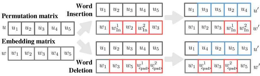
Figure 2: Word insertion and deletion. Blue and red indicate the changes to the permutation and embedding matrices.

Word Deletion first replaces $m^{\prime}$ embedding vectors with all-zero vectors (of <pad>) at position $j_{1},\cdots,j_{m^{\prime}}$. Then it moves the positions (i.e., permutation vector) of these all-zero vectors to the end of the sequence. (see Figure 2)

$$(\theta_{D}(u,\{r_{1},\cdots,r_{n}\})),\phi_{D}(w,\{j_{1},\cdots,j_{m^{\prime}}\}))$$

$$= (u^{\prime},w^{\prime})=(\{u_{1},\cdots,u_{j_{1}-1},{u_{n-m^{\prime}+1}},u_{j_{1}},\cdots,u_{n-m^{\prime}}\},$$

$$\qquad\qquad\quad\{w_{1},\cdots,w_{j_{1}-1},{w_{\texttt{<pad>}}^{1}},w_{j_{1}+1},\cdots,w_{n}\})$$

where $w_{\texttt{<pad>}}^{i}$ is the embedding vector of <pad> (i.e., the all-zero vector), and it replaces the original embedding vector $w_{j_{i}}$, $i\in[1,m^{\prime}]$. The position vector of $w_{\texttt{<pad>}}^{i}$ is $u_{n-m^{\prime}+i}$, such that $u^{\prime}\cdot w^{\prime}$ corresponds to the embedding matrix generated after deleting $m^{\prime}$ words at position $j_{1},\cdots,j_{m^{\prime}}$ in the text $x$.

3.3 Framework Overview

3.3.1 Perturbations of Adversarial Operations

Since different operations involve different permutations and embedding transformations, we first define their perturbations and will certify against these perturbations in Section  4.

Synonym Substitution involves only the embedding substitution, which can be represented as $w\oplus\delta_{S}=\{w_{1}\oplus a_{1},\cdots,w_{n}\oplus a_{n}\}$. Here, $w_{j}\oplus a_{j}$ denotes the replacement of the word embedding $w_{j}$ with any of its synonyms $w_{j}^{a_{j}}$, while the original embedding can be $w_{j}=w_{j}\oplus 0$. Thus, the perturbation is defined as $\delta_{S}=\{a_{1},\cdots,a_{n}\}$.

Word Reordering involves only the permutation of embeddings, which can be represented as $u\oplus\delta_{R}=\{u_{1}\oplus r_{1},\cdots,u_{n}\oplus r_{n}\}$, where $u_{j}\oplus r_{j}=u_{r_{j}}$ indicates that the embedding originally at position $j$ is reordered to position $r_{j}$. The reordering perturbation is $\delta_{R}=\{r_{1}-1,\cdots,r_{n}-n\}$.

Word Insertion includes permutation and embedding insertion, with the permutation perturbation, $\delta_{R}$, being identical to word reordering. Embedding insertion preserves the first $n-m^{\prime}$ embeddings while replacing only the last $m^{\prime}$ embeddings with new ones. The perturbation of insertion is defined as $\delta_{I}=\{w_{\mathrm{In}}^{1}-w_{n-m^{\prime}+1},\cdots,w_{\mathrm{In}}^{m^{\prime}}-w_{n}\}$.

Word Deletion involves permutation and embedding deletion, where permutation perturbation is equivalent to $\delta_{R}$. We model the embedding deletion that converts any selected embedding to $w_{\texttt{<pad>}}$ as an embedding state transition from $b=1$ to $b=0$. The deletion perturbation is therefore defined as $\delta_{D}=\{1-b_{1},\cdots,1-b_{n}\}$, where all $b_{j},j\in[1,n]$ are equal to 1, except for $b_{j_{1}}=0,\cdots,b_{j_{m^{\prime}}}=0$, which represents the deleted embeddings at positions $j_{1},\cdots,j_{m^{\prime}}$.

3.3.2 Framework and Defense Goals

Figure 3 summarizes our Text-CRS framework. The input space is partitioned into a permutation space $\mathcal{U}$ and an embedding space $\mathcal{W}$, by representing each operation as a combination of permutation and embedding transformation (see Section 3.2.2). We analyze the characteristics of each operation and select an appropriate smoothing distribution to ensure certified robustness for each of them (see Section 4).

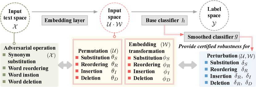
Figure 3: An overview of Text-CRS.

Since each word-level operation is equivalent to a combination of the permutation and embedding transformation, any adversary perturbs the text input is indeed adjusting the parameter tuple $(r,t)$ of permutation and embedding transformation. Our goal is to guarantee the robustness of the model under the attack of a particular set of parameter tuple $(r,t)$. Specifically, we aim to find a set of permutation parameters $S_{adv}^{r}\subseteq\mathcal{R}$ and a set of embedding parameters $S_{adv}^{t}\subseteq\mathcal{T}$, such that the prediction results of the model $h$ remain consistent under any $(r,t)\in S_{adv}^{r}\times S_{adv}^{t}$, i.e.,

$$\small h(u\cdot w)=h(\theta(u,r)\cdot\phi(w,t)),\forall{r}\in S_{adv}^{r},\forall{t}\in S_{adv}^{t}$$ (1)

4 Permutation and Embedding Transformation based Randomized Smoothing

In this section, we design the randomized smoothing for Text-CRS. We construct a new transformation-smoothing classifier $g$ from an arbitrary base classifier $h$ by performing random permutation and random embedding transformation. Specifically, the transformation-smoothing classifier $g$ predicts the top-1 class returned by $h$ when the permutation and embedding transformation perturb the input embedding $u\cdot w$. Such smoothed classifier can be defined as below.

Definition 1 ($(\rho,\varepsilon)$-Smoothed Classifier).

Let $\theta:\mathcal{U}\times\mathcal{R}\to\mathcal{U}$ be a permutation, $\phi:\mathcal{W}\times\mathcal{T}\to\mathcal{W}$ be an embedding transformation, and let $h:\mathcal{U}\cdot\mathcal{W}\to\mathcal{Y}$ be an arbitrary base classifier. Taking random variables $\rho\sim\mathbb{P}_{\rho}$ from $\mathcal{R}$ and $\varepsilon\sim\mathbb{P}_{\varepsilon}$ from $\mathcal{T}$, respectively, we define the $(\rho,\varepsilon)$-smoothed classifier $g:\mathcal{U}\cdot\mathcal{W}\to\mathcal{Y}$ as

$$\small g(u\cdot w)=\operatorname*{arg\,max}_{y\in\mathcal{Y}}\mathbb{P}(h(\theta(u,\rho)\cdot\phi(w,\varepsilon)))$$ (2)

Given a constant permutation matrix, only the embedding transformation is performed. Thus, we have

$$\small g(u\cdot w)=\operatorname*{arg\,max}_{y\in\mathcal{Y}}\mathbb{P}(h(u\cdot\phi(w,\varepsilon)))$$ (3)

Similarly, given a constant embedding matrix, only the permutation is performed. Thus, we have

$$\small g(u\cdot w)=\operatorname*{arg\,max}_{y\in\mathcal{Y}}\mathbb{P}(h(\theta(u,\rho)\cdot w))$$ (4)

To certify the classifiers against various word-level attacks, adopting an appropriate permutation $\theta$ and embedding transformation $\phi$ is necessary. For instance, to certify robustness against synonym substitution, using the same (substitution) transformation in the smoothed classifier is reasonable. Nevertheless, this strategy may not yield the desired certification for other types of operations. Next, we illustrate the transformations and certification theorems corresponding to the four word-level operations.

4.1 Certified Robustness to Synonym Substitution

Synonym substitution only transforms the embedding matrix without changing the permutation matrix. Previous works [29, 30] assume a uniform distribution over a set of synonymous substitutions, i.e., the probability of replacing a word with any synonym is the same. However, this assumption is unrealistic since the similarity between each synonym and the word to be substituted would be different. For instance, when substituting the word good, excellent and admirable are both synonyms, but the cosine similarity between the embedding vector of (good, excellent) is higher than that of (good, admirable) [40]. Hence, the likelihood of selecting excellent as a substitution should be higher than choosing admirable. To this end, we design a smoothing method based on the Staircase randomization [39] .

4.1.1 Staircase Randomization-based Synonym Substitution

The Staircase randomization mechanism originally uses a staircase-shape distribution to replace the standard Laplace distribution for improving the accuracy of differential privacy [39]. It consists of partitioning an additive noise into intervals (or steps) and adding the noise to the original input, with a probability proportional to the width of the step where the noise falls. The one-dimensional staircase-shaped probability density function (PDF) is defined as follows:

Definition 2 (Staircase PDF [39]).

Given constants $\gamma,\epsilon\in[0,1]$, we define the PDF $f_{\gamma}^{\epsilon}(\cdot)$ at location $\mu$ with $\Delta>0$ as

$$f_{\gamma}^{\epsilon}(x\ |\ \mu,\Delta) =\exp({-l_{\Delta}(x\ |\ \mu)\epsilon})a(\gamma)$$ (5)

$$l_{\Delta}(x\ |\ \mu) =\lfloor\frac{\|x-\mu\|_{1}}{\Delta}+(1-\gamma)\rfloor$$ (6)

where the normalization factor $a(\gamma)$ ensures $\int_{\mathbb{R}}f_{\gamma}^{\epsilon}(x)\mathrm{d}x=1$ and $\lfloor\cdot\rfloor$ is the floor function. Note that we unify and simplify the segmentation function in the original definition.

In Text-CRS, we use the Staircase PDF to model the relationship between a word and its synonyms. Specifically, given a target word, we first compute the cosine similarity between the embedding of itself and its synonyms. Then, we define the noise intervals and the substitution probability, where the number of intervals equals the number of synonyms, and the synonyms are symmetrically positioned on the intervals based on their similarities. Table III shows an example target word “good” and it has two synonyms excellent and admirable (the total number of synonyms is $s=5/\epsilon=5$). Thus, the synonym with the highest cosine similarity, i.e., good itself, is placed on the $[-\Delta,\Delta)$ interval, while the synonym with the lowest cosine similarity, i.e., admirable, is placed on the $[-5\Delta,-4\Delta)$ and $[4\Delta,5\Delta)$ intervals. Figure 4 shows that good is replaced by excellent with probability $\exp(-\epsilon)a(\gamma)$, while by admirable with probability $\exp(-4\epsilon)a(\gamma)$– closer relationship between good and excellent is captured.

Table III: Staircase-based synonym substitutions for good

Synonym word	Cosine similarity	Noise interval (or step)	Substitution probability
admirable	$0.223$	$[-5\Delta,-4\Delta)$	$\exp({-4\epsilon})a(\gamma),\exp({-5\epsilon})a(\gamma)$
excellent	$0.788$	$[-2\Delta,-\Delta)$	$\exp({-\epsilon})a(\gamma),\exp({-2\epsilon})a(\gamma)$
good	$1.000$	$[-\Delta,\Delta)$	$a(\gamma),\exp({-\epsilon})a(\gamma)$
excellent	$0.788$	$[\Delta,2\Delta)$	$\exp({-\epsilon})a(\gamma),\exp({-2\epsilon})a(\gamma)$
admirable	$0.223$	$[4\Delta,5\Delta)$	$\exp({-4\epsilon})a(\gamma),\exp({-5\epsilon})a(\gamma)$

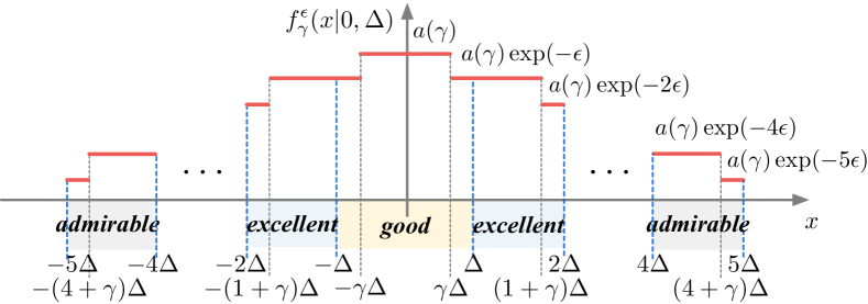
Figure 4: PDF of synonym substitution for the word “good”. The horizontal axis represents the embedding vector of each synonym. The vertical axis shows their probability.

4.1.2 Certification for Synonym Substitution

The embedding transformation $\phi_{S}$ is defined by substituting each word $x_{i}$’s embedding $w_{i}$ with its $a_{i}$th synonym’s $w_{i}^{a_{i}}$. $a_{i}$ decides the substitution of $x_{i}$, e.g., a closer synonym $w_{i}^{a_{i}}$ to $x_{i}$ has a smaller $a_{i}$. We assume $a_{i}$ follows a Staircase PDF, in which the probability of each synonym being selected is defined as Table III. Then, we provide the below robustness certification for the synonym substitution perturbation $\delta_{S}$.

Theorem 1.

Let $\phi_{S}:\mathcal{W}\times\mathbb{R}^{n}\to\mathcal{W}$ be the embedding substituting transformation based on a Staircase distribution $\varepsilon\sim\mathcal{S}_{\gamma}^{\epsilon}(w,\Delta)$ with PDF $f_{\gamma}^{\epsilon}(\cdot)$, and let $g_{S}$ be the smoothed classifier from any deterministic or random function $h$, as in (3). Suppose $y_{A},y_{B}\in\mathcal{Y}$ and $\underline{p_{A}},\overline{p_{B}}\in[0,1]$ satisfy:

$$\mathbb{P}(h(u\cdot\phi_{S}(w,\varepsilon))=y_{A})\geq\underline{p_{A}} \geq\overline{p_{B}}\geq$$

$$\max_{y_{B}\neq y_{A}} \mathbb{P}(h(u\cdot\phi_{S}(w,\varepsilon))=y_{B})$$

then $g_{S}(u\cdot\phi_{S}(w,\delta_{S}\cdot\Delta))=y_{A}$ for all $\|\delta_{S}\|_{1}\leq\mathtt{RAD}_{S}$, where

$$\small\mathtt{RAD}_{S}=\max\Big{\{}\frac{1}{2\epsilon}\log({\underline{p_{A}}}/{\overline{p_{B}}}),-\frac{1}{\epsilon}\log(1-\underline{p_{A}}+\overline{p_{B}})\Big{\}}.$$ (7)

Proof.

Proven in Appendix A.1. ∎

Theorem 1 states that any synonym substitution would not succeed as long as the $\ell_{1}$ norm of $\delta_{S}$ is smaller than $\mathtt{RAD}_{S}$. We can observe that the certified radius $\mathtt{RAD}_{S}$ is large under the following conditions: 1) the noise level $\epsilon$ is low, indicating a larger synonym size; 2) the probability of the top class $y_{A}$ is high, and those of other classes are low.

4.2 Certified Robustness to Word Reordering

4.2.1 Uniform-based Permutation

We assume that each position of the word is equally important to the prediction, and add a uniform distribution to the permutation matrix ($u$) to model permutation. Specifically, we simulate the uniform distribution by grouping the row vectors of $u$, then randomly reordering vector positions within the groups. For example, given a permutation matrix with $n$ row vectors $\{u_{i}\}$, we divide all $u_{i}$ uniformly and randomly into $n/\lambda$ groups with length $\lambda$ each. The row vector $u_{i}$ can be reordered randomly within the group. In this way, the noise added to each position is $1/\lambda$ (uniform). Also, $\lambda=n$ means randomly shuffling all row vectors of the entire permutation matrix. The proposed uniform smoothing method provides certification for the permutation perturbation $\delta_{R}$.

Theorem 2.

Let $\theta_{R}:\mathcal{U}\times\mathbb{Z}^{n}\to\mathcal{U}$ be a permutation based on a uniform distribution $\rho\sim\mathbf{U}[-\lambda,\lambda]$ and $g_{R}$ be the smoothed classifier from a base classifier $h$, as in (4). Suppose $g_{R}$ assigns a class $y_{A}$ to the input $u\!\cdot\!w$, and $\underline{p_{A}},\overline{p_{B}}\in(0,1)$. If

$$\mathbb{P}(h(\theta_{R}(u,\rho)\cdot w)=y_{A})\geq\underline{p_{A}} \geq\overline{p_{B}}\geq$$

$$\max_{y_{B}\neq y_{A}} \mathbb{P}(h(\theta_{R}(u,\rho)\cdot w)=y_{B}))$$

then $g_{R}(\theta_{R}(u,\delta_{R})\cdot w)=y_{A}$ for all permutation perturbations satisfies $\|\delta_{R}\|_{1}\leq\mathtt{RAD}_{R}$, where

$$\small\mathtt{RAD}_{R}=\lambda(\underline{p_{A}}-\overline{p_{B}})$$ (8)

Proof.

Proven in Appendix A.2. ∎

Theorem 2 states that any permutation would not succeed as long as $\delta_{R}<\mathtt{RAD}_{R}$ in Eq.(8). We can observe that the certified radius $\mathtt{RAD}_{R}$ is larger when $\lambda$ is higher, which requires more shuffling, or/and $\underline{p_{A}}$ is larger. The maximum certified radius is $\lambda$, which is the size of a reordering group. Note that both $\underline{p_{A}}$ and $\lambda$ depend on the noise magnitude.

4.3 Certified Robustness to Word Insertion

Word insertion employs a combination of permutation $\theta_{I}$ and embedding transformation $\phi_{I}$. Recall that the only transformation performed on the permutation matrix is to shuffle the position of $u_{i}$. Hence, we utilize the uniform-based permutation with the noise level set as the number of words ($n$), i.e., $\theta_{I}(u,\rho)=\theta_{R}(u,\rho)$, where $\rho\sim\mathbf{U}[-n,n]$. On the other hand, embedding insertion involves replacing $w_{n-m^{\prime}+i}$ with an unrestricted inserted embedding $w_{in}^{j}$, which sets it apart from synonym substitution. To address the challenge of unrestricted embedding insertion, we propose a Gaussian-based smoothing method for the certification.

4.3.1 Gaussian-based Embedding Insertion

We consider the embedding matrix as a whole, the length of which is $n\times d$, where $d$ is the dimension of each embedding vector. We add Gaussian noise to the embedding matrix directly, similar to adding independent identically distributed Gaussian noise to each pixel of an image. We invoke Theorem 1 in [22] as

Theorem 3.

Let $\phi_{I}:\mathcal{W}\times\mathbb{R}^{n\times d}\to\mathcal{W}$ be the embedding insertion transformation based on Gaussian noise $\varepsilon\sim\mathcal{N}(0,\sigma^{2}I)$ and $\theta_{I}$ be the perturbation as same as $\theta_{R}$ based on a uniform distribution $\rho\sim\mathbf{U}[-n,n]$. Let $g_{I}$ be the smoothed classifier from a base classifier $h$ as in (2), and suppose $y_{A},y_{B}\in\mathcal{Y}$ and $\underline{p_{A}},\overline{p_{B}}\in[0,1]$ satisfy:

$$\mathbb{P}(h(\theta_{I}(u,\rho)\cdot\phi_{I}(w,\varepsilon)))= \ y_{A})\geq\underline{p_{A}}\geq\overline{p_{B}}\geq$$

$$\max_{y_{B}\neq y_{A}} \mathbb{P}(h(\theta_{I}(u,\rho)\cdot\phi_{I}(w,\varepsilon))=y_{B}))$$

then $g_{I}(\theta_{I}(u,\delta_{R})\cdot\phi_{I}(w,\delta_{I}))=y_{A}$ for all $\|\delta_{R}\|_{1}<\mathtt{RAD}_{R}$ as in Eq.(8) and $\|\delta_{I}\|_{2}<\mathtt{RAD}_{I}$ where

$$\small\mathtt{RAD}_{I}=\frac{\sigma}{2}(\Phi^{-1}(\underline{p_{A}})-\Phi^{-1}(\overline{p_{B}}))$$ (9)

Theorem 3 states that $g_{I}$ can defend against word insertion transformation as long as the conditions about $\delta_{R}$ and $\delta_{I}$ are satisfied simultaneously. We observe that the certified radius $\mathtt{RAD}_{I}$ is large when the noise level $\sigma$ is high.

4.3.2 Combination of Two Perturbations

The certified radii of Eq.(8) and Eq.(9) ensure the robustness of the smoothed classifier against permutation $\theta_{I}$ or embedding insertion $\phi_{I}$, respectively. However, the word insertion is a combination of $\theta_{I}$ and $\phi_{I}$. Next, we propose Theorem 4 to provide certified robustness for the combination of them.

Theorem 4.

If a smoothed classifier $g$ is certified robust to permutation perturbation $\delta_{u}$ as defined in Eq.(10), and to embedding permutation $\delta_{w}$ as defined in Eq.(11), then $g$ can provide certified robustness to the combination of perturbations $\delta_{u}$ and $\delta_{w}$ as defined in Eq.(12) assuming $\theta(u,\rho)$ is uniformly distributed in the permutation space.

$$\forall\delta_{u},\delta_{w},g(\theta(u\!+\!\delta_{u},\rho)\cdot\!\phi(w,\varepsilon))\!=\!g(\theta(u,\rho)\!\cdot\!\phi(w,\varepsilon))$$ (10)

$$\qquad\,\,\,\&\,g(\theta(u,\rho)\!\cdot\!\phi(w\!+\!\delta_{w},\varepsilon))\!=\!g(\theta(u,\rho)\!\cdot\!\phi(w,\varepsilon))$$ (11)

$$\implies g(\theta(u\!+\!\delta_{u},\rho)\!\cdot\!\phi(w\!+\!\delta_{w},\varepsilon))\!=\!g(\theta(u,\rho)\!\cdot\!\phi(w,\varepsilon))$$ (12)

Proof.

Proven in Appendix A.3. ∎

Thus, when the certified radii $\mathtt{RAD}_{R}$ and $\mathtt{RAD}_{I}$ are derived w.r.t. $\delta_{u}$ and $\delta_{w}$ in two spaces using Eq.(8) and Eq.(9), respectively, then $\theta(u,\delta_{u})\cdot\phi(w,\delta_{w})$ is within the certified region of $g$ as long as both $\delta_{u}<\mathtt{RAD}_{R}$ and $\delta_{w}<\mathtt{RAD}_{I}$ hold.

4.4 Certified Robustness to Word Deletion

Similarly, a completely uniform shuffling of the orders is performed on permutation, denoted as $\theta_{D}(u,\rho)=\theta_{R}(u,\rho)$, where $\rho$ is drawn from $\mathbf{U}[-n,n]$. Recall that embedding deletion is modeled as a change in the embedding state from $b_{i}=1$ to $b_{i}=0$. To certify against the $\ell_{0}$-norm of embedding deletion perturbation (as the number of deleted words), we propose a Bernoulli-based smoothing method.

4.4.1 Bernoulli-based Embedding Deletion

The transition of the embedding state ($a_{i}$) can be considered to follow the Bernoulli distribution $\mathbf{B}(n,p)$, where $n$ is the total number of words in the text. Each word embedding can be transformed to $w_{\texttt{<pad>}}$ with probability $p$ and maintained with $1-p$, i.e, $\mathbb{P}(b_{i}=1\to b_{i}=0)=p$ and $\mathbb{P}(b_{i}=1\to b_{i}=1)=1-p$. The $w_{\texttt{<pad>}}$ cannot be transformed into a word embedding since we cannot recover the deleted words when they are removed from the text. It can be denoted as $\mathbb{P}(b_{i}=0\to b_{i}=1)=0$.

Theorem 5.

Let $\phi_{D}:\mathcal{W}\times\{0,1\}^{n}\to\mathcal{W}$ be the embedding deletion transformation based on Bernoulli distribution $\varepsilon\sim\mathbf{B}(n,p)$ and $\theta_{D}$ be the perturbation same as $\theta_{R}$ based on a uniform distribution $\rho\sim\mathbf{U}[-n,n]$. Let $g_{D}$ be the smoothed classifier from a base classifier $h$, as in (2) and suppose $y_{A},y_{B}\in\mathcal{Y}$ and $\underline{p_{A}},\overline{p_{B}}\in[0,1]$ satisfy:

$$\mathbb{P}(h(\theta_{D}(u,\rho)\cdot\phi_{D}(w,\varepsilon))) =y_{A})\geq\underline{p_{A}}\geq\overline{p_{B}}\geq$$

$$\max_{y_{B}\neq y_{A}} \mathbb{P}(h(\theta_{D}(u,\rho)\cdot\phi_{D}(w,\varepsilon))=y_{B}))$$

then $g_{D}(\theta_{D}(u,\delta_{R})\cdot\phi_{D}(w,\delta_{D}))=y_{A}$ for all $\|\delta_{R}\|_{1}<\mathtt{RAD}_{R}$ as in Eq.(8) and $\|\delta_{D}\|_{0}<\mathtt{RAD}_{D}$, where

$$\mathtt{RAD}_{D}=\operatorname*{arg\,max}\delta,$$ (13)

$$\textrm{\ s.t.\ }\tbinom{z_{\max}}{\delta}\leq\underline{p_{A}}/\overline{p_{B}},$$

$$\qquad z_{\max}\!=\!\operatorname*{arg\,max}z,\textrm{\ s.t.\ }\tbinom{n}{z}p^{z}(1-p)^{(n-z)}\!\leq\!\overline{p_{B}}.$$

Proof.

Proven in Appendix A.4. ∎

Theorem 5 states that $g_{D}$ can defend against any word deletion transformation as long as the conditions about $\delta_{R}$ and $\delta_{D}$ are met. We observe that the certified radius $\mathtt{RAD}_{D}$ is large when the total number of words $n$ is small.

4.5 Universality of Certification for Insertion

All four adversarial operations are essentially transformations of the embedding vector. Hence, our certification for the word insertion, a combination of uniform-based permutation ($\theta_{I}$) and Gaussian-based embedding transformation ($\phi_{I}$), is applicable to all the four operations. The synonym substitution operation only employs the embedding transformation ($\theta_{I}$), with the embedding perturbation being the sum of the embedding distances of the replaced synonyms. Word reordering is a simple version of word insertion, using only permutation ($\theta_{I}$). Word deletion, on the other hand, uses both permutation ($\theta_{I}$) and embedding transformation ($\theta_{I}$), with its embedding perturbation being the sum of the embedding distances of the deleted words.

5 Practical Algorithms

5.1 Training

Given the word operation $T\in\{S,R,I,D\}$, we aim to generate a certified model against the corresponding word-level attack. As described in Algorithm 1, we first generate a set of embedding matrices $w$ with the pre-trained embedding layer $L_{emb}$. The permutation matrix $u$ is an identity matrix with the same length as $w$ (line 1). Then, we perform permutation and embedding transformations on $u$ and $w$ to generate the dataset $\mathcal{D}_{T}$. Finally, we update the model with the training dataset $\mathcal{D}_{T}$ and obtain the model $h$.

Algorithm 1 Training algorithm

1:Training dataset $\mathcal{D}=\{(x,y)_{i}\}$, operation $T$, pre-trained embedding layer $L_{emb}$, permutation $\theta_{T}$ with noise $\rho$, embedding transformation $\phi_{T}$ with noise $\varepsilon$

2:$u\cdot w\leftarrow L_{emb}(x)$ $\triangleright$ $u$ is $w$’s permutation matrix

3:$\mathcal{D}_{T}=\{(\theta_{T}(u,\rho)\cdot\phi_{T}(w,\varepsilon),y)_{i}\}$

4:$h\leftarrow$ Train the classification model with $\mathcal{D}_{T}$

5:return Classification model $h$

5.1.1 Enhanced Training Toolkit for Word Insertions

High-level Gaussian noise leads to distortion in the embedding space and results in barely model convergence. To address this issue, we develop a toolkit with three methods for the three steps in the training (see Figure 5). The toolkit is mainly used to improve the certified accuracy against word insertions, and it is also applicable to other operations.

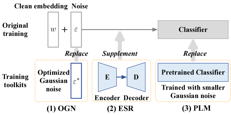
Figure 5: The training toolkit can enhance model accuracy by replacing or supplementing part of the training process.

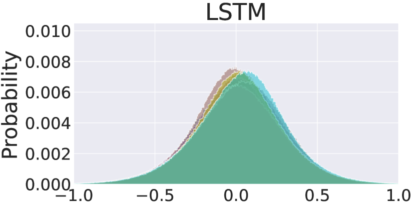
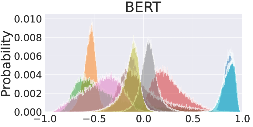
Figure 12: For LSTM and BERT, the distributions of the embedding elements for all words in ten randomly chosen dimensions. These distributions approximate Gaussian distributions with different means.

① Optimized Gaussian Noise (OGN). Inspired by the Anisotropic-RS [56], an appropriate mean value of Gaussian noise can improve the certified accuracy. We analyze the embedding vectors of all words and observe that each element in the embedding vectors approximates a Gaussian distribution with a nonzero mean, as illustrated in Figure 12. Consequently, we can enhance the certified accuracy by modifying the Gaussian noise of each dimension $\mathcal{N}(0,\sigma I^{2})\to\mathcal{N}(\mu_{i},\sigma I^{2})$, where $\mu_{i},\ i\in[1,d]$ denotes the average of the original embedding space of each dimension.

② Embedding Space Reconstruction (ESR). To mitigate the disturbance of the embedding space, we introduce an encoder-decoder architecture to reconstruct the clean embedding space. The encoder-decoder can also be viewed as sanitizing the additive noise. This method can effectively improve accuracy in small-dimension embedding space, such as with the $300$-dimension GloVe embedding and LSTM classifier, resulting in a $10\%$ increase in average accuracy.

③ Pre-trained Large Model (PLM). Fine-tuning from a pre-trained model is a typical training approach for large models. When applying high-level Gaussian noise to a large model, we can fine-tune it on a pre-trained large model trained with small Gaussian noise (e.g., $\sigma=0.1$). For instance, when adding Gaussian noise of $\sigma=1.5$ to the IMDB dataset and using BERT as the classifier, this approach can substantially enhance model accuracy from $50\%$ to $84\%$.

5.2 Certified Inference

The certified inference algorithm is identical to the classical randomized smoothing in [22]. We first obtain the embedding $u\cdot w$ of the test sample $x$ by the pre-trained embedding layer $L_{emb}$. Then, we utilize $\theta_{T}(u,\rho)\cdot\phi_{T}(w,\varepsilon)$ to draw $N$ samples by the $T$ transformation. Finally, we certify robustness on $N$ samples and output the robust prediction. Details are presented in Algorithm 2 in Appendix B.

6 Experiments

6.1 Experimental Setup

Datasets. We evaluate Text-CRS on three textual datasets, AG’s News (AG) [57], Amazon [58], and IMDB [59]. The AG dataset collects news articles (sentence-level), covering four topic classes. The Amazon dataset consists of positive and negative product reviews (document level). The IMDB dataset contains document-level movie reviews with positive and negative sentiments. The average sample lengths of them are $43$, $81$, and $215$, respectively.

Models and Embedding Layers. We conduct experiments on two common NLP models, LSTM [60] and BERT [41] with the pre-trained embedding layers. For LSTM, we use a 1-layer bidirectional LSTM with $150$ hidden units and the $300$-dimensional Glove word embeddings trained on $42$ billion tokens of web data from Common Crawl [40]. For BERT, we use a pre-trained $12$-layer bert-base-uncased model with $12$ attention heads. The pre-trained embedding layer in BERT outputs $768$-dimensional hidden features for each token. We freeze the pre-trained embedding layer in both LSTM and BERT and only update the parameters of the classification models.

Evaluation Metric. We report the model accuracy on the clean test set for vanilla training (Clean vanilla) and certified robust training (Clean Acc.) (see Table IX). Under robust training, we also evaluate the certified accuracy, defined as the fraction of the test set classified correctly and certified robust. We uniformly select $500$ examples from the clean test set of each dataset. For each example, we use $N_{0}=100$ samples for selecting the most likely class $y_{A}$ and $N=10^{5}$ samples for estimating confidence lower bound $\underline{p_{A}}$. We set $\alpha=0.001$ for certification with at least 99.9% confidence. To test the model’s robustness against unseen attacks, we evaluated Text-CRS against five real-world attacks (TextFooler[9], WordReorder[49], SynonymInsert[50], BAE-Insert[10], and InputReduction[13] w.r.t. four word-level adversarial operations), and generate $1,000$ successful adversarial examples for each dataset and model. We calculate the attack accuracy of the vanilla model under attack as the percent of unsuccessful adversarial examples divided by the number of attempted examples (see Table X). For Text-CRS against these attacks, we uniformly select 500 successful adversarial examples for each attack and evaluate the certified accuracy with $N=2\times 10^{4}$. Since the baselines can only certify against substitution operations, we evaluate their certified accuracy against TextFooler. For the other attacks, we evaluate their empirical accuracy, the percent of adversarial examples correctly classified (no certification).

Noise Parameters. We use three levels of noise (i.e., Low, Medium (Med.), and High) for the four smoothing methods (see Table IV). Synonym substitution based on the Staircase PDF uses the size of the lexicon ($s$) to control the PDF’s sensitivity, i.e., $\epsilon=5/s$. For other parameters in the staircase PDF, we fix the interval size of a word as $\Delta=1$ and set an equal probability within each interval, i.e., $\gamma=1$. Uniform-based permutation specifies the noise with the length of the reordering group, i.e., the noise PDF of $\mathcal{U}[-\lambda,\lambda]$ is $1/2\lambda$. While using uniform permutation in word insertion and deletion, we set the noise level to $n$, i.e., reordering the entire text. Gaussian-based embedding insertion uses the standard deviation $\sigma$ to specify the noise. We set different $\sigma$ in LSTM and BERT models due to different embedding dimensions and magnitudes. Bernoulli-based smoothing uses the deletion probability $p$ of each word as the noise.

Table IV: Noise parameters for adversarial operations

Operations	Substitution	Reordering	Insertion		Deletion
Noise	$s$	$2\lambda$	$2\lambda$	$\sigma$(LSTM, BERT)	$2\lambda$	$p$
Low	$50$	$n/4$	$n$	$0.1$, $0.5$	$n$	$0.3$
Med.	$100$	$n/2$	$n$	$0.2$, $1.0$	$n$	$0.5$
High	$250$	$n$	$n$	$0.3$, $1.5$	$n$	$0.7$

Training Toolkit. ① In OGN, we use the average of the parameters of the pre-trained embedding layers (i.e., Glove word embeddings for LSTM and BERT’s pre-trained embedding layer for BERT) as the mean value of Gaussian noise in each dimension ($\mu_{i}$). ② In ESR, we utilize two fully-connected layers as the encoder-decoder for LSTM. ③ In PLM, we set the learning rate to $0.00003$, training epochs to $10$, and the Gaussian noise level to $\sigma=0.1$ for training the pre-trained BERT model with Gaussian noise.

Baselines. We compare our methods with two SOTA randomized smoothing-based certified defenses, SAFER [29] and CISS [31]. 1) SAFER certifies against synonym substitution. Following the same setting [29, 25] for the synonym substitution, we construct synonym sets by the cosine similarity of Glove word embeddings [40] and sort all synonyms in the descending order of similarity. 2) CISS is an IBP and randomized smoothing-based method against word substitution. CISS provides only the training and certification pipelines for the BERT model. Thus, we only compare our Text-CRS with CISS under the BERT model.

Note that the smoothed models against substitution, reordering, and deletion operations are trained without the use of training toolkits. The training toolkits can further improve their certification performance.

6.2 Experimental Results

6.2.1 Evaluating Adversarial Examples using ChatGPT

We assess the practical significance of textual adversarial examples by evaluating whether ChatGPT (version “gpt-3.5-turbo-0301”) can determine if a successful adversarial example is semantically similar to the original text. Specifically, we request ChatGPT to assess the semantic similarity (categorized as “Yes” or “No”) and calculate the cosine similarity between the adversarial and original texts. Table V shows the deception rate, which represents the percent of successful adversarial examples that ChatGPT considered semantically similar to the original texts, as well as the cosine similarity of total successful examples, and the cosine similarity of the examples that deceive ChatGPT. The results show an average of $73\%$ of all successful adversarial examples can deceive ChatGPT, highlighting the severe threat posed by textual adversarial examples. Furthermore, we observe that longer texts, such as those in Amazon and IMDB, are easier to fool ChatGPT, due to the challenges in detecting small perturbations in longer texts. Finally, the cosine similarities of all our successful adversarial examples are high, particularly in the case of SynonymInsert and BAE-Insert attacks, unveiling that word insertion can effectively fool the vanilla model with minimal perturbations.

Table V: Evaluation on adversarial examples by ChatGPT.

Metric	Deception rate			Cosine similarity (success / deception)
Attack type	AG	Amazon	IMDB	AG	Amazon	IMDB
TextFooler	58%	78%	85%	0.92 / 0.97	0.81 / 0.94	0.97 / 0.99
WordReorder	63%	53%	60%	0.84 / 0.95	0.79 / 0.91	0.90 / 0.97
SynonymInsert	75%	89%	85%	0.97 / 0.98	0.95 / 0.98	0.98 / 0.99
BAE-Insert	66%	88%	71%	0.96 / 0.97	0.91 / 0.97	0.97 / 0.99
InputReduction	75%	78%	73%	0.89 / 0.96	0.85 / 0.93	0.94 / 0.98
Average	67%	77%	75%	0.92 / 0.97	0.86 / 0.95	0.95 / 0.98

6.2.2 Certified Robustness of Text-CRS

Table VI: Certified accuracy under adversarial operations. We compare the substitution with SAFER[29] and CISS[31], and provide a benchmark for other operations.

Dataset (Model)	Clean vanilla	Noise	Synonym substitution			Reordering	Insertion	Deletion
			SAFER	CISS	Ours	Ours	Ours	Ours
AG (LSTM)		Low	86.4%		88.8%	92.4%	88.6%	91.2%
	91.79%	Med.	85.2%	-	88.6%	91.6%	88.2%	90.2%
		High	83.2%		87.0%	92.4%	82.8%	88.4%
AG (BERT)		Low	92.0%	85.6%	92.8%	95.6%	93.6%	94.6%
	93.68%	Med.	89.2%	86.8%	92.0%	93.6%	93.0%	93.3%
		High	87.2%	85.6%	91.2%	94.4%	91.2%	92.8%
Amazon (LSTM)		Low	82.8%		82.6%	87.2%	85.2%	88.8%
	89.82%	Med.	80.0%	-	82.4%	85.8%	79.0%	88.8%
		High	80.2%		83.6%	88.4%	75.6%	87.2%
Amazon (BERT)		Low	90.2%	84.4%	93.6%	94.8%	94.4%	93.8%
	94.35%	Med.	86.4%	83.4%	90.2%	93.6%	92.6%	91.8%
		High	86.2%	83.2%	87.6%	93.8%	89.0%	88.6%
IMDB (LSTM)		Low	77.8%		84.0%	88.8%	82.2%	86.0%
	86.17%	Med.	77.6%	-	81.6%	84.6%	79.2%	85.4%
		High	77.0%		78.8%	83.4%	71.4%	84.8%
IMDB (BERT)		Low	86.4%	84.8%	89.6%	92.2%	90.8%	91.4%
	91.52%	Med.	82.8%	82.4%	83.6%	92.4%	88.4%	90.2%
		High	75.8%	84.0%	78.8%	91.8%	84.0%	89.2%

Table VI summarizes the certified accuracy of Text-CRS against four word-level operations on different datasets, models, and noise. For synonym substitution, we use the same synonym set and noise parameters as SAFER. The results demonstrate that Text-CRS outperforms SAFER for all noise levels under three datasets and two models. Specifically, Text-CRS is more accurate than SAFER (under LSTM and BERT) and CISS (under BERT) in all the settings. To our best knowledge, Text-CRS is the first to provide certified robustness for word reordering, insertion, and deletion. Compared to Clean vanilla, Text-CRS sacrifices only a small fraction of accuracy. Across all $24$ settings, including $4\ \textrm{operations}\times\!\ 3\ \textrm{datasets}\times\!\ 2\ \textrm{models}$, Text-CRS provides an average best certified accuracy of $90.2\%$ (bold), with a small drop compared to the average vanilla accuracy of $91.22\%$.

Moreover, our methods for substitution, insertion, and deletion achieve the best certified accuracy with low noise, indicating that smaller noise has less impact on model performance. Conversely, the best certified accuracy for reordering can be achieved at low, medium, or high noise levels, as the results suggest that robust training with reordering operations has little effect on the model accuracy. Regarding model structures, Text-CRS outperforms SOTA methods under LSTM and achieves superior performance under BERT, with a certified accuracy that is closer to or exceeds that of Clean vanilla. Regarding the dataset, Text-CRS demonstrates better performance on large-scale datasets, such as IMDB, where the substitution method outperforms SAFER by $1.6\%$ and $4.7\%$ on AG and IMDB, and CISS by $6.0\%$ and $4.8\%$ on AG and IMDB, respectively.

6.2.3 Certified Accuracy under Different Radii

We examine the effect of certified radii with different noise levels on the certified accuracy against four adversarial operations, as depicted in Figure 6 to 9. The results indicate that the certified accuracy declines as the radius increases, and it abruptly drops to zero at a certain radius threshold, consistent with the results in the image domain [22]. Moreover, the impact of noise level on certified accuracy increases with the magnitude of the noise, while a large noise level can improve the certified radius. In other words, selecting a larger noise is necessary while aiming for a wider certification range. Thus, it is crucial to choose an appropriate smoothing magnitude for each specific setting carefully.

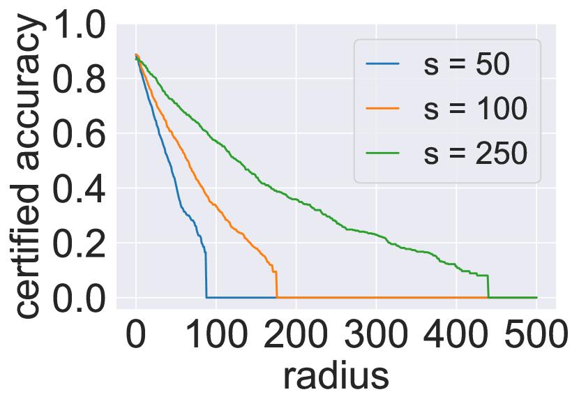
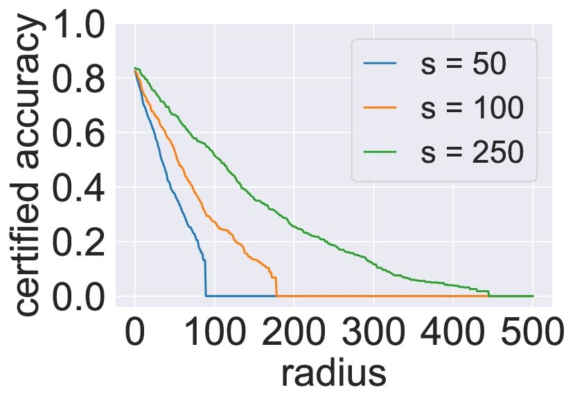
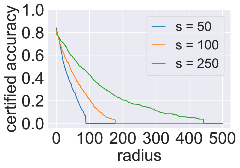
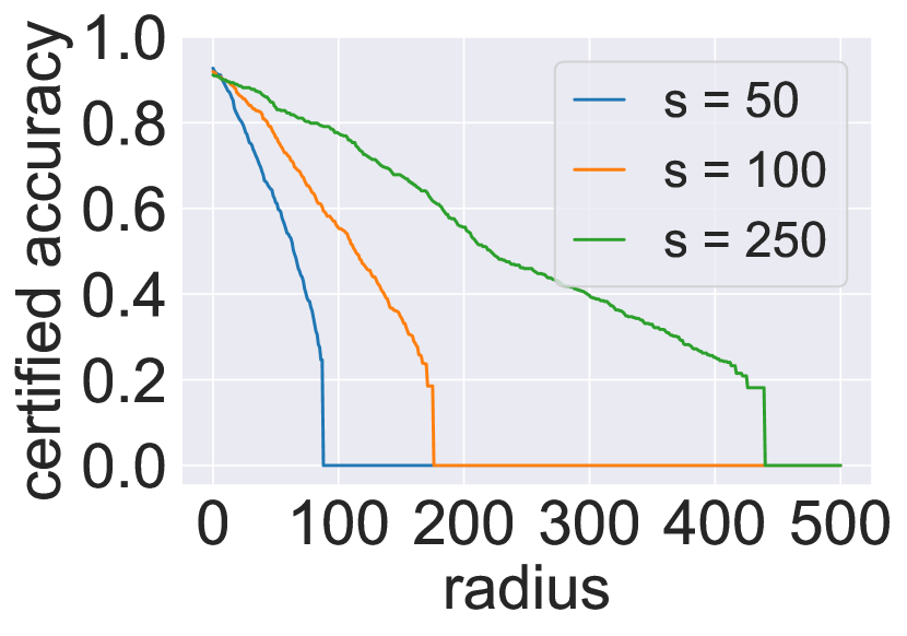
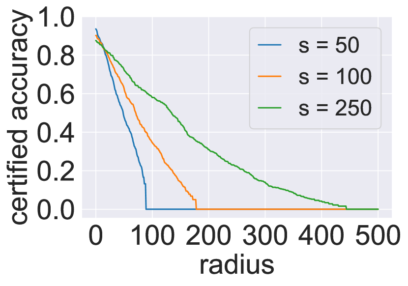
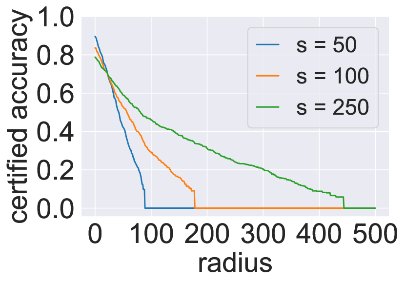
Figure 6: Certified accuracy at different radii against synonym substitution. Datasets from left to right: AG, Amazon, and IMDB; Models: top-LSTM and bottom-BERT.

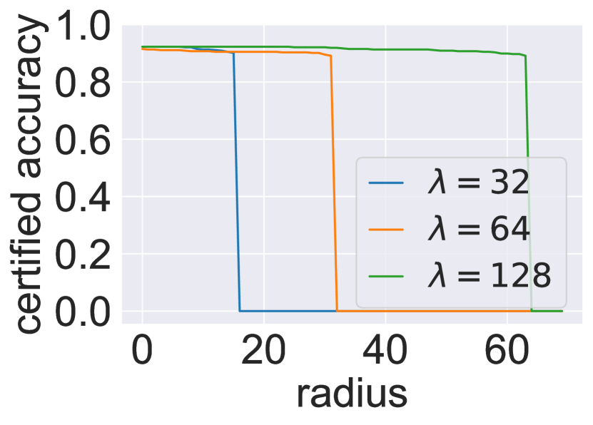
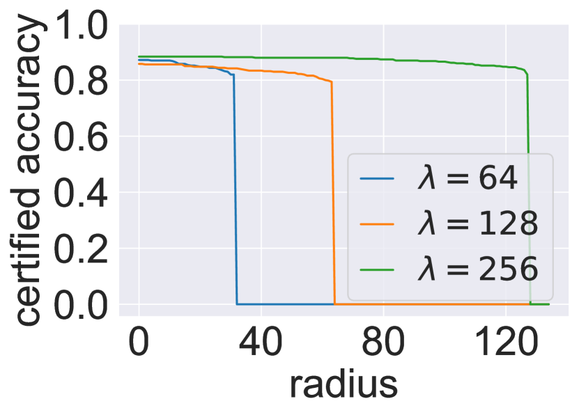
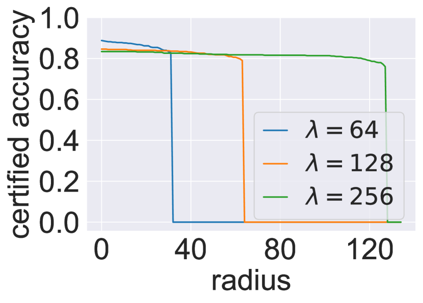
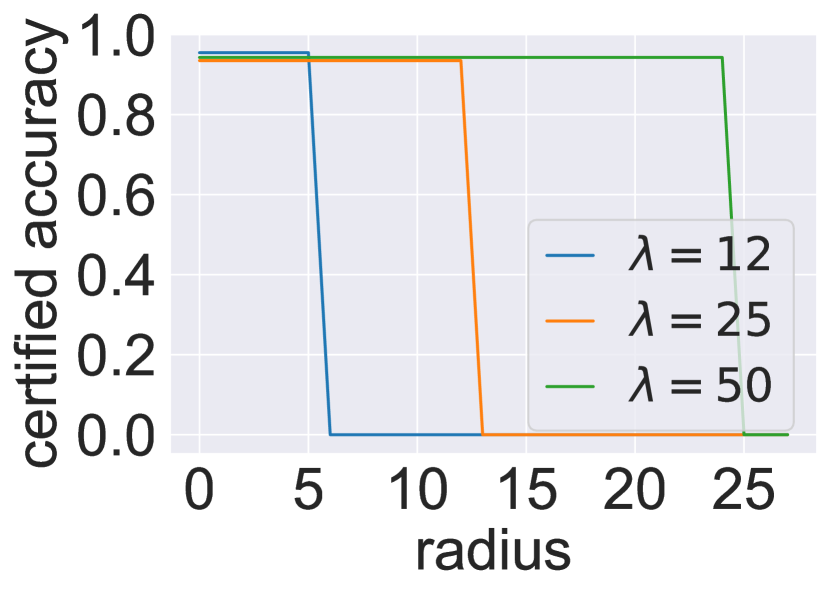
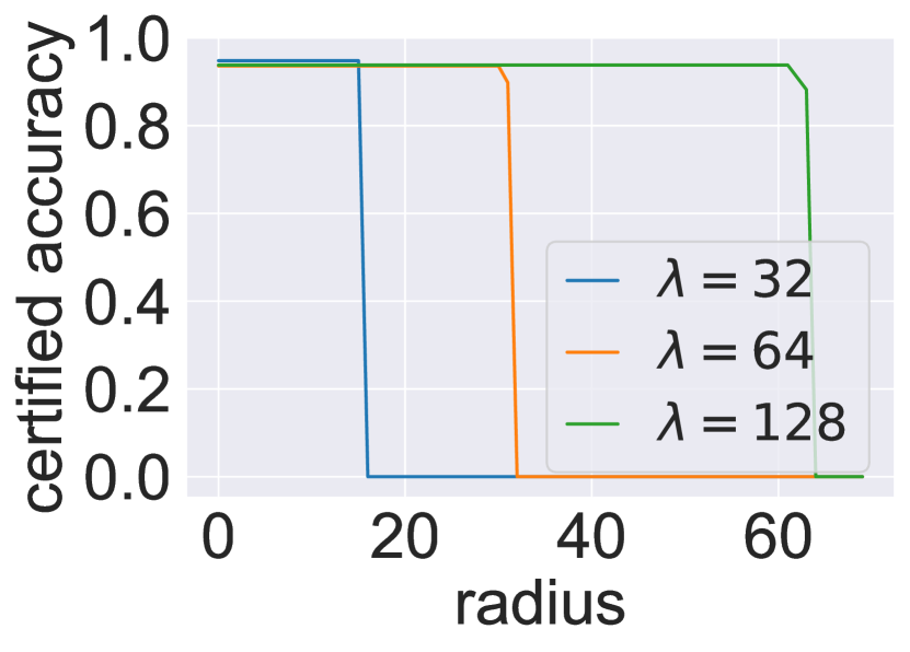
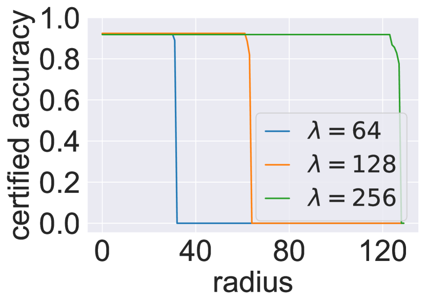
Figure 7: Certified accuracy at different radii against word reordering. Datasets from left to right: AG, Amazon, and IMDB; Models: top-LSTM and bottom-BERT.

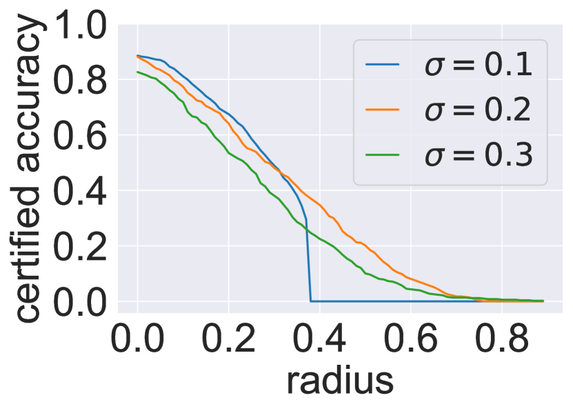
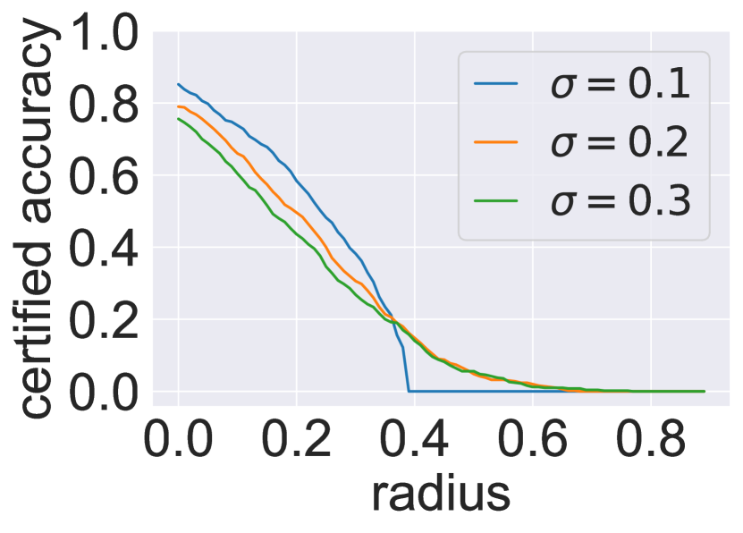
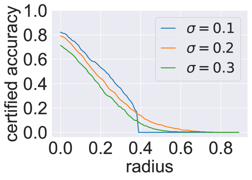
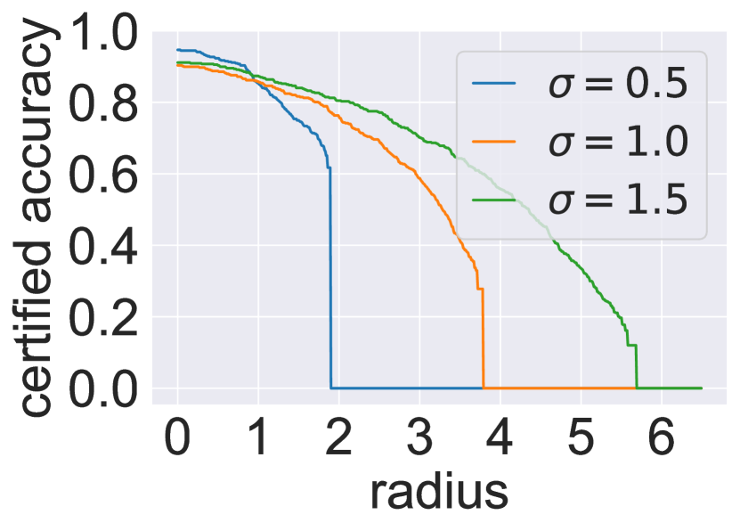
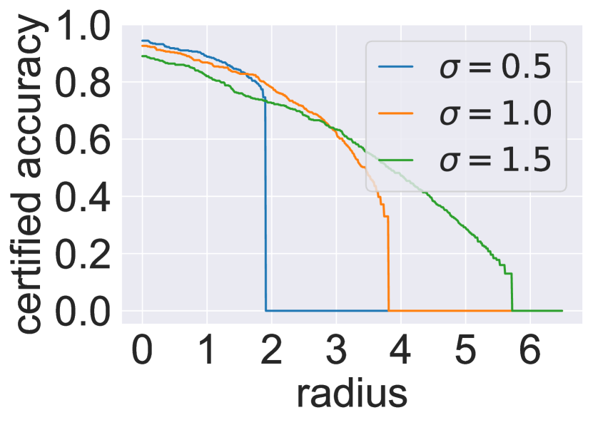
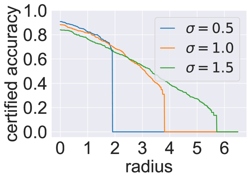
Figure 8: Certified accuracy at different radii against word insertion. Datasets from left to right: AG, Amazon, and IMDB; Models: top-LSTM and bottom-BERT.

Table VII: Comparison of certified accuracy of Text-CRS, SAFER [29] and CISS [31] under different attacks. “$*$” indicates that SAFER and CISS cannot certify operations other than substitution, resulting in a certified accuracy of $0\%$ for these attacks, so we report their empirical accuracy. “-” indicates that BAE-Insert and CISS cannot be performed on LSTM.

		TextFooler[9]			WordReorder[49]			SynonymInsert[50]			BAE-Insert[10]			InputReduction[13]
Dataset (Model)	Vanilla	SAFER	CISS	Ours	SAFER∗	CISS∗	Ours	SAFER∗	CISS∗	Ours	SAFER∗	CISS∗	Ours	SAFER∗	CISS∗	Ours
AG (LSTM)	0%	90.4%	-	91.2%	75.4%	-	89.2%	77.6%	-	84.2%	-	-	-	65.8%	-	78.4%
AG (BERT)	0%	93.2%	71.4%	93.6%	86.8%	83.8%	87.6%	77.8%	74.6%	83.6%	79.8%	74.0%	79.4%	55.8%	59.0%	68.4%
Amazon (LSTM)	0%	82.4%	-	83.4%	78.0%	-	91.2%	64.0%	-	71.8%	-	-	-	71.2%	-	74.2%
Amazon (BERT)	0%	87.0%	75.4%	90.8%	82.0%	88.0%	84.6%	67.8%	67.8%	80.6%	70.4%	70.4%	71.2%	68.6%	74.0%	82.0%
IMDB (LSTM)	0%	82.0%	-	84.6%	77.8%	-	86.0%	66.8%	-	69.6%	-	-	-	68.8%	-	77.0%
IMDB (BERT)	0%	83.8%	25.6%	84.4%	80.2%	24.8%	83.0%	76.8%	31.6%	86.2%	77.0%	33.0%	80.6%	70.6%	29.8%	82.8%
Average	0%	86.5%	57.5%	88.0%	80.0%	65.5%	86.9%	71.8%	58.0%	79.3%	75.7%	59.1%	77.1%	66.8%	54.3%	77.1%

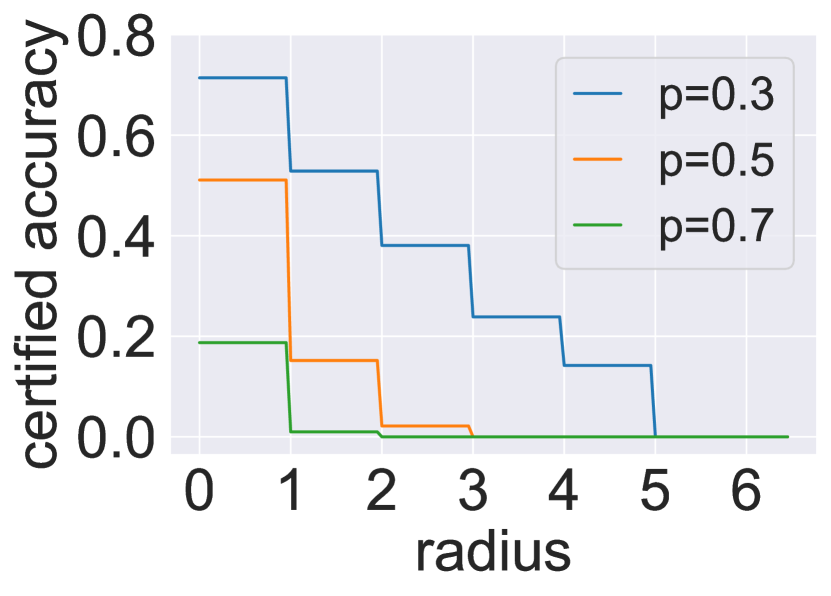
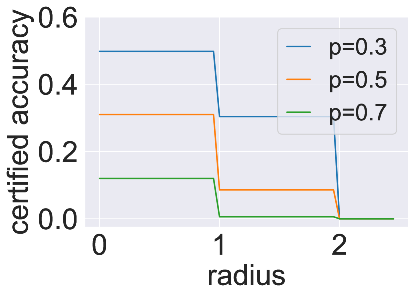
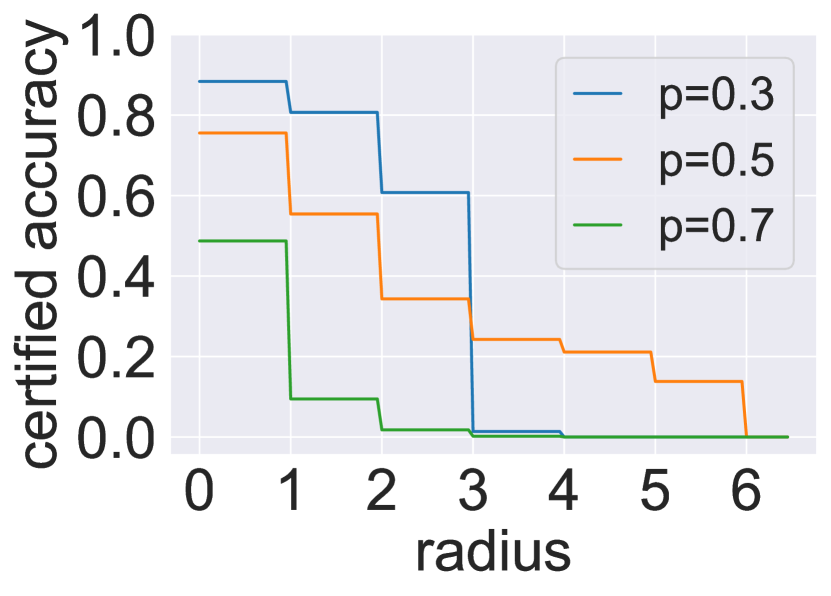
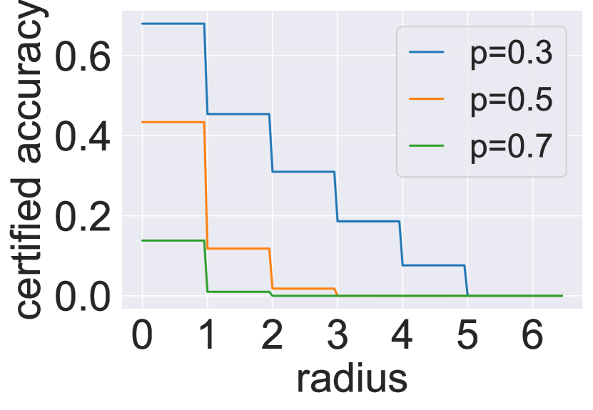
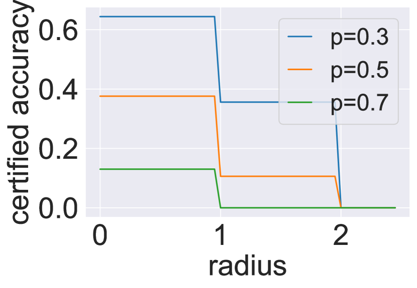
Figure 9: Certified accuracy at different radii against word deletion. Datasets from left to right: AG, Amazon, and IMDB; Models: top-LSTM and bottom-BERT.

Figure 6 depicts the certified accuracy with different sizes of synonym sets. A radius of $\mathtt{RAD}_{S}\!=\!200$ for a sentence with a length of 50 implies that each word can be substituted with its four closest synonyms in the thesaurus. In such cases, the prediction results of the smoothed classifier remain the same as the original sentence. Figure 7 depicts the certified accuracy under different sizes of shuffling groups. The radius $\mathtt{RAD}_{R}\!=\!100$ indicates that Text-CRS certifies a text in which the sum of all word positions changes is less than $100$. Figure 8 presents the certified accuracy under different Gaussian noise. The radius $\mathtt{RAD}_{I}$ denotes the cumulative embedding $\ell_{2}$ distances between the original and the inserted word. To illustrate the practical significance of our radius, we calculate the $\ell_{2}$ distance between $65,713$ words and their closest top-$k$ embeddings under Glove embedding space and BERT embedding space (see Figure 10). The results indicate that under $\mathtt{RAD}_{I}\!=\!0.2$, the LSTM model (using GloVe embedding space) could withstand $\sim$7% of random word insertions among all the top-3 closest words. The BERT model performs better than LSTM, which can withstand $\sim$53% and $\sim$11% of random word insertions among the top-5 and top-50 closest embeddings, respectively, under $\mathtt{RAD}_{I}\!=\!2$. Figure 9 shows the certified accuracy under different word deletion probabilities, where a radius $\mathtt{RAD}_{D}\!=\!2$ indicates that up to two words can be deleted while ensuring the certified robustness of the text. Note that Figure 7 also shows the certified radius on word position changes in word insertion and deletion operations.

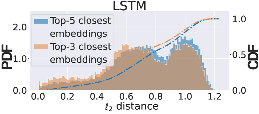
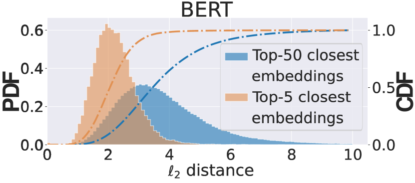
Figure 10: PDF and CDF of top-$k$ closest embeddings in Glove (LSTM) and BERT embedding space.

Furthermore, regarding the word reordering, the noise level has little effect on the certified accuracy, particularly for the BERT, which uses a transformer structure to represent each word as a weighted sum of all input word embeddings [44]. Consequently, the prediction of BERT contains information about every word, and the reordering of words has a reduced effect on the resultant output of BERT. This implies that we can choose a large noise level to achieve high certified accuracy while obtaining the largest certified radius simultaneously. It is consistent with our reordering strategies in word insertion and deletion operations.

Table VIII: Certified accuracy of word insertion smoothing method against different attacks.

Dataset (Model)	Text- Fooler[9]	Word- Reorder [49]	Synonym- Insert[50]	BAE- Insert [10]	Input- Reduction[13]
AG (LSTM)	81.6%	85.0%	84.2%	-	70.0%
AG (BERT)	83.4%	90.2%	83.6%	79.4%	58.4%
Amazon (LSTM)	75.4%	83.6%	71.8%	-	70.4%
Amazon (BERT)	82.8%	84.4%	80.6%	71.2%	74.4%
IMDB (LSTM)	64.2%	87.2%	69.6%	-	68.8%
IMDB (BERT)	81.4%	87.0%	86.2%	80.6%	77.4%
Average	78.1%	86.2%	79.3%	77.1%	69.9%

6.2.4 Certified Accuracy against Unseen Attacks

We select the noise parameters w.r.t. the highest certified accuracy for the three methods and evaluate the robustness under these noises. Table VII displays the certified accuracy of three methods against five types of attacks. The ‘Vanilla’ column shows that the accuracy is $0\%$ for all successful adversarial examples on the vanilla models. Text-CRS demonstrates an average certified accuracy that is 64% and 70% higher than SAFER and CISS, respectively, across all attacks. Specifically, our method achieves the highest certified accuracy for the TextFooler attack, surpassing SAFER and CISS in all settings. SAFER and CISS only provide certification against substitution attacks, resulting in $0\%$ certified accuracy for WordReorder to InputReduction attacks. Therefore, we evaluate their empirical accuracy against these attacks. It is important to note that empirical accuracy is generally higher than certified accuracy under the same setting. On average, our certified accuracy is still $5.5\%$ and $22.8\%$ higher than the empirical accuracy of SAFER and CISS, respectively.

6.2.5 Word Insertion Smoothing vs. All Attacks (Universality)

We evaluate the certified accuracy of the word insertion smoothing against all aforementioned attacks (universality), as shown in Table VIII. On average, our word insertion smoothing achieves a certified accuracy of $78.1\%$. It can certify against all attacks, though with a slight performance drop compare to the operation-specific methods in our Text-CRS. However, its certified accuracy is still higher than the empirical accuracy of SAFER and CISS, except the SAFER against TextFooler (substitution operation-specific). Therefore, the word insertion smoothing in Text-CRS is suitable for providing high certified accuracy when the attack type is unknown (due to its high universality), while higher certified accuracy can be achieved using specific methods in Text-CRS to defend known attacks.

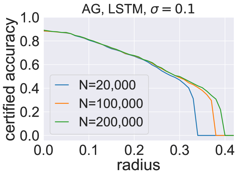
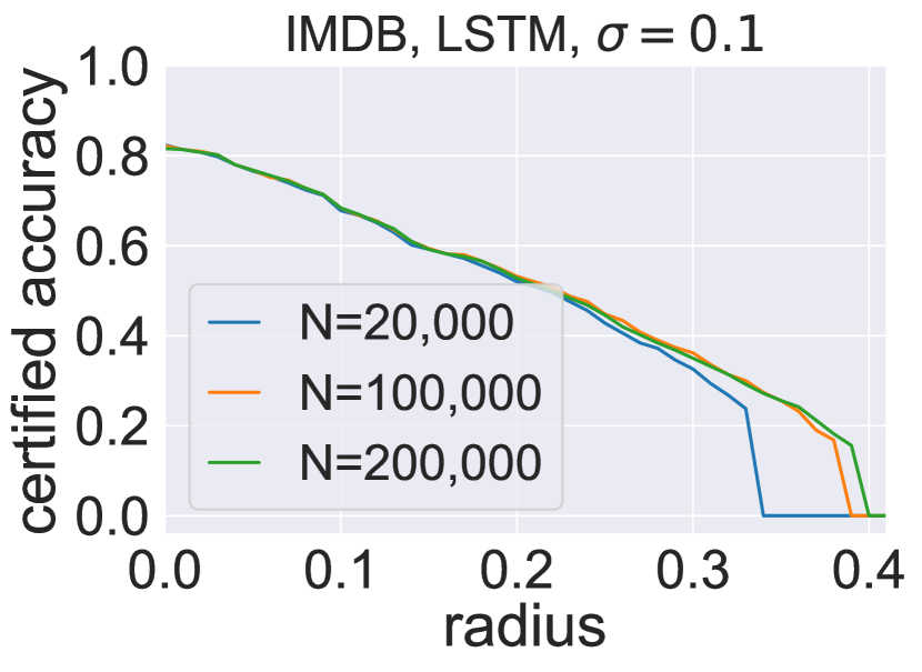
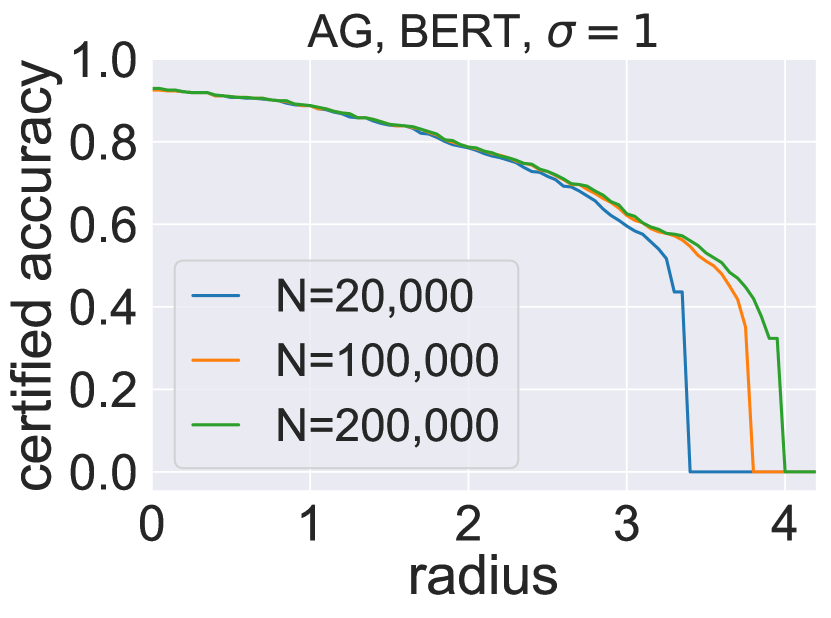
Figure 11: Impact of the number of samples ($N$) on certified accuracy against word insertion under LSTM and BERT.

6.2.6 Impact of the Number of Samples ($N$)

Figure 11 show that as the number of samples for estimation ($N$) increases, the certified accuracy also increases and the certified radius becomes larger, since the estimation for $\underline{p_{A}}$ and $\overline{p_{B}}$ becomes tighter. The impact of $N$ on the certified accuracy of the IMDB dataset is greater than that of the AG dataset, since longer inputs have a larger noise space, necessitating more samples to approximate $\underline{p_{A}}$ and $\overline{p_{B}}$.

7 Related Work

Word-level Adversarial Attacks. These attacks aim to mislead the model by modifying the words in four adversarial operations: synonym substitution [62, 7, 9, 63, 64, 17], word reordering [49, 65, 66, 67], word insertion [50, 12, 10, 68], and word deletion [13, 49, 69]. For instance, Ren et al. [7] propose a greedy PWWS algorithm to determine the replacement order of words in a sentence and the selection of synonyms. Tan et al. [64] proposed Morpheus, which generates plausible and semantically similar adversarial texts by replacing the words with their inflected form. Moradi and Samwald [49] investigated the sensitivity of NLP systems to such operation. Morris et al. [50] proposed TextAttack, including a basic strategy of inserting synonyms of words already in the text. Li et al. [12] proposed CLARE, which, similar to BAE, also employs masked language models to predict newly inserted <mask> tokens in the text and replace them. These adversarial texts have improved syntactic and semantic consistency compared to directly inserting synonym words [10]. Feng et al. [13] proposed input reduction, which involves the iterative removal of the least significant words from the clean text.

Certified Defenses against Word-level Adversarial Operations. These methods rely on interval bound propagation (IBP) [25, 70, 26], zonotope abstraction [27, 28] or randomized smoothing [29, 30]. IBP [25] and zonotope abstraction [27] are both linear relaxation methods, which calculate the lower and upper bound of the model output and then minimize the worst-case loss for certification. Ko et al. [26] introduced POPQORN, which uses linear functions to bound the nonlinear activation function in RNN. On more complicated Transformer models, Bonaert et al. [28] proposed DeepT to certify against synonym substitution operations based on multi-norm zonotope abstract interpretation. However, IBP and zonotope abstraction methods are not scalable, and few can tightly certify large-scale pre-trained models, such as BERT. To address this challenge, Ye et al. [29] proposed SAFER, which leverages randomized smoothing to provide $\ell_{0}$ certified robustness against synonym substitutions. Zhao et al. [31] proposed CISS, which combines the IBP encoder and randomized smoothing to guarantee $\ell_{2}$ robustness against word substitution attacks. However, since CCIS maps the input into a semantic space, only the certified radius in the semantic space is available, not the certified radius in the practical word space. Zeng et al. [30] proposed RanMASK which provides $\ell_{0}$ certification against random word substitution. However, the exact $\ell_{0}$ radius of RanMASK is impractical to compute, requiring search traversal. Additionally, such methods cannot certify against universal adversarial operations.

Randomized Smoothing against Semantic Attacks. Semantic attacks manipulate inputs through semantic transformations, such as image rotation and blurring, to mislead the models. To mitigate them, some randomized smoothing methods have been proposed by sampling random noise from diverse distributions. For instance, Li et al. proposed TSS [34] to use Gaussian, uniform, and Laplace distributions to certify against general semantic transformations. DeformRS [35] and GSmooth [36] certify image semantic transformations like translation, scaling, and steering. Liu et al. [37] proposed PointGuard to certify against point modification, addition, and deletion via uniform distribution. Perez et al. [71] proposed 3DeformRS, for probabilistic certification of point cloud DNNs against point semantic transformations. Finally, Bojchevski et al. [72] and Wang et al. [32] used the Binomial distribution to certify the graph neural networks against discrete structure perturbations.

8 Conclusion

In this paper, we present a generalized framework Text-CRS for certifying model robustness against word-level adversarial attacks. Specifically, we propose four randomized smoothing methods that utilize appropriate noise to align with four fundamental adversarial operations, including one that is applicable to all operations. In addition, we propose an enhanced training toolkit to further improve the certified accuracy. We conduct extensive evaluations for our methods, considering both adversarial operations and real-world adversarial attacks on diverse datasets and models. The results demonstrate that our method outperforms SOTA methods in their settings (substitution) and establishes new benchmarks of certified accuracy for the other three operations.

Appendix A Proofs

A.1 Proof for Theorem 1

We first introduce the special case of Neyman-Pearson Lemma under isotropic Staircase Mechanisms.

Lemma 1 (Neyman-Pearson for Staircase Mechanism under Different Means).

Let $W\sim\mathcal{S}_{\gamma}^{\epsilon}(\tau,\Delta)$ and $V\sim\mathcal{S}_{\gamma}^{\epsilon}(\tau+\delta,\Delta)$ be two random synonym indexes. Let $h:\mathbb{R}^{n}\to\{0,1\}$ be any deterministic or random function. Then:

1. If $Q=\{z\in\mathbb{R}^{n}:\|z\|_{1}-\|z-\delta\|_{1}\leq\beta\}$ for some $\beta$ and $\mathbb{P}(h(W)=1)\geq\mathbb{P}(W\in Q)$ then $\mathbb{P}(h(V)=1)\geq\mathbb{P}(V\in Q)$

2. If $Q=\{z\in\mathbb{R}^{n}:\|z\|_{1}-\|z-\delta\|_{1}\geq\beta\}$ for some $\beta$ and $\mathbb{P}(h(W)=1)\leq\mathbb{P}(W\in Q)$ then $\mathbb{P}(h(V)=1)\leq\mathbb{P}(V\in Q)$

Proof.

In order to prove

$$\small\begin{aligned} &\{z:\|z\|_{1}-\|z-\delta\|_{1}\leq\beta\}\Longleftrightarrow\{z:\frac{\mu_{V}}{\mu_{W}}\leq t\}\textrm{\ and\ }\\ &\{z:\|z\|_{1}-\|z-\delta\|_{1}\geq\beta\}\Longleftrightarrow\{z:\frac{\mu_{V}}{\mu_{W}}\geq t\},\end{aligned}$$ (14)

we need to show that for any $\beta$, there is some $t>0$, and for any $t>0$, there is also some $\beta$.

When $W$ and $V$ are under the isotropic Staircase probability distributions, the likelihood ratio turns out to be

$$\frac{\mu_{V}}{\mu_{W}}= \ \frac{\exp({-l_{\Delta}(z_{0}\ |\ \tau+\delta)\epsilon})a(\gamma)}{\exp({-l_{\Delta}(z_{0}\ |\ \tau)\epsilon})a(\gamma)}$$ (15)

$$= \ \exp([\lfloor\frac{\|z_{0}-\tau\|_{1}}{\Delta}+(1-\gamma)\rfloor$$

$$\ \qquad\qquad-\lfloor\frac{\|z_{0}-(\tau+\delta)\|_{1}}{\Delta}+(1-\gamma)\rfloor]\epsilon)$$ (16)

$$= \ \exp(\frac{\epsilon}{\Delta}[\|z\|_{1}-\|z-\delta\|_{1}]),$$ (17)

where $z=z_{0}-\tau$. We assume that the perturbation ($\delta$) and the noise ($z$) are discrete, which means $\delta=k_{1}\cdot\Delta,k_{1}\in\mathbb{Z}$ and $z=k_{2}\cdot\Delta,k_{2}\in\mathbb{Z}$. Then we can derive Eq.(17). Therefore, given any $\beta$, we can choose $t=\exp(\frac{\epsilon\beta}{\Delta})$, and derive that $\frac{\mu_{V}}{\mu_{W}}\leq t$. Similarly, given any $t>0$, we can choose $\beta=\frac{\Delta}{\epsilon}\log t$, and derive $\|z\|_{1}-\|z-\delta\|_{1}\leq\beta$. Note that we clip case where $\mu_{W}=0$. ∎

Next, we prove the Theorem 1.

Proof.

Denote $\delta_{{S}}=\{a_{1},\cdots,a_{n}\}$. Let $\tau$ be the synonym indexes of the input $w$ and $W\sim\mathcal{S}_{\gamma}^{\epsilon}(\tau,\Delta)$ and $V\sim\mathcal{S}_{\gamma}^{\epsilon}(\tau+\delta_{{S}},\Delta)$ be random synonym indexes, as defined by Lemma 1. The assumption is

$$\mathbb{P}(h(W)=y_{A})\geq\underline{p_{A}}\geq\overline{p_{B}}\geq\mathbb{P}(h(W)=y_{B})$$

By the definition of $g$, we need to show that

$$\mathbb{P}(h(V)=y_{A})\geq\mathbb{P}(h(V)=y_{B})$$

Denote $T(z)=\|z\|_{1}-\|z-\delta\|_{1}$ and use Triangle Inequality we can derive a bound for $T(x)$:

$$-\|\delta\|_{1}\leq T(z)\leq\|\delta\|_{1}$$ (18)

We pick $\beta_{1},\beta_{2}$ such that there exist the following $A,B$

$$A: =\{z:T(z)=\|z\|_{1}-\|z-\delta\|_{1}\leq\beta_{1}\}$$

$$B: =\{z:T(z)=\|z\|_{1}-\|z-\delta\|_{1}\geq\beta_{2}\}$$

that satisfy conditions $\mathbb{P}(W\in A)=\underline{p_{A}}$ and $\mathbb{P}(W\in B)=\overline{p_{B}}$. According to the assumption, we have

$$\mathbb{P}(W\in A)=\underline{p_{A}}\leq p_{A}=\mathbb{P}(h(W)=y_{A})$$

$$\mathbb{P}(W\in B)=\overline{p_{B}}\geq p_{B}=\mathbb{P}(h(W)=y_{B})$$

Thus, by applying Lemma 1, we have

$$\mathbb{P}(h(V)\!=\!y_{A})\geq\mathbb{P}(V\!\in\!A)\textrm{\ and\ }\mathbb{P}(h(V)\!=\!y_{B})\leq\mathbb{P}(V\!\in\!B).$$

Based on our Claims shown later, we have

$$\mathbb{P}(V\in A) \geq\exp(-\frac{\|\delta\|_{1}}{\Delta}\epsilon)\underline{p_{A}}\quad\textrm{and}$$ (19)

$$\mathbb{P}(V\in A) \geq 1-\exp(\frac{\|\delta\|_{1}}{\Delta}\epsilon)(1-\underline{p_{A}})$$ (20)

$$\mathbb{P}(V\in B) \leq\exp(\frac{\|\delta\|_{1}}{\Delta}\epsilon)\overline{p_{B}}$$ (21)

In order to obtain $\mathbb{P}(V\in A)>\mathbb{P}(V\in B)$, from Eq.(19) and Eq.(21), we need $\mathtt{RAD}_{S}=\frac{\|\delta\|_{1}}{\Delta}\leq\frac{1}{2\epsilon}\log(\underline{p_{A}}/\overline{p_{B}}).$ Similarly, from Eq.(20) and Eq.(21), we need $\mathtt{RAD}_{S}=\frac{\|\delta\|_{1}}{\Delta}\leq-\frac{1}{\epsilon}\log(1-\underline{p_{A}}+\overline{p_{B}}).$ ∎

Claim.

$\mathbb{P}(V\in A)\geq\exp(-\frac{\|\delta\|_{1}}{\Delta}\epsilon)\underline{p_{A}}$

Proof.

Recall that $\int_{A}\exp(-\frac{\|z\|_{1}}{\Delta}\epsilon)a(\gamma)\mathrm{d}z=\underline{p_{A}}$.

$$\mathbb{P}(V\in A)= \int_{A}[\exp({-\frac{\|z\|_{1}}{\Delta}\epsilon})\exp({\frac{T(z)}{\Delta}\epsilon})]a(\gamma)\mathrm{d}z$$

$$\geq \exp(-\frac{\|\delta\|_{1}}{\Delta}\epsilon)\int_{A}\exp(-\frac{\|z\|_{1}}{\Delta}\epsilon)a(\gamma)\mathrm{d}z$$

$$= \exp(-\frac{\|\delta\|_{1}}{\Delta}\epsilon)\underline{p_{A}}$$

∎

Claim.

$\mathbb{P}(V\in A)\geq 1-\exp(\frac{\|\delta\|_{1}}{\Delta}\epsilon)(1-\underline{p_{A}})$

Proof.

$$\mathbb{P}(V\in A)= 1-\int_{\mathcal{W}\backslash A}[\exp({-\frac{\|z\|_{1}}{\Delta}\epsilon})\exp({\frac{T(z)}{\Delta}\epsilon})]a(\gamma)\mathrm{d}z$$

$$\geq 1-\exp(\frac{\|\delta\|_{1}}{\Delta}\epsilon)\int_{\mathcal{W}\backslash A}\exp(-\frac{\|z\|_{1}}{\Delta}\epsilon)a(\gamma)\mathrm{d}z$$

$$= 1-\exp(\frac{\|\delta\|_{1}}{\Delta}\epsilon)(1-\underline{p_{A}})$$

∎

Claim.

$\mathbb{P}(V\in B)\leq\exp(\frac{\|\delta\|_{1}}{\Delta}\epsilon)\overline{p_{B}}$

Proof.

Recall that $\int_{B}\exp(-\frac{\|z\|_{1}}{\Delta}\epsilon)a(\gamma)\mathrm{d}z=\overline{p_{B}}$.

$$\mathbb{P}(V\in B)= \int_{B}[\exp({-\frac{\|z\|_{1}}{\Delta}\epsilon})\exp({\frac{T(z)}{\Delta}\epsilon})]a(\gamma)\mathrm{d}z$$

$$\leq\exp(\frac{\|\delta\|_{1}}{\Delta}\epsilon) \int_{B}\exp(-\frac{\|z\|_{1}}{\Delta}\epsilon)a(\gamma)\mathrm{d}z=\exp(\frac{\|\delta\|_{1}}{\Delta}\epsilon)\overline{p_{B}}$$

∎

A.2 Proof for Theorem 2

We first invoke the lemma that relates the Lipschitz constant $L$ and the norm of subgradients of $g$.

Lemma 2 ([73]).

Given a norm $\|\cdot\|$ and consider a differentiable function $g:\mathbb{R}^{n}\to\mathbb{R}$. If $\textrm{sup}_{x}\|\nabla g(x)\|_{*}\leq L,\forall x\in\mathbb{R}^{n}$, where $\|\cdot\|_{*}$ is the dual norm of $\|\cdot\|$, then $g$ is $L$-Lipschitz over $\mathbb{R}^{n}$ with respect to $\|\cdot\|$, that is $|g(w)-g(v)|\leq L\|w-v\|$.

Following Lemma 2, we show that the smoothed classifier $g(u\cdot w)$ is $L$-Lipschitz in $u$ as it satisfies $\textrm{sup}_{u}\|\nabla g(u\cdot w)\|_{\infty}\leq L$, where each $u_{i}$ in $u$ is a variable that follows uniform distribution and $w$ is a constant matrix.

Proposition 1.

Given a uniform distribution noise $\rho\sim\mathbf{U}[-\lambda,\lambda]$, the smoothed classifier $g(u,w)=\mathbb{P}[h(\theta_{I}(u,\rho)\cdot w)]$ is $1/2\lambda$-Lipschitz in $u$ under $\|\cdot\|$ norm.

Proof.

It suffices to show that $\|\nabla_{u}g(u\cdot w)\|_{\infty}\leq 1/2\lambda$ to complete the proof. Here, $\theta_{I}(u,\rho)=u+\rho$ denotes applying uniform noise $\rho$ on $u$, i.e., randomly shuffling each row vector $u_{i}$ in $u$. Without loss of generality, we analyze $\partial g/\partial u_{1}$. Since $w$ is a fixed embedding matrix and does not affect the proof, we ignore $w$ in the following proof. Let $u=[u_{1},\hat{u}]$, where $\hat{u}=[u_{2},\cdots,u_{n}]$, and $\rho=[\rho_{1},\hat{\rho}]$, then:

$$\frac{\partial g}{\partial u_{1}}= \frac{1}{(2\lambda)^{n}}\frac{\partial}{\partial u_{1}}\int_{\Lambda}\int_{-\lambda}^{\lambda}h(u_{1}+\rho_{1},\hat{u}+\hat{\rho})\textrm{d}\rho_{1}\textrm{d}^{(n-1)}\hat{\rho}$$

$$= \frac{1}{(2\lambda)^{n}}\int_{\Lambda}\frac{\partial}{\partial u_{1}}\int_{u_{1}-\lambda}^{u_{1}+\lambda}h(q,\hat{u}+\hat{\rho})\textrm{d}q\textrm{d}^{(n-1)}\hat{\rho}$$

$$= \frac{1}{(2\lambda)^{n}}\int_{\Lambda}\!\Big{(}h(u_{1}+\lambda,\hat{u}+\hat{\rho})-h(u_{1}-\lambda,\hat{u}+\hat{\rho})\Big{)}\textrm{d}^{(n-1)}\hat{\rho}$$

where $\Lambda={[-\lambda,\lambda]^{n-1}}$. The second step follows the change of variable $q=u_{1}+\rho_{1}\in[u_{1}-\lambda,u_{1}+\lambda]$. The last step follows the Leibniz rule. Let $H=\int h(q)\textrm{d}q$, then we have $\frac{\partial H}{\partial u_{1}}=\frac{\partial H}{\partial q}\cdot\frac{\partial q}{\partial u_{1}}=h(q)$. Thus,

$$\big{|}\frac{\partial g}{\partial u_{1}}\big{|}\leq \frac{1}{(2\lambda)^{n}}\int_{\Lambda}\Big{|}h(u_{1}+\lambda,\hat{u}+\hat{\rho})-h(u_{1}-\lambda,\hat{u}+\hat{\rho})\Big{|}\textrm{d}^{(n-1)}\hat{\rho}$$

$$\leq \frac{1}{(2\lambda)^{n}}\cdot(2\lambda)^{n-1}=\frac{1}{2\lambda}$$

Similarly, $\lvert\partial g/\partial u_{i}\rvert\leq 1/{2\lambda}$ for $\forall i\in\{2,\cdots,n\}$. Hence $\|\nabla_{u}g(u\cdot w)\|_{\infty}=\max_{i}|\partial g/\partial u_{i}|\leq 1/{2\lambda}$. ∎

Next, we show that the Lipschitz function is certifiable.

Theorem 6.

Given a classifier $h$, let the function $f^{i}:\mathbb{R}^{n}\to\mathbb{R}$, defined as $f^{i}(x)=\mathbb{P}(h(x)=i)$, be L-Lipschitz continuous under the norm $\|\cdot\|,\forall i\in\mathcal{Y}=\{1,\cdots,C\}$. If $y_{A}=\operatorname*{arg\,max}_{i}f^{i}(x)$, then, we have $\operatorname*{arg\,max}_{i}f^{i}(x+\delta)=y_{A}$ for all $\delta$ satisfying:

$$\|\delta\|\leq\frac{1}{2L}(f^{y_{A}}(x)-\max_{i}f^{i\neq y_{A}}(x)).$$ (22)

Proof.

Take $y_{B}=\operatorname*{arg\,max}_{i}h^{i\neq y_{A}}(x)$. Hence:

$$\big{|}f^{y_{A}}\!(x\!+\!\delta)\!-\!f^{y_{A}}\!(x)\big{|}\!\leq\!L\|\delta\|\Longrightarrow f^{y_{A}}\!(x\!+\!\delta)\!\geq\!f^{y_{A}}\!(x)\!-\!L\|\delta\|$$

$$\big{|}f^{y_{B}}\!(x\!+\!\delta)\!-\!f^{y_{B}}\!(x)\big{|}\!\leq\!L\|\delta\|\Longrightarrow f^{y_{B}}\!(x\!+\!\delta)\!\leq\!f^{y_{B}}\!(x)\!-\!L\|\delta\|$$

By subtracting the inequalities and re-arranging terms, we have that as long as $f^{y_{A}}(x)-L\|\delta\|>f^{y_{B}}(x)-L\|\delta\|$, i.e., the bound in Eq.(22), then $f^{y_{A}}(x+\delta)>f^{y_{B}}(x+\delta)$. ∎

We now prove our Theorem 2 based on the above Proposition 1 and Theorem 6.

Proof.

According to Proposition 1, the uniform-based smoothed classifier $g_{R}$ is $1/2\lambda$-Lipschitz in $u$ under $\|\cdot\|$ norm. Combining Theorem 6 and substituting $L=1/2\lambda$ in Eq.(22), we have $\operatorname*{arg\,max}_{i}\mathbb{P}(g_{R}(\theta_{R}(u,\delta_{R})\cdot w)=i)=y_{A}$ for all $\delta_{R}$ satisfying $\|\delta_{R}\|_{1}\leq\&\lambda(\mathbb{P}(g_{R}(\theta_{R}(u,\rho)\cdot w)={y_{A}})\\ \&\qquad-\max_{i,i\neq y_{A}}\mathbb{P}(g_{R}(\theta_{R}(u,\rho)\cdot w)={i}))$, which holds in the case of $\|\delta_{R}\|_{1}\leq\lambda(\underline{p_{A}}-\overline{p_{B}})$. ∎

A.3 Proof for Theorem 4

Proof.

Because $u$ is uniformly distributed over the whole permutation space, $\theta(u,\rho)$ also is constant at arbitrary $u$, i.e., $\theta(u,\rho)=\theta(\xi,\rho)$, where $\xi$ is an arbitrary permutation. Therefore, considering Eq. 11, we have:

$$g(\theta(u,\rho)\cdot\phi(w,\varepsilon))= \ g(\theta(u,\rho)\cdot\phi(w+\delta_{w},\varepsilon))$$

$$= \ g(\theta(\xi,\rho)\cdot\phi(w+\delta_{w},\varepsilon))$$

$$= \ g(\theta(u+\delta_{u},\rho)\cdot\phi(w+\delta_{w},\varepsilon))$$

which is exactly the Eq.(12). ∎

A.4 Proof for Theorem 5

We associate a binary variable to indicate the state (i.e., existed or deleted) of each word embedding. Initially, we have an all-ones state vector $x_{0}=\{1,1,\cdots,1\}$ for all word emebeddings, indicating the existence of all words. The new embedding state of randomly deleting $\delta$ embeddings is $x_{\delta}=\{1,\cdots,1,0,\cdots,0\}$, where the last $\delta$ states are set to be 0. By applying Bernoulli-based embedding deletion mechanism on $x_{0}$ and $x_{\delta}$, we obtain $x_{z_{0}}$ and $x_{z_{\delta}}$, respectively, as follows

$$x_{z_{0}}\!=\!\underbrace{1,\cdots\!,1}_{n-z_{0}},\underbrace{0,\cdots\!,0}_{z_{0}\in[0,n]};\ x_{z_{\delta}}\!=\!\underbrace{1,\cdots\!,1}_{n-\delta-z_{\delta}},\!\underbrace{0,\cdots\!,0}_{z_{\delta}\in[0,n-\delta]},\!\underbrace{0,\cdots\!,0}_{\delta}.$$ (23)

where the maximum of $z_{0}$ and $z_{\delta}$ is $n$ and $n-\delta$. For the sake of brevity, we place all “0” at the end of the text. Actually, “0” can occur anywhere in texts $x_{\delta},x_{z_{0}}$, and $x_{z_{\delta}}$.

Next, we state the special case of Neyman-Pearson Lemma under isotropic Bernoulli Distributions.

Lemma 3 (Neyman-Pearson for Bernoulli under Different Number of $1$).

Let $W\sim\mathbf{B}(n,p)$ and $V\sim\mathbf{B}(n-\delta,p)$ be two random variables in $\{0,1\}^{n}$, denoting that at most $n$ and $n-\delta$ embedding states $b_{i}=1$ can be transformed into $b_{i}=0$ with probability $p$, respectively. Let $h:\{0,1\}^{n}\to\{0,1\}$ be any deterministic or random function. Then:

1. If $Q=\{z\in\mathbb{Z}:\tbinom{z}{\delta}\leq\beta\}$ for some $\beta$ and $\mathbb{P}(h(W)=1)\geq\mathbb{P}(W\in Q)$ then $\mathbb{P}(h(V)=1)\geq\mathbb{P}(V\in Q)$

2. If $Q=\{z\in\mathbb{Z}:\tbinom{z}{\delta}\geq\beta\}$ for some $\beta$ and $\mathbb{P}(h(W)=1)\leq\mathbb{P}(W\in Q)$ then $\mathbb{P}(h(V)=1)\leq\mathbb{P}(V\in Q)$

Proof.

In order to prove:

$$\{z:\tbinom{z}{\delta}\leq\beta\}\Longleftrightarrow\{z:\frac{\mu_{V}}{\mu_{W}}\leq t\}\textrm{\ and\ }$$

$$\{z:\tbinom{z}{\delta}\geq\beta\}\Longleftrightarrow\{z:\frac{\mu_{V}}{\mu_{W}}\geq t\},$$

we need to show that for any $\beta$, there is some $t$, and for any $t$ there is also some $\beta$. When $W$ and $V$ are under isotropic Bernoulli distributions, the likelihood ratio turns out to be

$$\frac{\mu_{V}(x_{z})}{\mu_{W}(x_{z})}= \ \frac{\frac{\tbinom{n-\delta}{z-\delta}\cdot p^{z-\delta}\cdot(1-p)^{n-z}}{1-\sum_{z=0}^{\delta-1}\tbinom{n-\delta}{z-\delta}\cdot p^{z-\delta}\cdot(1-p)^{n-z}}}{\tbinom{n}{z}\cdot p^{z}\cdot(1-p)^{n-z}}$$

$$= \ \frac{\tbinom{n-\delta}{z-\delta}}{\tbinom{n}{z}}\cdot\frac{1}{p^{\delta}\cdot\Gamma(\delta,p)}=\frac{\tbinom{z}{\delta}}{\tbinom{n}{\delta}\cdot p^{\delta}\cdot\Gamma(\delta,p)}$$

where $\delta$ is the perturbation added on $x_{0}$, $z$ denotes the number of “1” transformed into “0”, and $\Gamma(\delta,p)=1-\sum_{z=0}^{\delta-1}\tbinom{n-\delta}{z-\delta}\cdot p^{z-\delta}\cdot(1-p)^{n-z}\in(0,1)$ is a $z$-independent function. Here we divide the numerator by $\Gamma(\delta,p)$ because $z$ in $\mu_{V}(x_{z})$ requires $z\in[\delta,n]$, which means the number of “0” in $x_{z_{\delta}}$ in Eq.(23) is $\geq\delta$. Then for any $t$, we have $\beta=t/[\tbinom{n}{\delta}\cdot p^{\delta}\cdot\Gamma(\delta,p)]$. And for any $\beta$, we have $t=\tbinom{n}{\delta}\cdot p^{\delta}\cdot\Gamma(\delta,p)\cdot\beta$. ∎

Next, we prove Theorem 5.

Proof.

The assumption is

$$\mathbb{P}(h(W)=y_{A})\geq\underline{p_{A}}\geq\overline{p_{B}}\geq\mathbb{P}(h(W)=y_{B})$$

By the definition of $g$, we need to show that

$$\mathbb{P}(h(V)=y_{A})\geq\mathbb{P}(h(V)=y_{B})$$

Denote $C(z)\!=\!\tbinom{z}{\delta}$ and according to [74], we can derive:

$$1\leq(\frac{z}{\delta})^{\delta}\leq C(z)=\tbinom{z}{\delta}\leq(\frac{ez}{\delta})^{\delta}$$ (24)

We pick $\beta_{1},\beta_{2}$ such that there exist the following $A,B$

$$A: =\{z:C(z)=\tbinom{z}{\delta}\leq\beta_{1}\}$$

$$B: =\{z:C(z)=\tbinom{z}{\delta}\geq\beta_{2}\}$$

that satisfy conditions $\mathbb{P}(h(W)=y_{A})=\underline{p_{A}}$ and $\mathbb{P}(h(W)=y_{B})=\overline{p_{B}}$. According to the assumption, we have

$$\mathbb{P}(W\in A)=\underline{p_{A}}\leq p_{A}=\mathbb{P}(h(W)=y_{A})$$

$$\mathbb{P}(W\in B)=\overline{p_{B}}\geq p_{B}=\mathbb{P}(h(W)=y_{B})$$

Thus, by applying Lemma 1, we have

$$\mathbb{P}(h(V)\!=\!y_{A})\geq\mathbb{P}(V\!\in\!A)\textrm{\ and\ }\mathbb{P}(h(V)\!=\!y_{B})\leq\mathbb{P}(V\!\in\!B)$$

Based on our Claims shown later, we have

$$\mathbb{P}(V\in A) \geq\frac{1}{\tbinom{n}{\delta}\cdot p^{\delta}\cdot\Gamma(\delta,p)}\cdot\underline{p_{A}}$$ (25)

$$\mathbb{P}(V\in B) \leq\frac{1}{\tbinom{n}{\delta}\cdot p^{\delta}\cdot\Gamma(\delta,p)}\cdot\tbinom{z_{\max}}{\delta}\cdot\overline{p_{B}}$$ (26)

where $z_{\max}=\operatorname*{arg\,max}z$ s.t. $\tbinom{n}{z}p^{z}(1-p)^{(n-z)}\leq\overline{p_{B}}$.

In order to obtain $\mathbb{P}(V\in A)>\mathbb{P}(V\in B)$, from Eq.(25) and Eq.(26), we need $\mathtt{RAD}_{D}\!=\!\operatorname*{arg\,max}\delta$

$$\textrm{\ s.t.\ }\underline{p_{A}}\geq\tbinom{z_{\max}}{\delta}\cdot\overline{p_{B}}\Longleftrightarrow\tbinom{z_{\max}}{\delta}\leq\underline{p_{A}}/\overline{p_{B}}$$

where $z_{\max}=\operatorname*{arg\,max}z$ s.t. $\tbinom{n}{z}p^{z}(1-p)^{(n-z)}\leq\overline{p_{B}}$. ∎

Claim.

$\mathbb{P}(V\in A)\geq\frac{1}{\tbinom{n}{\delta}\cdot p^{\delta}\cdot\Gamma(\delta,p)}\cdot\underline{p_{A}}$

Proof.

Recall that $\sum_{A}\tbinom{n}{z}p^{z}(1-p)^{(n-z)}=\underline{p_{A}}$.

$$\mathbb{P}(V\in A)= \sum_{A}\frac{1}{\Gamma(\delta,p)}\tbinom{n-\delta}{z-\delta}\cdot p^{z-\delta}(1-p)^{n-z}$$

$$\geq \frac{1}{\tbinom{n}{\delta}\cdot p^{\delta}\cdot\Gamma(\delta,p)}\sum_{A}\tbinom{n}{z}p^{z}(1-p)^{(n-z)}$$

$$= \frac{1}{\tbinom{n}{\delta}\cdot p^{\delta}\cdot\Gamma(\delta,p)}\cdot\underline{p_{A}}$$

∎

Claim.

$\mathbb{P}(V\in B)\leq\frac{1}{\tbinom{n}{\delta}\cdot p^{\delta}\cdot\Gamma(\delta,p)}\cdot\tbinom{z_{\max}}{\delta}\cdot\overline{p_{B}}$,
where $z_{\max}=\operatorname*{arg\,max}z$ s.t. $\tbinom{n}{z}p^{z}(1-p)^{(n-z)}\leq\overline{p_{B}}$.

Proof.

Recall that $\sum_{B}\tbinom{n}{z}p^{z}(1-p)^{(n-z)}=\overline{p_{B}}$.

$$\mathbb{P}(V\in B)= \sum_{B}\frac{1}{\Gamma(\delta,p)}\tbinom{n-\delta}{z-\delta}p^{z-\delta}(1-p)^{n-z}$$

$$= \frac{1}{\tbinom{n}{\delta}\cdot p^{\delta}\cdot\Gamma(\delta,p)}\sum_{B}\tbinom{z}{\delta}\cdot\tbinom{n}{z}p^{z}(1-p)^{(n-z)}$$

$$\leq \frac{1}{\tbinom{n}{\delta}\cdot p^{\delta}\cdot\Gamma(\delta,p)}\cdot\tbinom{z_{\max}}{\delta}\cdot\overline{p_{B}}$$

where $z_{\max}=\operatorname*{arg\,max}z$ s.t. $\tbinom{n}{z}p^{z}(1-p)^{(n-z)}\leq\overline{p_{B}}$. ∎

Appendix B Certified Inference Algorithm

Algorithm 2 Certified inference algorithm

1:Test sample $x$, $h$, $T$, $L_{emb}$, $\theta_{T}(\cdot,\rho)$, $\phi_{T}(\cdot,\varepsilon)$, $N$, $N_{0}$

2:$u\cdot w\leftarrow L_{emb}(x)$

3:$\texttt{counts0}\leftarrow\textsc{SampleUnderNoise}(h,\theta(u,\rho),\phi(w,\varepsilon),N_{0})$

4:$y_{A}\leftarrow$ top index in counts0

5:$\texttt{counts}\leftarrow\textsc{SampleUnderNoise}(h,\theta(u,\rho),\phi(w,\varepsilon),N)$

6:$\underline{p_{A}}\leftarrow\textsc{LowerConfBound}(\texttt{counts}[p_{A}],N,1-\alpha)$

7:if $\underline{p_{A}}>\frac{1}{2}$ return prediction $y_{A}$ and radius $\mathtt{RAD}_{T}$

8:else return ABSTAIN

Appendix C Additional Experimental Results

Table IX shows that Text-CRS can train robust models with little sacrifice in performance. Table X shows that all attacks result in a significant reduction in model accuracy.

Ablation Study for Enhanced Training Toolkit. We compare the accuracy of Text-CRS against word insertions, with and without the enhanced training toolkit. For LSTM, both OGN and ESR are added, improving the average clean accuracy from 79.2% to 84.1%, see Figure 13 (left). Figure 13 (right) shows a significant increase in certified accuracy against the SynonymInsert attack, particularly in Amazon.We also evaluate the certified accuracy under different radii, see Figure 14. The results show that the enhanced training toolkit lead to higher certified accuracy at the same radius. Regarding BERT, acceptable accuracy is achieved for low and medium noise levels. However, the accuracy drops to 50% for high noise levels, indicating a failure to identify the gradient update direction. Thus, we employ PLM to guide the training, increasing the certified accuracy to 84%, see the last row, column 8 of Table VI.

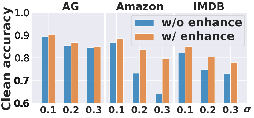
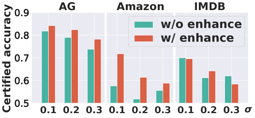
Figure 13: Accuracy w/ and w/o enhanced training on different $\sigma$ under LSTM. Right: clean accuracy. Left: certified accuracy against the SynonymInsert attack.

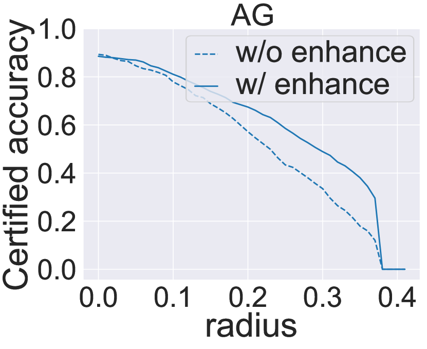
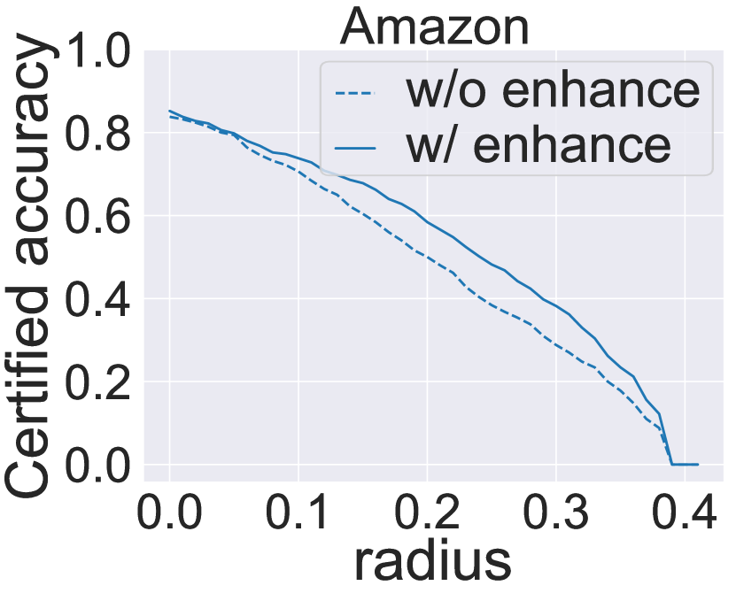
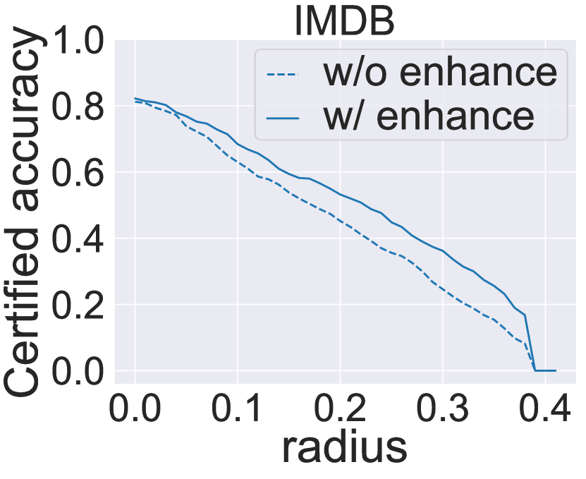
Figure 14: Certified accuracy at different radii w/ and w/o enhanced training on the noise level $\sigma=0.1$ under LSTM.

Table IX: Clean model accuracy under vanilla training (Clean vanilla) and under robust training (Clean Acc.).

Dataset (Model)	Clean vanilla	Noise	Clean Acc.
			Substitution	Reordering	Insertion	Deletion
AG (LSTM)		Low	90.12%	91.67%	90.38%	91.53%
	91.79%	Med.	89.59%	91.21%	86.66%	91.01%
		High	88.82%	91.40%	84.83%	90.38%
AG (BERT)		Low	93.24%	93.62%	93.43%	93.70%
	93.68%	Med.	92.75%	93.55%	93.05%	93.71%
		High	92.63%	93.43%	91.78%	93.51%
Amazon (LSTM)		Low	87.86%	88.59%	88.51%	88.71%
	89.82%	Med.	87.29%	88.44%	83.61%	88.62%
		High	86.23%	88.36%	79.53%	88.10%
Amazon (BERT)		Low	93.91%	94.11%	94.64%	94.73%
	94.35%	Med.	93.07%	94.27%	94.43%	94.49%
		High	91.62%	94.30%	92.89%	93.84%
IMDB (LSTM)		Low	83.39%	86.85%	84.86%	86.33%
	86.17%	Med.	82.58%	86.08%	80.45%	86.32%
		High	81.07%	86.11%	77.96%	84.76%
IMDB (BERT)		Low	91.52%	92.08%	91.88%	92.46%
	91.52%	Med.	90.42%	91.92%	91.68%	92.17%
		High	88.68%	91.99%	87.49%	90.55%

Table X: Attack accuracy of different real-world attacks.

Dataset (Model)	Text- Fooler[9]	Word Reorder[49]	Synonym Insert[50]	BAE- Insert[10]	Input Reduction[13]
AG (LSTM)	2.46%	76.38%	70.55%	-	40.85%
AG (BERT)	6.67%	49.36%	75.07%	28.53%	56.59%
Amazon(LSTM)	0.09%	54.16%	61.25%	-	30.85%
Amazon(BERT)	15.38%	5.29%	66.39%	9.30%	41.68%
IMDB (LSTM)	0.00%	40.20%	58.12%	-	30.65%
IMDB (BERT)	21.81%	7.54%	57.03%	18.66%	36.03%

References

- [1] “Chatgpt,” https://chat.openai.com/, developed by OpenAI.
- [2] Y. Zhang, S. Sun, M. Galley, Y.-C. Chen, C. Brockett, X. Gao, J. Gao, J. Liu, and W. B. Dolan, “Dialogpt: Large-scale generative pre-training for conversational response generation,” in ACL SD, 2020.
- [3] K. Shuster, D. Ju, S. Roller, E. Dinan, Y.-L. Boureau, and J. Weston, “The dialogue dodecathlon: Open-domain knowledge and image grounded conversational agents,” in ACL, 2020.
- [4] S. Roller, E. Dinan, N. Goyal, D. Ju, M. Williamson, Y. Liu, J. Xu, M. Ott, E. M. Smith, Y.-L. Boureau et al., “Recipes for building an open-domain chatbot,” in EACL, 2021.
- [5] A. Gramatzki, “9 text classification examples in action,” https://levity.ai/blog/9-text-classification-examples, 2022.
- [6] K. Ganesan, “Ai document classification: 5 real-world examples — opinosis analytics,” https://www.opinosis-analytics.com/blog/document-classification/, 2021.
- [7] S. Ren, Y. Deng, K. He, and W. Che, “Generating natural language adversarial examples through probability weighted word saliency,” in ACL, 2019.
- [8] R. Maheshwary, S. Maheshwary, and V. Pudi, “Generating natural language attacks in a hard label black box setting,” in AAAI, 2021.
- [9] D. Jin, Z. Jin, J. T. Zhou, and P. Szolovits, “Is bert really robust? a strong baseline for natural language attack on text classification and entailment,” in AAAI, 2020.
- [10] S. Garg and G. Ramakrishnan, “Bae: Bert-based adversarial examples for text classification,” in EMNLP, 2020.
- [11] D. Lee, S. Moon, J. Lee, and H. O. Song, “Query-efficient and scalable black-box adversarial attacks on discrete sequential data via bayesian optimization,” in ICML, 2022.
- [12] D. Li, Y. Zhang, H. Peng, L. Chen, C. Brockett, M.-T. Sun, and W. B. Dolan, “Contextualized perturbation for textual adversarial attack,” in NAACL HLT, 2021.
- [13] S. Feng, E. Wallace, A. Grissom II, P. Rodriguez, M. Iyyer, and J. Boyd-Graber, “Pathologies of neural models make interpretation difficult,” in EMNLP, 2018.
- [14] L. Wu, F. Morstatter, K. M. Carley, and H. Liu, “Misinformation in social media: definition, manipulation, and detection,” ACM SIGKDD explorations newsletter, 2019.
- [15] I. J. Goodfellow, J. Shlens, and C. Szegedy, “Explaining and harnessing adversarial examples,” in ICLR, 2015.
- [16] A. Madry, A. Makelov, L. Schmidt, D. Tsipras, and A. Vladu, “Towards deep learning models resistant to adversarial attacks,” in ICLR, 2018.
- [17] X. Dong, A. T. Luu, R. Ji, and H. Liu, “Towards robustness against natural language word substitutions,” in ICLR, 2021.
- [18] K. Yoo, J. Kim, J. Jang, and N. Kwak, “Detection of adversarial examples in text classification: Benchmark and baseline via robust density estimation,” in ACL, 2022.
- [19] M. Mozes, P. Stenetorp, B. Kleinberg, and L. Griffin, “Frequency-guided word substitutions for detecting textual adversarial examples,” in EACL, 2021.
- [20] X. Wang, J. Hao, Y. Yang, and K. He, “Natural language adversarial defense through synonym encoding,” in UAI, 2021.
- [21] Y. Yang, X. Wang, and K. He, “Robust textual embedding against word-level adversarial attacks,” in UAI, 2022.
- [22] J. Cohen, E. Rosenfeld, and Z. Kolter, “Certified adversarial robustness via randomized smoothing,” in ICML, 2019.
- [23] D. Zhang, M. Ye, C. Gong, Z. Zhu, and Q. Liu, “Black-box certification with randomized smoothing: A functional optimization based framework,” in NeurIPS, 2020.
- [24] L. Li, T. Xie, and B. Li, “Sok: Certified robustness for deep neural networks,” in SP. IEEE, 2022.
- [25] R. Jia, A. Raghunathan, K. Göksel, and P. Liang, “Certified robustness to adversarial word substitutions,” in EMNLP-IJCNLP, 2019.
- [26] C.-Y. Ko, Z. Lyu, L. Weng, L. Daniel, N. Wong, and D. Lin, “Popqorn: Quantifying robustness of recurrent neural networks,” in ICML, 2019.
- [27] T. Du, S. Ji, L. Shen, Y. Zhang, J. Li, J. Shi, C. Fang, J. Yin, R. Beyah, and T. Wang, “Cert-rnn: Towards certifying the robustness of recurrent neural networks,” in CCS, 2021.
- [28] G. Bonaert, D. I. Dimitrov, M. Baader, and M. Vechev, “Fast and precise certification of transformers,” in PLDI, 2021.
- [29] M. Ye, C. Gong, and Q. Liu, “Safer: A structure-free approach for certified robustness to adversarial word substitutions,” in ACL, 2020.
- [30] J. Zeng, X. Zheng, J. Xu, L. Li, L. Yuan, and X. Huang, “Certified robustness to text adversarial attacks by randomized [mask],” arXiv preprint arXiv:2105.03743, 2021.
- [31] H. Zhao, C. Ma, X. Dong, A. T. Luu, Z.-H. Deng, and H. Zhang, “Certified robustness against natural language attacks by causal intervention,” in ICML, 2022.
- [32] B. Wang, J. Jia, X. Cao, and N. Z. Gong, “Certified robustness of graph neural networks against adversarial structural perturbation,” in KDD, 2021.
- [33] M. Fischer, M. Baader, and M. Vechev, “Certified defense to image transformations via randomized smoothing,” in NeurIPS, 2020.
- [34] L. Li, M. Weber, X. Xu, L. Rimanic, B. Kailkhura, T. Xie, C. Zhang, and B. Li, “Tss: Transformation-specific smoothing for robustness certification,” in CCS, 2021.
- [35] M. Alfarra, A. Bibi, N. Khan, P. H. Torr, and B. Ghanem, “Deformrs: Certifying input deformations with randomized smoothing,” in AAAI, 2022.
- [36] Z. Hao, C. Ying, Y. Dong, H. Su, J. Song, and J. Zhu, “Gsmooth: Certified robustness against semantic transformations via generalized randomized smoothing,” in ICML, 2022.
- [37] H. Liu, J. Jia, and N. Z. Gong, “Pointguard: Provably robust 3d point cloud classification,” in CVPR, 2021.
- [38] P. Huang, Y. Yang, F. Jia, M. Liu, F. Ma, and J. Zhang, “Word level robustness enhancement: Fight perturbation with perturbation,” in AAAI, 2022.
- [39] Q. Geng, P. Kairouz, S. Oh, and P. Viswanath, “The staircase mechanism in differential privacy,” JSTSP, 2015.
- [40] J. Pennington, R. Socher, and C. D. Manning, “Glove: Global vectors for word representation,” in EMNLP, 2014.
- [41] J. Devlin, M.-W. Chang, K. Lee, and K. Toutanova, “BERT: Pre-training of deep bidirectional transformers for language understanding,” in NAACL, 2019.
- [42] “Bidirectional recurrent neural networks,” IEEE transactions on Signal Processing, vol. 45, no. 11, pp. 2673–2681, 1997.
- [43] Y. Kim, “Convolutional neural networks for sentence classification,” in EMNLP, 2014.
- [44] A. Vaswani, N. Shazeer, N. Parmar, J. Uszkoreit, L. Jones, A. N. Gomez, Ł. Kaiser, and I. Polosukhin, “Attention is all you need,” in NeurIPS, 2017.
- [45] J. Li, S. Ji, T. Du, B. Li, and T. Wang, “Textbugger: Generating adversarial text against real-world applications,” in NDSS, 2019.
- [46] J. Ebrahimi, A. Rao, D. Lowd, and D. Dou, “Hotflip: White-box adversarial examples for text classification,” in ACL, 2018.
- [47] J. Gao, J. Lanchantin, M. L. Soffa, and Y. Qi, “Black-box generation of adversarial text sequences to evade deep learning classifiers,” in SPW, 2018.
- [48] D. Pruthi, B. Dhingra, and Z. C. Lipton, “Combating adversarial misspellings with robust word recognition,” in ACL, 2019.
- [49] M. Moradi and M. Samwald, “Evaluating the robustness of neural language models to input perturbations,” in EMNLP, 2021.
- [50] J. Morris, E. Lifland, J. Y. Yoo, J. Grigsby, D. Jin, and Y. Qi, “Textattack: A framework for adversarial attacks, data augmentation, and adversarial training in nlp,” in EMNLP SD, 2020.
- [51] B. Wang, C. Xu, S. Wang, Z. Gan, Y. Cheng, J. Gao, A. H. Awadallah, and B. Li, “Adversarial glue: A multi-task benchmark for robustness evaluation of language models,” in NeurIPS, 2021.
- [52] M. Iyyer, J. Wieting, K. Gimpel, and L. Zettlemoyer, “Adversarial example generation with syntactically controlled paraphrase networks,” in NAACL-HLT, 2018.
- [53] M. T. Ribeiro, T. Wu, C. Guestrin, and S. Singh, “Beyond accuracy: Behavioral testing of nlp models with checklist,” in ACL, 2020.
- [54] M. Lecuyer, V. Atlidakis, R. Geambasu, D. Hsu, and S. Jana, “Certified robustness to adversarial examples with differential privacy,” in SP. IEEE, 2019.
- [55] J. Neyman and E. S. Pearson, “On the problem of the most efficient tests of statistical hypotheses,” Philosophical Transactions of the Royal Society of London, 1933.
- [56] H. Hong and Y. Hong, “Certified adversarial robustness via anisotropic randomized smoothing,” arXiv:2207.05327, 2022.
- [57] X. Zhang, J. Zhao, and Y. LeCun, “Character-level convolutional networks for text classification,” in NeurIPS, 2015.
- [58] J. McAuley and J. Leskovec, “Hidden factors and hidden topics: understanding rating dimensions with review text,” in RecSys, 2013.
- [59] A. Maas, R. E. Daly, P. T. Pham, D. Huang, A. Y. Ng, and C. Potts, “Learning word vectors for sentiment analysis,” in ACL HLT, 2011.
- [60] S. Hochreiter and J. Schmidhuber, “Long short-term memory,” Neural Comput., vol. 9, no. 8, p. 1735–1780, 1997.
- [61] D. Cer, Y. Yang, S.-y. Kong, N. Hua, N. Limtiaco, R. S. John, N. Constant, M. Guajardo-Cespedes, S. Yuan, C. Tar et al., “Universal sentence encoder,” arXiv preprint arXiv:1803.11175, 2018.
- [62] M. Alzantot, Y. S. Sharma, A. Elgohary, B.-J. Ho, M. Srivastava, and K.-W. Chang, “Generating natural language adversarial examples,” in EMNLP, 2018.
- [63] Y. Zang, F. Qi, C. Yang, Z. Liu, M. Zhang, Q. Liu, and M. Sun, “Word-level textual adversarial attacking as combinatorial optimization,” in ACL, 2020.
- [64] S. Tan, S. Joty, M.-Y. Kan, and R. Socher, “It’s morphin’time! combating linguistic discrimination with inflectional perturbations,” in ACL, 2020.
- [65] Y. Nie, Y. Wang, and M. Bansal, “Analyzing compositionality-sensitivity of nli models,” in AAAI, 2019.
- [66] Y. Yan, R. Li, S. Wang, F. Zhang, W. Wu, and W. Xu, “Consert: A contrastive framework for self-supervised sentence representation transfer,” in ACL, 2021.
- [67] H. Lee, D. A. Hudson, K. Lee, and C. D. Manning, “Slm: Learning a discourse language representation with sentence unshuffling,” in EMNLP, 2020.
- [68] M. Behjati, S.-M. Moosavi-Dezfooli, M. S. Baghshah, and P. Frossard, “Universal adversarial attacks on text classifiers,” in ICASSP, 2019.
- [69] Y. Xie, D. Wang, P.-Y. Chen, J. Xiong, S. Liu, and O. Koyejo, “A word is worth a thousand dollars: Adversarial attack on tweets fools stock prediction,” in NAACL HLT, 2022.
- [70] P.-S. Huang, R. Stanforth, J. Welbl, C. Dyer, D. Yogatama, S. Gowal, K. Dvijotham, and P. Kohli, “Achieving verified robustness to symbol substitutions via interval bound propagation,” in EMNLP, 2019.
- [71] J. C. Pérez, M. Alfarra, S. Giancola, B. Ghanem et al., “3deformrs: Certifying spatial deformations on point clouds,” in CVPR, 2022.
- [72] A. Bojchevski, J. Gasteiger, and S. Günnemann, “Efficient robustness certificates for discrete data: Sparsity-aware randomized smoothing for graphs, images and more,” in ICML, 2020.
- [73] S. Shalev-Shwartz et al., “Online learning and online convex optimization,” Foundations and Trends® in Machine Learning, vol. 4, no. 2, pp. 107–194, 2012.
- [74] D. E. Knuth, “Upper bound for binomial coefficient - proofwiki,” https://proofwiki.org/wiki/Upper_Bound_for_Binomial_Coefficient.