Grid Hopping: Accelerating Direct Estimation Algorithms for Multistatic FMCW Radar

Abstract

This paper presents a novel signal processing technique, coined grid hopping, as well as an active multistatic Frequency-Modulated Continuous Wave (FMCW) radar system designed to evaluate its performance. The design of grid hopping is motivated by two existing estimation algorithms. The first one is the indirect algorithm estimating ranges and speeds separately for each received signal, before combining them to obtain location and velocity estimates. The second one is the direct method jointly processing the received signals to directly estimate target location and velocity. While the direct method is known to provide better performance, it is seldom used because of its high computation time. Our grid hopping approach, which relies on interpolation strategies, offers a reduced computation time while its performance stays on par with the direct method. We validate the efficiency of this technique on actual FMCW radar measurements and compare it with other methods.

I Introduction

Multistatic radar systems are being increasingly used in multiple applications such as low-cost monitoring or automotive systems [1, 2, 3]. A multistatic radar is composed of one or more transmitter (TX) and at least two receivers (RXs) with widely spread locations. This enables the estimation of the location and velocity of one or multiple targets with an increased diversity by viewing the targets from different angles [4, 5, 6]. In this work, we developed an active K-band FMCW multistatic radar designed for detection of cars in civil applications. The focus of this paper is the comparison of the performance of different estimation algorithms by means of actual measurements. Moreover, we propose a novel processing methodology, called grid hopping, which appears as an efficient trade off between the computational complexity and the performance when compared to existing algorithms.

Conventional processing algorithms for multistatic radars can be classified into two categories. Indirect methods estimate ranges and speeds of the targets separately for each received signal. Then they combine the estimates to provide location and velocity estimates through multilateration. Direct methods, on the other hand, process all received signals jointly to directly estimate locations and velocities, commonly by maximizing a decision function evaluated over a grid of values [7, 8, 9]. In short, the indirect algorithms are faster as they require the evaluation of a few 2D Fast Fourier Transforms (FFT) that correspond to correlations in the range-Doppler domain. The direct algorithms require the discretization of the 4D location-velocity domain which makes them computationally heavier. Yet, the results of a direct processing are more robust to non-idealities.

Grid hopping is inspired by contributions for sound source localization applications [10, 11, 12]. In brief, we approximate the evaluation of the decision function used by the direct method with an interpolation performed on the output of the 2D FFT used in the indirect method. Thereby, the grid hopping enables us to keep the philosophy of the direct method with a computation time similar to the indirect method, and hence provides a compromise between the two strategies.

Notations: Vectors and matrices are denoted by lowercase and uppercase bold letters, respectively. Given a matrix $\boldsymbol{A}$, we use $\boldsymbol{A}^{*}$, $\boldsymbol{A}^{\top}$ and $\boldsymbol{A}[i]$ to respectively denote the conjugate, the transpose and the $i$-th row of $\boldsymbol{A}$. The scalar product and the outer product between two vectors respectively read $\langle\cdot,\,\cdot\rangle$ and $\otimes$. Finally $\mathrm{j}=\sqrt{-1}$.

II Radar Model

This section introduces the simplified model for the signals acquired by a multistatic FMCW radar. The model is similar to the one derived in [13]. The system uses a modulation made of linear chirps characterized by a carrier frequency $f_{0}$, and bandwidth $B$ and a chirp duration $T_{\mathrm{c}}$. A processed frame is composed of the acquisition of $M_{\mathrm{c}}$ chirps with $M_{\mathrm{s}}$ uniform samples per chirp. We restrict here the model to one target.

We consider a multistatic radar composed of one TX located in $\boldsymbol{x}^{\mathrm{TX}}$ and $Q$ RXs located in $\{\boldsymbol{x}^{\mathrm{RX}}_{q}\}_{q=1}^{Q}$. The whole system observes a scene that contains a single target assumed to be characterized by a single couple of location-velocity vectors ($\boldsymbol{x}$, $\boldsymbol{v}$), namely the parameters of interest. We consider subspaces $\mathcal{X}$ and $\mathcal{V}$ from which $\boldsymbol{x}$ and $\boldsymbol{v}$ are respectively known to be taken. Each receiver indexed by $q$ provides a signal that depends on the range and the radial speed of the target, respectively denoted by $r_{q}$ and $u_{q}$. Those are the sensed parameters and are defined with respect to the given receiver trough the sensing functions $S^{\mathrm{r}}_{q}$ and $S^{\mathrm{u}}_{q}$. These function are defined as

$$r_{q} =S^{\mathrm{r}}_{q}(\boldsymbol{x})=\textstyle\frac{2B}{{\sf c}}\,\big{(}\|\boldsymbol{x}-\boldsymbol{x}^{\mathrm{TX}}\|_{2}+\|\boldsymbol{x}-\boldsymbol{x}^{\mathrm{RX}}_{q}\|_{2}\big{)},$$ (1)

$$u_{q} =S^{\mathrm{u}}_{q}(\boldsymbol{x},\boldsymbol{v})=\textstyle\frac{2f_{0}T_{c}}{{\sf c}}\,\big{\langle}\frac{\boldsymbol{x}-\boldsymbol{x}^{\mathrm{TX}}}{\|\boldsymbol{x}-\boldsymbol{x}^{\mathrm{TX}}\|_{2}}+\frac{\boldsymbol{x}-\boldsymbol{x}^{\mathrm{RX}}_{q}}{\|\boldsymbol{x}-\boldsymbol{x}^{\mathrm{RX}}_{q}\|_{2}},\,\boldsymbol{v}\big{\rangle}.$$ (2)

The measurement provided by the $q$-th RXs is reshaped into a matrix denoted by $\boldsymbol{Y}_{q}\in\mathbb{C}^{M_{\mathrm{c}}\times M_{\mathrm{s}}}$ which can, under a few assumption described in [14, 15, 13], be written as

$$\textstyle\boldsymbol{Y}_{q}=\alpha_{q}\boldsymbol{b}(u_{q})\otimes\boldsymbol{a}(r_{q})+\boldsymbol{W}_{q},$$ (3)

where $\alpha_{q}\in\mathbb{C}$ is a scattering coefficient of amplitude and phase, and where $\boldsymbol{W}_{q}$ is a noise term. The functions $\boldsymbol{a}(r_{q})$ and $\boldsymbol{b}(u_{q})$ are waveforms or atoms whose $m$-th components are respectively given by $a_{m}(r_{q})=\exp({\mathrm{j}2\pi\,r_{q}\,m})$ and $b_{m}(u_{q})=\exp({\mathrm{j}2\pi\,u_{q}\,m})$.

III Direct and Indirect methods

We summarize now the two classes of existing strategies to recover $\boldsymbol{x}$ and $\boldsymbol{v}$ from the set of measurements $\{\boldsymbol{Y}_{q}\}_{q=1}^{Q}$, namely the indirect and the direct methods. The indirect method starts by computing the estimates $\hat{r}_{q}$ and $\hat{u}_{q}$ independently for each index $q$. This is done by maximizing the range-Doppler map obtained by computing the modulo of the 2D FFT of $\boldsymbol{Y}_{q}$. Then, the location $\boldsymbol{x}$ is estimated from $\hat{\boldsymbol{x}}^{\mathrm{Ind}}$, this quantity being computed by this multilateration

$$\hat{\boldsymbol{x}}^{\mathrm{Ind}}=\textstyle\arg\,\max_{\boldsymbol{x}^{\prime}\in\mathcal{X}}\sum_{q=1}^{Q}|S^{\mathrm{r}}_{q}(\boldsymbol{x}^{\prime})-\hat{r}_{q}|^{2}.$$ (4)

The velocity $\boldsymbol{v}$ is estimated similarly from $\{\hat{u}_{q}\}_{q=1}^{Q}$ and $S^{\mathrm{u}}_{q}$. Note that the computation time for (4) is negligible when compared to the computation time required for the $Q$ FFT s computed in the first step.

The direct algorithm works on grids discretizing the spaces $\mathcal{X}$ and $\mathcal{V}$ and denoted by respectively $\mathcal{X}_{\mathrm{G}}$ and $\mathcal{V}_{\mathrm{G}}$. The factorized methodology for the direct method that is used in [13] leads to

$$\hat{\boldsymbol{x}}^{\mathrm{Dir}}=\textstyle\arg\max_{\boldsymbol{x}\in\mathcal{X}_{\mathrm{G}}}\sum_{q=1}^{Q}\sum_{m_{\mathrm{c}}=1}^{M_{\mathrm{c}}}\big{|}\big{\langle}\boldsymbol{Y}_{q}[m_{\mathrm{c}}],\,\boldsymbol{a}(S^{\mathrm{r}}_{q}(\boldsymbol{x}))\big{\rangle}\big{|}^{2}$$ (5)

for the direct estimation of the location. Then, defining ${\boldsymbol{g}}_{q}=\boldsymbol{Y}^{*}\boldsymbol{a}(S^{\mathrm{r}}_{q}(\hat{\boldsymbol{x}}^{\mathrm{Dir}}))$, we compute the velocity estimate as

$$\hat{\boldsymbol{v}}^{\mathrm{Dir}}=\textstyle\arg\,\max_{\boldsymbol{v}\in\mathcal{V}_{\mathrm{G}}}\sum_{q=1}^{Q}|\langle{\boldsymbol{g}}_{q},\,\boldsymbol{a}(S^{\mathrm{u}}_{q}(\hat{\boldsymbol{x}}^{\mathrm{Dir}},\boldsymbol{v}))\rangle|^{2}.$$ (6)

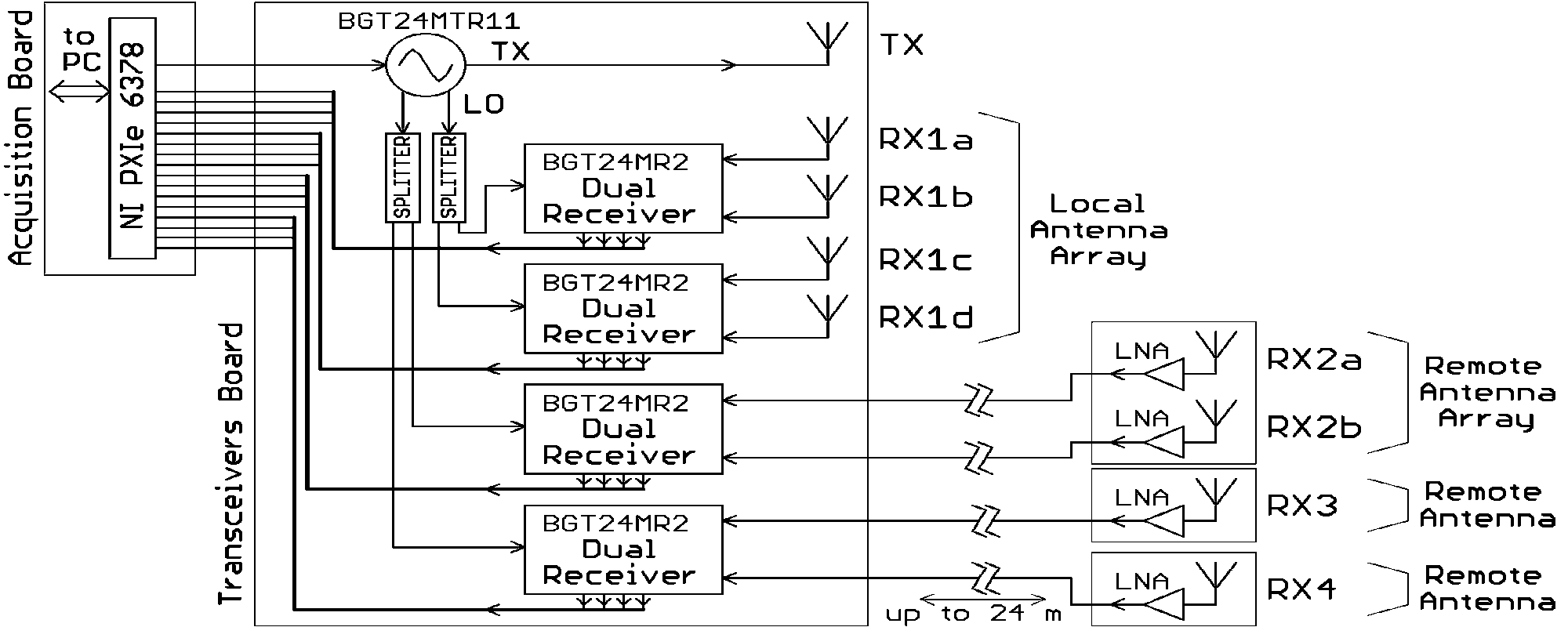
Figure 1: Simplified schematic representation of the hardware.

IV Grid Hopping

Our grid hopping technique relies on an interpolation strategy enabling the approximation of the scalar products on which relies the direct method. We formulate it for the estimation of location (5). Given a receiver index $q$ and a column $m_{\mathrm{c}}$, let us denote by $\boldsymbol{z}$ the output of the FFT of the column $\boldsymbol{Y}_{q}[m_{\mathrm{c}}]$. Then, the $i$-th component of $\boldsymbol{z}$ corresponds to the correlation between $\boldsymbol{Y}_{q}[m_{\mathrm{c}}]$ and $\boldsymbol{a}(\bar{r}_{i})$ where $\bar{r}_{i}$ is the $i$-th range taken from the grid of frequencies (and hence ranges) that is implicitly used by the FFT. The grid hopping aims at approximating the scalar products in (5) as follows. For all $\boldsymbol{x}^{\prime}\in\mathcal{X}_{\mathrm{G}}$, we identify a set of indexes $\mathcal{I}$ and a set of interpolation coefficients $\boldsymbol{c}$ such that

$$\langle\boldsymbol{Y}_{q}[m_{\mathrm{c}}]),\,\boldsymbol{a}(S^{\mathrm{r}}_{q}(\boldsymbol{x}^{\prime}))\rangle\simeq\boldsymbol{c}^{\top}\boldsymbol{z}_{\mathcal{I}},$$ (7)

where $\boldsymbol{z}_{\mathcal{I}}$ denotes the vector $\boldsymbol{z}$ restricted to the set of indexes $\mathcal{I}$. The quality of the approximation (7) is determined by both the interpolation method and the density of the frequency grid used in the FFT to obtain $\boldsymbol{z}$. In this paper, we use the polar interpolation whose efficiency has been demonstrated in Fourier atoms interpolation [16, 17, 18]. The computation of the interpolation coefficients for all $\boldsymbol{x}^{\prime}\in\mathcal{X}_{\mathrm{G}}$ is heavy but performed offline.

To apply grid hopping to the velocity estimation (6), we cannot compute the index sets and the coefficients offline; the speed sensing function $S^{\mathrm{u}}$ indeed depends on the location that must be first estimated. To avoid the online computation of interpolation coefficients, we use for the velocity estimation the simplest interpolation scheme where each set $\mathcal{I}$ contains a single index for all $\boldsymbol{v}^{\prime}\in\mathcal{V}_{\mathrm{G}}$.

To summarize, grid hopping follows the same principle as the direct method. Yet, the explicit scalar products required in (5) and (6) are replaced by an interpolation procedure such as (7). Indirect, direct and grid hopping strategies are compared hereafter.

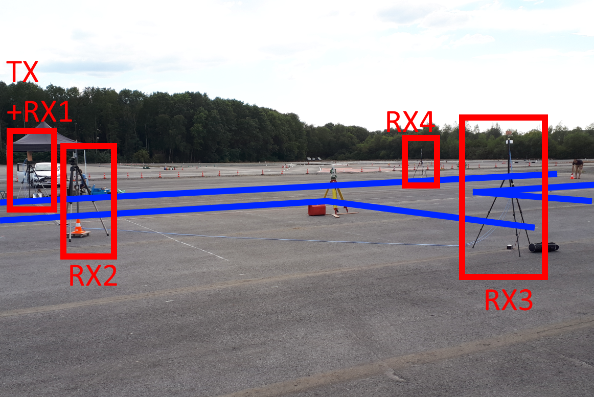
Figure 2: (left) Geometry of the system, showing the locations of the TX and the RXs. The axis depicts the 2D ground in meters. The dashed part of the car path is a portion that we discard from the measurement because the car was outside the sight of all receiving antennas. The dots and arrows are respectively the location and velocity estimates resulting from the hopping algorithms with grid densities of half the resolution. (right) Photo of the actual setup.

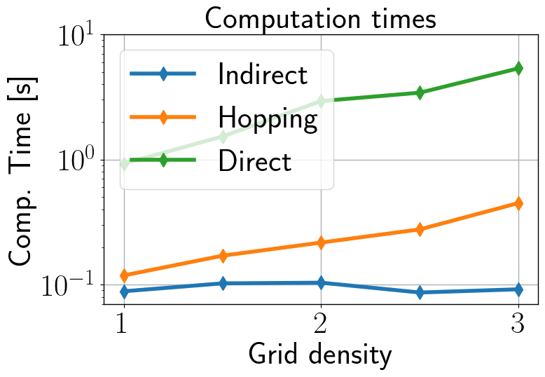
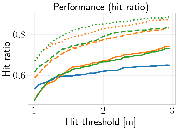
Figure 3: Computation time and performance comparison of the three algorithms. The hit ratio is the amount of hits divided by the total number of processed frames (433). (In right graph) Solid line : grid density $d=1$. Dashed : $d=2$, Dotted : $d=4$. A grid density $d$ means that the spacing between adjacent bins of $\mathcal{X}_{\mathrm{G}}$ is $1/d$ times the radar’s range resolution (60cm).

V Experimental results

To compare the three algorithms, we designed an active multistatic radar system and measured different scenarios with one to four cars moving along controlled patterns. The radar system is built around the BGT24 family of radio frequency transceivers from Infineon. Figure 1 shows a simplified schematic of the hardware. The base station includes a computer, the acquisition board, one transmitter and a four antennas array. Three remote stations are connected to the base station through coaxial cables of length up to 24 m, and are equipped with respectively a two antennas array, twice a single antenna. A general purpose data acquisition board (NI 6378 from National Instruments) outputs voltage ramps toward the voltage controlled oscillator (BGT24MTR11) to generate chirps of duration $T_{\mathrm{c}}=128\mu$s around $f_{0}=24GHz$, with $B=250MHz$. This signal feeds the TX antenna and is split to also feed all the RXs. The receivers are IQ demodulators (BGT24MR2) followed by baseband amplification and filtering circuits. The remote stations have a local low noise amplifier to compensate the losses in the cables. The baseband signals are sampled by the acquisition board such that $M_{\mathrm{s}}=M_{\mathrm{c}}=128$ and sent to the computer for processing.

This paper presents a first glimpse of the results. We focus on a scenario represented in Fig. 2 where a single car is moving along the path depicted in the figure. For simplicity, one RX antenna in each station was used for the processing presented in this paper. The radar signals were acquired for 60 seconds at a rate of one processed frame of $M_{\mathrm{c}}M_{\mathrm{s}}$ samples every 60ms on average. After discarding the frames where the car was outside the sight of all RXs, $433$ processed frames are left to assess the performances of the different algorithms.

The performance and the computation time of the three methods are compared in Fig. 3. Each location estimate resulting from each algorithm was compared to the approximated ground truth drawn in Fig. 2. As the car is not a single point in space, such comparison can only make sense with a tolerance threshold. When the error between an estimate and the reference is smaller than the “hit threshold”, we counted it as a hit (see Fig. 3). The performance was tested for multiple densities of $\mathcal{X}_{\mathrm{G}}$. We observe that the direct method performs better than the indirect one with a higher computational time. The hopping strategy provides an alternative with a computation time closer to the indirect method while exhibiting performance similar to the direct method.

VI Conclusion

In this paper, we presented a novel methodology, called grid hopping, as a trade-off between the direct and the indirect methods. The efficiency of grid hopping was evaluated on actual radar measurements. The comparison was restricted to a single interpolation scheme and to our most simple scenario with a single car moving. In the future, we will study the grid hopping to iterative direct algorithms enabling the detection of multiple targets. We will also compare multiple interpolation schemes.

References

- [1] J. Lin, Y. Li, W. C.Hsu, , and T. Lee, “Design of an fmcw radar baseband signal processing system for automotive application,” Leuzzi F., Ferilli S. (eds) Traffic Mining Applied to Police Activities. TRAP 2017. Advances in Intelligent Systems and Computing, vol. 5, no. 42, 01 2016.
- [2] S. Saponara and B. Neri, “Radar sensor signal acquisition and 3d fft processing for smart mobility surveillance systems,” 2016 IEEE Sensors Applications Symposium (SAS), pp. 1–6, 04 2016.
- [3] F. C. S. Capobianco, L. Facheris and S. Marinai, “Vehicle classification based on convolutional networks applied tofmcw radar signals,” Leuzzi F., Ferilli S. (eds) Traffic Mining Applied to Police Activities. TRAP 2017. Advances in Intelligent Systems and Computing, vol. 728, 03 2018.
- [4] A. M. Haimovich, R. S. Blum, and L. J. Cimini, “Mimo radar with widely separated antennas,” IEEE Signal Processing Magazine, vol. 25, no. 1, pp. 116–129, 2008.
- [5] P. Stinco, M. S. Greco, F. Gini, and M. L. Manna, “Non-cooperative target recognition in multistatic radar systems,” Radar, Sonar and Navigation, IET, vol. 8, no. 4, p. 396–405, Jan. 2013.
- [6] B. Sun, H. Chen, X. Wei, and X. Li, “Multitarget direct localization using block sparse bayesian learning in distributed mimo radar,” International Journal of Antennas and Propagation, vol. 2015, pp. 11–23, May 2015.
- [7] Y. Eldar, P. Kuppinger, and H. Bölcskei, “Block-sparse signals: Uncertainty relations and efficient recovery,” IEEE Transaction on Signal Processing, vol. 58, no. 6, pp. 3042 – 3054, Jul. 2010.
- [8] S. Gogineni and A. Nehorai, “Polarimetric mimo radar with distributed antennas for target detection,” IEEE Transactions on Signal Processing, vol. 58, no. 3, pp. 1689–1697, 2010.
- [9] C. Berger and J. Moura, “Noncoherent compressive sensing with application to distributed radar,” Annual Conference on Information Sciences and Systems, vol. 45, no. 4, pp. 1–6, Mar. 2011.
- [10] M. Cobos, A. Marti, and J. J. Lopez, “A modified srp-phat functional for robust real-time sound source localization with scalable spatial sampling,” IEEE Signal Processing Letters, vol. 18, no. 1, pp. 71–74, 2011.
- [11] M. Cobos, F. Antonacci, A. Alexandridis, A. Mouchtaris, and B. Lee, “A survey of sound source localization methods in wireless acoustic sensor networks,” Wireless Communications and Mobile Computing, vol. 2017, pp. 1–24, 08 2017.
- [12] T. Dietzen, E. De Sena, and T. van Waterschoot, “Low-complexity steered response power mapping based on nyquist-shannon sampling,” in 2021 IEEE Workshop on Applications of Signal Processing to Audio and Acoustics (WASPAA), 2021, pp. 206–210.
- [13] G. Monnoyer de Galland, T. Feuillen, L. Jacques, and L. Vandendorpe, “Sparsity-driven moving target detection in distributed multistatic fmcw radars,” in 2019 IEEE 8th International Workshop on Computational Advances in Multi-Sensor Adaptive Processing (CAMSAP), 2019, pp. 151–155.
- [14] H. Bao, “The research of velocity compensation method based on range-profile function,” International Journal of Hybrid Information Technology, vol. 7, pp. 49–56, 03 2014.
- [15] T. Feuillen, A. Mallat, and L. Vandendorpe, “Stepped frequency radar for automotive application: Range-doppler coupling and distortions analysis,” in MILCOM 2016 - 2016 IEEE Military Communications Conference, Nov 2016, pp. 894–899.
- [16] C. Ekanadham, D. Tranchina, and E. P. Simoncelli, “Recovery of sparse translation-invariant signals with continuous basis pursuit,” IEEE Transactions on Signal Processing, vol. 59, no. 10, pp. 4735–4744, Oct 2011.
- [17] K. Fyhn, H. Dadkhahi, and M. F. Duarte, “Spectral compressive sensing with polar interpolation,” in 2013 IEEE International Conference on Acoustics, Speech and Signal Processing, May 2013, pp. 6225–6229.
- [18] K. Fyhn, M. F. Duarte, and S. H. Jensen, “Compressive parameter estimation for sparse translation-invariant signals using polar interpolation,” IEEE Transactions on Signal Processing, vol. 63, no. 4, p. 870–881, Feb 2015.