Specification of MiniDemographicABM.jl:
A simplified agent-based demographic model
of the United Kingdom
(Version 1.3)

Abstract

This documentation specifies a simplified non-calibrated demographic agent-based model of the UK, a largely simplified version of the Lone Parent Model presented in [Gostoli and Silverman, 2020]. In the presented model, individuals of an initial population are subject to ageing, deaths, births, divorces and marriages throughout a simplified map of towns of the UK. The specification employs the formal terminology presented in [Elsheikh, 2023a]. The main purpose of the model is to explore and exploit capabilities of the state-of-the-art Agents.jl Julia package [Datseris et al., 2022] in the context of demographic modeling applications. Implementation is provided via the Julia package MiniDemographicABM.jl [Elsheikh, 2023b]. A specific simulation is progressed with a user-defined simulation fixed step size on a hourly, daily, weekly, monthly basis or even an arbitrary user-defined clock rate. The model can serve for comparative studies if implemented in other agent-based modelling frameworks and programming languages. Moreover, the model serves as a base implementation to be adjusted to realistic large-scale socio-economics, pandemics or immigration studies mainly within a demographic context.

1 Overview

In this and the following sections, a model example is introduced according to the specification terminology proposed in [Elsheikh, 2023a]. Although, the document attempts to demonstrate an example of a model specification in a stand-alone manner, it is definitely helpful for a reader not familiar with the employed terminology to consult the cited article for in-depth clarification.

This section provides a brief overview while detailed specification are provided in the following sections. The brief overview is attempted to be sufficient for a general understanding of the model. The later detailed sections are appropriate for reproducing or exploiting the implementation.

1.1 Description and aims

The model is concerned with a simplified demographic-only version of the lone parent model introduced in [Gostoli and Silverman, 2020]. The presented model evolves an initial artificial population of the UK through a combination of events: births, deaths, marriages, divorces and ageing. The main purpose of the model is to act as

• an experimental model for examining the capabilities of agent-based modeling libraries in the context of demographic modeling s.a. the Agents.jl package [Datseris et al., 2022]

• as a base for implementing further demographic-related case studies s.a. epidemiology or immigration among others

1.2 Formal overview

The specification of the model and its simulation process is basically established by describing the elements of tuple listed in Equation (22) in [Elsheikh, 2023a], namely:

$$<\alpha_{sim},\mathcal{F},\mathcal{M},\mathcal{M}^{t_{0}},\mathcal{E},\mathcal{A},\mathcal{A}^{t_{0}}>$$ (22)

with

• $\alpha_{sim}=(\Delta t,t_{0},t_{final},seed)^{T}$: simulation parameters, cf. Section 1.3

• $\mathcal{F}$: the set of employed population features, cf. Section 1.4

• $\mathcal{M}$: the given ABM model mathematical form, briefly overviewed in Section 1.5 and formulated in details in Section 2

• $\mathcal{E}$: the set of events, specified as

  $$\mathcal{E}=\{ageing,births,deaths,divorces,marriages\}$$ (1)

  where detailed specification of each event is provided in Section 4

• $\mathcal{A}$: the set of model assumptions that should not be violated are excessively summarized in Section 1.6

• $\mathcal{M}^{t_{0}}$ and $\mathcal{A}^{t_{0}}$ the initial model states at the initial simulation time $t_{0}$ together with the initial model assumptions are detailed in Section 3

1.3 Simulation parameters $\alpha_{sim}$

In version 1.1 of the package MiniDemographicABM.jl [Elsheikh, 2023b], Table 1 lists selected default values of the simulation parameters out of other possible values:

$\alpha_{x}$	default value	possible values
$t_{0}$	2020	the first of January of 1800-2020
$\Delta_{t}$	Daily	{Hourly, Daily, Monthly}
$t_{final}$	2030	the end of December of 2020-2100
$seed$	random	arbitrary

Table 1: Values of simulation parameters

linecolor=gray,backgroundcolor=gray!25,bordercolor=green]Comment: It is beneficial in future to further propose several case studies with specific simulation parameter values for each case.

1.4 Population features $\mathcal{F}$

The employed elementary population features are summarized Table 2.

Features	Predicates
age	$adult?$ ($~{}\equiv~{}\neg child?~{}\equiv~{}age\geq 18?$ ), $age=a?$
status	$alive?$, $female?$, $male?$, $orphan?$
	$marriageEligible?$, $married?$, $single?$
	$gaveBirth?$, $oldestSibling?$, $reproducible?$
space	$empty?$, $house$, $livesAlone?$
	$occupants$, $w?$ (i.e. in a town $w$)
kinship	$father$, $firstDegRelatives$, $mother$, $parents$
	$partner$, $youngestChild$, $wife$

Table 2: Set of employed elementary population features

1.5 The model $\mathcal{M}$ and its initial state $\mathcal{M}^{t_{0}}$

Equations (23) and (24) in [Elsheikh, 2023a]

$$\mathcal{M}\equiv\mathcal{M}^{t}\equiv\mathcal{M}(P(t),S(t),\alpha,D(t),t)$$ (23)

$$\text{ associated with }\mathcal{M}(P(t_{0}),S(t_{0}),\alpha,D(t_{0}),t_{0})=M^{t_{0}}$$ (24)

provide a brief description of the entities of the model where:

• $P\equiv P(t)$ corresponds to a population of individuals at time $t$

• The space

  $$S~{}\equiv~{}S(t)~{}=~{}<H(t)~{},~{}W>$$ (2)

  corresponds to a dynamic set of houses $H(t)$ distributed within a static set of towns $W$ of the UK, cf. Section 2.1 for detailed description

• model parameters $\alpha$ are provided in Section 2.2

• model input data $D$ is demonstrated in Section 2.3

• the initial model state $M^{t_{0}}$ is described in details in Section 3

1.6 Model assumptions $\mathcal{A}$ and initial assumptions $\mathcal{A}^{t_{0}}$

There are couple of distinguished subsets of assumptions:

• population-based assumptions (to be labeled with $a_{p}$)

• space-based assumptions (to be labeled with $a_{s}$)

• mixed (to be labeled with $a$) or

• initial assumptions $a^{0}$

A summary of all model assumptions is given in Table 3. Detailed possibly formal description of the assumptions are distributed throughout the documentation whenever relevant to the context.

label	summary	context
initial population related assumptions $a_{*}^{0}$
$a^{0}_{\ref{ass:init:adultsNoParents}}$	adults have no parents	Sec. 3.5
$a^{0}_{\ref{ass:init:childrenAliveParents}}$	parents are alive	”
$a^{0}_{\ref{ass:init:ArbitraryAgeDiffSiblings}}$	arbitrary age difference among siblings	”
$a^{0}_{\ref{ass:init:familyTogether}}$	family lives together	Sec. 3.6
space-related assumptions $a_{s_{*}}$
$a_{s{\ref{ass:space:staticTowns}}}$	static set of towns	Sec. 2.1
$a_{s{\ref{ass:space:inhabitable}}}$	a just created house remains forever	”
$a_{s{\ref{ass:space:dynamicSpace}}}$	dynamic space	”
$a_{s{\ref{ass:space:dynamicHouses}}}$	dynamic set of houses	”
$a_{s{\ref{ass:space:houseXYTown}}}$	town-xy-coordinate house location	”
$a_{s{\ref{ass:space:housingUniformLocations}}}$	town houses uniformly distributed	”
$a_{s{\ref{ass:space:selectOrCreateEmptyHouse}}}$	empty house selection (for new owners)	”
$a_{s{\ref{ass:space:houseInArbitraryTown}}}$	population density oriented town selection	”
population-related assumptions $a_{p_{*}}$
$a_{p{\ref{ass:pop:gender}}}$	equal gender ratio	Sec. 3.2 & 4.3
$a_{p{\ref{ass:pop:marrigeaAge}}}$	only adults are married	Sec. 3.4 & 4.6
$a_{p{\ref{ass:pop:marriedGivesBirth}}}$	only married non-old women give births	Sec. 3.5 & 4.3
$a_{p{\ref{ass:pop:adoption}}}$	no adoption for orphans	Sec. 4.4
mixed population-space related assumptions $a_{*}$
$a_{\ref{ass:mixed:homeless}}$	no homeless	Sec. 3.6
$a_{\ref{ass:mixed:numOfOccupants}}$	arbitrary number of occupants	”
$a_{\ref{ass:mixed:housingKinship}}$	flatmates are relatives	Sec. 4.1
$a_{\ref{ass:mixed:adultToOwnHouse}}$	new adults move out	Sec. 4.2
$a_{\ref{ass:mixed:deadHaveNoHouse}}$	deads leave their house	Sec. 4.4
$a_{\ref{ass:mixed:divorceMaleToOwnHouse}}$	divorced male moves out	Sec. 4.5
$a_{\ref{ass:mixed:marriedHousing}}$	housing assignment of new couple	Sec. 4.6

Table 3: Summary of model assumptions

2 The model $\mathcal{M}$

2.1 The space $S$

2.1.1 Space-related model assumptions $a_{s_{*}}$

Before diving into the specification of the space $S$, it makes sense to list some related set of space-oriented assumptions. The space $S$, cf. Equation (2) is composed of a tuple $<H(t)~{},~{}W>$ corresponding to the set of all houses $H(t)$ and towns $W$ implying that:

$a_{s{1}}$ The set of towns is constant during a simulation, i.e. no town vanishes nor new ones get constructed: $$\text{ if }t_{0}\leq t_{1}\neq t_{2}\leq t_{final}\implies W(t_{1})\equiv W(t_{2})\equiv W$$ (3)

$a_{s{2}}$ Once a new house is built (e.g. to host an adult moving out of his parent’s house), it never gets demolished and remains always inhabitable $$\text{ if }h\in H(t)~{}\implies h\in post(H(t))\text{ where }t_{0}\leq t<t_{final}$$ (4)

Based on the space definition and the previous Equation, the following assumption is considered:

$a_{s{3}}$ The space is not necessarily static and particularly the set of houses can vary along the simulation time span, i.e. $$\text{ if }t_{0}\leq t<t_{final}\implies H(t)\subseteq post(H(t))$$ (5)

Consequently,

$a_{s{4}}$ Each town $w\in W$ contains a dynamic set of of houses $$w(H^{t})\equiv H_{w}^{t}\equiv H_{w}(t)$$ (6)

2.1.2 The space $S$ – description

In the sake of simplifying the implementation of the space, the static set of towns of UK, cf. $a_{s{\ref{ass:space:staticTowns}}}$, is projected as a rectangular $12\times 8$ grid with each point in the grid corresponding to a town [Gostoli and Silverman, 2020]. Formally, assuming that

$$location(w_{(x,y)})=(x,y)$$

then

• the town $w_{(1,1)}$ corresponds to the north-est west-est town of UK whereas

• the town $w_{(12,8)}$ corresponds to the south-est east-est town of UK

• the distances between towns are commonly defined, e.g.

  $$\text{manhattan-distance}(w_{(x_{1},y_{1})},w_{(x_{2},y_{2})})=\mid x_{1}-x_{2}\mid+\mid y_{1}-y_{2}\mid$$ (7)

The (initial) population and houses distribution within UK towns are approximated by an ad-hoc pre-given UK population density map. The map is projected as a rectangular matrix

$$M\in R^{12\times 8}\approx\begin{bmatrix}0.0&0.1&0.2&0.1&0.0&0.0&0.0&0.0\\ 0.1&0.1&0.2&0.2&0.3&0.0&0.0&0.0\\ 0.0&0.2&0.2&0.3&0.0&0.0&0.0&0.0\\ 0.0&0.2&1.0&0.5&0.0&0.0&0.0&0.0\\ 0.4&0.0&0.2&0.2&0.4&0.0&0.0&0.0\\ 0.6&0.0&0.0&0.3&0.8&0.2&0.0&0.0\\ 0.0&0.0&0.0&0.6&0.8&0.4&0.0&0.0\\ 0.0&0.0&0.2&1.0&0.8&0.6&0.1&0.0\\ 0.0&0.0&0.1&0.2&1.0&0.6&0.3&0.4\\ 0.0&0.0&0.5&0.7&0.5&1.0&1.0&0.0\\ 0.0&0.0&0.2&0.4&0.6&1.0&1.0&0.0\\ 0.0&0.2&0.3&0.0&0.0&0.0&0.0&0.0\end{bmatrix}$$ (8)

It can be observed for instance that

• cells with density $0$ (i.e. realistically, with very low-population density) don’t correspond to inhabited towns

• the towns in UK are merged into 48 towns

• e.g. the center of the capital London spans the cells $(10,6),(10,7),(11,6)$ and $(11,7)$

2.1.3 Further space-related assumptions

Further assumptions are needed for specification of houses, their creation and their distributions within the UK:

$a_{s{5}}$ The static location of a house $h\in H^{[t,t_{final}]}_{w}$ is given in xy-coordinate of the town $$location(h)=(x,y)_{w}\text{ where }1\leq x,y\leq 25$$ (9)

$a_{s{6}}$ The locations of houses $H_{w}$ within a town $w\in W$ are uniformly distributed along the x- and y- axes $$Dist(location(H_{w}))\propto(U^{[1,25]},U^{[1,25]})$$ (10)

The previous equation reads the distribution is proportional to. Furthermore,

$a_{s{7}}$ If an empty house $h$ is demanded in a particular town $w\in W$, an empty house is randomly selected from the set of existing empty houses $H_{w(empty)}$ in that town $w$ $$h_{w}=random(H_{w(empty)})$$ (11) If no empty house exists, a new empty house is established according to assumptions $a_{s{\ref{ass:space:housingUniformLocations}}}$ and $a_{s{\ref{ass:space:houseXYTown}}}$

$a_{s{8}}$ If an empty house $h$ is demanded in an arbitrary town, a town is selected via a random weighted selection, say: $\displaystyle town(h)=random(W,M)$ (12) an empty house is selected or established according to the previous assumption

2.2 Model parameters $\alpha_{*}$

The following is a table of parameters employed for events specification, cf. Section 4. The values are set in an ad-hoc manner as they are not calibrated to actual data. The choice of data rather depends on the simulation parameters, e.g. the start and final simulation times, as well as the underlying case study.

$\alpha_{x}$	Value	Usage
$basicDivorceRate$	0.06	Equation 4.5
$basicDeathRate$	0.0001	Equation 4.4
$basicMaleMarriageRate$	0.7	Equation 4.6
$femaleAgeDeathRate$	0.00019	Equation 4.4
$femaleAgeScaling$	15.5	Equation 4.4
$initialPop$	10000	Section 3.1
$maleAgeDeathRate$	0.00021	Equation 4.4
$maleAgeScaling$	14.0	Equation 4.4
$maxNumMarrCand$	100	Sections 3.4 & 4.6
${startMarriedRatio}$	0.8	Equation 18

The value of the initial population size is just an experimental value and can be selected, for instance, from the set $\left\{10^{4},10^{5},10^{6},10^{7},10^{8}\right\}$ to examine the runtime performance of specific implementation and/or whether it is possible to enable a realistic demographic simulation with an actual population size.

2.3 Input data $D(t)$

In the archived Julia package MiniDemographicABM.jl [Elsheikh, 2023b], fertility data is given as:

$$D_{fertility}\in R^{35\times 360}~{}=$$

$$~{}~{}~{}~{}~{}\left[d_{ij}:\text{ fertility rate of women of age }i-16\text{ in year }j-1950\right]$$

This matrix, taken from the Python implementation of the Lone Parent Model [Gostoli and Silverman, 2020], reveals (the forecast of) the fertility rate for woman of ages 17 till 51 between the years 1951 and 2050, cf. Figure 1.

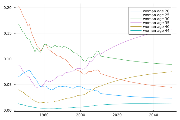
Figure 1: Fertility rates of women of different age classes between the years 1966 and hypothetically till 2310

Furthermore, the following (ad-hoc) data values, subject to tuning,:

$$D_{divorceModifierByDecade}\in R^{16}~{}=$$

$$~{}~{}~{}~{}~{}(0,1.0,0.9,0.5,0.4,0.2,0.1,0.03,0.01,0.001,0.001,0.001,0,0,0,0)^{T}$$

$$D_{maleMarriageModifierByDecade}\in R^{16}~{}=$$

$$~{}~{}~{}~{}~{}(0,0.16,0.5,1.0,0.8,0.7,0.66,0.5,0.4,0.2,0.1,0.05,0.01,0,0,0)^{T}$$

are employed in event specification, cf. Equations (4.5) and (4.6) for their contextual interpretation.

3 Model initialization $\mathcal{M}^{t_{0}}$

3.1 Initial population size and distribution $|P^{t_{0}}_{w}|$

The initial population size is given by the parameter $\alpha_{initialPop}$, cf. Section 2.2. The matrix $M$ and assumption $a_{s{\ref{ass:space:houseInArbitraryTown}}}$ provide together a stochastic ad-hoc estimate of the initial population distribution within the UK. That is, the initial population size of a town $w\in W$ is estimated as

$$|P_{w}(t_{0})|\approx\left\lceil\alpha_{initialPop}\times M_{y,x}/48\right\rceil\text{~{}~{} where ~{}~{}location}(w)=(x,y)$$ (13)

where 48 is the number of nonzero entries in $M$.

3.2 Gender $P^{t_{0}}=M^{t_{0}}\cup F^{t_{0}}$

The gender ratio distribution is specified via the following (clearly non-realistic) population-related assumption

$a_{p{1}}$ An individual can be equally a male or a female, i.e. $$Pr(p\in P^{t_{0}}_{male})\approx 0.5$$ (14)

This assumption is employed in the specification of the initial population as well as the specification of the birth event, cf. Section 4.3, and this it is not classified as an initial assumption.

3.3 Age distribution $P^{t_{0}}=\bigcup_{r}P_{age=r}^{t_{0}}$

The proposed non-negative age distribution of population individuals in years follows a normal distribution:

$$Dist\left(\frac{age(P^{t_{0}})}{N_{\Delta t}}\in\mathbb{Q}^{\alpha_{initialPop}}_{+}\right)~{}\propto~{}\left|\lfloor\mathcal{N}(0,\frac{100}{4}\cdot N_{\Delta t})\rfloor\right|$$ (15)

where $\mathbb{Q}_{+}$ stands for the set of positive rational numbers and $\mathcal{N}$ stands for a normal distribution with mean value 0 and standard deviation depending on

$$N_{\Delta t}~{}=~{}\left\{\begin{array}[]{ll}{}\dots\\ ~{}12&\text{ if }~{}\Delta t=month\\ 365&\text{ if }~{}\Delta t=day\\ 365\cdot 24&\text{ if }~{}\Delta t=hour\\ {}\dots\end{array}\right.$$ (16)

A possible outcome of the distribution of ages in an initial population of size 1,000,000 is shown in Figure 2.

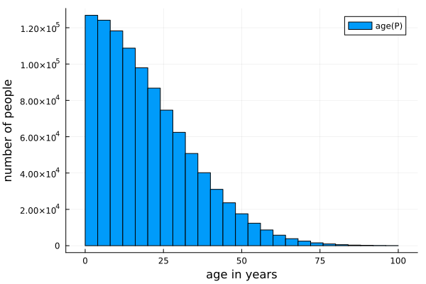
Figure 2: The distribution of ages in an initial population of size 1,000,000

Obviously, in reality, the shape of the age’s distribution depends on the initial simulation time $t_{0}$.

3.4 Partnership $P_{married}^{t_{0}}=M_{married}^{t_{0}}\cup partner(M_{married}^{t_{0}})$

Initially the following population assumption concerned with marriage age is considered

$a_{p{2}}$ A married person is an adult person $\displaystyle p\in P_{married}\implies age(p)\geq 18$ (17)

The ratio of married adults (males or females) is statistically approximated according to

$$Pr(p\in P_{isSingle~{}\cup~{}\neg adult}^{t_{0}})\approx 1-2\cdot\alpha_{startMarriedRatio}$$ (18)

That is, $\alpha_{startMarriedRate}$ is the ratio of married males (females) among adults. Partnership initialization is established according to Algorithm 1. Initially lines 1-3 initialize

1. the set of males randomly selected for marriage (line 1)

2. the set of females eligible to marriage (line 2)

3. and the number of female candidates for marriage each male has to select from (line 3).

For every male selected for marriage, a corresponding female is selected (lines 4-11):

1. a set of candidate females is initialized (line 5)

2. for every candidate female (line 6), a weight is calculated according to a weight function based on age difference in Equation (4.6) (line 7)

3. a female partner is selected according to a random weighted function (line 9)

4. the set of females illegible for marriage is updated (line 10)

Using the calculated weights, a partner

Algorithm 1 Partnership initialization

1: Select $M_{married}$ randomly according to Equation (18)

2:Set $F_{marriageEligible}^{t_{0}}=F_{marEli}^{t_{0}}=F_{adult~{}\cap~{}single}^{t_{0}}$

3:Set $n_{candidates}=max\left(\alpha_{maxNumMarrCand}~{},~{}\frac{|F_{marEli}|}{10}\right)$

4:for $m\in M_{married}$ do

5:     Set $F_{candidates}=random(F_{marEli},n_{candidates})$

6:     for $f\in F_{candidates}$ do

7:          Set $w_{m,f}=weight(m,f)=ageFactor(m,f)$ where

$$ageFactor(m,f)=~{}$$

$$~{}~{}~{}\left\{\begin{array}[]{ll}~{}1/(age(m)-age(f)-5+1)&\text{ if }~{}age(m)-age(f)\geq 5\\ ~{}-1/(age(m)-age(f)+2-1)&\text{ if }~{}age(m)-age(f)\leq-2\\ ~{}1\text{ ~{}~{}~{}~{}otherwise }\\ \end{array}\right.$$ (22)

8:     end for

9:     Set

$$f_{partner(m)}=weightedSample(F_{candidates},W_{m})$$

$$~{}~{}~{}~{}~{}\text{ where }~{}W_{m}=\left\{w_{i}:w_{i}=weight(m,f_{i})~{},~{}f_{i}\in F_{marEli}\right\}$$ (23)

10:     Set $F_{marEli}=F_{marEli}-\{f_{partner(m)}\}$

11:end for

3.5 Children and parents

The following assumptions are assumed only in the context of the initial population:

$a^{0}_{1}$ All adult persons have no parents $$p\in P_{age\geq 18}^{t_{0}}\implies\nexists q\in P^{t_{0}}\text{ s.t.\ }q\in parents(p)$$ (24)

$a^{0}_{2}$ All children have alive parents, i.e. $$p\in P_{age<18}^{t_{0}}\implies parents(p)\subset P_{alive}^{t_{0}}$$ (25)

Based on the previous two assumptions, one can may also deduce that there is no individual in the initial population who has a grandpa or grandma.

$a^{0}_{3}$ There is no age difference restriction among siblings, i.e. age difference can be less than 9 months

Moreover, the following population assumption proposes conditions for women who can give birth:

$a_{p{3}}$ Only a married female under age of 45 gives birth $\displaystyle f\in$ $\displaystyle F_{just(gaveBirth)}^{t}\implies$ $\displaystyle f\in F_{married}^{t}\text{ and }age(f)<45$ (26)

Assumptions $a_{p{\ref{ass:pop:marriedGivesBirth}}}$ and $a_{p{\ref{ass:pop:marrigeaAge}}}$ imply that only an adult person can become a parent. Children are assigned to married couples as parents in the following way. For any child $c\in P_{age<18}^{t_{0}}$, the set of potential fathers is established as follows:

$$M_{candidates}=~{} \{~{}m\in M_{married}\text{ s.t.\ }$$

$$min\left(~{}age(m),age(wife(m))~{}\right)\geq age(c)+18+\frac{9}{12}\text{ and }$$

$$age(wife(m))<45+age(c)~{}\}$$ (27)

out of which a random father is selected for the child:

$$father(c)= random(M_{candidates})\text{ and }$$

$$mother(c)=wife(father(c))$$

3.6 Housing assignments

Before specifying the housing assignments to initial population, related model assumptions are listed:

$a_{1}$ There are no homeless individuals: $$\text{ if }p\in P^{t}_{alive}~{}\implies~{}house(p^{t})\in H(t)$$ (28)

The last line in the previous equations indicates that a dead person does not need to be associated to any house. Furthermore, there is no classification of houses according to their capacities:

$a_{2}$ A house can be occupied by an arbitrary number of individuals

Moreover, the following assumption is considered for housing association:

$a^{0}_{4}$ A family, i.e. a married male and female, and their children live together, that is $\displaystyle|occupants(h^{t_{0}})|>1$ $\displaystyle\text{ with }p,q\in occupants(h^{t_{0}})\text{ and }p\neq q~{}\implies~{}$ $\displaystyle p\in firstDegRelatives(q)$ (29)

The previous assumption implies that a single person in the initial population shall be assigned a house alone. The assignment of newly established houses to initial population considers the assumptions $a_{s{\ref{ass:space:selectOrCreateEmptyHouse}}}$ and $a_{s{\ref{ass:space:houseInArbitraryTown}}}$. That is, the location of new houses in $H(t_{0})$ is specified according to to Equation (12), each is assigned to a single person or a family as previously stated.

4 Events

This section provides compact algorithmic specification of events serving as a comprehensive demonstration of the proposed terminology presented in [Elsheikh, 2023a].

4.1 Execution order of events

Despite Equation (1) specifying the set of events, the considered events are just alphabetically listed without enforcing a certain appliance order, except for the ageing event which should proceed any other events. That is,

$$e_{1}=ageing$$

This is reasonable since if an event s.a. death or birth proceeds ageing, then this implies that the population size and features may not remain consistent with input data $D(t)$, model parameters $\alpha$ and initial model states $\mathcal{M}^{t_{0}}$.

The execution order of the rest of the events as well as the order of the agents subject to such events, whether sequential or random, remains an implementation detail. Nevertheless, since many of the events are following a random stochastic process, probably, the higher the resolution of the simulation becomes (e.g. weekly step-size instead of monthly, or daily instead of weekly), the less influential the execution order of the events becomes.

The combination of event transitions on the population does not preserve the initial assumption $a^{0}_{\ref{ass:init:familyTogether}}$ regarding the occupants of houses. Therefore, assumption regarding the occupants of houses is further relaxed to:

$a_{3}$ Any two individuals living in a single house are either a 1-st degree relatives, step-parent, step-child, step-siblings or partners. An exception to the previous assumption occurs when an orphan’s oldest sibling is married in which case they also lives together as a family.

4.2 Ageing

The ageing process of a population can be described as follows:

$$ageing\left(P_{alive(age=a)}^{t}\right)=P_{alive(age=a+\Delta t)}^{t+\Delta t}~{}~{},~{}~{}\forall a\in\{0,\Delta t,2\Delta t,...\}$$ (30)

That is, the age of any individual as long as he remains alive is incremented by $\Delta t$ for each simulation step. Furthermore, the following assumption concerned with individuals becoming adults is considered:

$a_{4}$ In case a teenager becomes an adult and he/she is not the oldest orphan, he/she gets re-allocated to an empty house in the same town.

Formally:

$$ageing \left(P_{alive(age=18-\Delta t)~{}\cap~{}\neg\left(orphan~{}\cap~{}oldestSibling\right)}\right)=$$

$$P_{alive(age=18)~{}\cap~{}livesAlone}$$ (31)

Moreover,

$$\text{If }p\in P^{t}_{alive(age=18)}\implies town(p)=pre(town(p))$$ (32)

The re-allocation to an empty house should be according to assumption $a_{s{\ref{ass:space:selectOrCreateEmptyHouse}}}$.

4.3 Births

For simplification purpose, from now on, it is implicitly assumed (unless specified) that only the alive population is involved in event-based transition of population features. Given assumption 3.5, let the set of reproducible females be defined as:

$$F_{reproducible} ~{}=~{}F_{married~{}\cap~{}age<45}~{}\bigcap~{}$$

$$F_{age(youngestChild)>1~{}\cup~{}\neg hasChildren}$$ (33)

That is, the set of all married females in a reproducible age and either do not have children or those with youngest child older than one. The birth event produces new children from reproducible females specified as follows

$$birth \left(F^{t}_{reproducible}\right)~{}=~{}$$

$$~{}\left(F_{reproducible}^{t+\Delta t}~{}-~{}F_{just(reproducible)}^{t+\Delta t}\right)~{}\bigcup$$

$$~{}F_{just(\neg reproducible)}^{t+\Delta t}~{}\bigcup$$

$$~{}P_{age=0}^{t+\Delta t}$$ (34)

The previous equation states that the birth event transients the individuals within the set of reproducible females to:

• those females who remained reproducible (first line in the rhs)

• those who just gave births (second line) and

• new neonates are produced (third line)

Note that the following set is subtracted from those who remained reproducible

$$F_{just(reproudicble)}~{}=~{}F_{just(married)}~{}\cup~{}F_{married(age(youngestChild)=1)}$$ (35)

and (given Assumption $a_{p{\ref{ass:pop:marriedGivesBirth}}}$) those who became non-reducible include also who got divorced and widowed

$$F_{just(\neg reproducible)}~{}=~{}$$

$$~{}~{}~{}F_{age(youngestChild)=0}~{}\cup~{}F_{just(\neg married)}~{}\cup~{}F_{married(age=45)}$$ (36)

Employing assumptions $a_{\ref{ass:mixed:housingKinship}}$ and $a_{\ref{ass:mixed:adultToOwnHouse}}$, one can deduce that a neonate is assigned to his parents house, i.e.

$$p\in~{} P_{age=0}\implies$$

$$house(p)=house(mother(p))$$ (37)

The yearly-rate of births produced by the sub-population $F_{reproducible,(age=a)}^{t}$ i.e. reproducible females of age $a$ years old with actual simulation time $t$, depends on the yearly-basis fertility rate data:

$$R_{birth,yearly}(F_{reproducible,(age=a)}^{t})~{}\propto~{}D_{fertility}(a-16,currentYear(t))$$ (38)

This implies that the instantaneous probability that a reproducible female $f\in F_{reproducible}^{t}$ gives birth to a new individual $p\in P^{t+\Delta t}_{age=0}$ depends on $D_{fertility}(a-16,currentYear(t))$ and is given by Equation (57), cf. Appendix A for a conceptual review regarding rates and instantaneous probabilities.

4.4 Deaths

The death event transforms a given population of alive individuals as follows:

$$death\left(P_{alive}^{t}\right)~{}=~{}P_{alive-age=0}^{t+\Delta t}~{}\bigcup~{}P_{just(\neg alive)}^{t+\Delta t}$$ (39)

where

• the first phrase in the right hand side stands for the alive population except neonates as they don’t belong to $P^{t}_{alive}$

• the second phrase stands for those who just became dead

The following simplification assumptions are considered:

$a_{p{4}}$ No adoption or parent re-assignment to orphans is established after their parents die $\displaystyle p\in P_{child}\text{ and }parents(p)$ $\displaystyle\subset P_{\neg alive}\implies$ $\displaystyle post(parents(p))\subset P_{\neg alive}$ (40)

$a_{5}$ Those who just became dead they leave their houses, i.e. $\displaystyle\text{ if }p\in P_{just(\neg alive)}^{t+\Delta t}~{}$ $\displaystyle\text{ and }~{}pre(house(p))=h$ $\displaystyle\implies~{}$ $\displaystyle p\notin P^{t+\Delta t}_{h}~{}\text{ and }~{}house(p)\notin H^{t+\Delta t}$ (41)

Note that $P_{h}$ stands for the population (or occupants) of a house $h$. The amount of population deaths depends on the yearly-rate given by:

$$R_{death,yearly} (p\in P)=\alpha_{basicDeathRate}~{}+~{}$$

$$\left\{\begin{array}[]{cc}\left(e^{\frac{age(p)}{\alpha_{maleAgeScaling}}}\right)\times\alpha_{maleAgeDeathRate}\text{ if }male?(p)\\ \left(e^{\frac{age(p)}{\alpha_{femaleAgeScaling}}}\right)\times\alpha_{femaleAgeDeathRate}\text{ if }female?(p)\\ \end{array}\right.$$ (44)

from which instantaneous probability of the death of an individual is derived as illustrated in Appendix A.

4.5 Divorces

The divorce event causes that a subset of married population becomes divorced:

$$divorce(M_{married}^{t})~{}=~{}$$

$$~{}~{}~{}~{}~{}M_{married-just(married)}^{t+\Delta t}~{}\bigcup~{}M_{just(isDivorced)}^{t+\Delta t}$$ (45)

The first phrase in the right hand side refers to the set of married individuals who remained married excluding those who just got married. The second phrase refers to the population subset who just got divorced in the current iteration. Note that it is sufficient to only apply the divorce event to either the male or female sub-populations. After divorce takes place, the housing’s assignment is specified according to the following assumption:

$a_{6}$ Any male who just got divorced moves to an empty house within the same town (in conformance with Assumption $a_{s{\ref{ass:space:selectOrCreateEmptyHouse}}}$): $\displaystyle m\in$ $\displaystyle M_{just(isDivorced}^{t})\implies$ $\displaystyle pre(location(m))\neq location(m)~{}\text{ and }~{}livesAlone(m)~{}\text{ and }~{}$ $\displaystyle town(m)=pre(town(m))$ (46)

The re-allocation to an empty house is in conformance with assumption $a_{s{\ref{ass:space:selectOrCreateEmptyHouse}}}$. The amount of yearly divorces in married male populations can be estimated upon the yearly divorce rate given by

$$R_{divorce,yearly}(m\in M_{single}^{t}) ~{}=~{}$$

$$\alpha_{basicDivorceRate}~{}\cdot~{} D_{divorceModifierByDecade}(\lceil age(m)/10\rceil)$$ (47)

That is, the instantaneous probability of a divorce event to a married man $m\in M_{married}$ depends on $D_{divorceModifierByDecade}(\lceil age(m)/10\rceil)$, cf. Equation (57).

4.6 Marriages

Similar to the divorce event, it is sufficient to apply the marriage event to a sub-population of single males. Assuming that

$$M_{marEli}~{}=~{}M_{marriageEligible}~{}=~{}M_{single~{}\cup~{}age\geq 18}$$ (48)

the marriage event updates the state of few individuals within a sub-population to married males, formally:

$$marriage(M_{marEli}^{t})~{}=~{}$$

$$~{}~{}~{}~{}~{}M_{marEli-just(isDivorced)-age=18}^{t+\Delta t}~{}\bigcup~{}M_{just(married)}^{t+\Delta t}$$ (49)

The amount of yearly marriages can be statistically estimated by

$$R_{marraige,yearly}(m\in M_{single}^{t})~{}=~{}$$

$$~{}\alpha_{basicMaleMarriageRate}~{}\cdot~{}D_{maleMarriageModifierByDecade}(\lceil age(m)/10\rceil)$$ (50)

from which simulation-relevant instantaneous probability is calculated as given in Equation (57). For an arbitrary just married male $m\in M_{just(married)}^{t+\Delta t}$, his wife was selected according to a slight modification of Algorithm 1. Namely line 7 is modified to:

$$weight(m,f)~{}=~{}$$

$$~{}~{}~{}geoFactor(m,f)~{}\cdot~{}childrenFactor(m,f)~{}\cdot~{}ageFactor(m,f)$$ (51)

and

$$geoFactor(m,f)=~{}$$

$$~{}~{}~{}~{}~{}1/e^{(4\cdot\text{manhattan-distance}(town(m),town(f)))}$$ (52)

$$childrenFactor(m,f)=~{}$$

$$~{}~{}~{}~{}~{}1/e^{|children(m)|}\cdot 1/e^{|children(f)|}\cdot e^{|children(m)|\cdot|children(f)|}$$ (53)

Where $ageFactor(m,f)$ is given in Equation (7). Note that the just married male and his female partner don’t then belong to the set of marriage eligible population $P_{marEli}^{t+\Delta t}$. linecolor=gray,backgroundcolor=gray!25,bordercolor=green]Comment: It is thinkable to reverse the genders in the algorithm The following assumption specifies the housing’s assignment of the new couple.

$a_{7}$ When two individuals get married, the wife and the occupants of actual house (i.e. children and non-adult orphan siblings) moves to the husband’s house unless there are fewer occupants in his house. In the later case, the husband and the occupants of his house move to the wife’s house.

Formally, suppose that $m\in P^{t+\Delta t}_{just(married)}$ if

$$|P_{house(m^{t})}|\geq |P_{house(f^{t})}|\implies house(p^{t+\Delta t})=house(m),~{}\forall p^{t}\in P_{house(f^{t})}$$

Otherwise

$$house(p^{t+\Delta t})=house(f),~{}\forall p^{t}\in P_{house(m^{t})}$$ (54)

Appendix A Events rates and instantaneous probability

Pre-given data, e.g. mortality and fertility rates, are usually given in the form of finite rates (i.e. cumulative rate) normalized by sub-population length. In other words, the rate

$$R_{event,period(t,t+\Delta t)}(X^{t})~{},~{}X^{t}\subseteq P^{t}$$

corresponds to the number of occurrences that a certain $event$ within a sub-population $X$ (e.g. marriage) takes place in the time range between $(t,t+\Delta t)$, e.g. a daily, weekly, monthly or yearly rate, etc. normalized by the sub-population length. That is, say if a pre-given typically yearly rate is given as input data:

$$R_{event,yearly}(X^{t})~{}=~{}D_{event,yearly}\in R^{N\times M}$$ (55)

where $M$ corresponds to a given number of years and $N$ corresponds to the number of particular features of interest, for examples:

• $M=100$ for mortality or fertility yearly rate data between the years 1921 and 2020

• $N=28$ for fertility rate data for women of ages between 18 and 45 years old, i.e. $28=45-18+1$

The yearly probability that an event takes place for a particular individual $x^{t}\in X^{t}$ is:

$$Pr_{event,yearly}(x^{t}\in X^{t})~{}=~{}D_{event,yearly}(yearsold(x^{t}),currentYear(t))$$ (56)

Pre-given data in such typically yearly format desires adjustments in order to employ them within a single clocked agent-based-model simulation of a fixed step size typically smaller than a year. Namely, the occurrences of such events need to be estimated at equally-distant time points with the pre-given constant small simulation step size $\Delta t$. For example, if we have population of 1000 individuals with a (stochastic) monthly mortality rate of $0.05$, then after

• one month (about) 50 individuals die with 950 left (in average)

• two months, about $902.5$ individuals are left

• $\dots$

• one year, 540 individuals are left resulting in a yearly finite rate of $0.46$

linecolor=gray,backgroundcolor=gray!25,bordercolor=green]Comment: may be a figure linecolor=gray,backgroundcolor=gray!25,bordercolor=green]Comment: better example based on daily rate , e.g. daily rate of 0.001 for a population of 1000 Typically mortality rate in yearly forms of various age classes are given, but a daily or monthly estimate of the rates shall be applied within an agent-based simulation.

The desired simulation-adjusted probability is approximated by rather evaluating the desired rate per very short period regardless of the simulation step-size, assumed to be reasonably small (e.g. hourly, daily, weekly or monthly at maximum). Formally, the so called instantaneous probability is evaluated as follows:

$$Pr_{event,instantaneous}(x^{t}\in X^{t},\Delta t)~{}=~{}-\frac{ln(1-Pr_{event,yearly}(x^{t}))}{N_{\Delta t}}$$ (57)

where $N_{\Delta}$ is given as in Equation (16).

Funding

Dr. Atyiah Elsheikh is a Research Software Engineer at MRC/CSO Social & Public Health Sciences Unit, School of Health and Wellbeing, University of Glasgow. He is in the Complexity in Health programme. He is supported by the Medical Research Council (MC_UU_00022/1) and the Scottish Government Chief Scientist Office (SPHSU16).

For the purpose of open access, the author(s) has applied a Creative Commons Attribution (CC BY) licence to any Author Accepted Manuscript version arising from this submission.

References

- [Datseris et al., 2022] Datseris, G., Vahdati, A. R., and DuBois, T. C. (2022). Agents.jl: A performant and feature-full agent-based modeling software of minimal code complexity. SIMULATION.
- [Elsheikh, 2023a] Elsheikh, A. (2023a). Formal specification terminology for demographic agent-based models of fixed-step single-clocked simulations. Technical report, arXiv.
- [Elsheikh, 2023b] Elsheikh, A. (2023b). MiniDemographicABM.jl: A simplified agent-based demographic model of the UK. CoMSES Computational Model Library. V1.1.1.
- [Gostoli and Silverman, 2020] Gostoli, U. and Silverman, E. (2020). Social and child care provision in kinship networks: An agent-based model. PLOS ONE, 15(12).