An Overconstrained Vertical Darboux Mechanism

Abstract

In this article, we will construct an overconstrained closed-loop linkage consisting of four revolute and one cylindrical joint. It is obtained by factorization of a prescribed vertical Darboux motion. We will investigate the kinematic behaviour of the obtained mechanism, which turns out to have multiple operation modes. Under certain conditions on the design parameters, two of the operation modes will correspond to vertical Darboux motions. It turns out, that for these design parameters, there also exists a second assembly mode.

1 Introduction

In 1881, Darboux determined all possible motions with the property, that every point has a planar trajectory. Vertical Darboux motions are a sub-type of these motions and are obtained by the composition of a rotation with a suitably parametrized oscillating translation in the direction of the rotation axis. All generic point trajectories for both the non-vertical and the vertical Darboux motion are ellipses. The vertical Darboux motion is in addition a cylindrical and line symmetric motion. For more detail we refer to [1, Chapter 9].

Vertical Darboux motions are of particular interest, when using Study parameters for the representation of spatial displacements. Any line in the ambient space of the Study quadric represents a vertical Darboux motion [8]. Lines on the Study quadric correspond to rotations and translations. Therefore the vertical Darboux motion is a natural generalization of rotations and translations. By representing the motion by a curve on the Study quadric,its instantaneous behaviour corresponds to the instantaneous motion given by the curve tangent, which is a line in the ambient space. Thus, vertical Darboux motions may also be used for the description of the instantaneous behaviour of a motion.

In this article, we construct an overconstrained $4$RC-linkage performing an arbitrary vertical Darboux motion. The construction is based on the factorization theory for dual quaternion polynomials [2] and on the construction of a non-vertical Darboux linkage in [6]. Lines on the Study quadric can be parametrized by linear dual quaternion polynomials, thus they represent rotations or translations. Both motions can easily be realized by revolute or prismatic joints, respectively. Thus, by decomposing a dual quaternion polynomial into the product of linear factors, we are able to construct open kinematic chains. For the vertical Darboux motion, we obtain an open chain, which can perform a cylindrical motion. Therefore, it can be closed using a cylindrical joint to obtain a single-loop mechanism.

Overconstrained mechanisms performing a vertcal Darboux motion are constructed in [3, 4]. Our approach, however, yields a new type of overconstrained mechanisms. We will analyze operation and assembly modes of the obtained linkage. In general, they will have two operation modes, one of them is the desired vertical Darboux motion, the other is a cylindrical motion of degree 5. Further, we will give a condition, which ensures existence of a second assembly mode, as well as the decompositon of the second operation mode into another vertical Darboux motion and two rotations.

2 Preliminaries

In this manuscript, we will construct a closed-loop linkage able to perform a vertical Darboux motion. Our construction is based on the factorizaton theory of dual quaternion polynomials, therefore we will give a short introduction to dual quaternions and motion polynomials in this section. For further detail we refer to [5].

2.1 Dual Quaternions

A dual quaternion $h\in\mathbb{DH}$ is given by

$$h=p_{0}+p_{1}\mathbf{i}+p_{2}\mathbf{j}+p_{3}\mathbf{k}+d_{0}\varepsilon+d_{1}\varepsilon\mathbf{i}+d_{2}\varepsilon\mathbf{j}+d_{3}\varepsilon\mathbf{k}$$

for real numbers $p_{0},\ldots,p_{3}$, $d_{0},\ldots,d_{3}\in\mathbb{R}$. The non-commutative multiplication of dual quaternions abides by the rules

$$\mathbf{i}^{2}=\mathbf{j}^{2}=\mathbf{k}^{2}=\mathbf{i}\mathbf{j}\mathbf{k}=-1,\quad\varepsilon^{2}=0,\quad\varepsilon\mathbf{i}=\mathbf{i}\varepsilon,\quad\varepsilon\mathbf{j}=\mathbf{j}\varepsilon,\quad\varepsilon\mathbf{k}=\mathbf{k}\varepsilon.$$

The quaternions $p=p_{0}+p_{1}\mathbf{i}+p_{2}\mathbf{j}+p_{3}\mathbf{k}$, $d=d_{0}+d_{1}\mathbf{i}+d_{2}\mathbf{j}+d_{3}\mathbf{k}$ are called primal and dual part of $h$. The dual quaternion conjugate is given by

$${h}^{\ast}=p_{0}-p_{1}\mathbf{i}-p_{2}\mathbf{j}-p_{3}\mathbf{k}+d_{0}\varepsilon-d_{1}\varepsilon\mathbf{i}-d_{2}\varepsilon\mathbf{j}-d_{3}\varepsilon\mathbf{k},$$

the dual quaternion norm is given by $\left\|h\right\|=h{h}^{\ast}$. Dual quaternions can be used to represent rigid body displacements by simply using the Study parameters of a displacement as the coefficients of the dual quaternion. The action of a displacement on a point $[x_{0},x_{1},x_{2},x_{3}]$ in projective three-space can be represented by a dual quaternion product by embedding the point into the dual quaternions via $[x_{0},x_{1},x_{2},x_{3}]\mapsto x_{0}+\varepsilon x$ with $x=x_{1}\mathbf{i}+x_{2}\mathbf{j}+x_{3}\mathbf{k}$. Acting on this point by a displacement given by $p+\varepsilon d$ corresponds to computing the product

$$(p-\varepsilon d)(x_{0}+\varepsilon x)({p}^{\ast}+\varepsilon{d}^{\ast}).$$

The coefficients of a dual quaternion $h$ fulfill the Study condition if and only if $\left\|h\right\|$ is real. Note that all scalar multiples of a dual quaternion yield the same displacement.

2.2 Motion Polynomials

Rational motions can be represented by polynomials with dual quaternion coefficients $Q=\prod_{\ell=0}^{n}q_{\ell}t^{\ell}$ with $q_{0}$, $q_{1},\ldots,q_{n}\in\mathbb{DH}$ such that $\left\|Q\right\|=Q{Q}^{\ast}\in\mathbb{R}[t]$ is a real polynomial. Here the conjugate polynomial ${Q}^{\ast}$ is obtained by conjugating all of its coefficients. Such polynomials are called motion polynomials.

The simplest examples of motion polynomials are linear, monic polynomials $t-h$, where the scalar coefficient $d_{0}$ of the dual part has to vanish for the Study condition to be fulfilled. Such a linear polynomial either represents a rotation, if $\left\|t-h\right\|$ has complex roots, or a translation otherwise. In case of a rotation, its axis has Plücker coordinates $[p_{1},p_{2},p_{3},-d_{1},-d_{2},-d_{3}]$. Otherwise the direction of translation is given by $[d_{1},d_{2},d_{3}]\in\mathbb{R}^{3}$. Both of these motions can be realized by revolute or prismatic joints, respectively. Decomposing a given motion polynomial into the product of linear factors therefore corresponds to decomposing the represented motion into a concatenation of rotations and translations, which in turn can be realized by joints. This gives rise to a kinematic chain which is able to perform the given motion. It can be constrained by another chain generated by a different factorization of the same motion polynomial, which yields a closed mechanism still able to perform the given motion.

3 Vertical Darboux Motion

A vertical Darboux motion is the composition of a rotation and an oscillating translation along the same axis. Vertical Darboux motions around the third coordinate axis can be parameterized by the dual quaternion polynomial [5].

$$M=(t^{2}+1)(t-\mathbf{k})+\varepsilon(-b\mathbf{k}t+c\mathbf{k})(t-\mathbf{k}).$$

It does not admit a factorization into three linear factors, but multiplying $M$ with $(t^{2}+1)$ allows us to find factorizations, each consisting of 5 linear polynomials [7]. Every factorization corresponds to an open kinematic chain with at most five revolute joints, which can perform the vertical Darboux motion given by $M$. Combining several of these chains would result in a rather complicated mechanism. But since the vertical Darboux motion is a cylindrical motion, we can close the obtained open chain with a C-joint. This results in a closed-loop mechanism with at most six joints where one of the joints has two degrees of freedom. To obtain an overconstrained mechanism, we can try to find factorizations for which two neighboring factors are equal. This yields an open $4$R chain which can be close with a C-joint resulting in an overconstrained mechanism.

3.1 Factorization of the vertical Darboux motion

Like in [6, Section 3.3], we will try to find $P_{4}\in\mathbb{DH}[t]$ such that $P_{4}^{2}$ is a right factor of $(t^{2}+1)M$. Solving a system of equations for the coefficients of $P_{4}$ shows that it has to be of the shape

$$P_{4}=t-k-\varepsilon(q_{1}\mathbf{i}+q_{2}\mathbf{j})$$

for arbitrary $q_{1}$, $q_{2}\in\mathbb{R}$. After dividing off these two right factors, we obtain

$$Q=(t^{2}+1)(t+\mathbf{k})+\varepsilon(bt-c+2t(q_{1}t+q_{2})\mathbf{i}-2t(q_{2}t+q_{1})\mathbf{j}-t(bt-c)\mathbf{k}),$$

which represents a Darboux motion. As long as $q_{1}$ and $q_{2}$ do not vanish simultaneously, it is non-vertical, thus admits infinitely many factorizations into three linear factors. Using factorization techniques, it is straight forward to compute

$$P_{3}=t+\mathbf{k}+\varepsilon(y_{1}\mathbf{i}+y_{2}\mathbf{j}),$$

which is a right factor of $Q$. Dividing off this factor will leave us with a quadratic translation, which admits a factorization if and only if it is a circular translation [5]. To ensure factorizability, we need to choose

$$y_{1} =\frac{b^{2}q_{1}-2bcq_{2}-c^{2}q_{1}+4q_{1}^{3}+4q_{1}q_{2}^{2}}{4(q_{1}^{2}+q_{2}^{2})},$$

$$y_{2} =\frac{b^{2}q_{2}+2bcq_{1}-c^{2}q_{2}+4q_{1}^{2}q_{2}+4q_{2}^{3}}{4(q_{1}^{2}+q_{2}^{2})}.$$

The resulting motion is then a translation along a circle with axis in the direction $[4(bq_{1}-cq_{2}),4(bq_{2}+cq_{1}),-b^{2}-c^{2}+4q_{1}^{2}+4q_{2}^{2}]$. To find a factorization for this translation, we can simply take any line parallel to the circle axis and use its normalized Plücker coordinates as the coefficients of the right factor, i.e. we can define

$$P_{2}=t+\frac{4(bq_{1}-cq_{2})\mathbf{i}+4(bq_{2}+cq_{1})\mathbf{j}-(b^{2}+c^{2}-4q_{1}^{2}-4q_{2}^{2})\mathbf{k}}{b^{2}+c^{2}+4q_{1}^{2}+4q_{2}^{2}}-\varepsilon(z_{1}\mathbf{i}+z_{2}\mathbf{j}+z_{3}\mathbf{k})$$

for $z_{1}$, $z_{2}$, $z_{3}\in\mathbb{R}$ such that the Study (Plücker) condition is fulfilled. After dividing off $P_{2}$ we are left with the last factor which is given by

$$P_{1}=t -\frac{4(bq_{1}-cq_{2})\mathbf{i}+4(bq_{2}+cq_{1})\mathbf{j}-(b^{2}+c^{2}-4q_{1}^{2}-4q_{2}^{2})\mathbf{k}}{b^{2}+c^{2}+4q_{1}^{2}+4q_{2}^{2}}$$

$$+\varepsilon\frac{2q_{2}\left(bc+2q_{1}q_{2}+2z_{1}q_{2}\right)-q_{1}\left(b^{2}-c^{2}-4q_{1}^{2}-4q_{1}z_{1}\right)}{4q_{1}^{2}+4q_{2}^{2}}\mathbf{i}$$

$$-\varepsilon\frac{2q_{1}\left(bc-2q_{1}q_{2}-2q_{1}z_{2}\right)+q_{2}\left(b^{2}-c^{2}-4q_{2}^{2}-4q_{2}z_{2}\right)}{4q_{1}^{2}+4q_{2}^{2}}\mathbf{j}$$

$$+\varepsilon\frac{4(bq_{1}-cq_{2})z_{1}+4(bq_{2}+cq_{1})z_{2}-b(b^{2}+c^{2}-4q_{1}^{2}-4q_{2}^{2})}{b^{2}+c^{2}-4q_{1}^{2}-4q_{2}^{2}}\mathbf{k}$$

assuming ${b^{2}+c^{2}-4q_{1}^{2}-4q_{2}^{2}}\neq 0$. Note, that $z_{3}$ is chosen such that the Study condition for $P_{2}$ is fulfilled.

If ${b^{2}+c^{2}-4q_{1}^{2}-4q_{2}^{2}}=0$, $z_{3}$ can be chosen arbitrarily, with the restriction that $z_{1}$ and $z_{2}$ need to fulfill $[z_{1},z_{2}]=z[bq_{2}+cq_{1},-bq_{1}+cq_{2}]$ for arbitrary $z\in\mathbb{R}$. With this condition, the last factor is given by

$$P_{1}=t -2\frac{(bq_{1}-cq_{2})\mathbf{i}+(bq_{2}+cq_{1})\mathbf{j}}{b^{2}+c^{2}}$$

$$-\varepsilon\frac{(b^{2}+c^{2})z-2c}{b^{2}+c^{2}}((bq_{2}+cq_{1})\mathbf{i}-(bq_{1}-cq_{2})\mathbf{j})$$

$$+\varepsilon(z_{3}-b)\mathbf{k}.$$

This factorization

$$(t^{2}+1)M=P_{1}P_{2}P_{3}P_{4}^{2}$$

now gives rise to a $4$R chain, which we can close with a cylindrical joint to obtain a closed-loop linkage, see Fig, 1. It admits, by construction, the initial vertical Darboux motion given by $M$ as one operation mode.

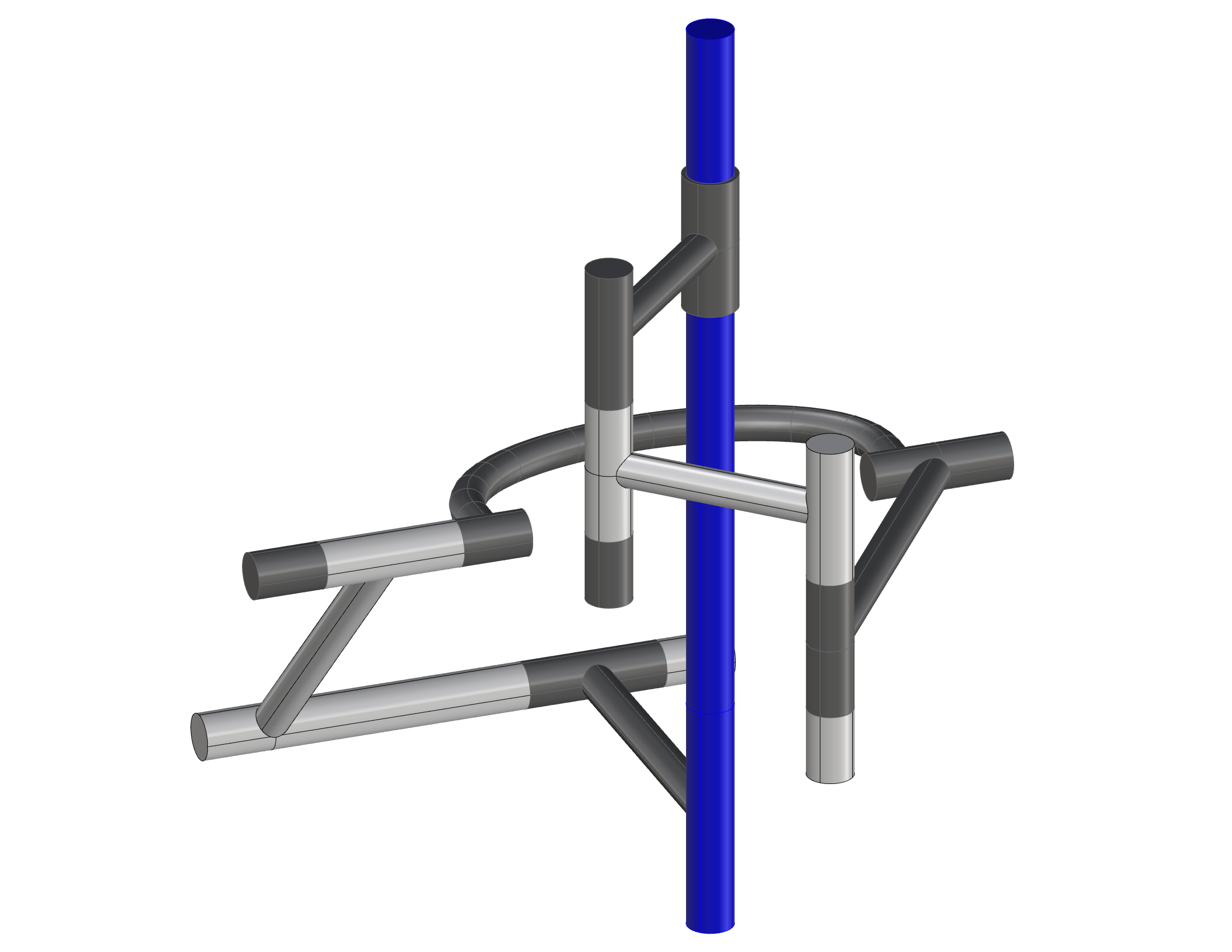
Figure 1: An example of a 4RC vertical Darboux mechanism (C-joint is blue).

4 Kinematic Analysis of the Vertical Darboux Mechanism

To analyze other possible operation modes, let us investigate the kinematic chain obtained by these factors, where each joint can move inepenently of each other, i.e. $C=P_{1}(v_{1})P_{2}(v_{2})P_{3}(v_{3})P_{4}(v_{4})(\tau-k)(1-\varepsilon s\mathbf{k})$. Here the last two factors simply describe a cylindrical joint with the third coordinate axis as joint axis. A kinematic chain can be closed, if the third coordinate axes of the base and the moving frame coincide. This yields two closure conditions, the first one being, that the axes point in the same direction, the second one, that they point in opposite directions.

4.1 First Assembly Mode

The first closure condition means that the coefficients of the dual quaternion units $\mathbf{i}$, $\mathbf{j}$, $\mathbf{k}$, $\varepsilon$, $\varepsilon\mathbf{i}$, $\varepsilon\mathbf{j}$ and $\varepsilon\mathbf{k}$ of $C$ vanish, i.e. $C$ describes the identity transformation. This gives us seven polynomial equations, where the first and the second have a common factor $v_{1}-v_{2}$ while the other factors do not have common real solutions. After substituting this into our set of equations, the third equation has the factor $\tau v_{3}-\tau v_{4}+v_{3}v_{4}+1$ while last equation has the factor $sv_{1}^{2}+bv_{1}-c+s$. They admit the real solution $s=-(bv_{2}-c)/(v_{1}^{2}+1)$, $\tau=-(v_{3}v_{4}+1)/(v_{3}-v_{4})$. After substituting these solutions into the remaining equations, we are left with two polynomial equations which are quadratic in each of the variables $v_{1}$, $v_{3}$ and $v_{4}$. Computing a resultant to eliminate $v_{4}$ and dividing off unnecessary factors yields an equation with two factors, one of them is $v_{1}-v_{3}$, the other

$$F= 8bcq_{1}^{2}v_{1}^{3}v_{3}+8bcq_{2}^{2}v_{1}^{3}v_{3}+b^{4}v_{1}^{3}-b^{4}v_{1}^{2}v_{3}+2b^{2}c^{2}v_{1}^{3}-2b^{2}c^{2}v_{1}^{2}v_{3}+4b^{2}q_{1}^{2}v_{1}^{3}$$

$$+12b^{2}q_{1}^{2}v_{1}^{2}v_{3}+4b^{2}q_{2}^{2}v_{1}^{3}+12b^{2}q_{2}^{2}v_{1}^{2}v_{3}+c^{4}v_{1}^{3}-c^{4}v_{1}^{2}v_{3}-4c^{2}q_{1}^{2}v_{1}^{3}$$

$$-12c^{2}q_{1}^{2}v_{1}^{2}v_{3}-4c^{2}q_{2}^{2}v_{1}^{3}-12c^{2}q_{2}^{2}v_{1}^{2}v_{3}-24bcq_{1}^{2}v_{1}^{2}-24bcq_{1}^{2}v_{1}v_{3}$$

$$-24bcq_{2}^{2}v_{1}^{2}-24bcq_{2}^{2}v_{1}v_{3}+v_{1}b^{4}-b^{4}v_{3}+2v_{1}c^{2}b^{2}-2b^{2}c^{2}v_{3}-12b^{2}q_{1}^{2}v_{1}$$

$$-4b^{2}q_{1}^{2}v_{3}-12b^{2}q_{2}^{2}v_{1}-4b^{2}q_{2}^{2}v_{3}+v_{1}c^{4}-c^{4}v_{3}+12c^{2}q_{1}^{2}v_{1}+4c^{2}q_{1}^{2}v_{3}$$

$$+12c^{2}q_{2}^{2}v_{1}+4c^{2}q_{2}^{2}v_{3}+8bcq_{1}^{2}+8bcq_{2}^{2}$$ (1)

This, in general, gives rise to two sets of solutions, the first one being $v_{3}=v_{1}$ which in turn also yields $v_{4}=(v_{1}^{2}-1)/2v_{1}$. This solution corresponds to the initial vertical Darboux motion.

The second solution is obtained by solving $F$ for $v_{3}$ as it is linear in this variable and resubstituting the obtained solution into the system of equations. This yields two equations with a common factor linear in $v_{4}$ and each of them has one other factor, respectively, which do not have a common solution provided $b^{2}+c^{2}-4q_{1}^{2}-4q_{2}^{2}\neq 0$ (this case will be investigated below). This common factor yields the solutions

$$v_{3} =\frac{v_{1}(v_{1}^{2}+1)(b^{2}+c^{2})^{2}+\left((b^{2}-c^{2})(v_{1}^{3}-3v_{1})-6bcv_{1}^{2}+2bc\right)(4q_{1}^{2}+4q_{2}^{2})}{(v_{1}^{2}+1)(b^{2}+c^{2})^{2}-((b^{2}-c^{2})(3v_{1}^{2}-1)+2bcv_{1}^{3}-6bcv_{1})(4q_{1}^{2}+4q_{2}^{2})}$$

$$v_{4} =-\frac{(bv_{1}+cv_{1}+b-c)(bv_{1}-cv_{1}-b-c)}{2(cv_{1}+b)(bv_{1}-c)}.$$

This solution corresponds to a motion with trajectories of degree six. It is the composition of the vertical Darboux motion given by

$$(t^{2}+1)(bt-c-(ct+b)\mathbf{k})+\varepsilon(bt-c)(ct+b+(bt-c)\mathbf{k})$$

and a quadratically parametrized rotation around the third coordinate axis

$$-(bt-2ct-b)(b^{2}+c^{2}+4q_{1}^{2}+4q_{2}^{2})+(ct^{2}+2bt-c)(b^{2}+c^{2}-4q_{1}^{2}-4q_{2}^{2})\mathbf{k}.$$ (2)

Figure 2 (left) shows a trajectory of the vertical Darboux motion (first solution) and this other motion (second solution) for the values $q_{1}=1$, $q_{2}=0$, $z_{1}=0$, $z_{2}=0$.

Let us now investigate the case, where $b^{2}+c^{2}-4q_{1}^{2}-4q_{2}^{2}=0$. With this condition the factor $F$ in Eq. (1) of the resultant simplifies to

$$F=(bv_{1}^{2}-2cv_{1}-b)(cv_{1}v_{3}+bv_{1}+bv_{3}-c).$$

The second factor yields the same solutions as in the case above. The first factor, however, gives rise to two additional sets of solutions

$$v_{1}=\frac{c\pm\sqrt{b^{2}+c^{2}}}{b},\qquad v_{4}=\frac{c}{b}.$$

Both of these solutions correspond to rotations around the third coordinate axis given by

$$2(c\sqrt{b^{2}+c^{2}}\pm(b^{2}+c^{2}))(ct+b-(bt-c)\mathbf{k})-\varepsilon b^{2}\sqrt{b^{2}+c^{2}}(bt-c+(ct+b)\mathbf{k}).$$

Further, the polynomial in Eq. (2) simplifies to a real polynomial, which implies, that the second solution in this special case also corresponds to a vertical Darboux motion. The trajectories of all of these motions are depicted in Figure 2 (right).

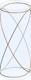
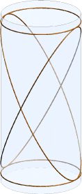
Figure 2: Trajectories of the coupler motion for $b=1$, $c=2$ and $b=c=\sqrt{2}$.

4.2 Second Assembly Mode

For the second closure condition, the dual quaternion coefficients of $1$, $\mathbf{k}$, $\varepsilon$, $\varepsilon\mathbf{i}$, $\varepsilon\mathbf{j}$, $\varepsilon\mathbf{k}$ need to vanish, while the coefficients of $\mathbf{i}$ and $\mathbf{j}$ must fulfill a linear equation. This corresponds to assembling the open kinematic chain such that the third coordinate axes of the base and moving frame coincide, but they point in opposite directions. For the linear condition of the coefficients $c_{i}$ and $c_{j}$ of $\mathbf{i}$ and $\mathbf{j}$ we will use the equation $(bq_{1}-cq_{2})c_{i}+(bq_{2}+cq_{1})c_{j}=0$ which will be the second equation in our closure condition.

Solving the first equation for $v_{2}$ and substituting the result into the third equation yields an equation which simplifies, after dividing off unnecessary factors, to $b^{2}+c^{2}-4q_{1}^{2}-4q_{2}^{2}=0$. Thus, this second assembly mode only exists, if this condition is fulfilled. Note that this condition is the same as in the section above for the existence of four operation modes in the first assembly.

In this case, the first, second and third equation only have one common solution for $v_{2}$ and $\tau$, namely

$$v_{2}=-1/v_{1},\qquad\tau=(v_{3}-v_{4})/(v_{3}v_{4}+1).$$

After resubstituting these solutions, equations five and six have one common factor which is linear in $s$ while their other factors do not admit common solutions. The solution for $s$ is

$$s=\frac{z(b^{2}+c^{2})(v_{1}^{2}+1)+2bv_{1}-2c}{2(v_{1}^{2}+1)}.$$

After resubstituting this solution, the last equation, after dividing off unnecessary factors, reads

$$(bv_{4}-c)(v_{3}^{2}-2v_{3}v_{4}-1)=0.$$ (3)

The first factor in Eq. (3) yields the two solutions

$$v_{1}=\frac{-c\pm\sqrt{-3b^{2}+8bz_{3}+c^{2}-4z_{3}^{2}}}{b-2z_{3}},\qquad v_{4}=\frac{c}{b}.$$

For the second factor in Eq. (3) we get $v_{4}=(v_{3}^{2}-1)/2v_{3}$. Resubstituting this solution yields the equation

$$-v_{1}^{2}v_{3}^{2}z_{3}+cv_{1}^{2}v_{3}+cv_{1}v_{3}^{2}+bv_{1}^{2}+bv_{3}^{2}-v_{1}^{2}z_{3}-v_{3}^{2}z_{3}+cv_{1}+cv_{3}+2b-z_{3}=0$$

This equation is quadratic in $v_{1}$ (and $v_{3}$), thus solving it for $v_{1}$ will yield two solutions.

In contrast to the first assembly mode, all solutions depend on $z$ and $z_{3}$, but not on $q_{1}$ and $q_{2}$. Further they contain square roots, thus the solutions can be complex. On the left hand side of Fig. 3 the trajectories of a point under these motions are shown for $b=c=\sqrt{2}$, $z=z_{3}=0$. For these values, only the second operation mode admits real trajectories. On the right hand side of Fig. 3, the trajecories for $b=1$, $c=2$, $z=z_{3}=0$ are shown. Here, also the first two solutions are real and the corresponding motions are rotations around the third coordinate axis.

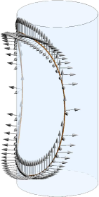
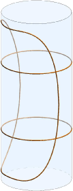
Figure 3: Coupler motion where the first two solutions are complex (left) or real (right).

5 Conclusion

We have generated an overconstrained 4RC closed-loop linkage, which is able to perform a prescribed vertical Darboux motion. Its kinematic analysis revealed the existence of, in general, two operation modes, one of them corresponding to the initial vertical Darboux motion. We gave a condition on the design parameters of the mechanism for which the second operation mode decomposes into two rotations and an additional vertical Darboux motion. The same condition also ensures the existence of a second assembly mode, which in turn has up to three real operation modes.

References

- [1] O. Bottema and B. Roth. Theoretical Kinematics. Dover Publications, 1990.
- [2] Gábor Hegedüs, Josef Schicho, and Hans-Peter Schröcker. Factorization of rational curves in the Study quadric and revolute linkages. Mech. Mach. Theory, 69(1):142–152, 2013.
- [3] Chung-Ching Lee and Jacques M. Hervé. On the vertical Darboux motion. In Jadran Lenarcic and Manfred Husty, editors, Latest Advances in Robot Kinematics, pages 99–106, Dordrecht, 2012. Springer Netherlands.
- [4] Chung-Ching Lee and Jacques M. Hervé. Vertical Darboux motion and its parallel mechanical generators. Meccanica, 50(12):3103–3118, 2015.
- [5] Z. Li, , T. Rad, J. Schicho, and H.-P. Schröcker. Factorization of Rational Motions: A Survey with Examples and Applications. In S.-H. Chang et al., editor, Proc. IFToMM 14, pages 833–840, 2015.
- [6] Zijia Li, Josef Schicho, and Hans-Peter Schröcker. 7R Darboux linkages by factorization of motion polynomials. In Shuo-Hung Chang, editor, Proceedings of the 14th IFToMM World Congress, 2015.
- [7] Zijia Li, Josef Schicho, and Hans-Peter Schröcker. Factorization of motion polynomials. Journal of Symbolic Computation, 92:190–202, 2019.
- [8] A. Purwar and Q. J. Ge. Kinematic convexity of rigid body displacements. In Proceedings of the ASME 2010 International Design Engineering Technical Conferences & Computers and Information in Engineering Conference IDETC/CIE, Montreal, 2010.