Violation of the Wiedemann-Franz law in coupled thermal and power transport of optical waveguide arrays

Abstract

In isolated nonlinear optical waveguide arrays with bounded energy spectrum, simultaneous conservation of energy and power of the optical modes enables study of coupled thermal and particle transport in the negative temperature regime. Here, based on exact numerical simulation and rationale from Landauer formalism, we predict generic violation of the Wiedemann-Franz law in such systems. This is rooted in the spectral decoupling of thermal and power current of optical modes, and their different temperature dependence. Our work extends the study of coupled thermal and particle transport into unprecedented regimes, not reachable in natural condensed matter and atomic gas systems.

Precisely-engineered optical systems have enabled study of problems originated from condensed matter and other branches of physics in clean and controllable setups[1, 2, 3]. Recently, such effort has been extended from linear, Hermitian to nonlinear, non-Hermitian systems[4, 5, 6]. An important insight is description of the complex behavior of weakly nonlinear coupled optical waveguide arrays within the framework of statistical thermodynamics[7, 8, 9]. It provides fresh new insight in understanding puzzling optical phenomena, such as beam self-cleaning [10, 11, 12], spatiotemporal solitons[13, 14, 15], mode-locking [16], and in designing novel devices to manipulate optical waves[7], from the point of view of statistical mechanics [17, 18, 19, 20, 21, 22, 23].

When an isolated system initially deviates from equilibrium, it relaxes to equilibrium through thermal and particle transport mediated by nonlinear interactions within the system. As a cornerstone result of linear irreversible thermodynamics[24], such coupled transport of thermal and particle current is characterized by the transport matrix. Its diagonal and off-diagonal elements correspond to particle ($G$), thermal ($G_{T}$) conductance (or conductivity) and thermo-particle (Seebeck and Peltier) transport coefficients, respectively. Study of these transport properties has gained invaluable information on the equilibrium and nonequilibrium properties of condensed matter and atomic gases[25, 26, 27, 28, 29, 30, 31, 32, 33, 34]. The celebrated Wiedemann-Franz (W-F) law links the thermal and particle transport coefficients of the system, with the proportionality constant $L=G_{T}/(GT)$ being constant in Fermi liquids $L_{0}=k_{B}^{2}\pi^{2}/3$ with $k_{B}$ the Boltzmann constant. Break down of the W-F law indicates decoupling of thermal and particle transport[35, 34], whose origin ranges from strong inter-particle interaction to singular quasi-particle density of states.

In this work, by numerically tracking the thermalization process of isolated transport junctions made from weakly nonlinear coupled waveguides within the microcanonical ensemble, we study the coupled power and thermal transport in such junctions. This is made possible due to simultaneous power and energy conservation. The same condition is difficult to realize in other bosonic systems like phonons or magnons, where there is no particle number conservation. We predict a generic violation of the W-F law in such junctions, with the Lorenz number $L\propto 1/T^{2}$ (Fig. 1a). It does not depend on details of the lattice structures, model parameters, and is valid in both positive and negative temperature regimes. We provide a rationale of this result using the Landauer transport theory in the classical limit. These results illustrate the opportunity to study fundamental problems of statistical thermodynamics in unprecedented regimes using engineered optical systems [37, 38].

Model – We consider transport junction made from one-dimensional waveguide arrays. The junction consists of two large but finite-size reservoirs connected by a chain. We study coupled heat and power transport properties across the chain. As shown in Fig. 1a, each node represents a waveguide, along which ($z$ direction) the optical wave can propagate. In the reservoir the nodes are periodically arranged. This is a prototypical junction structure to study transport properties of solid-state [39] and cold atom systems[40].

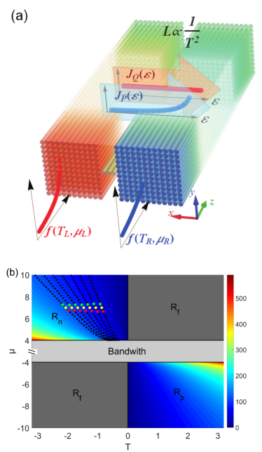
(a)

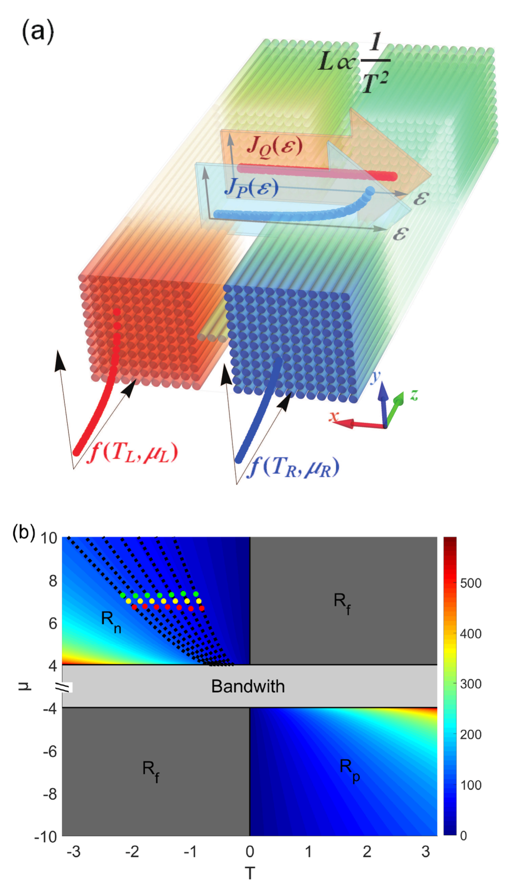
(b)

Figure 1: (a) Transport junction made from nonlinear waveguide arrays with square reservoirs. The two reservoirs are connected by one dimensional chain. The onsite energy of nodes is set to zero as the energy reference. Only nearest neighbor coupling $\kappa_{0}=1$ is considered. The system is initialized at lower end of the waveguides, and it relaxes toward equilibrium during propagating along $z$ direction, through heat and power transport across the junction in the $x$ direction. A generic violation of the Wiedemann-Franz law is predicted with the Lorentz number $L\propto T^{-2}$, indicating decoupled thermal ($J_{Q}$) and power ($J_{P}$) current [Eqs. (34-35)]. Shown in the inset is the energy dependence of $J_{Q}(\varepsilon)$ and $J_{P}(\varepsilon)$ for constant transmission $\mathcal{T}$. (b) $(T,\mu)$ phase diagram of the square reservoir. $R_{\rm p}$ and $R_{\rm n}$ represent the positive and negative temperature regime, respectively. No equilibrium state exists in the $R_{\rm f}$ regime. Power ($P$) for given $(T,\mu)$ is represented by the colored code. The black dashed lines are the iso-power lines. The red (green) dots are the initial parameters of the left (right) reservoir, while the yellow dots are their average $\bar{T}$ and $\bar{\mu}$.

Propagation of the optical modes along the waveguides is described by the discrete nonlinear Schrödinger equation (DNSE)[41, 42]

$$i\frac{d\psi_{m}}{dz}+\kappa\sum_{\{n\}}{\psi_{n}}+\chi\left|\psi_{m}\right|^{2}\psi_{m}=0,$$ (1)

with dimensionless parameters $\psi_{m}$, $\kappa$, $\chi$ representing the complex wave amplitude, the nearest neighbour coupling between waveguides and Kerr-type nonlinear coefficient, respectively. Here the coordinate $z$ along waveguide plays the role of time in standard Schrödinger equation, and $\{n\}$ includes all the nearest neighbours of $m$.

For weak nonlinear interactions, we can diagonalize the linear term and obtain the corresponding eigenmode (supermode) propagating constant $\beta_{k}$ and corresponding vector $\varphi_{k}$. For a given state $\psi$, the modal occupancy is obtained by projection onto each supermode $\left|c_{k}\right|^{2}=\left|\langle\varphi_{k}|\psi\rangle\right|^{2}$. The system evolves with conserved internal energy $U=\sum_{k=1}^{M}{\varepsilon_{k}\left|c_{k}\right|^{2}}$ and optical power $P=\sum_{k=1}^{M}{\left|c_{k}\right|^{2}}$, with the total number of modes $M$, the eigen energy defined by the negative of $\beta$ as $\varepsilon_{k}=-\beta_{k}$, and $\beta_{1}\geq\beta_{2}\geq\cdots\geq\beta_{M}$. The system thus has a bounded energy spectrum between $[\varepsilon_{1},\varepsilon_{M}]$. The weak nonlinear part introduces coupling among different supermodes, such that the system can thermalize to an equilibrium state through energy and power redistribution among supermodes. It plays a role similar to molecular collisions in the ideal gas model.

Equilibrium thermodynamic theory – We can use a recently developed optical thermodynamic theory to describe each reservoir[7]. The system internal energy can be written as (omitting the reservoir index)

$$U=MT+\mu P,$$ (2)

where $T$ is the dimensionless optical temperature, $\mu$ is the chemical potential. An optical entropy can be defined as

$$S=\sum_{k=1}^{M}{\ln\left|c_{k}\right|^{2}}.$$ (3)

Using the maximum entropy principle, at thermal equilibrium, the mode occupancy follows the classical Rayleigh-Jeans (R-J) distribution

$$f(\varepsilon_{k})=\left|c_{k}\right|^{2}=\frac{T}{\varepsilon_{k}-\mu}.$$ (4)

One prominent feature of the system is that, for given power $P$, the optical entropy $S$ no longer varies monotonically with the internal energy $U$ due to bounded energy spectrum. Consequently, the system can reach the negative optical temperature regime[7, 43]. From Eqs. (2-4), we have plotted the phase diagram of the reservoir with square lattice. As shown in Fig. 1b, only $\left\{\left(T,\mu\right)|T<0,\mu>\varepsilon_{M}\right\}$ and $\left\{\left(T,\mu\right)|T>0,\mu<\varepsilon_{1}\right\}$ can be visited, and the other regimes are forbidden($R_{f}$). This follows from the requirement $\left|c_{k}\right|^{2}\geq 0$. Moreover, the chemical potential is out of the band spectrum of the system, i.e., $\mu$ is below (above) the lowest (highest) energy of the spectrum for positive (negative) temperature. The positive and negative temperature regimes are anti-symmetric with each other in the phase diagram when neglecting the nonlinear effect. In the following, we focus on the negative temperature regime and numerically check that this anti-symmetry is still approximately valid in the weakly nonlinear regime (Fig. 3).

Transport coefficients in microcanonical ensemble – Transport theory is normally formulated with open boundaries using grand canonical ensemble. Due to the finite size of present junction, it is convenient to utilize the microcanonical setup. We extract the transport coefficients by following the thermalization process of a microcanonical system from given initial conditions. Using the theory of irreversible thermodynamics, we can obtain the evolution equations of $\Delta P$ and $\Delta T$ (See Appendix A). For symmetric junctions with identical left and right reservoirs, they read

$$\tau_{0}\frac{\partial}{\partial z}\left(\begin{array}[]{c}\Delta P\\ \Delta T\\ \end{array}\right)=-\left(\begin{matrix}1&-\kappa\alpha\\ -\frac{\alpha}{\ell\kappa}&\frac{L+\alpha^{2}}{\ell}\\ \end{matrix}\right)\left(\begin{array}[]{c}\Delta P\\ \Delta T\\ \end{array}\right)$$ (5)

where we have defined a transport timescale $\tau_{0}=\kappa/\left(2G\right)$ . Here, the reservoir properties $\kappa=\left.\left(\partial P/\partial\mu\right)\right|_{T}$, $\alpha_{r}=-\left.\left(\partial\mu/\partial T\right)\right|_{P}$, $C_{P}=\left.T\left(\partial S/\partial T\right)\right|_{P}$ are the compression coefficient, Seebeck coefficient and the heat capacity at constant power, respectively, with $l=C_{P}/T\kappa$. They can be obtained from the thermodynamic relations [Eqs. (15-17)]. The effective Seebeck coefficient $\alpha=\alpha_{r}-\alpha_{c}$ characterizes the difference between the reservoir itself $\alpha_{r}$ and the whole junction $\alpha_{c}$.

The general solution of the above equations are

$$\Delta P\left(z\right)=\left(\frac{\Omega+\delta-1}{2\Omega}\Delta P_{0}+\frac{\alpha\kappa}{2\Omega}\Delta T_{0}\right)e^{-\frac{z}{\tau_{>}}}\left[1+\frac{\left(\Omega-\delta+1\right)\Delta P_{0}-\alpha\kappa\Delta T_{0}}{\left(\Omega+\delta-1\right)\Delta P_{0}+\alpha\kappa\Delta T_{0}}e^{-\frac{z}{\tau_{<}}}\right],$$ (6)

$$\Delta T\left(z\right)=\left(\frac{\Omega-\delta+1}{2\Omega}\Delta T_{0}+\frac{\alpha}{2l\kappa\Omega}\Delta P_{0}\right)e^{-\frac{z}{\tau_{>}}}\left[1+\frac{l\kappa\left(\Omega+\delta-1\right)\Delta T_{0}-\alpha\Delta P_{0}}{l\kappa\left(\Omega-\delta+1\right)\Delta T_{0}+\alpha\Delta P_{0}}e^{-\frac{z}{\tau_{<}}}\right]$$ (7)

where $\delta=\left[1+\left(L+\alpha^{2}\right)/l\right]/2$ and $\varOmega=\sqrt{\delta^{2}-L/l}$ form the eigenvalues of the evolutionary matrix $\lambda_{\pm}=\delta\pm\varOmega$. The fast and slow timescales $\tau_{<}=\tau_{0}/2\varOmega$ and $\tau_{>}=\tau_{0}/\left(\delta-\varOmega\right)$ indicate the evolution of the system in two stages (Fig. 2): (1) A saturation process is characterized by the time scale $\tau_{<}$, which dominates the initial short time period. This process leads to an initial increase in the absolute value of the particle number deviation until it reaches a maximum . (2) A decay process is characterized by the time scale $\tau_{>}$, which dominates the longer period of time after saturation. The three transport coefficients $G$, $\alpha_{c}$ and $L$ (or $G_{T}$) can then be acquired by fitting the numerical results . Figure 2 shows results of fitting the transient evolution of the rectangular junction. The details can be found in Appendix A.2.

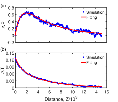
Figure 2: Evolution of (a) power ($\Delta P$) and (b) temperature ($\Delta T$) deviations from the average values $\bar{T}=-1.065$ and $\bar{\mu}=7$, with $\Delta T=0.13$, $\Delta\mu=-0.7$, $\chi=0.2$. The blue dots are numerical results, and the red line is fitting from Eqs. (6-7).

Numerical Results – Figure 3a-3d shows temperature dependence of the transport coefficients for a symmetric junction with square-lattice reservoirs. We notice that, in the negative temperature regime, conductance $G<0$, indicating that the power is transferred from the low to the high chemical potential reservoir when $\varDelta T=0$. This seemingly surprising result does not violate the second law of thermodynamics. Considering two subsystems that can exchange particles with each other under constant temperature, the second law of thermodynamics requires that the entropy does not decrease during the particle exchange

$$dS=\left(\frac{\mu_{L}}{T_{L}}-\frac{\mu_{R}}{T_{R}}\right)dP\geq 0$$ (8)

where $dP$ is the power lost from the left reservoir or gained from the right reservoir. When $T_{L}=T_{R}>0$, the power is transferred from high to low chemical potential. However, when $T_{L}=T_{R}<0$, the direction is reversed, meaning $G<0$. Since heat is transferred from high to low temperature in both positive and negative temperature regions, we have $G_{T}>0$.

Figure 3a shows an approximated linear $T$ dependence of $G$ for all the nonlinear parameters considered. This can be understood qualitatively from the Landauer formalism (Appendix B). The conductance can be approximated as

$$G=\int{\frac{d\varepsilon}{2\pi}{\mathcal{T}}(\varepsilon)\frac{T}{\left(\varepsilon-\mu\right)^{2}}},$$ (9)

indicating $G\propto T$ for temperature independent transmission $\mathcal{T}(\varepsilon)$. Moreover, the optical modes contribute to the transport with a weighting factor inversely proportional to the square of the energy deviation from the chemical potential.

(a)

(b)

(c)

(d)

Figure 3: Dependence of transport coefficients on temperature ($T$) for different nonlinear strengths $\chi$ at $\bar{\mu}=7$. (a) Conductance $G$, (b)Seebeck coefficient $\alpha_{c}$, (c) Thermal conductance $G_{T}$, (d) Lorenz number $L$. The inset shows dependence of $L$ on chemical potential $\mu$ at $T=-1.06$ and $\chi=0.2$. The black solid lines are theoretical results from the Landauer formalism. Results at positive temperature with $\chi=0.4$ are shown with empty squares. The sign of $T$ and $G$ at positive $T$ are reversed to show in the figure. They are very close to those at corresponding negative temperature (filled squares).

Temperature dependence of the Seebeck coefficient $\alpha_{c}$ is shown in Fig. 3b. It can be well fitted by an inverse $T$ dependence $\alpha_{c}\propto-1/T$ predicted by the Landauer model. The little effect of nonlinear interaction on $\alpha_{c}$ can also be captured by the Landuer result. In fact, $\alpha_{c}$ can be written as $\alpha_{c}=K_{1}/(K_{0}T)$. $K_{0}$ and $K_{1}$ have similar dependence on the nonlinear interaction, they cancel with each other in $\alpha_{c}$.

Similar to conductance, the thermal conductance $G_{T}$ also increases with nonlinearity (Fig. 3c). From the Landauer formalism, we get

$$G_{T}=\int{\frac{d\varepsilon}{2\pi}}\mathcal{T}(\varepsilon)-T\alpha_{c}^{2}G.$$ (10)

This gives a temperature independent $G_{T}$. Similar to $G$, the temperature dependence in the numerical results is due to nonlinear interaction. The second term on the right side of Eq. (10) represents correction to the thermal conductance due to Seebeck coefficient. Here, its magnitude is comparable to the first term. This is in contrast to the case of electrons in condensed matter system, where the thermoelectric correction is often negligible.

The variation of $L$ with temperature and chemical potential is shown in Fig. 3d, and is once again captured by Landauer’s theory. It can be found that the Lorenz number is more sensitive to temperature than the chemical potential (Inset). In the Landauer picture, $G_{T}\propto T^{0}$ together with $G\propto T$ leads to $L\propto 1/T^{2}$, which violates the W-F law. The decrease in $L$ with decreasing temperature comes from the increase in $\left|G\right|$. Similar to $\alpha_{c}$, we also observe a rather weak dependence on the strength of nonlinear interaction. Thus, the violation of W-F law here is not due to nonlinear interaction. Rather, its origin is similar to that in coherent mescoscopic conductors, which can be fully accounted by the single particle Landauer formalism.

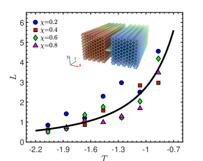
Figure 4: Variation of Lorenz number with temperature for different nonlinear strengths at $\bar{\mu}=7$ for a junction with hexagonal honeycomb reserviors (Inset). The black solid line is theoretical result from the Landauer formalism.

To further illustrate the violation of the W-F law, we considered a symmetric junction made from hexagonal honeycomb reservoirs with the same bandwidth (Fig. 1a). Junction with hexagonal reservoirs has a broader transmission spectrum compared to that with square reservoirs (Fig. B1a). This is due to the two van Hove singularities unique to hexagonal lattice, particularly evident in the DOS (Fig. B1b), giving higher transmission to the modes near the band edges. This makes the thermal conductivity increase to about twice that of the square case. As a result, we observe a more severe violation of the W-F law (Fig. 4), albeit with the same $1/T^{2}$ dependence.

Conclusions – We have developed a theory based on microcanonical ensemble to extract the transport coefficients of the coupled thermal and power transport in coupled waveguide arrays. We found a systematic violation of the Wiedemann-Franz law with the Lorenz number $L\propto 1/T^{2}$. The numerical results can be understood from the classical limit of Landauer formula. Our theory based on microcanonical ensemble is compatible to experimental realizations. Thus, it paves the way of studying fundamental nonequilibrium thermodynamic processes in parameters regimes that are unreachable in condensed matter and atomic gas systems.

This work was supported by the National Natural Science Foundation of China (Grant Nos. 22273029 and 21873033).

Appendix A Evolution equations for $\Delta P$ and $\Delta T$

Using the theory of irreversible thermodynamics, we can make connection between the driving affinities $\varDelta\mu$, $\varDelta T$ with the corresponding power ($I_{P}$) and entropy ($I_{S}$) fluxes, which follow the Onsager symmetry

$$\left(\begin{array}[]{c}I_{P}\\ I_{S}\\ \end{array}\right)=\left(\begin{matrix}K_{0}&K_{1}/T\\ K_{1}/T&K_{2}/T^{2}\\ \end{matrix}\right)\left(\begin{array}[]{c}\Delta\mu\\ \Delta T\\ \end{array}\right).$$ (11)

Positive direction of the current is chosen as from $L$ to $R$ reservoir. The matrix elements $K_{0}$, $K_{1}$ and $K_{2}$ depend on the state of the system and can be expressed in terms of the power conductance $G$, the thermal conductance $G_{T}$, the Seebeck coefficient $\alpha_{c}$ and the Lorenz number $L=G_{T}/TG$,

$$\frac{\partial}{\partial z}\left(\begin{array}[]{c}\Delta P\\ \Delta S\\ \end{array}\right)=-2G\left(\begin{matrix}1&\alpha_{{c}}\\ \alpha_{{c}}&L+\alpha_{{c}}^{2}\\ \end{matrix}\right)\left(\begin{array}[]{c}\Delta\mu\\ \Delta T\\ \end{array}\right)$$ (12)

Due to the weak link between the two reservoirs, bottleneck of the thermalization process is at the central chain. For the two reservoirs, the thermalization can be considered as a quasi-static process, where the two reservoirs can reach local equilibrium much faster than the whole junction. This can be verified by tracking the evolution of the system, and allows us to use the thermodynamic equation of the reservoirs. Using the Maxwell’s relations $\left.\left(\partial S/\partial\mu\right)\right|_{T}=\left.\left(\partial P/\partial T\right)\right|_{\mu}$ and $-\left.\left(\partial S/\partial P\right)\right|_{T}=\left.\left(\partial\mu/\partial T\right)\right|_{P}$, we can obtain

$$dP=\left.\frac{\partial P}{\partial\mu}\right|_{T}d\mu+\left.\frac{\partial P}{\partial T}\right|_{\mu}dT=\kappa d\mu+\alpha_{r}\kappa dT,$$ (13)

$$dS=\left.\frac{\partial S}{\partial P}\right|_{T}dP+\left.\frac{\partial S}{\partial T}\right|_{P}dT=\alpha_{r}dP+\kappa ldT$$ (14)

where $\kappa=\left.\left(\partial P/\partial\mu\right)\right|_{T}$, $\alpha_{r}=-\left.\left(\partial\mu/\partial T\right)\right|_{P}$, $l=C_{P}/T\kappa$ are the compression coefficient, Seebeck coefficient and Lorenz number of the reservoir, respectively, with $C_{P}=\left.T\left(\partial S/\partial T\right)\right|_{P}$ the reservoir heat capacity at constant power. In the linear response regime, they can be obtained from the equilibrium thermodynamic state at $\bar{T}$ and $\bar{\mu}$ as

$$\kappa=\left.\sum_{i}^{M}{\frac{T}{\left(\varepsilon_{i}-\mu\right)^{2}}}\right|_{T},$$ (15)

$$\alpha_{r}=\frac{1}{\kappa}\left.\sum_{i=1}^{M}{\frac{1}{\varepsilon_{i}-\mu}}\right|_{\mu},$$ (16)

$$C_{P}=M-T\alpha_{r}^{2}\kappa.$$ (17)

According to the thermodynamic equations, Eqs. (13-14), the optical power $P(z)$ and entropy $S(z)$ of the reservoir at position $z$ can be written as

$$P\left(z\right) =\kappa\mu\left(z\right)+\alpha_{r}\kappa T\left(z\right)+A,$$ (18)

$$S\left(z\right) =\alpha_{r}P\left(z\right)+\kappa lT\left(z\right)+B$$ (19)

where $A$ and $B$ are constants related to the initial conditions. We have dropped the reservoir index. When the left and right reservoirs are identical, their thermodynamic parameters are also identical, $A_{L}=A_{R}$ and $B_{L}=B_{R}$. Then, the optical power ($\Delta P\left(z\right)$) and entropy ($\Delta S\left(z\right)$) difference can be written as

$$\Delta P\left(z\right) =\kappa\Delta\mu\left(z\right)+\alpha_{r}\kappa\Delta T\left(z\right),$$ (20)

$$\Delta S\left(z\right) =\alpha_{r}\Delta P\left(z\right)+\kappa l\Delta T\left(z\right).$$ (21)

Using $\Delta P$ and $\Delta T$ to eliminate $\Delta S$ and $\Delta\mu$ in Eq. (12), the evolution equations are obtained

$$\tau_{0}\frac{\partial}{\partial z}\left(\begin{array}[]{c}\Delta P\\ \Delta T\\ \end{array}\right)=-\left(\begin{matrix}1&-\kappa\alpha\\ -\frac{\alpha}{\kappa l}&\frac{\alpha^{2}+L}{l}\\ \end{matrix}\right)\left(\begin{array}[]{c}\Delta P\\ \Delta T\\ \end{array}\right)\equiv-\varLambda\left(\begin{array}[]{c}\Delta P\\ \Delta T\\ \end{array}\right),$$ (22)

where we have defined a transport timescale $\tau_{0}=\kappa/\left(2G\right)$ and an effective Seebeck coefficient $\alpha=\alpha_{r}-\alpha_{c}$. The eigen values of matrix $\varLambda$ are

$$\lambda_{\pm}=\frac{1}{2}\left(1+\frac{\alpha^{2}+L}{l}\right)\pm\sqrt{\left(\frac{1}{2}+\frac{\alpha^{2}+L}{2l}\right)^{2}-\frac{L}{l}}=\delta\pm\varOmega.$$ (23)

General solutions of Eq. (22) can be expressed using the eigen values

$$\Delta P\left(z\right) =C_{1}e^{-\frac{\lambda_{+}}{\tau_{0}}z}+C_{2}e^{-\frac{\lambda_{-}}{\tau_{0}}z},$$ (24)

$$\Delta T\left(z\right) =C_{3}e^{-\frac{\lambda_{+}}{\tau_{0}}z}+C_{4}e^{-\frac{\lambda_{-}}{\tau_{0}}z},$$ (25)

where the coefficients $C_{1}$, $C_{2}$, $C_{3}$ and $C_{4}$ are determined by the initial conditions. Assuming that the initial power and temperature difference are $\Delta P_{0}$ and $\Delta T_{0}$, from Eqs. (22), (24) and (25) we get

$$C_{1} =\frac{1+\Omega-\delta}{2\Omega}\Delta P_{0}-\frac{\kappa\alpha}{2\Omega}\Delta T_{0},$$ (26)

$$C_{2} =\frac{\Omega+\delta-1}{2\Omega}\Delta P_{0}+\frac{\kappa\alpha}{2\Omega}\Delta T_{0},$$ (27)

$$C_{3} =-\frac{\alpha}{2\kappa l\Omega}\Delta P_{0}+\frac{\delta+\Omega-1}{2\Omega}\Delta T_{0},$$ (28)

$$C_{4} =\frac{\alpha}{2\kappa l\Omega}\Delta P_{0}+\frac{\Omega-\delta+1}{2\Omega}\Delta T_{0}.$$ (29)

Substituting into Eqs. (24) and (25), we can obtain the evolution equations for $\Delta P$ and $\Delta T$.

A.1 Numerical simulation

We choose the initial condition of each reservoir by fixing its optical temperature $T_{\alpha}$ and chemical potential $\mu_{\alpha}$. The corresponding optical power and internal energy can then be obtained. We perform calculations in the linear response regime with $T_{L}-T_{R}=\Delta T\ll\bar{T}$, $\mu_{L}-\mu_{R}=\Delta\mu\ll\bar{\mu}$. When the left and right reservoirs are identical, the average temperature and chemical potential are $\bar{T}=\left(T_{L}+T_{R}\right)/2$ and $\bar{\mu}=\left(\mu_{L}+\mu_{R}\right)/2$, respectively. Figure 1b shows seven sets of parameters at fixed chemical potential, all selected on iso-power lines while ensuring the small temperature and chemical potential difference. The fourth-order Runge-Kutta method was used to solve Eq. (1). The final result for each given initial condition is ensemble averaged by choosing different random phases for $c_{i}$. Fig. 2 shows the calculated results for a symmetric junction with square-lattice reservoirs at $\bar{T}=-1.065$ and $\bar{\mu}=7$. At the initial stage, driven by temperature and chemical potential deviations, the optical power is rapidly transferred from the cold reservoir to the hot reservoir. After $\Delta P$ reaches saturation, the system is brought to equilibrium by a slow relaxation process.

A.2 Data Fitting

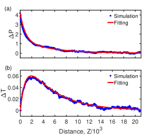
(a)

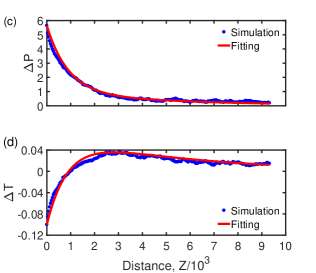
(b)

Figure A1: Evolution of power ($\varDelta P$) temperature ($\varDelta T$) difference as a function of propagating distance $z$ for two sets of parameters. (a-b) $\Delta P_{0}=4.1787$, $\Delta T_{0}=0$. (c-d) $\Delta P_{0}=5.6458$, $\Delta T_{0}=-0.1$. The fitting is performed using the same set of transport coefficients in (a-b) and (c-d).

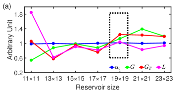
(a)

(b)

Figure A2: Convergence tests for two types of reservoirs with square (a) and hexagonal honeycomb (b) lattices. All transport coefficients are scaled to the same order of magnitude. The dashed boxes encloses reservoir size used in the main text.

We use Eqs. (6) and (7) to fit the evolution of $\varDelta P$ and $\varDelta T$ simultaneously by scanning the chain parameter space so that the residual $R$ is minimized, which is defined as[28]

$$R=\sum_{i}{\left[\left(\frac{\Delta P\left(z_{i}\right)-\Delta P_{i}}{\bar{P}}\right)^{2}+\left(\frac{\Delta T\left(z_{i}\right)-\Delta T_{i}}{\bar{T}}\right)^{2}\right]}.$$ (30)

Here, $\Delta P\left(z_{i}\right)$ and $\Delta T\left(z_{i}\right)$ are obtained from Eqs. (6) and (7) at position $z_{i}$, $\Delta P_{i}$ and $\Delta T_{i}$ are the numerically calculated results from Eq. (1) at $z_{i}$, and $\bar{P}$ and $\bar{T}$ are averages of $\Delta P_{i}$ and $\Delta T_{i}$. Since the calculation is in the linear response regime, our results are only related to the equilibrium temperature and chemical potential of the system, independent of the initial biases $\Delta P_{0}$ and $\Delta T_{0}$. This is checked in Fig. A1 where evolution from two sets of different initial conditions is fitted by the same set of transport coefficients.

A.3 Convergence tests

We performed convergence tests for symmetric junctions formed by square and hexagonal honeycomb lattices, respectively, to ensure that the fitted transport coefficients do not depend on the size of the reservoirs. The results are summarized in Fig. (A1). Parameters used in the main text are enclosed by dotted boxes.

Appendix B Landauer transport theory

The DNSE corresponds to an effective tight-binding Hamiltonian for the junction[7, 44]

$$H\left(\psi_{m},i\psi_{m}^{*}\right)=\sum_{\{m,n\}}{\kappa\psi_{m}^{*}\psi_{n}}+\frac{1}{2}\chi\sum_{m}{\left|\psi_{m}\right|^{4}}.$$ (31)

Here, $\psi_{m}$ and $i\psi_{m}^{*}$ form the canonical conjugate pairs, $\{m,n\}$ are nearest neighbour pairs. The first and the second term corresponds to the linear and nonlinear part of the Hamiltonian.

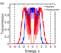
(a)

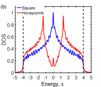
(b)

Figure B1: (a) The transmission spectrum of two symmetric junctions. The black dotted lines indicate the bandwidth of the systems. (b) The density of states of the two symmetric junctions.

We can also analyze the transport coefficients of the junction in the grand canonical ensemble using the Landauer formalism. For this purpose, we introduce two fictitious baths coupling to the boundary sites of the two reservoirs, respectively. The linear transport coefficients $G$, $\alpha_{c}$ and $G_{T}$ of the junction are given by the following integrals

$$K_{n}=\int_{\varepsilon_{\min}}^{\varepsilon_{\max}}{\frac{d\varepsilon}{2\pi}\left(\varepsilon-\mu\right)^{n}{\mathcal{T}}\left(\varepsilon\right)\left(-\frac{\partial f}{\partial\varepsilon}\right)}$$ (32)

where $f=T/\left(\varepsilon-\mu\right)$ is the R-J distribution function and ${\mathcal{T}}\left(\varepsilon\right)$ is the energy-dependent transmission coefficient, a central quantity in the Landauer formalism. It is given by the Caroli formula from the nonequilibrium Green’s function (NEGF) method as

$${\mathcal{T}}\left(\varepsilon\right)=\text{Tr}\left[G_{d}^{{\dagger}}\left(\varepsilon\right)\Gamma_{L}\left(\varepsilon\right)G_{d}\left(\varepsilon\right)\Gamma_{R}\left(\varepsilon\right)\right]$$ (33)

where $G_{d}=1/\left[\left(E+i\eta\right)I-H-\Sigma_{L}-\Sigma_{R}\right]$ and $G_{d}^{\dagger}$ are the retarded and advanced Green’s functions of the system, respectively. $\eta$ is a small positive quantity, $\Sigma_{\alpha}\left(\varepsilon\right)$ is the retarded self-energy due to coupling to bath $\alpha$, and $\Gamma_{\alpha}\left(\varepsilon\right)=-2\text{Im}\left[\Sigma_{\alpha}\left(\varepsilon\right)\right]$ is the corresponding broadening function. Under the wide band approximation, $\Sigma_{\alpha}$ can be regarded as an energy-independent constant, $\Sigma_{\alpha}=-i\gamma$, and $\gamma$ is a real parameter, which we choose as $\gamma=0.1$. The power and thermal current are written respectively as

$$J_{P} =\int_{0}^{+\infty}d\varepsilon\mathcal{T}(\varepsilon)(f_{L}(\varepsilon)-f_{R}(\varepsilon)),$$ (34)

$$J_{Q} =\int_{0}^{+\infty}d\varepsilon(\varepsilon-\mu)\mathcal{T}(\varepsilon)(f_{L}(\varepsilon)-f_{R}(\varepsilon)).$$ (35)

The density of states (DOS) of the system is obtained by $\rho\left(\varepsilon\right)=i\text{Tr}\left(G_{d}-G_{d}^{{\dagger}}\right)/M$. Figure B1 shows the transmission spectra and DOS of the two symmetric junctions, from which the transport coefficients of the systems can be calculated and analyzed.

References

- Yablonovitch [1987] E. Yablonovitch, Inhibited spontaneous emission in solid-state physics and electronics, Phys. Rev. Lett. 58, 2059 (1987).
- John [1987] S. John, Strong localization of photons in certain disordered dielectric superlattices, Phys. Rev. Lett. 58, 2486 (1987).
- Haldane and Raghu [2008] F. D. M. Haldane and S. Raghu, Possible realization of directional optical waveguides in photonic crystals with broken time-reversal symmetry, Phys. Rev. Lett. 100, 013904 (2008).
- Miri and Alù [2019] M.-A. Miri and A. Alù, Exceptional points in optics and photonics, Science 363, eaar7709 (2019).
- El-Ganainy et al. [2018] R. El-Ganainy, K. G. Makris, M. Khajavikhan, Z. H. Musslimani, S. Rotter, and D. N. Christodoulides, Non-hermitian physics and pt symmetry, Nat. Phys. 14, 11 (2018).
- Wright et al. [2022] L. G. Wright, F. O. Wu, D. N. Christodoulides, and F. W. Wise, Physics of highly multimode nonlinear optical systems, Nat. Phys. 18, 1018 (2022).
- Wu et al. [2019] F. O. Wu, A. U. Hassan, and D. N. Christodoulides, Thermodynamic theory of highly multimoded nonlinear optical systems, Nat. Photonics 13, 776 (2019).
- Parto et al. [2019] M. Parto, F. O. Wu, P. S. Jung, K. Makris, and D. N. Christodoulides, Thermodynamic conditions governing the optical temperature and chemical potential in nonlinear highly multimoded photonic systems, Opt. Lett. 44, 3936 (2019).
- Makris et al. [2020] K. G. Makris, F. O. Wu, P. S. Jung, and D. N. Christodoulides, Statistical mechanics of weakly nonlinear optical multimode gases, Opt. Lett. 45, 1651 (2020).
- Krupa et al. [2017] K. Krupa, A. Tonello, B. M. Shalaby, M. Fabert, A. Barthélémy, G. Millot, S. Wabnitz, and V. Couderc, Spatial beam self-cleaning in multimode fibres, Nat. Photonics 11, 237 (2017).
- Liu et al. [2016] Z. Liu, L. G. Wright, D. N. Christodoulides, and F. W. Wise, Kerr self-cleaning of femtosecond-pulsed beams in graded-index multimode fiber, Opt. Lett. 41, 3675 (2016).
- Niang et al. [2019] A. Niang, T. Mansuryan, K. Krupa, A. Tonello, M. Fabert, P. Leproux, D. Modotto, O. N. Egorova, A. E. Levchenko, D. S. Lipatov, S. L. Semjonov, G. Millot, V. Couderc, and S. Wabnitz, Spatial beam self-cleaning and supercontinuum generation with Yb-doped multimode graded-index fiber taper based on accelerating self-imaging and dissipative landscape, Opt. Express 27, 24018 (2019).
- Herr et al. [2014] T. Herr, V. Brasch, J. D. Jost, C. Y. Wang, N. M. Kondratiev, M. L. Gorodetsky, and T. J. Kippenberg, Temporal solitons in optical microresonators, Nat. Photonics 8, 145 (2014).
- Wright et al. [2015] L. G. Wright, D. N. Christodoulides, and F. W. Wise, Controllable spatiotemporal nonlinear effects in multimode fibres, Nat. Photonics 9, 306 (2015).
- Kalashnikov and Wabnitz [2022] V. L. Kalashnikov and S. Wabnitz, Stabilization of spatiotemporal dissipative solitons in multimode fiber lasers by external phase modulation, Laser Phys. Lett. 19, 105101 (2022).
- Wright et al. [2017] L. G. Wright, D. N. Christodoulides, and F. W. Wise, Spatiotemporal mode-locking in multimode fiber lasers, Science 358, 94 (2017).
- Jung et al. [2022] P. S. Jung, G. G. Pyrialakos, F. O. Wu, M. Parto, M. Khajavikhan, W. Krolikowski, and D. N. Christodoulides, Thermal control of the topological edge flow in nonlinear photonic lattices, Nat. Commun. 13, 4393 (2022).
- Pyrialakos et al. [2022] G. G. Pyrialakos, H. Ren, P. S. Jung, M. Khajavikhan, and D. N. Christodoulides, Thermalization Dynamics of Nonlinear Non-Hermitian Optical Lattices, Phys. Rev. Lett. 128, 213901 (2022).
- Shi et al. [2021] C. Shi, T. Kottos, and B. Shapiro, Controlling optical beam thermalization via band-gap engineering, Phys. Rev. Res. 3, 033219 (2021).
- Leykam et al. [2021] D. Leykam, E. Smolina, A. Maluckov, S. Flach, and D. A. Smirnova, Probing Band Topology Using Modulational Instability, Phys. Rev. Lett. 126, 073901 (2021).
- Bloch et al. [2022] J. Bloch, I. Carusotto, and M. Wouters, Non-equilibrium Bose–Einstein condensation in photonic systems, Nat. Rev. Phys. 4, 470 (2022).
- Xiong et al. [2022] Z. Xiong, F. O. Wu, J.-T. Lü, Z. Ruan, D. N. Christodoulides, and Y. Chen, -space thermodynamic funneling of light via heat exchange, Phys. Rev. A 105, 033529 (2022).
- Baudin et al. [2020] K. Baudin, A. Fusaro, K. Krupa, J. Garnier, S. Rica, G. Millot, and A. Picozzi, Classical Rayleigh-Jeans Condensation of Light Waves: Observation and Thermodynamic Characterization, Phys. Rev. Lett. 125, 244101 (2020).
- Callen and Welton [1951] H. B. Callen and T. A. Welton, Irreversibility and generalized noise, Phys. Rev. 83, 34 (1951).
- Brantut et al. [2013] J.-P. Brantut, C. Grenier, J. Meineke, D. Stadler, S. Krinner, C. Kollath, T. Esslinger, and A. Georges, A Thermoelectric Heat Engine with Ultracold Atoms, Science 342, 713 (2013).
- Nietner et al. [2014] C. Nietner, G. Schaller, and T. Brandes, Transport with ultracold atoms at constant density, Phys. Rev. A 89, 013605 (2014).
- Gallego-Marcos et al. [2014] F. Gallego-Marcos, G. Platero, C. Nietner, G. Schaller, and T. Brandes, Nonequilibrium relaxation transport of ultracold atoms, Phys. Rev. A 90, 033614 (2014).
- Häusler et al. [2021] S. Häusler, P. Fabritius, J. Mohan, M. Lebrat, L. Corman, and T. Esslinger, Interaction-Assisted Reversal of Thermopower with Ultracold Atoms, Phys. Rev. X 11, 021034 (2021).
- [29] E. L. Hazlett, L.-C. Ha, and C. Chin, Anomalous thermoelectric transport in two-dimensional Bose gas, arXiv:1306.4018 .
- Papoular et al. [2014] D. J. Papoular, L. P. Pitaevskii, and S. Stringari, Fast thermalization and helmholtz oscillations of an ultracold bose gas, Phys. Rev. Lett. 113, 170601 (2014).
- Rançon et al. [2014] A. Rançon, C. Chin, and K. Levin, Bosonic thermoelectric transport and breakdown of universality, New J. Phys. 16, 113072 (2014).
- Uchino and Brantut [2020] S. Uchino and J.-P. Brantut, Bosonic superfluid transport in a quantum point contact, Phys. Rev. Research 2, 023284 (2020).
- Husmann et al. [2015] D. Husmann, S. Uchino, S. Krinner, M. Lebrat, T. Giamarchi, T. Esslinger, and J.-P. Brantut, Connecting strongly correlated superfluids by a quantum point contact, Science 350, 1498 (2015).
- Husmann et al. [2018] D. Husmann, M. Lebrat, S. Häusler, J.-P. Brantut, L. Corman, and T. Esslinger, Breakdown of the wiedemann–franz law in a unitary Fermi gas, Proc. Natl. Acad. Sci. U.S.A. 115, 8563 (2018).
- Lee et al. [2017] S. Lee, K. Hippalgaonkar, F. Yang, J. Hong, C. Ko, J. Suh, K. Liu, K. Wang, J. J. Urban, X. Zhang, C. Dames, S. A. Hartnoll, O. Delaire, and J. Wu, Anomalously low electronic thermal conductivity in metallic vanadium dioxide, Science 355, 371 (2017).
- Note [1] It plays the role of particle number here. Thus, power conservation corresponds to particle number conservation.
- Baldovin et al. [2021] M. Baldovin, S. Iubini, R. Livi, and A. Vulpiani, Statistical mechanics of systems with negative temperature, Phys. Rep. 923, 1 (2021).
- Marques Muniz et al. [2023] A. Marques Muniz, F. Wu, P. Jung, M. Khajavikhan, D. Christodoulides, and U. Peschel, Observation of photon-photon thermodynamic processes under negative optical temperature conditions, Science 379, 1019 (2023).
- Agraït et al. [2003] N. Agraït, A. L. Yeyati, and J. M. van Ruitenbeek, Quantum properties of atomic-sized conductors, Phys. Rep. 377, 81 (2003).
- Krinner et al. [2017] S. Krinner, T. Esslinger, and J.-P. Brantut, Two-terminal transport measurements with cold atoms, J. Phys. Condens. Matter 29, 343003 (2017).
- Lederer et al. [2008] F. Lederer, G. I. Stegeman, D. N. Christodoulides, G. Assanto, M. Segev, and Y. Silberberg, Discrete solitons in optics, Phys. Rep. 463, 1 (2008).
- Agrawal [2001] G. Agrawal, Applications of Nonlinear Fiber Optics, Optics and photonics (Elsevier Science, 2001).
- Wu et al. [2020] F. O. Wu, P. S. Jung, M. Parto, M. Khajavikhan, and D. N. Christodoulides, Entropic thermodynamics of nonlinear photonic chain networks, Commun. Phys. 3, 216 (2020).
- Rasmussen et al. [2000] K. Ø. Rasmussen, T. Cretegny, P. G. Kevrekidis, and N. Grønbech-Jensen, Statistical Mechanics of a Discrete Nonlinear System, Phys. Rev. Lett. 84, 3740 (2000).