Rotating detectors in dS/AdS

Abstract

We analyse several aspects of detectors with uniform acceleration $a$ and uniform rotation $\Omega$ in de Sitter ($\Lambda>0$) and anti-de Sitter ($\Lambda<0$) spacetimes, focusing particularly on the periodicity, in (Euclidean) proper time $\tau_{\rm traj}$, of geodesic interval $\tau_{\rm geod}$ between two events on the trajectory. For $\Lambda<0$, $\tau_{\rm geod}$ is periodic in ${\rm i}\tau_{\rm traj}$ for specific values of $a$ and $\Omega$. These results are used to obtain numerical plots for the response rate $\dot{\mathcal{F}}$ of Unruh-de Witt detectors, which display non-trivial combined effects of rotation and curvature through the dimensionless parameter $\Lambda c^{2}/\Omega^{2}$. In particular, periodicity does not imply thermality due to additional poles in the Wightman function away from the imaginary axis. We then present some results for stationary rotational motion in arbitrary curved spacetime, as a perturbative expansion in curvature.

I Introduction

Studying physical processes in a uniformly accelerated frame of reference in Minkowski spacetimeFulling (1973); Davies (1975); Unruh (1976) often forms a first step towards understanding these processes in curved spacetime. The mapping between these is provided by the so called principle of equivalence. However, by its very nature, the equivalence principle gives no insights into the quantitative role of curvature in these processes. One can obtain curvature corrections perturbatively, of course, but such results are of limited interest from a conceptual point of view since the limit of zero acceleration can not then be taken. A well known resultDeser and Levin (1997, 1998, 1999) that illustrates this is the response of a uniformly accelerated Unruh-de Witt detector in de Sitter spacetime with cosmological constant $\Lambda$, which is thermal with a temperature proportional to $\sqrt{a^{2}+\Lambda}$. A perturbative analysis would yield the leading curvature correction at $O(\Lambda/a^{2})$, and miss the $a\to 0$ limit.

In a recent work Hari and Kothawala (2021), it was shown that similar contribution due to (electric part of) Riemann tensor arises in general curved spacetimes, of which the (anti-) de Sitter results are but special cases. A remarkable partial summation of an infinite series once again yields new insights that one could not have gained from a naive application of the equivalence principle.

In this paper, we broaden the scope of such results by considering uniformly accelerating and rotating detectors in maximally symmetric spacetimes and obtaining certain exact results that should be relevant for the response of such detectors. We also give the result for arbitrary curved spacetimes, but, unfortunately, we are forced to leave it as a perturbation expansion since we have not been able to re-sum even a subset of terms in presence of rotation. Nevertheless, the exact results we present for rotating detectors in dS/AdS spacetimes by themselves yield important insights into the non-trivial of $\Lambda$ (including its sign) on the response of the detectors.

Three key results derived in this work are:

1. Relation between proper time and geodesic interval: Remarkably, the relation between the geodesic distance, $\Delta\tau_{\rm geod}$ and proper time distance, $\Delta\tau_{\rm traj}$ for a stationary trajectory with constant acceleration and constant torsion in a maximally symmetric spacetime can be expressed in a form closely resembling the structure in Minkowski spacetime (see Eqs. (14)

2. Periodicity in $\Delta\tau_{\rm geod}^{2}$: The above result yields the condition for periodicity of $\Delta\tau_{\rm geod}^{2}$ in Euclidean proper time ($\Delta\tau_{\rm traj}\rightarrow i\Delta t_{\rm traj}$) for $\Lambda<0$, for specific values of acceleration and torsion.

3. General spacetime: We also obtain a perturbative expression for $\Delta\tau_{\rm geod}^{2}$ for stationary trajectories in arbitrary curved spacetime, assuming derivatives of Riemann to be small.

The (square of) geodesic interval, $\sigma(x,x^{\prime})^{2}=-\Delta\tau_{\text{geod}}^{2}(x,x\prime)$ between two points on a trajectory is an important quantity that appears prominently in the analysis of classical as well quantum measurement processes in curved spacetimes. The latter, for instance, through its appearance in the leading short distance (Hadamard) form of the two point function

$$G_{\rm H}(x,y)=\frac{{\Delta^{1/2}(x,y)}}{\sigma(x,y)^{2}}+\ldots$$ (1)

where $\Delta(x,y)$ is the van Vleck determinant, derived again from $\sigma^{2}$. Amongst many things, the above form serves as the key mathematical tool to evaluate the response of an Unruh-deWitt detector coupled to quantum field in an arbitrary curved spacetime.

II Stationary motion

The trajectory of a timelike curve is specified using functions $x^{a}(\tau)$ defined at each point of the curve, with $\tau$ as the proper time along the curve. A more elegant way to represent the trajectory is through its curvature invariants, which, in four dimensions, are acceleration, torsion, and hypertorsion. At every point on the trajectory an orthonormal tetrad, $e^{\textsf{i}}_{a}$ can be constructed from the derivatives of $x^{a}(\tau)$, which satisfy the condition,

$$e^{\textsf{i}}_{a}e_{\textsf{i}b}=\eta_{ab}$$ (2)

Here, $\eta_{ab}=\text{diag}(-1,1,1,1)$. These tetrads serve as the basis vectors for the vector space at each point on the worldline. They obey the Serret-Frenet equations given by,

$$\frac{De^{\textsf{i}}_{a}}{\mathrm{d}\tau}=K_{a}^{\phantom{a}b}e^{\textsf{i}}_{b}$$ (3)

where the structure of the matrix $K_{ab}$ is given by,

$$K_{ab}=\begin{bmatrix}0&-a(\tau)&0&0\\ a(\tau)&0&\Omega(\tau)&0\\ 0&-\Omega(\tau)&0&\lambda(\tau)\\ 0&0&-\lambda(\tau)&0\\ \end{bmatrix}$$ (4)

where $a(\tau)$ is the magnitude of acceleration, $\Omega(\tau)$ is the torsion, and $\lambda(\tau)$ is the hypertorsion. These are the curvature invariants of the trajectory. Note that the matrix $K_{ab}$ is antisymmetric, $K_{ab}=-K_{ba}$. The worldline is stationary when these invariants are constant and do not depend on the parameter $\tau$. These stationary worldlines are classified into six categories (see Ref. Letaw (1981); Letaw and Pfautsch (1982, 1981)) for Minkowski spacetime according to the values of curvature invariants.

For a stationary trajectory, let $u^{i}(\tau)$ be the 4-velocity and $n^{i}(\tau)$ be the unit vector along the direction of 4-acceleration. We will be using Serret-Frenet equations to construct the tetrads and will express the worldline in terms of the tetrads at $\tau=0$. One starts with the tangent vector to the curve, and a unit vector in the direction of acceleration, from which remaining orthogonal vectors are obtained using Gram-Schmidt orthogonalization.

$$\nabla_{\bf u}u^{k} = a\,n^{k}\;;\quad\nabla_{\bf u}n^{k}=\Omega\,b^{k}+a\,u^{k}\;;$$

$$\quad\nabla_{\bf u}b^{k} = \lambda\,d^{k}-\Omega\,n^{k}\;;\quad\nabla_{\bf u}d^{k}=-\lambda\,b^{k}$$ (5)

Here, $\nabla_{\bf u}$ is the covariant derivative, $n^{k}=a^{k}/a$ is the normal vector in the direction of acceleration, $b^{k}$ is the binormal orthogonal to $u^{k}$ and $a^{k}$, and $d^{k}$ is another unit vector orthogonal to all other unit vectors. These equations are more succinctly expressed in terms of the Fermi derivative defined by,

$$\frac{D_{F}Y^{i}}{\mathrm{d}\tau}=\nabla_{\bf u}Y^{i}+\Omega^{i}_{\phantom{i}k}Y^{k}=0$$

where, $\Omega^{ik}:=a^{i}u^{k}-u^{i}a^{k}+\omega^{ik}$ and $\omega^{ik}:=\varepsilon^{ikjl}u_{j}\omega_{l}$. For stationary motion, $K_{ab}=\Omega_{ba}$.

The key geometrical quantity, which will also be our main focus, is the geodesic distance between two points on a stationary trajectory characterized by Serret-Frenet equations. To do this, we will follow the method sketched in Hari and Kothawala (2021). This method essentially uses Riemann normal coordinates (RNC) to solve for the trajectory as a power series

$$x^{i}(\tau)=\sum_{n=0}^{\infty}\frac{\tau^{n}}{n!}\left[\frac{\mathrm{d}^{n}x^{i}}{\mathrm{d}\tau^{n}}\right]_{\tau=0}$$ (6)

in which the coefficients on the RHS are determined by taking higher derivatives of the defining equation

$$\frac{\mathrm{d}^{2}x^{i}}{\mathrm{d}\tau^{2}}+\Gamma^{i}_{bc}\frac{\mathrm{d}x^{b}}{\mathrm{d}\tau}\frac{\mathrm{d}x^{c}}{\mathrm{d}\tau}=a^{i}$$ (7)

and using the Serret-Frenet equations. This method was explained and used in Hari and Kothawala (2021) for rectilinear, uniformly accelerated motion in arbitrary curved spacetime, and was shown to yield a remarkable result involving an analytically resummable piece of an otherwise infinite (perturbative) expansion. In this work, we will explore the effects of rotation to see if a similar result holds in this case.

III Maximally symmetric spacetimes

As a first step towards studying stationary trajectories in arbitrary curved spacetime, we will consider stationary trajectories in maximally symmetric spacetimes. As we will show, some very interesting analytic results can be obtained in this case, with several remarkable similarities and mappings with the corresponding results in Minkowski spacetime, which we have discussed in Appendix A; we will refer to the results in this appendix after deriving the corresponding results in maximally symmetry.

We will mostly use the metric of maximally symmetric spacetimes in embedding coordinates $X^{i}$, given byWeinberg (1972),

$$g_{ab}=\eta_{ab}+\frac{\Lambda}{1-\Lambda\eta_{ij}X^{i}X^{j}}\eta_{ac}\eta_{bd}X^{c}X^{d}$$ (8)

Then the Christoffel connections can be expressed as $\Gamma^{a}_{bc}=\Lambda X^{a}g_{bc}$. It can be easily shown that the stationary motion with acceleration and torsion will be always in the hyperplane $u^{i}(0)$-$n^{i}(0)$-$b^{i}(0)$ using Serret-Frenet equations.

III.1 Trajectory and geodesic distance

Further, using Eq. (5) and Eq. (7) the Taylor series expansion for the trajectory similar to Minkowski spacetime can be obtained as,

$$\frac{\mathrm{d}X^{i}}{\mathrm{d}\tau} = U^{i}$$

$$\frac{\mathrm{d}^{2}X^{i}}{\mathrm{d}\tau^{2}} = aN^{i}+\Lambda X^{i}$$

$$\frac{\mathrm{d}^{3}X^{i}}{\mathrm{d}\tau^{3}} = a\,\Omega\,B^{i}+a^{2}\frac{\mathrm{d}X^{i}}{\mathrm{d}\tau}$$

$$\frac{\mathrm{d}^{\mathsf{p}}X^{i}}{\mathrm{d}\tau^{\mathsf{p}}} = (a^{2}-\Omega^{2}+\Lambda)\frac{\mathrm{d}^{\mathsf{p}-2}X^{i}}{\mathrm{d}\tau^{\mathsf{p}-2}}+\Omega^{2}\Lambda\frac{\mathrm{d}^{\mathsf{p}-4}X^{i}}{\mathrm{d}\tau^{\mathsf{p}-2}}$$

Here, $\mathsf{p}\geq 4$, $U^{i}$, $N^{i}$, $B^{i}$ are similar to unit vectors $u^{i}$, $n^{i}$, $b^{i}$ in Minkowski spacetime, but now defined using the embedding coordinates. The above equations are obtained by expanding the covariant derivatives and using the Christoffel connections previously described. Solving the recursion equation will determine all the higher-order terms. The terms in each direction can be summed into hyperbolic functions, $\sinh$ and $\cosh$. The final form of the summed series expressing the trajectory is,

$$Z^{i}(\tau) = a\left[\cosh\left(q_{+}\tau\right)-\cosh\left(q_{-}\tau\right)\right]\,N^{i}(0)-\frac{a\,\Omega}{q_{+}q_{-}q_{0}}\left[q_{+}\sinh\left(q_{-}\tau\right)-q_{-}\sinh\left(q_{+}\tau\right)\right]\,B^{i}(0)$$ (9)

$$+\frac{1}{q_{+}q_{-}q_{0}^{2}}\left[(q_{-}^{2}+\Omega^{2})q_{+}\sinh\left(q_{-}\tau\right)-(q_{+}^{2}+\Omega^{2})q_{-}\sinh\left(q_{+}\tau\right)\right]\,U^{i}(0)$$

Here, $q_{0}:=\left[(a^{2}-\Omega^{2}+\Lambda)^{2}+4\Lambda\Omega^{2}\right]^{1/4}$ and $q_{\pm}:=(1/\sqrt{2})\sqrt{(a^{2}-\Omega^{2}+\Lambda)\pm q_{0}^{2}}$. These constants are similar to the ones obtained for stationary motion with all curvature invariants. In fact, there seems to be mapping between these trajectories, which will be discussed soon.

The mapping between the embedding coordinates and the RNC is given byHari and Kothawala (2020),

$$X^{i}=\Delta^{-1/(D-1)}\hat{x}^{i}$$ (10)

where, $\Delta=\Delta(0,\hat{x})$ is the van Vleck determinant with $D$ as the dimension of spacetime. The geodesic distance can be evaluated using the expression for flat spacetime, $-\Delta\tau_{\rm geod}=\eta_{ab}\hat{x}^{a}\hat{x}^{b}=\eta_{ab}Z^{a}Z^{b}\Delta^{2/(D-1)}$. For maximally symmetric spacetimes, we can use the formula, $\Delta^{2/(D-1)}=\Lambda\Delta\tau_{\rm geod}^{2}/\sin^{2}(-\Delta\tau_{\rm geod}\sqrt{\Lambda})$ for van Vleck determinant and simplify the equation for geodesic distance to obtain,

$$\Delta\tau_{\rm geod}^{2}=-\frac{1}{\Lambda}\left[\sin^{-1}\left(\sqrt{-\Lambda\Delta\tau_{\rm ms}^{2}}\right)\right]^{2}$$ (11)

Here, $\Delta\tau_{\rm ms}^{2}:=-(\eta_{ab}Z^{a}Z^{b})$ given by,

$$\Delta\tau_{\rm ms}^{2} = \Delta\widetilde{\tau}^{2}\left(1+\frac{1}{4}\Lambda\Delta\widetilde{\tau}^{2}\right)$$ (12)

$$\Delta\widetilde{\tau}^{2} = \frac{4}{q_{0}^{2}}\left[\left(1+\frac{\Omega^{2}}{q_{+}^{2}}\right)\sinh^{2}\left(\frac{q_{+}\Delta\tau_{\rm traj}}{2}\right)-\left(1+\frac{\Omega^{2}}{q_{-}^{2}}\right)\sinh^{2}\left(\frac{q_{-}\Delta\tau_{\rm traj}}{2}\right)\right]$$ (13)

Equation 11 can be rearranged using Eq. (12) to a similar form as obtained in Eq. (23) of Hari and Kothawala (2021),

$$\Delta\tau_{\rm geod}^{2}=\frac{4}{\Lambda}\left[\sinh^{-1}\left(\frac{1}{2}\sqrt{\Lambda\Delta\widetilde{\tau}^{2}}\right)\right]^{2}$$ (14)

The equation for the hyperbolic trajectory in the ref. Hari and Kothawala (2021) will be a special case when $\Omega=0$.

III.2 Periodicity in $\Delta\tau_{\rm geod}^{2}$

The periodicity in $\Delta\tau_{\rm geod}^{2}$ for Euclidean time($\Delta\tau_{\rm traj}\rightarrow i\Delta t_{\rm traj}$) can be analysed using Eq. (13). Equation 13 will be periodic only when both conditions given below are satisfied.

i) $\{q_{+},q_{-}\}\in\mathbb{R}$

ii) $q_{+}/q_{-}\in\mathbb{Q}$

The first condition restricts $q_{-}\in\mathbb{R}$, which implies

$$1-\sqrt{1+\frac{4\Lambda\Omega^{2}}{a^{2}-\Omega^{2}+\Lambda}}>0,\quad\sqrt{a^{2}-\Omega^{2}+\Lambda}>0$$

The above inequalities are only satisfied for $\Lambda<0$ and $a^{2}>\Omega^{2}+|\Lambda|$.

Using the first condition, the second condition can be simplified as,

$$\frac{q_{+}}{q_{-}}=\frac{\sqrt{1+\sqrt{1-\frac{4|\Lambda|\Omega^{2}}{(a^{2}-\Omega^{2}-|\Lambda|)^{2}}}}}{\sqrt{1-\sqrt{1-\frac{4|\Lambda|\Omega^{2}}{(a^{2}-\Omega^{2}-|\Lambda|)^{2}}}}}=r$$

$$\implies\frac{|\Lambda|\Omega^{2}}{(a^{2}-\Omega^{2}-|\Lambda|)^{2}}=\frac{r^{2}}{(r^{2}+1)^{2}}$$ (15)

Here, $r\in\mathbb{Q}$ and $r>1$. The above condition ensures that $q_{+}$ and $q_{-}$ are commensurable. Therefore, the conditions for periodicity in $\Delta\tau_{\rm geod}^{2}$ can be summarized as:

$$\Lambda < 0$$

$$a^{2} > \Omega^{2}+|\Lambda|$$

$$\frac{|\Lambda|\Omega^{2}}{(a^{2}-\Omega^{2}-|\Lambda|)^{2}} = \frac{r^{2}}{(r^{2}+1)^{2}}$$

III.3 Mappings between stationary motions in Minkowski and dS/AdS.

1. Helical motion in Minkowski and rotation in dS/AdS:

The RHS of Eq. (13) and Eq. (32) have a striking similarity. The functional form of these equations are similar. If we try compare the constants, the mapping between these equations can be summarized as,

Minkowski	Maximally symmetric
$a_{\eta}^{2}$	$a^{2}+\Lambda$
$\Omega_{\eta}^{2}$	$a^{2}(\Omega^{2}/(a^{2}+\Lambda))$
$\lambda^{2}$	$\Lambda(\Omega^{2}/(a^{2}+\Lambda))$

Note that $\Omega_{\eta}^{2}+\lambda^{2}=\Omega^{2}$. The curvature constant of maximally symmetric spacetime, $\Lambda$, plays a similar role of hypertorsion, $\lambda$ in flat spacetime.

2. Rotation in Minkowski and rotation in dS/AdS with $a=\Omega$:

In the case of maximally symmetric spacetimes, when the acceleration and torsion are equal, Eq. (12) reduces to,

$$\Delta\tau_{\rm ms}^{2}=\frac{4(\Lambda+\Omega^{2})}{\Lambda^{2}}\sinh^{2}\left(\frac{\sqrt{\Lambda}}{2}\Delta\tau_{\rm traj}\right)-\frac{\Omega^{2}\Delta\tau_{\rm traj}^{2}}{\Lambda}$$ (16)

The mapping between the flat spacetime and maximally symmetric spacetime for this motion is, $a_{\eta}^{2}\rightarrow a^{2}+\Lambda$ and $\Omega_{\eta}\rightarrow a=\Omega$.

IV General Spacetime

We now turn focus on arbitrary curved spacetimes, hoping again to obtain the relation between the geodesic interval and the proper time interval for points on stationary trajectories in these spacetimes, characterised again through Serret-Ferret conditions. The method we will employ is the one based on a judicious use of RNC, described in Sec. II of Ref. Hari and Kothawala (2021). The RNC is setup at some initial point $p_{0}$ and the trajectory of the probe at the point $p$ is expressed using Eq. (6). From the definitions of RNC we have, $\hat{z}^{a}(\Delta\tau)=\hat{x}^{a}(p)=\left(\Delta\tau_{\text{geod}}\right)\hat{t}^{a}(0;\Delta\tau)$ and $(\Delta\tau_{\text{geod}})^{2}=\eta_{ab}{\widehat{z}}^{a}(\Delta\tau){\widehat{z}}^{b}(\Delta\tau)$, where $\hat{t}^{a}$ is the tangent vector along the geodesic curve connecting the points $p_{0}$ and $p$. Utilizing Eq. (7) and its higher derivatives in RNC along with Serret-Frenet equations, each terms in the series can be obtained as,

$$\dot{\widehat{z}^{i}}(0) = u^{i}\rvert_{p_{0}}=u^{i}(0)$$

$$\ddot{\widehat{z}^{i}}(0) = \left[a\,n^{i}-\Gamma^{i}_{mk}u^{m}u^{k}\right]_{p_{0}}=\left[a\,n^{i}\right]_{p_{0}}$$

$$\dddot{\widehat{z}^{i}}(0) = \left[a\,u^{k}{\partial}_{k}n^{i}-\Gamma^{i}_{mj,k}u^{k}u^{m}u^{j}-2\Gamma^{i}_{mj}(u^{k}{\partial}_{k}u^{j})\right]_{p_{0}}$$

$$= \left[a\,\nabla_{\bm{u}}n^{i}-3\Gamma^{i}_{km}u^{k}a^{m}-\Gamma^{i}_{mj,k}u^{k}u^{m}u^{j}\right.$$

$$\left.+\Gamma^{i}_{mj}\Gamma^{j}_{kl}u^{m}u^{k}u^{l}\right]_{p_{0}}$$

$$= \left[a\,\nabla_{\bm{u}}n^{i}-\Gamma^{i}_{mj,k}u^{k}u^{m}u^{j}\right]_{p_{0}}$$

$$= \left[a\,\Omega\,b^{i}+a^{2}\,u^{i}-\Gamma^{i}_{mj,k}u^{k}u^{m}u^{j}\right]_{p_{0}}$$

The Christoffel connections in the above terms are evaluated using the series expansions in RNC. In the case of non-rotating motion ($\Omega=0$), this procedure gave the following series in Ref. Hari and Kothawala (2021),

$$\Delta\tau_{\rm geod}^{2} =\tau^{2}_{\rm acc}+\frac{1}{12}a^{2}{\tau}^{4}_{\rm acc}+\frac{1}{360}\left(a^{4}+3a^{2}{\mathscr{E}}_{n}\right){\tau}^{6}_{\rm acc}$$

$$\quad+\frac{1}{20160}\left(a^{6}+17a^{2}{\mathscr{E}}_{n}^{2}+18a^{4}{\mathscr{E}}_{n}\right){\tau}^{8}_{\rm acc}$$

$$\quad+\frac{1}{1814400}\left(a^{8}+81a^{6}{\mathscr{E}}_{n}+339a^{4}{\mathscr{E}}_{n}^{2}\right.$$

$$\left.\quad+155a^{2}{\mathscr{E}}_{n}^{3}\right){\tau}^{10}_{\rm acc}+O(\tau^{12}_{\rm acc})+\mathscr{R}_{A}$$ (17)

Here, ${\mathscr{E}}_{n}:=R_{0n0n}=R_{abcd}u^{a}n^{b}u^{c}n^{d}$ and $\mathscr{R}_{A}$ collectively represents all terms that have at least one Riemann tensor with at least one index which is neither $0$ nor $n$. A remarkable feature of this series, as was pointed out in Hari and Kothawala (2021), is that it admits a partial re-summation involving terms containing acceleration and the tidal part of the Riemann tensor into a nice analytic function,

$$\Delta\tau_{\rm geod} = \frac{2}{\sqrt{{-\mathscr{E}}_{n}}}\sinh^{-1}\Biggl{[}\sqrt{\frac{-{\mathscr{E}}_{n}}{a^{2}-{\mathscr{E}}_{n}}}\sinh\left(\frac{\sqrt{a^{2}-{\mathscr{E}}_{n}}\,\tau_{\rm acc}}{2}\right)\Biggl{]}$$ (18)

$$+\mathscr{R}_{A}$$

For rotational motion $\Omega\neq 0$, we can obtain a similar series expansion in curvature using CADABRA. To $O(\Delta\tau_{\text{traj}}^{9})$, this is given by

$$\Delta\tau_{\rm geod}^{2} = \Delta\tau_{\rm traj}^{2}+\frac{1}{12}a^{2}\Delta\tau_{\rm traj}^{4}+\frac{1}{360}a^{2}(a^{2}-\Omega^{2}+3R_{0n0n})\Delta\tau_{\rm traj}^{6}-\frac{1}{120}a^{2}\Omega\,R_{n0b0}\,\Delta\tau_{\rm traj}^{7}+\frac{1}{20160}\Bigg{(}a^{6}-2a^{4}\Omega^{2}$$

$$+a^{2}\Omega^{4}+18a^{4}R_{0n0n}+\frac{128}{3}a^{2}\Omega^{2}R_{0b0b}-17a^{2}R_{0n0\bullet}R^{\bullet}_{0n0}+50a^{2}\Omega^{2}R_{0n0n}+32a^{3}\Omega R_{nbn0}\Bigg{)}\Delta\tau_{\rm traj}^{8}+O(\Delta\tau_{\rm traj}^{9})$$

Here, $\bullet$ index represent the direction along acceleration and torsion. However, unlike the case with $\Omega=0$, we have not been able to obtain even a partial re-summation of this series to a nice analytic function of acceleration, torsion, and different Riemann tensor components. The exact result in dS/AdS, which was helpful in partially identifying such a re-summation in Ref. Hari and Kothawala (2021), is not of much use for $\Omega\neq 0$ since the presence of an extra spacelike direction introduces additional components of Riemann, which are all equal or zero in maximal symmetry.

V Comment on rotating observers in BTZ black hole

In Ref. Hodgkinson and Louko (2012), the authors discuss about the detector response of an observer who is corotating with the horizon of Bañados-Teitelboim-Zanelli (BTZ) blackholeBanados et al. (1992, 1993); Carlip (1995). The BTZ blackhole metric can be constructed by a suitable coordinate transformation from 2+1 Anti-de Sitter($\text{AdS}_{3}$) spacetime. The $\text{AdS}_{3}$ metric is given by,

$$d\,s^{2}=-\left(\frac{\hat{r}^{2}}{\ell^{2}}-1\right)d\,\hat{t}^{2}+\left(\frac{\hat{r}^{2}}{\ell^{2}}-1\right)^{-1}d\,\hat{r}^{2}+r^{2}d\,\hat{\phi}^{2}$$

with $f=\hat{r}^{2}/\ell^{2}-1$ and $\ell$ is the curvature length scale. By the following identification,

$$\hat{t} = \frac{1}{\ell}(r_{+}t-r_{-}\ell\phi)$$

$$\hat{\phi} = \frac{1}{\ell}\left(r_{+}\phi-\frac{r_{-}t}{\ell}\right)$$

$$\hat{r} = \ell\sqrt{\frac{r^{2}-r_{-}^{2}}{r_{+}^{2}-r_{-}^{2}}}$$

the metric of exterior region of black hole is obtained as,

$$d\,s^{2}=-(N^{\perp})^{2}d\,t^{2}+(f)^{-2}d\,r^{2}+r^{2}\left(d\phi+N^{\phi}d\,t\right)^{2}$$

where,

$$N^{\perp}=\left(-M+\frac{r^{2}}{\ell^{2}}+\frac{J^{2}}{4r^{2}}\right)^{1/2};\quad N^{\phi}=-\frac{J}{2r^{2}}$$ (22)

with $M=(r_{+}^{2}+r_{-}^{2})/\ell^{2}$ and $J=2r_{+}r_{-}/\ell$. The corotating observer in ref. Hodgkinson and Louko (2012), rigidly rotates with the horizon having an angular velocity, $\omega_{H}=r_{-}/(r_{+}\ell)$. The temperature obtained from the response of the detector for this observer is $T=(1/2\pi)(\alpha-1)^{-1/2}$, where $\alpha=(r^{2}-r_{-}^{2})/(r_{+}^{2}-r_{-}^{2})$. The Seret-Frenet equation for this observer shows zero torsion and the acceleration is constant for $r=\text{constant}$ with a magnitude, $a=(1/\ell)\sqrt{(r^{2}-r_{-}^{2})/(r^{2}-r_{+}^{2})}$. If we use the inverse coordinate transformation from BTZ to AdS₃, the temperature will read as, $T=(1/2\pi)(\hat{r}^{2}-\ell^{2})^{-1/2}$ which is exactly equal to the expression for uniformly accelerating observer in anti-de Sitter spacetimeDeser and Levin (1997, 1998, 1999); Hari and Kothawala (2021), $T=(1/2\pi)\sqrt{a^{2}+\Lambda}$ where $a$ is the magnitude of the acceleration and $|\Lambda|^{-1/2}$ is the curvature length scale. This temperature can be read off from the coefficient of $\tau_{\text{traj}}$ in the geodesic distance if it is invariant for $\tau_{\text{traj}}\rightarrow\tau_{\text{traj}}+2\pi i$.

When one considers an observer rotating with $\omega\neq\omega_{H}$ at some constant radius, $r=r_{0}$, the observer is in stationary motion with constant acceleration and torsion. The trajectory in BTZ coordinates will be, $(A\,\tau_{\text{traj}},r_{0},A\,\omega\,\tau_{\text{traj}})$, where, $A=\left[r^{2}(1/\ell^{2}-\omega^{2})+J\,\omega-M\right]^{-1/2}$. Using the formula for the geodesic distance in the flat embedding spacetime, $\mathbb{R}^{2,2}$ given in ref. Hodgkinson and Louko (2012), the geodesic distance for the trajectory in flat embedding spacetime for the motion described here can be obtained as,

$$-\Delta\widetilde{\tau}^{2}=2\,\alpha(r_{0})\,\sinh^{2}\left[\frac{A\,r_{+}}{2\ell}\left(\omega-\omega_{H}\right)\Delta\tau_{\text{traj}}-\frac{r_{+}}{\ell}\pi\,n\right]+2\left(1-\alpha(r_{0})\right)\sinh^{2}\left[\frac{A\,r_{+}}{2}\left(\frac{1}{\ell^{2}}-\omega\,\omega_{H}\right)\Delta\tau_{\text{traj}}-\frac{r_{-}}{\ell}\pi\,n\right]$$ (23)

where, $n\in\mathbb{Z}$. We tried to map this trajectory from BTZ spacetime to $\text{AdS}_{3}$ spacetime using the inverse coordinate transformation, which gives the trajectory as,

$$\hat{t} = A\,r_{+}\left(\frac{1}{\ell^{2}}-\omega\,\omega_{H}\right)\tau_{\text{traj}}$$

$$\hat{r} = \sqrt{\alpha}\,\ell$$

$$\hat{\phi} = \frac{A\,r_{+}}{\ell}\left(\omega-\omega_{H}\right)\tau_{\text{traj}}$$

Estimating acceleration and torsion for this trajectory and plugging into Eq. (13) gives the same expression as obtained in Eq. (23) with $n=0$. For the periodicity in geodesic distance when $\tau_{\text{traj}}\rightarrow i\,t_{\text{traj}}$ the coefficients of $\Delta\tau_{\text{traj}}$ should be commensurate,

$$\frac{\left(\omega-\omega_{H}\right)}{\ell\left(\frac{1}{\ell^{2}}-\omega\,\omega_{H}\right)}=m$$ (24)

where, $m\in\mathbb{Q}$.

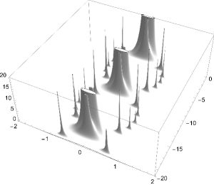
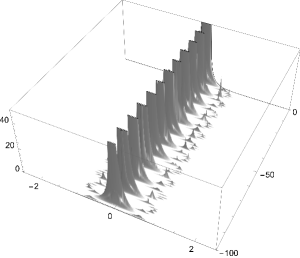
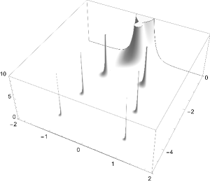
Figure 1: The pole structure of $1/\Delta\tau_{\text{geod}}^{2}$ for $\tau\rightarrow it$ in i) de Sitter ii) Anti-de Sitter and iii) Minkowski spacetime with $a/\sqrt{|\Lambda|}=1.5\sqrt{17}$ and $\Omega/\sqrt{|\Lambda|}=3.5$. For Anti-de Sitter, the parameters chosen satisfy the periodicity conditions (see text) to demonstrate periodicity of poles on the imaginary axis.

VI Detector response

Consider a particle detector modelUnruh (1976); DeWitt (1980); Birrell and Davies (1984) with two energy levels, $\lvert E_{0}\rangle_{d}$ and $\lvert E_{1}\rangle_{d}$ that moves on a stationary trajectory, $x^{i}(\tau)$ as discussed in the previous sections. It interacts with the free real scalar field $\phi$ through an interaction Hamiltonian,

$$H_{\text{int}}=\lambda\,\chi(\tau)\,m(\tau)\,\phi(x^{i}(\tau))$$ (25)

where, $\lambda$ is the coupling constant, $\chi(\tau)$ is the switching function, and $m(\tau)$ is the monopole moment. We consider adiabatic switching for the detector. The detector is in its ground state when the interaction with the scalar field begins and the field is in a state, $\Phi$ and assumes that it satisfies the Hadamard property. To the first order in perturbation theory, the probability of the detector to be in the excited state can be expressed as,

$$P\left(\Delta E\right)=\lambda^{2}\,\lvert\prescript{}{d}{\langle E_{0}\rvert}m(0)\lvert E_{1}\rangle_{d}\rvert^{2}\,\mathcal{F}(\Delta E)$$ (26)

where $\mathcal{F}(\Delta E)$ is the response function that contains the information on the trajectory of the detector and the initial state of the field, and $\Delta E$ is the energy gap of the detector, $E_{1}-E_{0}$. The response function for adiabatic switching is given by,

$$\mathcal{F}\left(\Delta E\right)=\lim_{\epsilon\to 0^{+}}\int_{-\infty}^{\infty}\,\mathrm{d}\tau^{\prime}\,\int_{-\infty}^{\infty}\,\mathrm{d}\tau\,e^{-i\Delta E(\tau-\tau^{\prime})}\,G^{+}_{\epsilon}\left(\tau,\tau^{\prime}\right)$$

Here $G^{+}_{\epsilon}\left(\tau,\tau^{\prime}\right)$ is the pull-back of the Wightman function, $G^{+}_{\epsilon}\left(x^{i}(\tau),x^{i}(\tau^{\prime})\right)$ with $i\varepsilon$ prescription. A more useful quantity is the proper time derivative of the response function known as the instantaneous transition rate. For stationary motion, $G^{+}(\tau,\tau^{\prime})\rightarrow G^{+}(\tau-\tau^{\prime})$ and using the transformation $\tau-\tau^{\prime}=u$ and $\tau^{\prime}=v$, the transition rate can be defined as,

$$\dot{\mathcal{F}}(\Delta E)=\lim_{T\to\infty}\frac{\mathcal{F}(\Delta E)}{T}=\lim_{\epsilon\to 0^{+}}\int_{-\infty}^{\infty}\,\mathrm{d}u\,e^{-i\Delta E\,u}\,G^{+}_{\epsilon}\left(u\right).$$

VI.1 de Sitter spacetime

In de Sitter spacetime we consider a conformally coupled scalar field for simplicity. The Wightman function for the conformally coupled scalar fieldAllen (1985); Garbrecht and Prokopec (2004) is given by,

$$G^{+}\left(x,x^{\prime}\right)=-\frac{\Lambda}{4\pi^{2}y_{\varepsilon}(x,x^{\prime})}$$ (29)

where, $y_{\varepsilon}(x,x^{\prime})$ is the de Sitter invariant distance function with proper $i\varepsilon$ prescription, $y(x,x^{\prime})\rightarrow y(\Delta\tau_{\text{geod}})=-4\sinh^{2}\left(\sqrt{\Lambda}\,\Delta\tau_{\text{geod}}/2\right)$. The transition rate is obtained using numerical methods and is shown in Fig. 2 for different values of acceleration, torsion and curvature length scale. The transition rate approaches the thermal spectrum with temperature, $k_{B}T=\left(\hbar/2\pi\right)\sqrt{a^{2}+\Lambda}$ as $\Omega\rightarrow 0$.

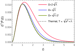
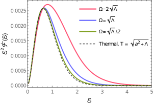
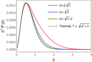
Figure 2: The detector transition rate for a rotating detector in 3+1 de Sitter spacetime is plotted against the dimensionless energy gap, $\Delta E\,\sqrt{\Lambda}=\mathcal{E}$ for different values of acceleration and torsion. Left: $a=2\sqrt{\Lambda}$, Middle: $a=\sqrt{\Lambda}$, Right: $a=\sqrt{\Lambda}/2$. The dashed line corresponds to the thermal spectrum for a linearly accelerating detector in de Sitter.

VI.2 Anti-de Sitter spacetime

For anti-de Sitter spacetime, we again consider a conformally coupled scalar field. The Wightman function is given byAvis et al. (1978),

$$G^{+}_{\text{AdS}_{4}}\left(x,x^{\prime}\right)=-\frac{\Lambda}{4\pi^{2}}\left[\frac{1}{y(x,x^{\prime})}-\frac{\zeta}{y(x,x^{\prime})-2}\right]$$ (30)

where $\zeta\in\{0,-1,1\}$ corresponds to whether the boundary condition specified at infinity is transparent, Dirichlet or Neumann respectively. We will restrict our analysis to transparent boundary conditions for simplicity. In Fig. 3, the response rate of an Unruh-de Witt detector in stationary motion with acceleration and torsion with the parameter values chosen for periodicity in geodesic distance when $\tau\to it$ is illustrated. The transition rate do not correspond to the thermal spectrum due to the presence of complex poles with real parts.

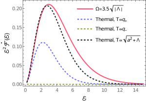
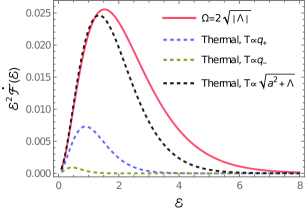
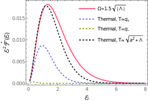
Figure 3: The detector transition rate for 3+1 Anti-de Sitter spacetime with transparent boundary condition plotted against the dimensionless energy gap, $\Delta E\,\sqrt{|\Lambda|}=\mathcal{E}$. Left: $a=1.5\sqrt{17}\sqrt{|\Lambda|}$, Middle: $a=\sqrt{10\,|\Lambda|}$, Right: $a=\sqrt{33\,|\Lambda|}/2$. All the parameter values in this plot satisfy the periodicity condition described in III.2. The dashed lines corresponds to thermal spectrum with different temperature and it is clear that the detector transition rate do not correspond to thermal spectrum even though there is periodicity in geodesic distance for $\tau\to i\,t$.

VII Conclusions and Discussion

We have derived some exact results for uniformly accelerated and rotating detectors in maximally symmetric spacetimes. The key result on which all others are based is the relation between geodesic and proper time intervals between two points on the detector trajectory. Since two-point functions, such as the Wightman function, depend on the former, whereas the detector response involves Fourier transform with respect to the latter, the analytic structure of this relation in the complex (proper time) plane determines the response. In particular, we uncover a periodicity in Euclidean time for certain values of rotation parameter $\Omega$ for $\Lambda<0$, while no such periodicity can be obtained for $\Lambda>0$ or $\Lambda=0$ (the well known case of uniformly rotating detector in Minkowski spacetime). While periodicity of Wightman function in Euclidean time is one of the conditions for thermality, it is not the only one. There are certain analyticity conditions which are also required, as discussed in Ref. Fewster et al. (2016); in particular, $|G^{+}(u)|$ should be bounded by a polynomial, $P(|\text{Re}\,u|)$ in the strip, $S=\{u\in\mathbb{C}\,|-\beta<\text{Im}\,u<0\}$, where $\beta$ is the periodicity. This condition is not satisfied for generic rotational motion due to the presence of additional complex poles with non-zero real parts.

Our results are important as they highlight the subtle role which curvature, howsoever small, can play in determining the nature of response of accelerated, rotating detectors even in the point limit, where equivalence principle would generically imply only perturbative corrections.

In the spirit of the uniformly accelerated (rectilinear) motion discussed in Hari and Kothawala (2021), we also obtained perturbative expansions in curvature for accelerated, rotating detectors in arbitrary curved spacetime (ignoring the derivatives of curvature). However, unlike in Hari and Kothawala (2021), we have not been able to uncover a subset of terms that can be summed to an analytic expression. One obvious reason for this is the complexity of the series in presence of rotation. Besides, our exact results in maximally symmetric spacetimes offer no insights in presence of rotation which brings in an additional spacelike direction that, in turn, brings in more combination of curvature components than can be resolved by looking at dS/AdS, which has just one. We hope, however, to address this in a future work. Any re-summation involving acceleration, curvature and rotation is bound to be of tremendous significance not only in the context of quantum detectors, but also for classical processes in curved spacetimes that involve rotation.

Appendix A Minkowski spacetime

In Minkowski spacetime, the six stationary motions for different values of curvature constants are: i) uniform linear acceleration, ii) circular, iii) cusped, iv) catenary, and v) helical worldlines. Once the trajectory is expressed in terms of the tetrads at the origin, the relation between the geodesic distance and the proper time can be established using, $\Delta\tau^{2}_{\text{geod}}=\eta_{ab}x^{a}(\Delta\tau_{\text{traj}})x^{b}(\Delta\tau_{\text{traj}})$, where the arc length(proper time), $\tau$ is denoted by $\Delta\tau_{\text{traj}}$. Evaluating the derivatives in the Taylor expansion in terms of $u^{i},n^{i},b^{i},d^{i}$ gives,

$$\frac{\mathrm{d}x^{i}}{\mathrm{d}\tau} = u^{i}$$

$$\frac{\mathrm{d}^{2}x^{i}}{\mathrm{d}\tau^{2}} = an^{i}$$

$$\frac{\mathrm{d}^{3}x^{i}}{\mathrm{d}\tau^{3}} = a\Omega b^{i}+a^{2}\frac{\mathrm{d}x^{i}}{\mathrm{d}\tau}$$

$$\frac{\mathrm{d}^{4}x^{i}}{\mathrm{d}\tau^{4}} = a\Omega\lambda d^{i}+(a^{2}-\Omega^{2})\frac{\mathrm{d}^{2}x^{i}}{\mathrm{d}\tau^{2}}$$

$$\frac{\mathrm{d}^{\sf p}x^{i}}{\mathrm{d}\tau^{\sf p}} = (a^{2}-\Omega^{2}-\lambda^{2})\frac{\mathrm{d}^{{\sf p}-2}x^{i}}{\mathrm{d}\tau^{{\sf p}-2}}+a^{2}\lambda^{2}\frac{\mathrm{d}^{{\sf p}-4}x^{i}}{\mathrm{d}\tau^{{\sf p}-4}}$$

for ${\sf p}\geq 5$. Solving the above derivatives using the recurssion relations, we solved the odd and even derivative separately. The series expansion for the trajectory will sum to hyperbolic functions. The trajectory obtained using the solution of the recurssion relation after the summation is given as,

$$x^{i}(\tau) = \frac{2}{q_{-}q_{+}q_{0}^{2}}\left[(a^{2}+\lambda^{2}+\Omega^{2}+q_{0}^{2})q_{-}\sinh{\left(q_{+}\tau\right)}-(a^{2}+\lambda^{2}+\Omega^{2}-q_{0}^{2})q_{+}\sinh{\left(q_{-}\tau\right)}\right]\,u^{i}(0)$$ (31)

$$+\frac{a\,\Omega}{q_{-}q_{+}q_{0}^{2}}\left[q_{-}\sinh{\left(q_{+}\tau\right)}-q_{+}\sinh{\left(q_{-}\tau\right)}\right]\,b^{i}(0)$$

$$+\frac{\Omega}{a\,\lambda\,q_{0}^{2}}\left[q_{+}^{2}\left(\cosh{\left(q_{-}\tau\right)}-1\right)-q_{-}^{2}\left(\cosh{\left(q_{+}\tau\right)}-1\right)\right]\,d^{i}(0)$$

$$+\frac{1}{2aq_{0}^{2}}\left[(a^{2}+\lambda^{2}+\Omega^{2}+q_{0}^{2})\left\{\cosh{\left(q_{+}\tau\right)-1}\right\}-(a^{2}+\lambda^{2}+\Omega^{2}-q_{0}^{2})\left\{\cosh{\left(q_{-}\tau\right)-1}\right\}\right]\,n^{i}(0)$$

Here, $q_{0}:=\left[(a^{2}-\Omega^{2}-\lambda^{2})^{2}+4a^{2}\lambda^{2}\right]^{1/4}$, $q_{\pm}:==(1/\sqrt{2})\sqrt{(a^{2}-\Omega^{2}-\lambda^{2})\pm q_{0}^{2}}$. To find the relation between proper time of the trajectory and the geodesic distance, use $\Delta\tau^{2}_{\text{geod}}=\eta_{ab}x^{a}(\Delta\tau_{\text{traj}})x^{b}(\Delta\tau_{\text{traj}})$, noting that $u^{i}$, $n^{i}$, $b^{i}$, and $d^{i}$ are unit vectors and orthogonal to each other. Then the geodesic distance is,

$$\Delta\tau^{2}_{\text{geod}}=\frac{4}{q_{0}^{2}}\left[\left(1+\frac{(\Omega^{2}+\lambda^{2})}{q_{+}^{2}}\right)\sinh^{2}{}\left(\frac{q_{+}\Delta\tau_{\text{traj}}}{2}\right)-\left(1+\frac{(\Omega^{2}+\lambda^{2})}{q_{-}^{2}}\right)\sinh^{2}{}\left(\frac{q_{-}\Delta\tau_{\text{traj}}}{2}\right)\right]$$ (32)

The above equation is valid for any general stationary motion in Minkowski spacetime. Special cases, such as hyperbolic motion Rindler (1960), is easily obtained by putting torsion and hypertorsion to zero. Other trajectories such as circular motion can be obtained in a similar manner. The different stationary trajectories are as given below:

A.1 Uniform linear acceleration

For uniform linear acceleration or hyperbolic motion, the torsion and hypertorsion will be zero, hence the motion will be in the $u^{i}-n^{i}$ plane. The constants $q_{0},\,q_{-},\,q_{+}$ will reduce to $a,\,0,\,\sqrt{2}a$ respectively. The trajectory will be given by,

$$x^{i}(\tau) = \frac{\sinh{\left(a\tau\right)}}{a}u^{i}(0)+\frac{\left[\cosh{\left(a\tau\right)-1}\right]}{a}n^{i}(0)$$ (33)

The equation for the geodesic distance from the above trajectory simplies to the well know result,

$$\Delta\tau^{2}_{\text{geod}}=\frac{4}{a^{2}}\sinh^{2}\left(\frac{a}{2}\Delta\tau_{\text{traj}}\right)$$ (34)

A.2 Motion with acceleration and torsion

When hypertorsion vanishes and only acceleration and torsion are present, the trajectory will differ according to the values of $a$ and $\Omega$. The general motion with only $a$ and $\Omega$ motion can be expressed using the unit vectors, $u^{i}(0)$, $n^{i}(0)$, and $b^{i}(0)$. The constants $q_{0}$, $q_{-}$, and $q_{+}$ to $\sqrt{a^{2}-\Omega^{2}}$, $0$, and $\sqrt{a^{2}-\Omega^{2}}$ respectively. Applying this to Eq. (32) gives the relation between geodesic distance and proper time. In the case of stationary motion with no hypertorsion, the trajectories are classified into 3 types depending on the magnitudes of acceleration and torsion.

a) Circular motion: When $|\Omega|>|a|$ the motion is bounded(circular). The spatial projection of this motion is circular motion.

b) Cusped motion: For equal magnitudes of acceleration and torsion, the spatial projection of the motion is a cusp.

c) Catenary motion: The spatial projection is catenary when the magnitude of the acceleration is greater than the torsion. The motion is unbounded and the equations for the trajectory and geodesic distance can be obtained by putting $\lambda=0$ in Eq. (31) and Eq. (32) respectively.

A.3 Motion with acceleration, torsion and hypertorsion

The equation for the trajectory is already given in Eq. (31) and the geodesic distance is given in Eq. (32). The equation for the geodesic distance of this general stationary motion is similar to stationary motion in maximally symmetric spacetimes with acceleration and torsion. The spatial projection of this motion is a helix.

References

- Fulling (1973) S. A. Fulling, Physical Review D 7, 2850 (1973).
- Davies (1975) P. C. W. Davies, J. Phys. A8, 609 (1975).
- Unruh (1976) W. Unruh, Physical Review D 14, 870 (1976).
- Deser and Levin (1997) S. Deser and O. Levin, Classical and Quantum Gravity 14, L163 (1997), eprint arXiv:9706018.
- Deser and Levin (1998) S. Deser and O. Levin, Classical and Quantum Gravity 15, L85 (1998), eprint arXiv:9806223.
- Deser and Levin (1999) S. Deser and O. Levin, Physical Review D 59, 064004 (1999), eprint arXiv:9809159.
- Hari and Kothawala (2021) K. Hari and D. Kothawala, Physical Review D 104, 064032 (2021), eprint arXiv:2106.14496.
- Letaw (1981) J. R. Letaw, Physical Review D 23, 1709 (1981).
- Letaw and Pfautsch (1982) J. R. Letaw and J. D. Pfautsch, Journal of Mathematical Physics 23, 425 (1982).
- Letaw and Pfautsch (1981) J. R. Letaw and J. D. Pfautsch, Physical Review D 24, 1491 (1981).
- Weinberg (1972) S. Weinberg, Gravitation and cosmology: principles and applications of the general theory of relativity (1972).
- Hari and Kothawala (2020) K. Hari and D. Kothawala, Physical Review D 101, 124066 (2020), eprint arXiv:2003.10169.
- Hodgkinson and Louko (2012) L. Hodgkinson and J. Louko, Phys. Rev. D 86, 064031 (2012), eprint 1206.2055.
- Banados et al. (1992) M. Banados, C. Teitelboim, and J. Zanelli, Physical Review Letters. 69, 1849 (1992), eprint hep-th/9204099.
- Banados et al. (1993) M. Banados, M. Henneaux, C. Teitelboim, and J. Zanelli, Physical Review D 48, 1506 (1993), [Erratum: Phys.Rev.D 88, 069902 (2013)], eprint gr-qc/9302012.
- Carlip (1995) S. Carlip, Classical and Quantum Gravity 12, 2853 (1995).
- DeWitt (1980) B. S. DeWitt, in General Relativity: An Einstein Centenary Survey (1980), pp. 680–745.
- Birrell and Davies (1984) N. D. Birrell and P. C. W. Davies, Quantum fields in curved space, Cambridge Monographs on Mathematical Physics (Cambridge University Press, 1984).
- Allen (1985) B. Allen, Phys. Rev. D 32, 3136 (1985).
- Garbrecht and Prokopec (2004) B. Garbrecht and T. Prokopec, Class. Quant. Grav. 21, 4993 (2004), eprint gr-qc/0404058.
- Avis et al. (1978) S. J. Avis, C. J. Isham, and D. Storey, Phys. Rev. D 18, 3565 (1978).
- Fewster et al. (2016) C. J. Fewster, B. A. Juárez-Aubry, and J. Louko, Class. Quant. Grav. 33, 165003 (2016), eprint arXiv:1605.01316.
- Rindler (1960) W. Rindler, Physical Review 119, 2082 (1960).