SelfSeg: A Self-supervised Sub-word Segmentation Method for Neural Machine Translation

Abstract.

Sub-word segmentation is an essential pre-processing step for Neural Machine Translation (NMT). Existing work has shown that neural sub-word segmenters are better than Byte-Pair Encoding (BPE), however, they are inefficient as they require parallel corpora, days to train and hours to decode. This paper introduces SelfSeg, a self-supervised neural sub-word segmentation method that is much faster to train/decode and requires only monolingual dictionaries instead of parallel corpora. SelfSeg takes as input a word in the form of a partially masked character sequence, optimizes the word generation probability and generates the segmentation with the maximum posterior probability, which is calculated using a dynamic programming algorithm. The training time of SelfSeg depends on word frequencies, and we explore several word frequency normalization strategies to accelerate the training phase. Additionally, we propose a regularization mechanism that allows the segmenter to generate various segmentations for one word. To show the effectiveness of our approach, we conduct MT experiments in low-, middle- and high-resource scenarios, where we compare the performance of using different segmentation methods. The experimental results demonstrate that on the low-resource ALT dataset, our method achieves more than $1.2$ BLEU score improvement compared with BPE and SentencePiece, and a $1.1$ score improvement over Dynamic Programming Encoding (DPE) and Vocabulary Learning via Optimal Transport (VOLT) on average. The regularization method achieves approximately a $4.3$ BLEU score improvement over BPE and a $1.2$ BLEU score improvement over BPE-dropout, the regularized version of BPE. We also observed significant improvements on IWSLT15 Vi$\rightarrow$En, WMT16 Ro$\rightarrow$En and WMT15 Fi$\rightarrow$En datasets, and competitive results on the WMT14 De$\rightarrow$En and WMT14 Fr$\rightarrow$En datasets. Furthermore, our method is $17.8$x faster during training and up to $36.8$x faster during decoding in a high-resource scenario compared to DPE. We provide extensive analysis, including why monolingual word-level data is enough to train SelfSeg.

1. Introduction

NMT is the most prevalent approach for machine translation (Sutskever et al., 2014; Bahdanau et al., 2014; Vaswani et al., 2017; Gehring et al., 2017) due to its end-to-end nature and its ability to achieve state-of-the-art translations. Early NMT methods consider words as the minimal input unit and use a vocabulary to hold frequent words  (Sutskever et al., 2014; Bahdanau et al., 2014; Luong et al., 2015; Kalchbrenner and Blunsom, 2013). However, they face the out-of-vocabulary (OOV) problem due to the limited size of the vocabulary and the unlimited variety of words in the test data. Even with a very large vocabulary that covers most words in the train set, for morphologically rich languages such as German, there are still $3\%$ of new types of words that appear in the test set  (Jean et al., 2015). This largely hinders the translation quality of sentences with many rare words (Sutskever et al., 2014; Bahdanau et al., 2014).

Sub-word segmentation is dedicated to addressing the OOV problem by segmenting rare words into sub-words or characters that are present in a vocabulary. Frequency-based methods first use a monolingual corpus to build a sub-word vocabulary that contains characters, high-frequency sub-word fragments and common words. During decoding, for each word or sentence, it recursively combines an adjacent fragment pair that occurs most frequently according to the sub-word vocabulary, starting from characters (Sennrich et al., 2016b; Kudo and Richardson, 2018). The main limitation is that these segmentation methods are not optimized for downstream tasks, such as NMT. DPE (He et al., 2020), a recently proposed neural sub-word segmentation approach, views the target sentence as a latent variable whose probability is the sum of the probability of all possible segmentations. The probability of each segmentation is calculated by a transformer model conditioned on the source sentence. It optimizes the target sentence probability in the training phase and outputs the segmentation with maximum posterior probability in the decoding phase. The DPE work also shows the importance of optimizing sub-word segmentation for the MT task. Different from BPE (Sennrich et al., 2016b), it uses parallel data and deploys a neural sequence-to-sequence model for the segmentation. This is a double-edged sword: on one hand, using a sequence-to-sequence neural model enables the segmentation to be aware of all past tokens where BPE does not. Because the NMT decoder is also aware of all past tokens, this segmentation approach may be optimal; on the other hand, it is not practical neither in low-resource scenarios where large parallel corpora are not available, nor in high-resource scenarios where training and decoding take hours to days.

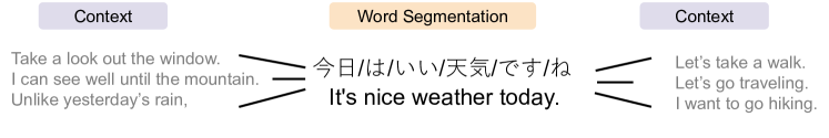
(a) Japanese word segmentation task. The sentence is consistently segmented with different document-level contexts. For the context we show the translated English references only.

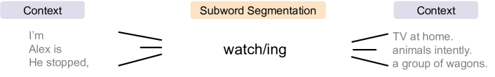
(b) English sub-word segmentation task. The word is consistently segmented with different sentence-level contexts.

Figure 1. Segmentation is a self-contained task where context information is not required.

Leveraging existing large-scale monolingual data through self-supervised learning methods significantly reduces the need for parallel corpora. Predicting masked tokens is a promising task to provide training signals for an encoder that could be fine-tuned for a variety of downstream tasks (Devlin et al., 2019), or an encoder-decoder model which could boost the MT tasks (Song et al., 2019). Although relying on monolingual data obviates the need for parallel corpora, the DPE method will still be slow as entire sequences have to be processed. In order to speed up the model, we propose that words be used instead of sentences. The motivation comes from the examples in Figures 1(a) and  1(b). In Figure 1(a), for a Japanese word segmentation task, the sentence will be consistently segmented in different document-level contexts. It is similar for sub-word segmentation as presented in Figure 1(b), where we don’t need sentence-level information. For example, the word “watching” should be consistently segmented into “watch+ing” no matter which sentence the word is in. This insight can help us go from sentence-level data to word-level data to train the sub-word segmenter, which significantly improves the training and decoding speed, because the training requires only word-level data and one type of word needs to be decoded only once.

Based on these observations, we propose SelfSeg, a sub-word segmenter that trained on monolingual word-level data. It uses a neural model to optimize the word generation probability conditioned on partially masked words, and outputs the segmentation with the maximum posterior probability. The decoding is fast because it only needs to decode each unique word once. To speed up the training phase, we propose a word frequency normalization method that adjusts the frequencies for frequent and rare words. Furthermore, motivated by Provilkov et al. (2020) we also implement a regularization method on top of SelfSeg which provides multiple segmentations of the same word. We conduct experiments for low-, middle- and high-resource language pairs using the corpora from Asian Language Treebank (ALT), IWSLT and WMT. We show that SelfSeg yields segmentations that achieve better translation quality of up to 1.1-1.3 BLEU compared to existing approaches such as BPE (Sennrich et al., 2016b), SentencePiece (Kudo, 2018a), DPE (He et al., 2020) and VOLT (Xu et al., 2021). Additionally, we show that in low-resource settings regularized SelfSeg not only outperforms BPE by 4.3 BLEU but also BPE-dropout (Provilkov et al., 2020) by 1.2 BLEU. We also provide analyses exploring various aspects of SelfSeg. Our contributions are as follows:

• We propose SelfSeg, a neural sub-word segmentation method that relies on only monolingual word-level data with masking strategies, together with word-frequency normalization strategies to speed up the training, and a regularization mechanism.

• Experimental results show significant BLEU score improvements over existing works, as well as a significant increase in training and decoding speed compared to neural approaches such as DPE.

• We provide extensive analysis, including the effect of different masking methods and normalization methods, and why monolingual word-level data is enough to train SelfSeg.

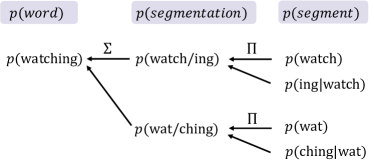
(a) During the training phase model maximizes the probability of one word.

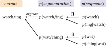
(b) During the decoding phase model seeks the segmentation with the highest probability.

Figure 2. The training and decoding steps for sub-word segmentation.

2. Related Work

In this section, we introduce two categories of sub-word segmentation methods, namely, non-neural and neural methods. In addition, we introduce the prevalent self-supervised learning paradigm.

2.1. Non-Neural Sub-word Segmentation

Initial works on NMT used word-level vocabularies that could only represent the most frequent words, leading to the OOV problem (Sutskever et al., 2014). Character-based or byte-based approaches solve the OOV problem, however, they introduce higher computational complexity and thus translation latency because they generate longer sequences and require deeper-stacked models (often equipped with pre-layer normalization) (Gupta et al., 2019; Kim et al., 2016; Costa-jussà and Fonollosa, 2016; Ling et al., 2015; Luong and Manning, 2016; Cherry et al., 2018; Shaham and Levy, 2021). Fully character-based NMT systems show higher translation quality compared with word-based systems, especially for morphologically rich languages (Kim et al., 2016; Costa-jussà and Fonollosa, 2016; Ling et al., 2015), while a hybrid word-character model shows a larger improvement (Luong and Manning, 2016). A recent study further represents every computerized text as a sequence of bytes via UTF-8 (Shaham and Levy, 2021).

Sub-word segmentation methods address both the OOV problem and the computational cost of the character-based methods, thus becoming an indispensable pre-processing step for modern NMT models (Sennrich et al., 2016b; Provilkov et al., 2020; Wang et al., 2019; Schuster and Nakajima, 2012; Kudo and Richardson, 2018; Kudo, 2018a). Sennrich et al. (2016b) adapt BPE compression algorithm  (Gage, 1994) to the task of sub-word segmentation (in this paper, we use the name BPE to refer specifically to BPE for sub-word segmentation). BPE detects repeated patterns in the text and compresses them into one sub-word. Specifically, it initializes a vocabulary of all types of characters in the training corpora, and adds frequent fragments and words into it. During decoding, a greedy algorithm recursively combines the most frequent adjacent fragment pair in the vocabulary, starting from words that are split into characters. Although not linguistically motivated, the effectiveness may come from the ability of generating shorter sequences (Gallé, 2019). There are several variants of the BPE method, BPE-dropout (Provilkov et al., 2020) is a stochastic or regularized version of BPE where words can be segmented in different ways causing a sentence to have multiple-segmented forms leading to a robust translation model. Subword regularization (Kudo, 2018b) is a regularized version of SentencePiece (Kudo, 2018a) based on a non-neural network unigram language model. VOLT (Xu et al., 2021) finds the best BPE token dictionary with a proper size. Byte-level BPE (BBPE) (Wang et al., 2019) uses bytes as the minimal unit, thus generating a compact vocabulary. WordPiece (WPM) (Schuster and Nakajima, 2012) is similar to BPE where it chooses the adjacent fragment pair that maximizes the likelihood of the training data rather than based on word frequency. Different from BPE which treats space as a special token and thus needs a tokenizer for data in different languages, SentencePiece (SPM) (Kudo and Richardson, 2018) is a language-independent method that treats the input as a raw input stream where space is not a special token. SentencePiece regularization (Kudo, 2018a) is the stochastic version of SPM where it draws multiple segmentations from one sentence to improve the robustness of the model.

The frequency-based methods however are not linguistically motivated, for example, the word “moments” will be segmented as “mom+ents” rather than “moment+s”. Attempts to use a morphological analyzer for sub-word segmentation cannot achieve consistently translation quality improvements (Zhou, 2018; Huck et al., 2017). Furthermore, this method cannot be applied to low-resource languages which lack high-quality morphological analyzers. A recent survey (Mielke et al., 2021) also covers other non-neural methods such as language-specific methods (Koehn and Knight, 2003), bayesian language models (Teh, 2006), and marginalization over multiple possible segmentations (Chan et al., 2016).

2.2. Neural Sub-word Segmentation

Frequency-based methods, such as BPE and SPM, are simple forms of data compression (Gage, 1994) to reduce entropy, which makes the corpus easy to learn and predict (Alikaniotis et al., 2016). While we can optimize the choice of vocabulary to further reduce the entropy (Xu et al., 2021), it is more straightforward to find the segmentation that directly reduces the entropy of a neural model.

Segmentations can be optimized for a neural model to learn and generate by the sequence modeling via segmentations method (Wang et al., 2017). In the training phase, it optimizes the sequence generation probability calculated by the sum of probabilities of all its possible segmentations. In the decoding phase, the segmentation with maximum a posteriori (MAP) is considered the optimal segmentation for each sentence. The sequence modeling via segmentation idea is applied to multiple NLP tasks including word segmentation (Kawakami et al., 2019; Sun and Deng, 2018; Downey et al., 2021), language modeling (Grave et al., 2019), NMT (Kreutzer and Sokolov, 2018), and speech recognition (Wang et al., 2017). During the inference of the language model, utilizing the marginal likelihood with multiple segmentations shows more robust results than one-best-segmentation (Cao and Rimell, 2021). DPE (He et al., 2020) method has applied this sequence modeling and optimization idea to the sub-word segmentation task. They proposed a mixed character-sub-word transformer and apply the dynamic programming (DP) algorithm to accelerate the calculation of sequence modeling. However, segmentation is performed at the sentence-level and conditioned on a sentence in another language. DPE’s parallel corpus requirement makes it unattractive, especially in low-resource settings, which motivated us to rely only on monolingual corpora. However, the mixed character-sub-word transformer is indispensable to our method.

2.3. Self-supervised Machine Learning

Self-supervised methods are becoming popular in machine learning. The advantage of this approach is that it requires only unlabeled (and often monolingual) data, which exists in large quantities. In the NLP field, using monolingual data with denoising objectives has led to significant performance gains in multiple tasks including NMT, question answering (QA) and Multi-Genre Natural Language Inference (MultiNLI) tasks (Devlin et al., 2019; Song et al., 2019; Raffel et al., 2019; Brown et al., 2020; Liu et al., 2019, 2020; Lewis et al., 2020). However, to the best of our knowledge, this approach has not been seriously applied to the sub-word segmentation task yet. Furthermore, the self-supervised method is prevalent in the field of computer vision. There are many works that use unlabeled images to pre-train models (Hinton and Salakhutdinov, 2006; Vincent et al., 2008; Pathak et al., 2016; Doersch et al., 2015; Zhang et al., 2016; Misra et al., 2016; Wei et al., 2018; Vondrick et al., 2018).

3. Methods

We first describe the sequence modeling via segmentation for the sub-word segmentation task as background in Section 3.1. We then describe the proposed segmenter with several masking strategies in Section 3.2, word frequency normalization strategies to accelerate the training speed in Section 3.3, and a regularization mechanism to increase the variety of the generated sub-words in Section 3.4.

3.1. Background: Word Modeling via Sub-word Segmentations

This section describes the word modeling via sub-word segmentation, which is the theoretical foundation of the proposed method.

Let $\bm{x}_{1:T}$ denote a word that comprises $T$ characters, that is $\bm{x}_{1:T}=(x_{1},...,x_{T})$. Let $\bm{a}_{1:\tau_{a}}$ denote one segmentation of $\bm{x}_{1:T}$ that comprises $\tau_{a}$ sub-words, that is $\bm{a}_{1:\tau_{a}}=(a_{1},...,a_{\tau_{a}})$. For each sub-word (or segment) $a_{i}$ in a segmentation $\bm{a}_{1:\tau_{a}}$, it is non-empty substrings of $\bm{x}_{1:T}$ and in a predefined finite size sub-word vocabulary $V$, that is $a_{i}\in V$. The set of all valid segmentations for a word is represented as $S_{x}$, where $\forall\bm{a},\bm{a}\in S_{x}$. Because the sub-word segmentation of one word is not known in advance, the probability of generating one word $\bm{x}_{1:T}$ can be defined as the sum of the probability from all sub-word segmentations in $S_{x}$:

(1) $$\begin{split}p(\bm{x}_{1:T})&=\sum_{\bm{a}_{1:\tau_{a}}\in S_{\bm{x}}}p(\bm{a}_{1:\tau_{a}})\\ &=\sum_{\bm{a}_{1:\tau_{a}}\in S_{\bm{x}}}\prod_{i=1}^{\tau_{a}}p(a_{i}|a_{1},...,a_{i-1}),\end{split}$$

where $p(\bm{x}_{1:T})$ is the probability of the word, $p(\bm{a}_{1:\tau_{a}})$ is the probability of one segmentation and $p(a_{i}|a_{1},...,a_{i-1})$ is the probability of one segment in the segmentation $\bm{a}_{1:\tau_{a}}$, conditioned on previous segments, which is calculated using neural networks such as RNN or Transformer models.

However, for a sequence of length $T$, there are approximately $2^{T}$ types of segmentations. Without using approximation algorithms the time complexity of calculating Eq. (1) will be exponential (O($2^{T}$)), which makes the algorithm too slow thus impractical. To address this, we adopt the mixed character-sub-word transformer model (He et al., 2020) which takes characters as input and generates sub-words as output. The model represent the history information by prefix characters $x_{1},...,x_{j}$ instead of sub-words $a_{1},...,a_{i-1}$, where $j=index(a_{i})-1$. Therefore, we have an approximate word probability:

(2) $$\begin{split}p(\bm{x}_{1:T})=\sum_{\bm{a}_{1:\tau_{a}}\in S_{\bm{x}}}\prod_{i=1}^{\tau_{a}}p(a_{i}|x_{1},...,x_{j})\end{split}$$

In this way, we can calculate the word probability in the time complexity $O(T^{2})$, because there are only $T$ types prefixes as history states, from $x_{1}$, $x_{1}x_{2}$ to $x_{1}...x_{T}$, and only maximum $T$ types of possible next segments from $x_{i}$, $x_{i}x_{i+1}$ to $x_{i}...x_{T}$, suppose the current index is $i$. This is a DP algorithm and helps speed up the segmentation process.

In the training phase, the generation probability of the model for the unsegmented sequences is optimized. Figure 2 provides an example. During the training phase, we can obtain the probability of the word “watching” by summing the probabilities of all possible sub-word segmentations such as “watch+ing” and “wat+ching,” where the probability of each segmentation is the product of the probability of all its segments following the chain rule, calculated by a neural model. The training objective for this unsupervised task is to maximize the generation probability of all words: $\sum_{\bm{x}_{1:T}\in D}\log P(\bm{x}_{1:T})$ where $D$ is the training corpus consisting of the words. For one word $x$ the marginalization $P(\bm{x}_{1:T})$ is the sum of probabilities of all possible segmentations, calculated through Eq. (2). The gradient is calculated automatically through PyTorch and then propagated. The detailed calculation process can be found in Section 3.1 of the sequence modeling work (Wang et al., 2017). In the decoding phase, we calculate the probabilities of all segmentations and then trace the one with maximum probability as the optimal segmentation.

3.2. SelfSeg: Self-supervised Sub-word Segmentation Method

We propose a self-supervised method to train a sub-word segmenter. Given a masked version of one word, the segmenter maximizes the likelihood of all segmentations of the word during training, and selects one segmentation with the highest likelihood during decoding.

The masked version of the word is denoted by $\bm{x}_{M}$. And we maximize the generation probability of word $\bm{x}_{1:T}$ during training by the following objective:

(3) $$\begin{split}\log p(\bm{x}_{1:T}|\bm{x}_{M})=\log\sum_{\bm{a}_{1:\tau_{a}}\in S_{\bm{x}}}\prod_{i=1}^{\tau_{a}}p(a_{i}|\bm{x}_{M},x_{1},...,x_{j})\end{split}$$

We propose the charMASS to generate $\bm{x}_{M}$:

• charMASS: character-level MAsked Sequence-to-Sequence pre-training (charMASS), where half of the consecutive characters in one word are masked. We select the start position of the span from the indexes of the first half of the characters.

In addition, we consider three alternatives:

• subwordMASS: sub-word level MAsked Sequence-to-Sequence pre-training (MASS), where half of the consecutive sub-word segments in one word are masked. We select the start position of the span from the indexes of the first half of the sub-words.

• subwordMASK: strategy used in the MASKed language model, where every sub-word segment is individually masked with a certain probability. We set it to $15\%$ following the BERT paper (Devlin et al., 2019).

• w/o masking: where we set $\bm{x}_{M}$ to the original word $\bm{x}$ without any masks.

Figure 3 illustrates the charMASS method. We directly mask characters in charMASS. However, we generate an initial segmentation using existing sub-word segmentation methods such as BPE (Sennrich et al., 2016b), and mask part of the sub-words. We generate the next sub-word possibilities for each position. The training objective is to maximize the possibility of all paths and in the decoding phase we retrace the optimal path. We create the word-level data by splitting sentence-level data into one word per line format. During decoding, we decode each type of word once which accelerates the decoding phase.

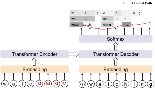
Figure 3. Mixed character-subword transformer. The input of the encoder is one word with masks. The output of the decoder is the possibilities of the next sub-words in each position. We optimize all paths during training and retrace the optimal path during decoding.

3.3. Word Frequency Normalization

We propose frequency normalization methods to speed up the training phase. The motivation is the observation that high-frequency words make up a large part of the training set, such as the words “the” and “is”. However, they can not provide sufficient training signals because most of them are short and non-compound words and tend to stay unsegmented.

Suppose word $w_{i}$ occures $q_{i}$ times in the corpus. And $freq$ is a function that maps $w_{i}$ into $q_{i}$. We propose normalizing function $norm$ acting on the function $freq$ and generate normalized frequency $nq_{i}$ for each word, that is $norm\circ freq(w_{i})=nq_{i}$.

We propose the Threshold as $norm$

• Threshold: $threshold(x)=\lfloor x/d\rfloor$, where we remove words with frequency lower than a threshold $d$ and reduce the frequency for other words. We set $d$ to 10.

In addition, we consider three alternatives:

• Sqrt: $sqrt(x)=\lfloor\sqrt{x}\rfloor$, in this way we reserve all types of words while especially reduce the frequency of high-frequency words.

• Log: $log(x)=\lfloor\log_{2}x\rfloor$, where we also reserve all types of words and cuts the frequency of high-frequency words more strongly.

• One: $One(x)=1$, where we retain only the type information and removes the frequency information.

We create the training data by 1) obtaining a word-frequency table from the corpus, 2) applying the normalizing function and obtaining the normalized word-frequency table, and 3) copying each word $w_{i}$ by $nq_{i}$ times and then shuffle the dataset.

3.4. SelfSeg Regularization

Algorithm 1 shows the proposed SelfSeg-Regularization algorithm that is to increase the variety of the generated sub-words. At each position $i$ of word $\bm{x}$ during decoding, we calculate the scores $\beta_{j}$ of choosing the sub-word $\bm{x}_{j:i}$. Instead of selecting the index $j$ with the highest score, we perform weighted random sampling to draw the next sub-word. As shown in Line $5$, the weights are calculated by feeding the probability of each index $j$ to a softmax function with temperature $t$ to control the diversity. We save the $idx_{i}$ and retrace the segmentation $\bm{z}$ for each run. During decoding, for each type of word, we run the algorithm $N$ times to generate a list of $N$ segmentations.

Input: $\bm{x}$ is a word containing $T$ characters, $V$ is a sub-word vocabulary, $t$ is the temperature hyperparameter.

Output: Segmentation $\bm{z}$

1 for $i\leftarrow 1$ to $T$ do

2       for $j\leftarrow 1$ to $i$ do

3             if $\bm{x}_{j:i}\in V$ then

4                   $\beta_{j}\leftarrow\alpha_{j-1}+\log P(\bm{x}_{j:i}|x_{1},..,x_{j-1})$;

5                  

6            

7      $idx_{i}\leftarrow randomChoice([1,...,i],weights=softmax(\beta/t))$;

8       $\alpha_{i}\leftarrow\beta_{idx_{i}}$;

9      

10$\bm{z}\leftarrow retrace(\bm{idx})$;

11 return $\bm{z}$;

Algorithm 1 SelfSeg-Regularization

4. Experimental Settings

4.1. Datasets

We experimented with low-resource, middle-resource, and high-resource MT settings. The datasets are listed in Table 1, where the size of the vocabulary is set for both the segmenters and NMT models for all methods, if not otherwise specified. We applied Juman++ (Tolmachev et al., 2018) for Japanese, Stanford-tokenizer (Manning et al., 2014) for Chinese and Moses tokenizer (Koehn et al., 2007) to data of all the other languages. We normalized Romanian data and removed diacritics following previous work (Sennrich et al., 2016a).

Table 1. Statistics of the corpora used in the NMT experiments.

Dataset	Train	Valid	Test	Vocab
ALT Asian Langs-En	$18k$	$1,000$	$1,018$	$8k$
IWSLT15 Vi-En	$133k$	$1,553$	$1,268$	$8k$
WMT16 Ro-En	$612k$	$1,999$	$1,999$	$8k$
WMT15 Fi-En	$1.8M$	$1,500$	$1,370$	$8k$
WMT14 De-En	$4.5M$	$45,781$	$3,003$	$8k$
WMT14 Fr-En	$10.0M$	$26,875$	$3,003$	$8k$

Low-resource Setting We used the ALT multi-way parallel dataset (Thu et al., 2016). We used English and $6$ Asian languages: Filipino (Fil), Indonesian (Id), Japanese (Ja), Malay (Ms), Vietnamese (Vi), and simplified Chinese (Zh). The SelfSeg segmenter is applied to only the target language side. Therefore, we train one SelfSeg segmenter using $50,000$ randomly selected English sentences from news commentary corpus for all the Asian language to English directions. We trained a Japanese SelfSeg segmenter using $98k$ Japanese sentences from KFTT dataset (Neubig, 2011) for English to Japanese direction and an Indonesian SelfSeg segmenter using $62k$ Indonesian sentences from the Indonesian news commentary corpus for English to Indonesian direction. We trained one DPE (He et al., 2020) segmenter for each language pair in ALT using the corresponding $18,088$ parallel sentences. We trained BPE (Sennrich et al., 2016b), BPE-dropout (Provilkov et al., 2020) and VOLT (Xu et al., 2021) segmenters using the $18,088$ monolingual sentences in ALT for the corresponding languages.

Middle- and High- Resource Setting We used the IWSLT’15 Vietnamese-English, WMT’16 Romanian-English, WMT’15 Finnish-English, WMT’14 German-English, and WMT’14 French-English corpora. We use the first $10.0$ million parallel sentence pairs in the WMT’14 French-English train set in our experiments. We used English monolingual sentences from the training set of each corpus as the training data for all methods except DPE. For the DPE method, we used the parallel sentences from the train sets following the official implementation, where the input of the encoder is the sentence in the source language, and the predicted output is the sentence in the target language.

4.2. Segmenter Model Settings

BPE, SentencePiece, VOLT, and BPE-dropout For the BPE (Sennrich et al., 2016b) method, we used a widely adopted toolkit with model type as BPE. For SentencePiece, we use unigram language model implemented in the toolkit. For VOLT (Xu et al., 2021), we used the default setting in the official implementation. For BPE-dropout (Provilkov et al., 2020), we apply dynamic dropout for each epoch and with a drop rate of $0.1$ ($0.05$ for English$\rightarrow$Japanese) selected by hyperparameter tunning.

SelfSeg and DPE For SelfSeg, we used charMASS as the masking strategy and Threshold as the word frequency normalization strategy in Section 5. Detailed analysis of the masking strategies and frequency normalization strategies are shown in Section 6. For the SelfSeg and DPE, we used the mixed character-sub-word transformer model with DP algorithm, where the transformer architecture is of $4$ encoder layers and $4$ decoder layers, dropout of $0.3$, inverse sqrt learning rate scheduler with $4,000$ warmup steps, and the dynamic programming cross-entropy criterion as described in the DPE method. We set the number of training epochs to $50$, which is large enough for convergence.Additionally, for the mixed character-sub-word transformer model, the vocabulary $V$ should contain all characters to prevent OOV problems and commonly used sub-words. Here we used a sub-word vocabulary generated by the BPE algorithm (Sennrich et al., 2016b), which satisfies the two conditions, following previous work (He et al., 2020).

SelfSeg-Regularization We set $N$ to 10 and $t$ to $10$ ($t$ to $3$ for English$\rightarrow$Japanese) in Algorithm 1. In the MT experiments, at each epoch, we dynamically generate a segmentation for each sentence in the dataset. For each word in the sentence, we randomly select one of the $N$ segmentations.

Note that DPE, SelfSeg, and SelfSeg-Regularization are used to segment only the target side in the MT experiments. The source-side simply uses BPE data for SelfSeg and BPE-dropout data for the SelfSeg-Regularization. This is because the loss function of the segmenter is to maximize the generation probability. Therefore, these segmentations are effective for the target sentence. This is also studied in the DPE work (He et al., 2020).

4.3. NMT Settings

We used the fairseq framework (Ott et al., 2019) with the Transformer (Vaswani et al., 2017) architecture with $6$ layer encoder (except for Filipino where $4$ encoder layers were sufficient), $6$ layer decoder and $1$ attention head, decided through hyperparameter tuning as suggested by Rubino et al. (2020). Dropout of $0.1$ and label smoothing of $0.1$ is used. We used layer normalization (Lei Ba et al., 2016) for both the encoder and decoder. We used a vocabulary size of $8,000$ for the NMT models. Batch-size is set to $1,024$ tokens. We used the ADAM optimizer (Kingma and Ba, 2014) with betas ($0.9$, $0.98$), warm-up of $4,000$ steps followed by decay, and performed early stopping based on the validation set BLEU. We used a beam size of $12$ and a length penalty of $1.4$ for decoding. We reported sacreBLEU (Post, 2018), METEOR (Banerjee and Lavie, 2005), and BLEURT (Sellam et al., 2020) on detokenized outputs.

5. Results

We report the performance of NMT as well as the training/decoding speed of our methods compared with existing works in this section.

5.1. MT Results

Low-Resource Scenario Tables 2 and 3 show low-resource Asian language to English NMT results. SelfSeg-Regularization achieves the highest BLEU scores among all methods in almost all directions, outperforming the BPE method by $4.31$ BLEU scores on average. Among methods without regularization, proposed SelfSeg outperforms not only frequency-based methods but also neural method DPE. However, we observed that for the Ms$\rightarrow$En and Zh$\rightarrow$En directions, the proposed SelfSeg method is slightly worse (which is not significant) than the BPE method. In particular, we find that both neural methods (DPE and SelfSeg) perform relatively poorly in the Zh$\rightarrow$En direction. Actually, for all directions SelfSeg are better (or worse) than BPE, DPE is also better (or worse) than BPE. Therefore, we assume that for segmentations generated by neural segmenters, the performance do have a correlation with the source language. We will leave the in-depth exploration of this question as future work. We found that adding regularization yields significant BLEU score improvement in the low-resource situation. The SelfSeg-Regularization method substantially improves over BPE. Results of the METEOR and BLEURT evaluation metrics also show similar trends.

Tables 4 and 5 show English to Japanese and Indonesian NMT results of the ALT dataset, English to Romanian results of the WMT16 Ro-En dataset, and the English to Finnish results of the WMT15 Fi-En dataset. In English to Indonesian direction, the SelfSeg-Regularization outperforms all baseline methods substantially. For the English to Japanese direction, the improvement is limited because the average length of the Japanese words in the ALT dataset is short, only $1.87$, resulting in less variety in word segmentation. As a comparison, the average length of English words is $4.54$ and the average length of Indonesian words is $5.50$. This may explain why regularization brings more improvement for English$\rightarrow$Indonesian than English$\rightarrow$Japanese. For the En$\rightarrow$Ro and En$\rightarrow$Fi translation directions, we observed that the SelfSeg performs best among the w/o regularization methods whereas the results of BPE-dropout and SelfSeg-regularization are comparable in terms of the BLEU, METEOR and BLEURT metrics.

Table 2. Low-resource Asian languages to English MT results. The numbers in the table indicate the sacreBLEU scores. We show the average BLEU scores (Avg) and the improvements ($\Delta$) over the BPE method. Methods are separated into without regularization and with regularization. Statistical significance (Koehn, 2004) is indicated by ${}^{\textrm{*}}$ $(p<0.001)$ between the BPE baseline and the proposed methods in each direction.

	Fil$\rightarrow$En	Id$\rightarrow$En	Ja$\rightarrow$En	Ms$\rightarrow$En	Vi$\rightarrow$En	Zh$\rightarrow$En	Avg	$\Delta$
w/o Regularization
BPE (Sennrich et al., 2016b)	$23.09$	$25.70$	$9.42$	$28.19$	$19.94$	$12.21$	$19.76$	$0.00$
SentencePiece (Kudo, 2018a)	$23.71$	$25.49$	$9.94$	$27.72$	$18.58$	$11.74$	$19.53$	$-0.23$
VOLT (Xu et al., 2021)	$22.99$	$25.05$	$10.56$	$27.91$	$21.64$	$11.31$	$19.91$	$0.15$
DPE (He et al., 2020)	$24.04$	$26.66$	$9.93$	$27.89$	$20.06$	$10.72$	$19.88$	$0.13$
SelfSeg	$25.20$${}^{\textrm{*}}$	$27.10$${}^{\textrm{*}}$	$11.39$${}^{\textrm{*}}$	$28.15$	$22.44$${}^{\textrm{*}}$	$12.03$	$21.05$	$1.29$
With Regularization
BPE-dropout (Provilkov et al., 2020)	$28.18$	$28.02$	$12.84$	$31.59$	$23.67$	13.91	$23.04$	$3.13$
SelfSeg-Regularization	$29.94$${}^{\textrm{*}}$	$29.34$${}^{\textrm{*}}$	$15.23$${}^{\textrm{*}}$	$32.31$${}^{\textrm{*}}$	$23.93$${}^{\textrm{*}}$	$13.64$${}^{\textrm{*}}$	$24.07$	$4.31$

Table 3. Low-resource Asian languages to English MT results. The numbers in the table indicate the METEOR (Banerjee and Lavie, 2005)/BLEURT (Sellam et al., 2020) scores. We show the average scores and the improvements ($\Delta$) over the BPE method.

	Fil$\rightarrow$En	Id$\rightarrow$En	Ja$\rightarrow$En	Ms$\rightarrow$En	Vi$\rightarrow$En	Zh$\rightarrow$En	Avg	$\Delta$
w/o Regularization
BPE (Sennrich et al., 2016b)	29.1/45.0	31.1/49.2	20.1/32.4	32.7/52.0	27.6/44.6	22.9/36.9	27.2/43.3	0.0/0.0
SentencePiece (Kudo, 2018a)	29.7/46.1	31.2/48.9	21.0/33.8	32.2/51.0	26.6/42.4	21.6/34.2	27.0/42.7	-0.2/-0.6
VOLT (Xu et al., 2021)	29.2/45.2	31.0/48.8	21.2/34.2	32.5/51.1	28.4/46.6	22.2/35.5	27.4/43.6	0.2/0.2
DPE (He et al., 2020)	29.7/46.5	31.8/50.5	21.1/34.4	32.5/51.6	26.9/43.9	21.5/35.3	27.3/43.7	0.0/0.3
SelfSeg	30.2/47.3	32.0/51.3	21.5/35.3	32.6/52.3	28.4/46.3	22.4/36.5	27.9/44.8	0.6/1.5
With Regularization
BPE-dropout (Provilkov et al., 2020)	32.0/51.1	33.0/52.2	22.8/36.9	34.8/55.8	29.1/48.3	23.6/38.8	29.2/47.2	2.0/3.8
SelfSeg-Regularization	33.2/52.6	33.5/53.9	24.4/40.1	35.0/56.5	29.7/48.7	23.0/38.8	29.8/48.4	2.6/5.1

Table 4. En$\rightarrow$Other language results. En$\rightarrow$Ja and En$\rightarrow$Id directions are from the ALT dataset, En$\rightarrow$Ro direction is from the WMT16 Ro-En dataset and En$\rightarrow$Fi direction is from the WMT15 Fi-En dataset. Statistical significance (Koehn, 2004) is indicated by ${}^{\textrm{*}}$ $(p<0.001)$ between the BPE baseline and the proposed methods in each direction.

	En$\rightarrow$Ja	En$\rightarrow$Id	En$\rightarrow$Ro	En$\rightarrow$Fi
w/o Regularization
BPE (Sennrich et al., 2016b)	12.69	28.08	33.62	15.54
SentencePiece (Kudo, 2018a)	12.58	26.01	33.17	15.75
VOLT (Xu et al., 2021)	13.11	28.46	33.13	15.24
DPE (He et al., 2020)	13.46	29.29	33.71	15.27
SelfSeg	13.26	29.00	33.72	15.85
With Regularization
BPE-dropout (Provilkov et al., 2020)	14.97	30.74	35.48	17.04
SelfSeg-Regularization	14.31${}^{\textrm{*}}$	33.77${}^{\textrm{*}}$	35.47${}^{\textrm{*}}$	16.93${}^{\textrm{*}}$

Table 5. En$\rightarrow$Other language MT results. En$\rightarrow$Ja and En$\rightarrow$Id directions are from the ALT dataset, En$\rightarrow$Ro direction is from the WMT16 Ro-En dataset and En$\rightarrow$Fi direction is from the WMT15 Fi-En dataset. The numbers in the table indicate the METEOR (Banerjee and Lavie, 2005)/BLEURT (Sellam et al., 2020) scores.

	En$\rightarrow$Ja	En$\rightarrow$Id	En$\rightarrow$Ro	En$\rightarrow$Fi
w/o Regularization
BPE (Sennrich et al., 2016b)	24.87/17.94	30.13/46.66	31.19/66.92	19.84/62.02
SentencePiece (Kudo, 2018a)	23.91/17.50	29.29/45.99	31.20/66.38	20.31/63.16
VOLT (Xu et al., 2021)	25.10/18.45	30.31/46.70	31.12/66.02	19.79/61.86
DPE (He et al., 2020)	25.24/18.39	30.76/48.00	31.42/66.69	19.94/62.86
SelfSeg	25.24/18.45	30.59/47.97	31.08/67.30	19.98/62.71
With Regularization
BPE-dropout (Provilkov et al., 2020)	26.00/20.84	31.56/48.66	32.10/69.59	20.90/65.20
SelfSeg-Regularization	25.47/20.65	33.07/50.72	32.04/69.44	21.05/65.61

Middle- and High-Resource Scenario The results for the middle- and high-resource scenarios are presented in Tables  6 and 7. The proposed methods show up to $1.9$ BLEU score improvement, $1.0$ METEOR score improvement and $1.4$ BLEURT score improvement compared with BPE and outperform other baseline methods for all datasets except the high-resource settings WMT14 De$\rightarrow$En and WMT14 Fr$\rightarrow$En. Additionally, the neural methods (DPE and SelfSeg) outperform non-neural methods (BPE and SentencePiece) in most settings.

We find that the effect of subword segmentation on performance becomes marginal as the training data becomes larger. For the WMT14 De$\rightarrow$En and WMT14 Fr$\rightarrow$En directions, we found no improvement over BPE. Additionally, two methods with regularization didn’t show better results than methods without regularization. This is also shown in the DPE work (He et al., 2020) where the improvement is marginal, and the BPE-dropout work (Provilkov et al., 2020) where the dropout hurts the performance for larger datasets. Therefore, one of the limitations of our approach is the small to medium sized MT dataset. Note that we didn’t conduct DPE experiments on the WMT14 De$\rightarrow$En and WMT14 Fr$\rightarrow$En datasets because of excessive computational resource consumption as shown in Section 5.2.

Table 6. Middle- and high-resource MT results with BLEU scores. Statistical significance (Koehn, 2004) is indicated by ${}^{\textrm{*}}$ $(p<0.001)$ between the BPE baseline and the proposed methods in each direction.

	IWSLT15 Vi$\rightarrow$En	WMT16 Ro$\rightarrow$En	WMT15 Fi$\rightarrow$En	WMT14 De$\rightarrow$En	WMT14 Fr$\rightarrow$En
w/o Regularization
BPE (Sennrich et al., 2016b)	27.09	32.54	17.45	31.00	34.97
SentencePiece (Kudo, 2018a)	26.58	31.48	17.74	30.62	34.92
VOLT (Xu et al., 2021)	27.16	31.89	17.25	31.24	35.60
DPE (He et al., 2020)	27.40	33.05	17.51	-	-
SelfSeg	28.19	32.59	18.00	30.82	34.91
With Regularization
BPE-dropout (Provilkov et al., 2020)	28.76	33.59	18.89	30.56	34.38
SelfSeg-Regularization	29.01${}^{\textrm{*}}$	34.01${}^{\textrm{*}}$	19.01${}^{\textrm{*}}$	30.59	34.39

Table 7. Middle- and high-resource MT results. The numbers in the table indicate the METEOR (Banerjee and Lavie, 2005)/BLEURT (Sellam et al., 2020) scores.

	IWSLT15 Vi$\rightarrow$En	WMT16 Ro$\rightarrow$En	WMT15 Fi$\rightarrow$En	WMT14 De$\rightarrow$En	WMT14 Fr$\rightarrow$En
w/o Regularization
BPE (Sennrich et al., 2016b)	31.16/57.75	35.18/61.99	27.06/55.83	34.09/64.66	36.24/67.04
SentencePiece (Kudo, 2018a)	30.63/56.42	34.43/60.64	27.32/56.45	33.49/63.68	36.74/67.46
VOLT (Xu et al., 2021)	30.90/57.13	34.90/61.28	26.73/55.44	34.04/64.60	37.00/67.80
DPE (He et al., 2020)	31.07/57.61	35.47/62.28	27.38/55.96	-	-
SelfSeg	31.46/58.50	35.26/62.44	27.45/56.67	33.54/64.42	36.17/67.31
With Regularization
BPE-dropout (Provilkov et al., 2020)	32.09/59.07	35.73/63.38	28.39/58.43	33.59/64.18	35.95/66.88
SelfSeg-Regularization	32.15/59.17	35.84/63.35	28.11/57.87	33.55/63.72	36.41/66.77

5.2. Training and Decoding Speeds

Figure 4 provides the training speeds and decoding speeds of SelfSeg, BPE and DPE. The training speed of SelfSeg is $17.8$x faster than the DPE method on the WMT’16 Ro-En dataset and $18.7$x faster on the ALT dataset. Although the speed is not as fast as the BPE method, the training process can finish in approximately one hour for a $612k$ size dataset, which is much more acceptable than the DPE method which requires more than one day.

The decoding speed of SelfSeg is $5.9$x on a smaller ALT dataset and $36.8$x on a larger WMT16 Ro-En dataset compared with the DPE method. This is because, according to Zipf’s law, the number of distinct words in a document increases much slower compared with the increment of the total number of words in the document, i.e $\Delta O(\#distinct\ words)\ll\Delta O(\#total\ number\ of\ words)$. As shown in Table 9, for the smaller ALT dataset, DPE needs to decode $14.3$x more tokens than SelfSeg, however, for the larger WMT’16 Ro-En dataset, DPE needs to decode $186.5$x more tokens than SelfSeg. Therefore, the advantage of SelfSeg becomes greater when the corpus becomes bigger because it only needs to decode each distinct word once in the corpus.

The SelfSeg-Regularization method is only applied in the decoding phase, therefore the training time is the same as SelfSeg. During decoding, it generates $N$ segmentations for one word, therefore, the time consumption is $N$ times compared with SelfSeg. When we set $N$ to $10$, the decoding time will still be less than that of DPE.

The speed improvement is important because, in a latency-sensitive scenario, it is important to minimize as many computations as possible. Given that SelfSeg can lead to more intuitive segmentations (as seen in Section 6.6) and better translation than BPE while being significantly faster than DPE, which indicates that the proposed method can be very reliable in a low-latency scenario.

As a supplement, we provide statistics on how many sub-words each sentence contains. As shown in Table 8, there is no significant difference in the number of sub-words in the sentence using different segmentation methods. For the without regularization group, the order is SentencePiece¿SelfSeg¿BPE¿VOLT¿DPE. For the with regularization group, BPE-dropout¿Selfseg-regularization. This shows that the number of sub-words is not a key reason for the speed difference.

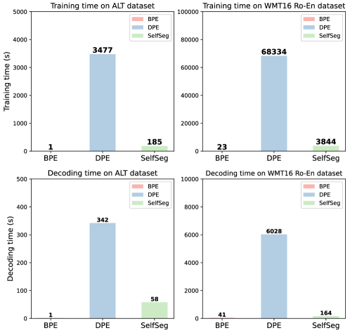
Figure 4. The training and decoding speeds of BPE, DPE, and SelfSeg methods on two datasets.

Table 8. The average number of sub-words in each English sentence by different segmenters.

	ALT Asian Langs$\rightarrow$En	IWSLT15 Vi$\rightarrow$En	WMT16 Ro$\rightarrow$En	WMT15 Fi$\rightarrow$En	WMT14 De$\rightarrow$En	WMT14 Fr$\rightarrow$En
w/o Regularization
BPE (Sennrich et al., 2016b)	34.04	24.80	30.40	26.63	35.41	35.33
SentencePiece (Kudo, 2018a)	41.00	28.15	35.30	29.39	35.79	35.15
VOLT (Xu et al., 2021)	34.04	25.14	29.60	26.03	32.88	32.74
DPE (He et al., 2020)	34.17	24.62	27.44	25.67	-	-
Selfseg	40.31	25.92	34.23	29.19	36.18	36.74
With Regularization
BPE-dropout (Provilkov et al., 2020)	47.20	32.69	44.36	38.82	47.51	49.29
Selfseg-regularization	44.51	32.18	43.50	38.00	46.67	49.25

Table 9. Number of tokens DPE and SelfSeg methods require to decode for each dataset.

	ALT	WMT16 Ro-En
DPE	478k	16M
SelfSeg	33k	70k

6. Analysis

6.1. Masking Strategies

Table 10 shows the performance of using different masking strategies. The charMASS method shows the highest performance, while the performance of subwordMASS is also higher than w/o masking, whereas subwordMASK is slightly worse than w/o masking. This is because the subwordMASK objective is not very suitable for the generation task. Second, charMASS shows higher BLEU scores than subwordMASS. This is because the number of characters in the word is more than the number of sub-words. During training, charMASS can generate more variants of the masked source inputs, which provides more training signals.

Furthermore, results of using 1) different masking ratios and 2) consecutive or non-consecutive masking strategies for charMASS on the Vi$\rightarrow$En direction of the IWSLT15 dataset are shown in Figure 5. We mask $\lfloor ratio*\#chars\rfloor$ characters in each word. For the consecutive strategy, we choose the start point of the masking span from the possible start points randomly. For the non-consecutive strategy, we shuffle a list containing $0$s with the number of masking characters and $1$s with the number of non-masking characters to obtain the masking positions. We found that for both consecutive masking and non-consecutive masking methods, $0.5$ is the best ratio for all settings except SelfSeg-Regularization with consecutive masking, and the performance drops if the masking ratio is very high ($0.9$) or very low ($0.1$). Additionally, there is no significant difference between using consecutive masking and non-consecutive masking strategies.

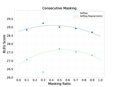
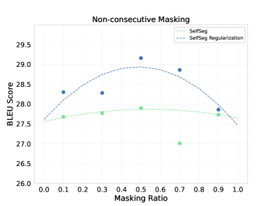
Figure 5. Performance of using different masking ratios and strategies for charMASS. Left: Consecutive masking strategy. Right: Non-consecutive masking strategy. Tested on the Vi$\rightarrow$En direction of the IWSLT15 dataset.

Table 10. The BLEU scores of SelfSeg with different masking strategies.

	Fil$\rightarrow$En	Id$\rightarrow$En	Ja$\rightarrow$En	Ms$\rightarrow$En	Vi$\rightarrow$En	Zh$\rightarrow$En	Avg
charMASS	$25.20$	$27.10$	$11.39$	$28.15$	$22.44$	$12.03$	21.05
subwordMASS	$24.51$	$26.42$	$11.17$	$28.60$	$21.15$	$10.97$	$20.47$
subwordMASK	$23.79$	$25.35$	$10.26$	$28.34$	$21.37$	$12.00$	$20.19$
w/o mask	$24.11$	$26.45$	$10.23$	$28.12$	$21.20$	$11.85$	$20.33$

6.2. Word Frequency Normalization Strategies

Table 11 presents the performance of SelfSeg using different word frequency normalization strategies. We found that 1) using word frequency normalization shows comparable BLEU scores with w/o Norm, and 2) all strategies yield similar results except One, which may come from the large difference in frequency distribution between training and real data. We used subwordMASS strategy here.

Table 11. BLEU scores of SelfSeg with different normalization strategies.

	Fil$\rightarrow$En	Id$\rightarrow$En	Ja$\rightarrow$En	Ms$\rightarrow$En	Vi$\rightarrow$En	Zh$\rightarrow$En	Avg
w/o Norm	$24.51$	$26.42$	$11.17$	$28.60$	$21.15$	$10.97$	20.47
Threshold	$24.74$	$25.86$	$10.42$	$28.82$	$20.90$	$12.06$	20.47
Sqrt	$23.48$	$25.95$	$10.64$	$28.31$	$20.64$	$12.04$	$20.18$
Log	$24.80$	$26.03$	$11.67$	$28.21$	$20.67$	$12.71$	$20.68$
One	$22.89$	$24.80$	$10.25$	$26.82$	$19.87$	$11.56$	$19.37$

6.3. Types of Training Data

We demonstrate that parallel or sentence-level training data is unnecessary and monolingual word-level data is sufficient by both sub-word segmentation results and MT results.

Metrics The MT performance is measured by BLEU scores, and we measure the difference in sub-word segmentation generated by two segmenters on a given dataset through the following metric.

For each word, we define the Word Difference Rate ($DIF_{word}$) by Eq. (4), where $S_{1}$ and $S_{2}$ are sets of sub-word segmentations for the given $word$ generated by two segmenters. $|S|$ is the size of $S$, $nword$ is the frequency of $word$ in the corpus.

(4) $$\begin{split}\mathclap{\mathit{DIF_{word}(S_{1},S_{2},word)}=\frac{\sum_{i=1}^{|S_{1}|}\sum_{j=1}^{|S_{2}|}({\mathit{seg}_{i}\neq\mathit{seg}_{j}})}{\mathit{nword^{2}}}}\end{split}$$

We define Corpus Different Rate ($DIF_{corpus}$) based on $DIF_{word}$ in Eq. (5), where $W$ is a set containing all types of words $word_{i}$ for the given corpus, $|W|$ is the size of $W$.

(5) $$\begin{split}\mathit{DIF_{corpus}(S_{1},S_{2},W)}=\frac{\sum_{i=1}^{|W|}\mathit{DIF_{word}(S_{1},S_{2},word_{i})}*\mathit{nword}_{i}}{\sum_{i=1}^{|W|}\mathit{nword}_{i}}\end{split}$$

Additionally, if $S_{1}=S_{2}$, $DIF_{word}$ and $DIF_{corpus}$ measure the consistency of segmentation of the same word in different sentences by the segmenter.

Settings We calculate $DIF_{corpus}$ among BPE, DPE, SelfSeg-Sentence (using sentence-level data), and SelfSeg on the English part of the IWSLT’15 Vi-En dataset. All four methods use the same vocabulary. The input of SelfSeg-Sentence is a monolingual sentence instead of word during both training and decoding. subwordMASS is used for SelfSeg and SelfSeg-Sentence.

Parallel Data is Not Necessary Tables 12 and 13 present the MT results where using monolingual sentence-level data achieved higher BLEU scores than using parallel data. Figure 6 shows the $DIF_{corpus}$ results. SelfSeg-Sentence gives more consistent segmentations compared with DPE ($0.17\%$ vs. $0.5\%$).

Sentence-level Data is Not Necessary Comparing SelfSeg-Sentence (DPE) and SelfSeg, we can find that SelfSeg using word-level data achieves higher MT performance, showing that word-level data is enough for MT. The DPE work (He et al., 2020) used sentence-level data based on the assumption that one word will be segmented differently in different contexts. However, we found the $DIF_{corpus}(DPE,DPE,IWSLT15)$ is only $0.5\%$ percentage, showing that this assumption is not valid. Furthermore, we divided the words occurring in the dataset into two sets, $W_{high}$ containing high-frequency words ($nword>5$) and $W_{low}$ containing low-frequency words ($nword<=5$). We found $DIF_{corpus}(DPE,DPE,W_{high})$ is only $0.40\%$ whereas $DIF_{corpus}(DPE,DPE,W_{low})$ is $6.14\%$. Even for the $W_{low}$ with high $DIF_{corpus}$, one word should be segmented consistently. For example, DPE segments word jumbled into ju+mble+d and j+umb+led, word mended into me+nded and m+ended, whereas the SelfSeg generates j+umb+l+ed and m+end+ed.

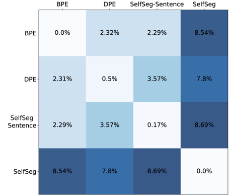
Figure 6. $DIF_{corpus}$ among different segmentation methods on the IWSLT’15 Vi-En dataset.

Table 12. BLEU scores on the ALT dataset using segmenters trained on different types of data. DPE uses parallel sentence-level data, SelfSeg-Sentence uses monolingual sentence-level data, and SelfSeg uses monolingual word-level data.

	Fil$\rightarrow$En	Id$\rightarrow$En	Ja$\rightarrow$En	Ms$\rightarrow$En	Vi$\rightarrow$En	Zh$\rightarrow$En	Avg
BPE (Sennrich et al., 2016b)	$23.09$	$25.70$	$9.42$	$28.19$	$19.94$	$12.21$	$19.76$
DPE (He et al., 2020)	$24.04$	$26.66$	$9.93$	$27.89$	$20.06$	$10.72$	$19.88$
SelfSeg-Sentence	$24.28$	$25.37$	$10.74$	$28.25$	$21.36$	$12.11$	$20.35$
SelfSeg	$24.51$	$26.42$	$11.17$	$28.60$	$21.15$	$10.97$	$20.47$

Table 13. BLEU scores on IWSLT15 Vi$\rightarrow$En dataset with segmenters trained on different types of data.

	IWSLT15 Vi$\rightarrow$En
BPE (Sennrich et al., 2016b)	$27.09$
DPE (He et al., 2020)	$27.40$
SelfSeg-Sentence	$27.79$
SelfSeg	$28.19$

6.4. Sizes of Training Data for SelfSeg

In this section, we investigate the impact of the amount of monolingual data used in the segmenter training. The results are represented in Table 6.4. The amount of English data to train the SelfSeg segmenter varies from $18k$ to $10M$, where the $18k$ setting used the ALT English data, the $50k$ and $532k$ setting used the news commentary corpus, the $4.5M$ setting used the English side of the WMT14 De-En dataset and the $10.0M$ setting used the English side of the WMT14 Fr-En dataset. We find that using more monolingual data brings performance improvement. Especially with $10$M monolingual sentences from WMT14 Fr-En, the improvement reached $1.7$ BLEU score compared with SelfSeg using $18k$ monolingual sentences. Although with more data, the performance of using BPE also improves, the improvement is small compared with that of SelfSeg.

Table 14. Performance of the segmenter model trained on different sizes of the training data. We only have DPE 18k because it uses ALT parallel data.

	Fil$\rightarrow$En	Id$\rightarrow$En	Ja$\rightarrow$En	Ms$\rightarrow$En	Vi$\rightarrow$En	Zh$\rightarrow$En	Avg
Size: 18k
BPE (Sennrich et al., 2016b)	$23.09$	$25.70$	$9.42$	$28.19$	$19.94$	$12.21$	$19.76$
DPE (He et al., 2020)	$24.04$	$26.66$	$9.93$	$27.89$	$20.06$	$10.72$	$19.88$
SelfSeg	$24.11$	$25.85$	$11.11$	$28.73$	$20.68$	$10.46$	$20.16$
Size: 50k
BPE (Sennrich et al., 2016b)	$23.90$	$25.62$	$10.54$	$28.62$	$19.99$	$11.51$	$20.03$
SelfSeg	$24.51$	$26.42$	$11.17$	$28.60$	$21.15$	$10.97$	$20.47$
Size: 532k
BPE (Sennrich et al., 2016b)	$23.71$	$25.68$	$10.59$	$28.53$	$21.57$	$11.04$	20.19
SelfSeg	$23.96$	$26.40$	$9.93$	$28.01$	$20.92$	$11.66$	$20.15$
Size: 4.5M
BPE (Sennrich et al., 2016b)	$23.77$	$26.43$	$10.64$	$27.75$	$22.11$	$11.37$	$20.35$
SelfSeg	$25.60$	$26.45$	$10.09$	$28.57$	$20.23$	$12.22$	20.53
Size: 10.0M
BPE (Sennrich et al., 2016b)	$24.53$	$25.69$	$10.59$	$28.14$	$21.45$	$11.92$	$20.39$
SelfSeg	$26.49$	$27.37$	$11.84$	$29.47$	$23.10$	$12.90$	21.86

6.5. Lightweight SelfSeg Model

We examine a lightweight segmenter model SelfSeg-Light, given that the training data is word-level and on a small scale. The architecture of SelfSeg-Light is a single-layer transformer encoder and a single-layer transformer decoder. As illustrated in Table 15, the performance of SelfSeg-Light is comparable with SelfSeg, which indicates that maybe there is no need to use a large model.

Table 15. BLEU scores of transformers with 4- and 1-layer. With charMASS strategy.

	Fil$\rightarrow$En	Id$\rightarrow$En	Ja$\rightarrow$En	Ms$\rightarrow$En	Vi$\rightarrow$En	Zh$\rightarrow$En	Avg
SelfSeg	$25.20$	$27.10$	$11.39$	$28.15$	$22.44$	$12.03$	$21.05$
SelfSeg-Light	$25.26$	$26.07$	$11.34$	$29.10$	$20.64$	$12.05$	$20.74$

6.6. Segmentation Case Study

In this section, we analyze the segmentation and show why the segmentation generated by our method leads to better performance on the downstream MT task.

Table 16 shows examples of words with different segmentations between the BPE and SelfSeg method on the ALT dataset. We can observe that the BPE method tends to generate high-frequency sub-words, due to the greedy strategy, whereas our SelfSeg, powered by the DP algorithm, tends to generate linguistically intuitive combinations of sub-words for not only frequent words but also rare words. This observation is similar to that by (He et al., 2020). Additionally, Table 17 provides some examples of sub-word segmentations by BPE-dropout (Provilkov et al., 2020) and proposed SelfSeg-Regularization. Both methods yield high diversity of segmentations while the proposed method generates more linguistically intuitive sub-words.

To verify whether our segmentation looks intuitive for the neural models, we trained neural word language models with $Transformer_{base}$ architecture, the same used in the MT experiments, and checked the decoding perplexity. For each segmentation method, we train an English neural word language model on the ALT-train set and test on the ALT-test set segmented by that method. As presented in Table 18, the decoding perplexity of DPE and SelfSeg methods are much lower than that of the BPE method, which we assume is due to the optimization of the log marginal likelihood of the DPE method. From the results of neural LMs, we can infer that when applying our segmentations to MT tasks, the decoder tends to be more certain, as indicated by the low entropy.

Table 16. Examples of sub-word segmentations by different approaches. The frequency of rare words are $<5$, and one-shot words appear only once in the ALT training data.

BPE (Sennrich et al., 2016b)	SelfSeg	BPE (Sennrich et al., 2016b)	SelfSeg
frequent words		rare words
dam + aged	damage + d	d + raf + ting	d + raft + ing
com + ments	comment + s	murd + ered	murder + ed
hous + es	house + s	Net + w + orks	Net + work + s
subsequ + ently	subsequent + ly	aut + h + ored	author + ed
wat + ching	watch + ing	disag + reed	disagree + d
sec + retary	secret + ary	one-shot words
un + k + n + own	un + know + n	reinfor + ces	reinforce + s
refere + es	refer + ee + s	sub + stit + utions	sub + stitution + s
langu + ages	language + s	trad + em + ar + ks	trade + mark + s
you + n + gest	young + est	ris + king	risk + ing
mom + ents	moment + s	Somet + hing	Some + thing

Table 17. Examples of sub-word segmentations by BPE-dropout and SelfSeg-Regularization on the ALT dataset.

BPE-dropout (Provilkov et al., 2020)	SelfSeg-Regularization
frequent words
sub + sequ + ently	subsequent + ly
subsequ + ently	subsequ + ent + ly
s + ub + sequ + ent + l + y	subsequent + l + y
sub + sequ + ently	subsequent + ly
subsequently	subsequ + en + t + ly
rare words
disag + reed	disagree + d
d + is + ag + reed	disag + r + e + ed
disag + re + ed	disag + re + e +d
disag + reed	dis + ag + r + e + ed
d + is + ag + reed	disagree + d
one-shot words
rein + for + ces	reinforce + s
re + in + f + or + ces	reinfor + ces
re + in + for + ces	reinforce + s
rein + for + ces	reinforce + s
re + in + for + ces	reinfor + c + e + s

Table 18. The perplexity of neural LMs. SelfSeg uses subwordMASS strategy.

	PPL per line	PPL per token	# tokens per line
BPE (Sennrich et al., 2016b)	29,688.2	799.4	37.1
DPE (He et al., 2020)	28,498.7	816.1	34.9
SelfSeg	28,714.0	772.2	37.2

7. Conclusion and Future Work

We proposed a novel method SelfSeg for neural sub-word segmentation to improve the performance of NMT and only requires monolingual word-level data. It models the word generation probability through all segmentations and chooses the segmentation with MAP. We propose masking strategies to train the model in a self-supervised manner, word-frequency normalization methods to improve the training speed, and a regularization mechanism that helps to generate segmentations with more variety. Experimental results show that NMT using proposed SelfSeg methods is either comparable to or better than NMT using BPE and DPE in low-resource to high-resource settings And the regularization mechanism achieves a large improvement over baseline methods.

Furthermore, both the training speed and testing speed are more than ten times faster than those of DPE. Analyses show the context agnostic property of the sub-word segmentation, therefore sentence-level training data is not required. Moreover, the segmentations given by the proposed method are more linguistically intuitive as well as easier for the neural decoder to generate as indicated by the low entropy.

Our future work will focus on several directions. First, we are implementing the pre-trained encoder such as BERT/mBERT/BART/mBART on the segmenter. The charMASS method only captures the lexical information and involving semantic information may further improve the quality. Second, we will try to extend the model to multilingual settings. In this way, we only need to train one model to pre-process data of all languages instead of training multiple models for different languages, which can drastically reduce the training time and increases the efficiency of the application. Third, the direction of joint training of the segmenter and the downstream tasks model is also promising, where the segmenter will be aware of the downstream tasks explicitly and be optimized to improve the performance of downstream tasks. Finally, optimizing the vocabulary for sequence generation is necessary. Although the segmentations are optimized for the neural model to generate the word, the possible segments themselves are generated by BPE, which are not optimized for sequence generation.

- (1)
- Alikaniotis et al. (2016) Dimitrios Alikaniotis, Helen Yannakoudakis, and Marek Rei. 2016. Automatic Text Scoring Using Neural Networks. (2016). https://doi.org/10.18653/v1/P16-1068 arXiv:arXiv:1606.04289
- Bahdanau et al. (2014) Dzmitry Bahdanau, Kyunghyun Cho, and Yoshua Bengio. 2014. Neural Machine Translation by Jointly Learning to Align and Translate. arXiv e-prints, Article arXiv:1409.0473 (Sept. 2014), arXiv:1409.0473 pages. arXiv:1409.0473 [cs.CL]
- Banerjee and Lavie (2005) Satanjeev Banerjee and Alon Lavie. 2005. METEOR: An Automatic Metric for MT Evaluation with Improved Correlation with Human Judgments. In Proceedings of the ACL Workshop on Intrinsic and Extrinsic Evaluation Measures for Machine Translation and/or Summarization. Association for Computational Linguistics, Ann Arbor, Michigan, 65–72. https://aclanthology.org/W05-0909
- Brown et al. (2020) Tom B. Brown, Benjamin Mann, Nick Ryder, Melanie Subbiah, Jared Kaplan, Prafulla Dhariwal, Arvind Neelakantan, Pranav Shyam, Girish Sastry, Amanda Askell, Sandhini Agarwal, Ariel Herbert-Voss, Gretchen Krueger, Tom Henighan, Rewon Child, Aditya Ramesh, Daniel M. Ziegler, Jeffrey Wu, Clemens Winter, Christopher Hesse, Mark Chen, Eric Sigler, Mateusz Litwin, Scott Gray, Benjamin Chess, Jack Clark, Christopher Berner, Sam McCandlish, Alec Radford, Ilya Sutskever, and Dario Amodei. 2020. Language Models are Few-Shot Learners. arXiv:arXiv:2005.14165
- Cao and Rimell (2021) Kris Cao and Laura Rimell. 2021. You should evaluate your language model on marginal likelihood over tokenisations. arXiv:arXiv:2109.02550
- Chan et al. (2016) William Chan, Yu Zhang, Quoc Le, and Navdeep Jaitly. 2016. Latent Sequence Decompositions. arXiv:arXiv:1610.03035
- Cherry et al. (2018) Colin Cherry, George Foster, Ankur Bapna, Orhan Firat, and Wolfgang Macherey. 2018. Revisiting Character-Based Neural Machine Translation with Capacity and Compression. In Proceedings of the 2018 Conference on Empirical Methods in Natural Language Processing. Association for Computational Linguistics, Brussels, Belgium, 4295–4305. https://doi.org/10.18653/v1/D18-1461
- Costa-jussà and Fonollosa (2016) Marta R. Costa-jussà and José A. R. Fonollosa. 2016. Character-based Neural Machine Translation. In Proceedings of the 54th Annual Meeting of the Association for Computational Linguistics (Volume 2: Short Papers). Association for Computational Linguistics, Berlin, Germany, 357–361. https://doi.org/10.18653/v1/P16-2058
- Devlin et al. (2019) Jacob Devlin, Ming-Wei Chang, Kenton Lee, and Kristina Toutanova. 2019. BERT: Pre-training of Deep Bidirectional Transformers for Language Understanding. In Proceedings of the 2019 Conference of the North American Chapter of the Association for Computational Linguistics: Human Language Technologies, Volume 1 (Long and Short Papers). Association for Computational Linguistics, Minneapolis, Minnesota, 4171–4186. https://doi.org/10.18653/v1/N19-1423
- Doersch et al. (2015) Carl Doersch, Abhinav Gupta, and Alexei A. Efros. 2015. Unsupervised Visual Representation Learning by Context Prediction. In Proceedings of the IEEE International Conference on Computer Vision (ICCV).
- Downey et al. (2021) C. M. Downey, Fei Xia, Gina-Anne Levow, and Shane Steinert-Threlkeld. 2021. A Masked Segmental Language Model for Unsupervised Natural Language Segmentation. arXiv:arXiv:2104.07829
- Gage (1994) Philip Gage. 1994. A new algorithm for data compression. C Users Journal 12, 2 (1994), 23–38.
- Gallé (2019) Matthias Gallé. 2019. Investigating the Effectiveness of BPE: The Power of Shorter Sequences. In Proceedings of the 2019 Conference on Empirical Methods in Natural Language Processing and the 9th International Joint Conference on Natural Language Processing (EMNLP-IJCNLP). Association for Computational Linguistics, Hong Kong, China, 1375–1381. https://doi.org/10.18653/v1/D19-1141
- Gehring et al. (2017) Jonas Gehring, Michael Auli, David Grangier, Denis Yarats, and Yann N. Dauphin. 2017. Convolutional Sequence to Sequence Learning. In Proceedings of the 34th International Conference on Machine Learning - Volume 70 (Sydney, NSW, Australia) (ICML’17). JMLR.org, 1243–1252.
- Grave et al. (2019) Edouard Grave, Sainbayar Sukhbaatar, Piotr Bojanowski, and Armand Joulin. 2019. Training Hybrid Language Models by Marginalizing over Segmentations. In Proceedings of the 57th Annual Meeting of the Association for Computational Linguistics. Association for Computational Linguistics, Florence, Italy, 1477–1482. https://doi.org/10.18653/v1/P19-1143
- Gupta et al. (2019) Rohit Gupta, Laurent Besacier, Marc Dymetman, and Matthias Gallé. 2019. Character-based NMT with Transformer. arXiv:arXiv:1911.04997
- He et al. (2020) Xuanli He, Gholamreza Haffari, and Mohammad Norouzi. 2020. Dynamic Programming Encoding for Subword Segmentation in Neural Machine Translation. In Proceedings of the 58th Annual Meeting of the Association for Computational Linguistics. Association for Computational Linguistics, Online, 3042–3051. https://doi.org/10.18653/v1/2020.acl-main.275
- Hinton and Salakhutdinov (2006) G. E. Hinton and R. R. Salakhutdinov. 2006. Reducing the Dimensionality of Data with Neural Networks. Science 313, 5786 (2006), 504–507. https://doi.org/10.1126/science.1127647 arXiv:https://science.sciencemag.org/content/313/5786/504.full.pdf
- Huck et al. (2017) Matthias Huck, Simon Riess, and Alexander Fraser. 2017. Target-side Word Segmentation Strategies for Neural Machine Translation. In Proceedings of the Second Conference on Machine Translation. Association for Computational Linguistics, Copenhagen, Denmark, 56–67. https://doi.org/10.18653/v1/W17-4706
- Jean et al. (2015) Sébastien Jean, Kyunghyun Cho, Roland Memisevic, and Yoshua Bengio. 2015. On Using Very Large Target Vocabulary for Neural Machine Translation. In Proceedings of the 53rd Annual Meeting of the Association for Computational Linguistics and the 7th International Joint Conference on Natural Language Processing (Volume 1: Long Papers). Association for Computational Linguistics, Beijing, China, 1–10. https://doi.org/10.3115/v1/P15-1001
- Kalchbrenner and Blunsom (2013) Nal Kalchbrenner and Phil Blunsom. 2013. Recurrent Continuous Translation Models. In Proceedings of the 2013 Conference on Empirical Methods in Natural Language Processing. Association for Computational Linguistics, Seattle, Washington, USA, 1700–1709. https://aclanthology.org/D13-1176
- Kawakami et al. (2019) Kazuya Kawakami, Chris Dyer, and Phil Blunsom. 2019. Learning to Discover, Ground and Use Words with Segmental Neural Language Models. In Proceedings of the 57th Annual Meeting of the Association for Computational Linguistics. Association for Computational Linguistics, Florence, Italy, 6429–6441. https://doi.org/10.18653/v1/P19-1645
- Kim et al. (2016) Yoon Kim, Yacine Jernite, David Sontag, and Alexander Rush. 2016. Character-Aware Neural Language Models. Proceedings of the AAAI Conference on Artificial Intelligence 30, 1 (Mar. 2016). https://ojs.aaai.org/index.php/AAAI/article/view/10362
- Kingma and Ba (2014) Diederik P. Kingma and Jimmy Ba. 2014. Adam: A Method for Stochastic Optimization. arXiv e-prints, Article arXiv:1412.6980 (Dec. 2014), arXiv:1412.6980 pages. arXiv:1412.6980 [cs.LG]
- Koehn (2004) Philipp Koehn. 2004. Statistical Significance Tests for Machine Translation Evaluation. In Proceedings of the 2004 Conference on Empirical Methods in Natural Language Processing. Association for Computational Linguistics, Barcelona, Spain, 388–395. https://www.aclweb.org/anthology/W04-3250
- Koehn et al. (2007) Philipp Koehn, Hieu Hoang, Alexandra Birch, Chris Callison-Burch, Marcello Federico, Nicola Bertoldi, Brooke Cowan, Wade Shen, Christine Moran, Richard Zens, Chris Dyer, Ondřej Bojar, Alexandra Constantin, and Evan Herbst. 2007. Moses: Open Source Toolkit for Statistical Machine Translation. In Proceedings of the 45th Annual Meeting of the Association for Computational Linguistics Companion Volume Proceedings of the Demo and Poster Sessions. Association for Computational Linguistics, Prague, Czech Republic, 177–180. https://www.aclweb.org/anthology/P07-2045
- Koehn and Knight (2003) Philipp Koehn and Kevin Knight. 2003. Empirical Methods for Compound Splitting. In 10th Conference of the European Chapter of the Association for Computational Linguistics. Association for Computational Linguistics, Budapest, Hungary. https://aclanthology.org/E03-1076
- Kreutzer and Sokolov (2018) Julia Kreutzer and Artem Sokolov. 2018. Learning to Segment Inputs for NMT Favors Character-Level Processing. arXiv:arXiv:1810.01480
- Kudo (2018a) Taku Kudo. 2018a. Subword Regularization: Improving Neural Network Translation Models with Multiple Subword Candidates. In Proceedings of the 56th Annual Meeting of the Association for Computational Linguistics (Volume 1: Long Papers). Association for Computational Linguistics, Melbourne, Australia, 66–75. https://doi.org/10.18653/v1/P18-1007
- Kudo (2018b) Taku Kudo. 2018b. Subword Regularization: Improving Neural Network Translation Models with Multiple Subword Candidates. arXiv:arXiv:1804.10959
- Kudo and Richardson (2018) Taku Kudo and John Richardson. 2018. SentencePiece: A simple and language independent subword tokenizer and detokenizer for Neural Text Processing. In Proceedings of the 2018 Conference on Empirical Methods in Natural Language Processing: System Demonstrations. Association for Computational Linguistics, Brussels, Belgium, 66–71. https://doi.org/10.18653/v1/D18-2012
- Lei Ba et al. (2016) Jimmy Lei Ba, Jamie Ryan Kiros, and Geoffrey E. Hinton. 2016. Layer Normalization. arXiv e-prints, Article arXiv:1607.06450 (July 2016), arXiv:1607.06450 pages. arXiv:1607.06450 [stat.ML]
- Lewis et al. (2020) Mike Lewis, Yinhan Liu, Naman Goyal, Marjan Ghazvininejad, Abdelrahman Mohamed, Omer Levy, Veselin Stoyanov, and Luke Zettlemoyer. 2020. BART: Denoising Sequence-to-Sequence Pre-training for Natural Language Generation, Translation, and Comprehension. In Proceedings of the 58th Annual Meeting of the Association for Computational Linguistics. Association for Computational Linguistics, Online, 7871–7880. https://doi.org/10.18653/v1/2020.acl-main.703
- Ling et al. (2015) Wang Ling, Isabel Trancoso, Chris Dyer, and Alan W Black. 2015. Character-based Neural Machine Translation. arXiv:arXiv:1511.04586
- Liu et al. (2020) Yinhan Liu, Jiatao Gu, Naman Goyal, Xian Li, Sergey Edunov, Marjan Ghazvininejad, Mike Lewis, and Luke Zettlemoyer. 2020. Multilingual Denoising Pre-training for Neural Machine Translation. Transactions of the Association for Computational Linguistics 8 (11 2020), 726–742. https://doi.org/10.1162/tacl_a_00343 arXiv:https://direct.mit.edu/tacl/article-pdf/doi/10.1162/tacl_a_00343/1923401/tacl_a_00343.pdf
- Liu et al. (2019) Yinhan Liu, Myle Ott, Naman Goyal, Jingfei Du, Mandar Joshi, Danqi Chen, Omer Levy, Mike Lewis, Luke Zettlemoyer, and Veselin Stoyanov. 2019. RoBERTa: A Robustly Optimized BERT Pretraining Approach. arXiv:arXiv:1907.11692
- Luong and Manning (2016) Minh-Thang Luong and Christopher D. Manning. 2016. Achieving Open Vocabulary Neural Machine Translation with Hybrid Word-Character Models. arXiv:arXiv:1604.00788
- Luong et al. (2015) Thang Luong, Ilya Sutskever, Quoc Le, Oriol Vinyals, and Wojciech Zaremba. 2015. Addressing the Rare Word Problem in Neural Machine Translation. In Proceedings of the 53rd Annual Meeting of the Association for Computational Linguistics and the 7th International Joint Conference on Natural Language Processing (Volume 1: Long Papers). Association for Computational Linguistics, Beijing, China, 11–19. https://doi.org/10.3115/v1/P15-1002
- Manning et al. (2014) Christopher Manning, Mihai Surdeanu, John Bauer, Jenny Finkel, Steven Bethard, and David McClosky. 2014. The Stanford CoreNLP Natural Language Processing Toolkit. In Proceedings of 52nd Annual Meeting of the Association for Computational Linguistics: System Demonstrations. Association for Computational Linguistics, Baltimore, Maryland, 55–60. https://doi.org/10.3115/v1/P14-5010
- Mielke et al. (2021) Sabrina J. Mielke, Zaid Alyafeai, Elizabeth Salesky, Colin Raffel, Manan Dey, Matthias Gallé, Arun Raja, Chenglei Si, Wilson Y. Lee, Benoît Sagot, and Samson Tan. 2021. Between words and characters: A Brief History of Open-Vocabulary Modeling and Tokenization in NLP. arXiv:arXiv:2112.10508
- Misra et al. (2016) Ishan Misra, C. Lawrence Zitnick, and Martial Hebert. 2016. Shuffle and Learn: Unsupervised Learning using Temporal Order Verification. arXiv:arXiv:1603.08561
- Neubig (2011) Graham Neubig. 2011. The Kyoto Free Translation Task. http://www.phontron.com/kftt.
- Ott et al. (2019) Myle Ott, Sergey Edunov, Alexei Baevski, Angela Fan, Sam Gross, Nathan Ng, David Grangier, and Michael Auli. 2019. fairseq: A Fast, Extensible Toolkit for Sequence Modeling. In Proceedings of the 2019 Conference of the North American Chapter of the Association for Computational Linguistics (Demonstrations). Association for Computational Linguistics, Minneapolis, Minnesota, 48–53. https://doi.org/10.18653/v1/N19-4009
- Pathak et al. (2016) Deepak Pathak, Philipp Krahenbuhl, Jeff Donahue, Trevor Darrell, and Alexei A. Efros. 2016. Context Encoders: Feature Learning by Inpainting. CVPR 2016. (2016). arXiv:arXiv:1604.07379
- Post (2018) Matt Post. 2018. A Call for Clarity in Reporting BLEU Scores. In Proceedings of the Third Conference on Machine Translation: Research Papers. Association for Computational Linguistics, Belgium, Brussels, 186–191. https://www.aclweb.org/anthology/W18-6319
- Provilkov et al. (2020) Ivan Provilkov, Dmitrii Emelianenko, and Elena Voita. 2020. BPE-Dropout: Simple and Effective Subword Regularization. In Proceedings of the 58th Annual Meeting of the Association for Computational Linguistics. Association for Computational Linguistics, Online, 1882–1892. https://doi.org/10.18653/v1/2020.acl-main.170
- Raffel et al. (2019) Colin Raffel, Noam Shazeer, Adam Roberts, Katherine Lee, Sharan Narang, Michael Matena, Yanqi Zhou, Wei Li, and Peter J. Liu. 2019. Exploring the Limits of Transfer Learning with a Unified Text-to-Text Transformer. arXiv:arXiv:1910.10683
- Rubino et al. (2020) Raphael Rubino, Benjamin Marie, Raj Dabre, Atsushi Fujita, Masao Utiyama, and Eiichiro Sumita. 2020. Extremely low-resource neural machine translation for Asian languages. Mach. Transl. 34, 4 (2020), 347–382. https://doi.org/10.1007/s10590-020-09258-6
- Schuster and Nakajima (2012) M. Schuster and K. Nakajima. 2012. Japanese and Korean voice search. In 2012 IEEE International Conference on Acoustics, Speech and Signal Processing (ICASSP). 5149–5152. https://ieeexplore.ieee.org/abstract/document/6289079
- Sellam et al. (2020) Thibault Sellam, Dipanjan Das, and Ankur Parikh. 2020. BLEURT: Learning Robust Metrics for Text Generation. In Proceedings of the 58th Annual Meeting of the Association for Computational Linguistics. Association for Computational Linguistics, Online, 7881–7892. https://doi.org/10.18653/v1/2020.acl-main.704
- Sennrich et al. (2016a) Rico Sennrich, Barry Haddow, and Alexandra Birch. 2016a. Edinburgh Neural Machine Translation Systems for WMT 16. In Proceedings of the First Conference on Machine Translation: Volume 2, Shared Task Papers. Association for Computational Linguistics, Berlin, Germany, 371–376. https://doi.org/10.18653/v1/W16-2323
- Sennrich et al. (2016b) Rico Sennrich, Barry Haddow, and Alexandra Birch. 2016b. Neural Machine Translation of Rare Words with Subword Units. In Proceedings of the 54th Annual Meeting of the Association for Computational Linguistics (Volume 1: Long Papers). Association for Computational Linguistics, Berlin, Germany, 1715–1725. https://doi.org/10.18653/v1/P16-1162
- Shaham and Levy (2021) Uri Shaham and Omer Levy. 2021. Neural Machine Translation without Embeddings. In Proceedings of the 2021 Conference of the North American Chapter of the Association for Computational Linguistics: Human Language Technologies. Association for Computational Linguistics, Online, 181–186. https://doi.org/10.18653/v1/2021.naacl-main.17
- Song et al. (2019) Kaitao Song, Xu Tan, Tao Qin, Jianfeng Lu, and Tie-Yan Liu. 2019. MASS: Masked Sequence to Sequence Pre-training for Language Generation. arXiv e-prints, Article arXiv:1905.02450 (May 2019), arXiv:1905.02450 pages. arXiv:1905.02450 [cs.CL]
- Sun and Deng (2018) Zhiqing Sun and Zhi-Hong Deng. 2018. Unsupervised Neural Word Segmentation for Chinese via Segmental Language Modeling. In Proceedings of the 2018 Conference on Empirical Methods in Natural Language Processing. Association for Computational Linguistics, Brussels, Belgium, 4915–4920. https://doi.org/10.18653/v1/D18-1531
- Sutskever et al. (2014) Ilya Sutskever, Oriol Vinyals, and Quoc V Le. 2014. Sequence to Sequence Learning with Neural Networks. In Advances in Neural Information Processing Systems 27, Z. Ghahramani, M. Welling, C. Cortes, N. D. Lawrence, and K. Q. Weinberger (Eds.). Curran Associates, Inc., 3104–3112. http://papers.nips.cc/paper/5346-sequence-to-sequence-learning-with-neural-networks.pdf
- Teh (2006) Yee Whye Teh. 2006. A Hierarchical Bayesian Language Model Based On Pitman-Yor Processes. In Proceedings of the 21st International Conference on Computational Linguistics and 44th Annual Meeting of the Association for Computational Linguistics. Association for Computational Linguistics, Sydney, Australia, 985–992. https://doi.org/10.3115/1220175.1220299
- Thu et al. (2016) Ye Kyaw Thu, Win Pa Pa, Masao Utiyama, Andrew Finch, and Eiichiro Sumita. 2016. Introducing the Asian Language Treebank (ALT). In Proceedings of the Tenth International Conference on Language Resources and Evaluation (LREC’16). European Language Resources Association (ELRA), Portorož, Slovenia, 1574–1578. https://www.aclweb.org/anthology/L16-1249
- Tolmachev et al. (2018) Arseny Tolmachev, Daisuke Kawahara, and Sadao Kurohashi. 2018. Juman++: A Morphological Analysis Toolkit for Scriptio Continua. In Proceedings of the 2018 Conference on Empirical Methods in Natural Language Processing: System Demonstrations. Association for Computational Linguistics, Brussels, Belgium, 54–59. https://doi.org/10.18653/v1/D18-2010
- Vaswani et al. (2017) Ashish Vaswani, Noam Shazeer, Niki Parmar, Jakob Uszkoreit, Llion Jones, Aidan N Gomez, Ł ukasz Kaiser, and Illia Polosukhin. 2017. Attention is All you Need. In Advances in Neural Information Processing Systems, I. Guyon, U. V. Luxburg, S. Bengio, H. Wallach, R. Fergus, S. Vishwanathan, and R. Garnett (Eds.), Vol. 30. Curran Associates, Inc. https://proceedings.neurips.cc/paper/2017/file/3f5ee243547dee91fbd053c1c4a845aa-Paper.pdf
- Vincent et al. (2008) Pascal Vincent, Hugo Larochelle, Yoshua Bengio, and Pierre-Antoine Manzagol. 2008. Extracting and Composing Robust Features with Denoising Autoencoders. In Proceedings of the 25th International Conference on Machine Learning (Helsinki, Finland) (ICML ’08). Association for Computing Machinery, New York, NY, USA, 1096–1103. https://doi.org/10.1145/1390156.1390294
- Vondrick et al. (2018) Carl Vondrick, Abhinav Shrivastava, Alireza Fathi, Sergio Guadarrama, and Kevin Murphy. 2018. Tracking Emerges by Colorizing Videos. In Proceedings of the European Conference on Computer Vision (ECCV).
- Wang et al. (2019) Changhan Wang, Kyunghyun Cho, and Jiatao Gu. 2019. Neural Machine Translation with Byte-Level Subwords. arXiv:arXiv:1909.03341
- Wang et al. (2017) Chong Wang, Yining Wang, Po-Sen Huang, Abdelrahman Mohamed, Dengyong Zhou, and Li Deng. 2017. Sequence Modeling via Segmentations. arXiv:arXiv:1702.07463
- Wei et al. (2018) Donglai Wei, Joseph J. Lim, Andrew Zisserman, and William T. Freeman. 2018. Learning and Using the Arrow of Time. In Proceedings of the IEEE Conference on Computer Vision and Pattern Recognition (CVPR).
- Xu et al. (2021) Jingjing Xu, Hao Zhou, Chun Gan, Zaixiang Zheng, and Lei Li. 2021. Vocabulary Learning via Optimal Transport for Neural Machine Translation. In Proceedings of the 59th Annual Meeting of the Association for Computational Linguistics and the 11th International Joint Conference on Natural Language Processing (Volume 1: Long Papers). Association for Computational Linguistics, Online, 7361–7373. https://doi.org/10.18653/v1/2021.acl-long.571
- Zhang et al. (2016) Richard Zhang, Phillip Isola, and Alexei A Efros. 2016. Colorful image colorization. In European conference on computer vision. Springer, 649–666.
- Zhou (2018) Giulio Zhou. 2018. Morphological Zero-Shot Neural Machine Translation. University of Edinburgh.