Abstract

Distributed learning is commonly used for training deep learning models, especially large models. In distributed learning, manual parallelism (MP) methods demand considerable human effort and have limited flexibility. Hence, automatic parallelism (AP) methods have recently been proposed for automating the parallel strategy optimization process. Existing AP methods suffer from sub-optimal solutions because they do not jointly optimize the two categories of parallel strategies (i.e., inter-layer parallelism and intra-layer parallelism). In this paper, we propose a novel AP method called UniAP, which unifies inter- and intra-layer automatic parallelism by mixed integer quadratic programming. To the best of our knowledge, UniAP is the first parallel method that can jointly optimize the two categories of parallel strategies to find an optimal solution. Experimental results show that UniAP outperforms state-of-the-art methods by up to 1.71$\times$ in throughput and reduces strategy optimization time by up to 107$\times$ across five Transformer-based models.

1 Introduction

Deep learning models have demonstrated promising performance across many domains. For example, deep learning models such as BERT (Devlin et al., 2019), GPT-3 (Brown et al., 2020) and T5 (Raffel et al., 2020) achieve state-of-the-art (SOTA) performance on many natural language processing (NLP) tasks. For computer vision (CV), deep learning models such as ViT (Dosovitskiy et al., 2021) and Swin Transformer (Liu et al., 2021) achieve good accuracy on multiple tasks.

Distributed learning (also called parallel learning) on clusters with several machines or GPUs is commonly used for training deep learning models, especially for some large models with billions of parameters (Brown et al., 2020; Touvron et al., 2023a; b). Several parallel strategies, including pipeline parallelism (PP), data parallelism (DP), tensor parallelism (TP), and fully sharded data parallelism (FSDP), have been proposed for distributed learning. These parallel strategies can be divided into two main categories: inter-layer parallelism and intra-layer parallelism. Inter-layer parallelism (Huang et al., 2019; Narayanan et al., 2019; 2021a; Fan et al., 2021; Li & Hoefler, 2021; Lepikhin et al., 2021; Du et al., 2022; Fedus et al., 2022), which includes PP, partitions the model into disjoint sets without partitioning tensors in each layer. Intra-layer parallelism (Li et al., 2020; Rasley et al., 2020; Narayanan et al., 2021b; FairScale authors, 2021), which includes DP, TP, and FSDP, partitions tensors in a layer along one or more axes.

The parallel method in one specific distributed learning method or system typically adopts one parallel strategy or a combination of several parallel strategies. Existing parallel methods can be divided into two categories: manual parallelism (MP) methods and automatic parallelism (AP) methods. In MP methods  (Shazeer et al., 2018; Narayanan et al., 2021b; Xu et al., 2021), one or several parallel strategies are manually optimized by researchers or developers. MP methods require extensive domain knowledge in deep learning models and hardware architectures. With the rapid development of deep learning models and the increasing diversity of modern hardware architectures (Flynn, 1966; 1972), MP methods demand considerable human effort and have limited flexibility.

To address the two limitations of MP methods, AP methods (Narayanan et al., 2019; He et al., 2021; Zheng et al., 2022) have recently been proposed for automating the parallel strategy optimization process. Although existing AP methods have achieved promising progress, they optimize the two categories of parallel strategies separately rather than jointly. More specifically, some methods optimize only one category of parallel strategies (Jia et al., 2018; Wang et al., 2019; Jia et al., 2019; Schaarschmidt et al., 2021; Zhao et al., 2022; Cai et al., 2022; Liu et al., 2023), and the others optimize inter- and intra-layer parallelism hierarchically (Narayanan et al., 2019; Tarnawski et al., 2020; 2021; Fan et al., 2021; He et al., 2021; Zheng et al., 2022). Hence, existing AP methods suffer from sub-optimal solutions.

In this paper, we propose a novel AP method called UniAP for distributed learning. The contributions of UniAP are outlined as follows:

• UniAP unifies inter- and intra-layer automatic parallelism by mixed integer quadratic programming (MIQP) (Lazimy, 1982).

• To the best of our knowledge, UniAP is the first parallel method that can jointly optimize the two categories of parallel strategies to find an optimal solution.

• Experimental results show that UniAP outperforms state-of-the-art methods by up to 1.71$\times$ in throughput and reduces strategy optimization time by up to 107$\times$ across five Transformer-based models.

2 Background

2.1 Parallel Strategy

Pipeline parallelism (PP)

In PP, each worker (machine or GPU) holds a subset of model layers. Adjacent layers on different workers need to transfer activations in the forward propagation (FP) step and gradients in the backward propagation (BP) step.

Data parallelism (DP)

In DP, each worker holds a replica of the whole model and partitions training samples. In each iteration, each worker computes gradients and synchronizes them with the other workers using all-reduce collective communication (CC). All workers will have the same model parameters after the synchronization step.

Tensor parallelism (TP)

In TP, each worker holds a replica of training samples and partitions within model layers. In each iteration, each worker computes its local outputs in FP and its local gradients in BP. To synchronize outputs and gradients, all workers will perform all-reduce CC in FP and BP steps according to the partition scheme.

Fully sharded data parallelism (FSDP)

FSDP partitions optimizer states, parameters and gradients of the model into separate workers. During the FP and BP step of each iteration, FSDP performs an all-gather CC to obtain the complete parameters for the relevant layer, respectively. After computing the gradients, FSDP conducts a reduce-scatter CC to distribute the global gradients among the workers.

2.2 Manual Parallelism

MP refers to the parallel methods in which human experts design and optimize the parallel strategies. Representative MP methods include Megatron-LM (Narayanan et al., 2021b), Mesh-TensorFlow (Shazeer et al., 2018), and GSPMD (Xu et al., 2021). Megatron-LM manually designs TP and PP strategies for training Transformer-based models and exhibits superior efficiency. Mesh-TensorFlow and GSPMD require human effort to designate and tune the intra-layer parallel strategy. These methods rely on expert design and have little flexibility, challenging their automatic application to other models.

2.3 Automatic Parallelism

Inter-layer-only AP or intra-layer-only AP

For inter-layer-only AP, GPipe (Huang et al., 2019) and vPipe (Zhao et al., 2022) employ a balanced partition algorithm and a dynamic layer partitioning middleware to partition pipelines, respectively. For intra-layer-only AP, OptCNN (Jia et al., 2018), TensorOpt (Cai et al., 2022), and Tofu (Wang et al., 2019) employ dynamic programming methods to optimize DP and TP strategies together. FlexFlow (Jia et al., 2019) and Automap (Schaarschmidt et al., 2021) use the Monte Carlo method to find the optimal DP and TP strategy. Colossal-Auto (Liu et al., 2023) utilizes integer programming techniques to generate intra-layer parallelism and activation checkpointing strategies without optimizing inter-layer parallelism. All these methods optimize only one category of parallel strategies.

Inter- and intra-layer AP

PipeDream (Narayanan et al., 2019), DAPPLE (Fan et al., 2021), and PipeTransformer (He et al., 2021) use dynamic programming to determine optimal strategies for both DP and PP. DNN-partitioning (Tarnawski et al., 2020) adopts integer and dynamic programming to explore DP and PP strategies. Piper (Tarnawski et al., 2021) and Alpa (Zheng et al., 2022) adopt a parallel method considering DP, TP, and PP. Galvatron (Miao et al., 2022) uses dynamic programming to determine DP, TP, and FSDP strategies in a single pipeline stage. As for PP, it partitions stages and determines micro-batch size using naive greedy algorithms. All these methods are hierarchical, which will result in sub-optimal solutions.

3 Method

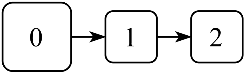
(a) Model

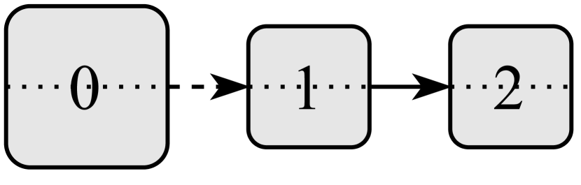
(b) MP

(c) Inter-layer-only AP

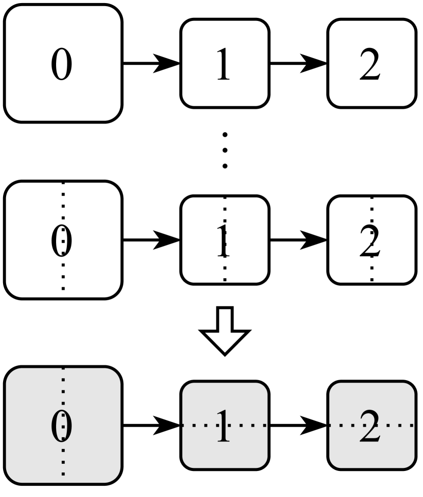
(d) Intra-layer-only AP

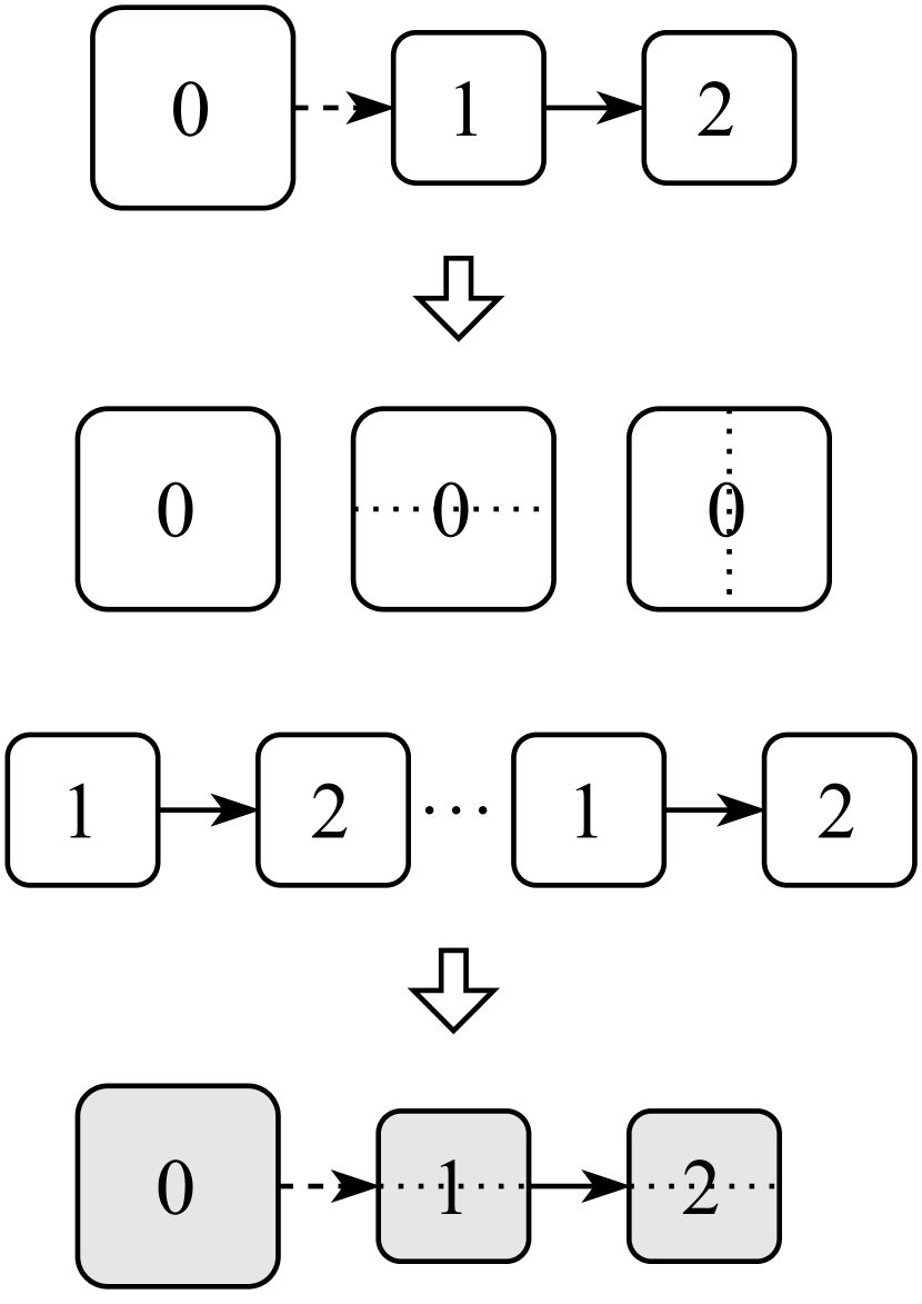
(e) Hierarchical AP

(f) UniAP

Figure 1: Parallel methods for optimizing parallel strategies for a three-layer deep learning model in (a). Numbered boxes represent the corresponding layers of the model. Layers with gray backgrounds represent the final parallel strategy for each method. Layers without dotted lines indicate that DP was applied to them, while TP was applied to the others. Solid arrows between layers represent connections within a single pipeline stage, while dashed arrows represent connections between consecutive pipeline stages.

In this section, we introduce our proposed method called UniAP. UniAP jointly optimizes the two categories of parallel strategies, including PP, DP, TP, and FSDP, to find an optimal solution. Figure 1 illustrates the difference between UniAP and other parallel methods. MP methods are manually designed with limited flexibility. Inter-layer-only and intra-layer-only AP methods optimize (search) from a set of candidate inter-layer-only and intra-layer-only parallel strategies, respectively. Hierarchical AP methods first adopt greedy or dynamic programming to propose candidate inter-layer parallel strategies. Then, they optimize the intra-layer parallel strategy for every fixed inter-layer parallel strategy. UniAP has the largest strategy space for exploration (joint optimization).

Figure 2 illustrates the flowchart of UniAP. UniAP first profiles the runtime information for the user’s hardware environment and the deep learning model. After that, UniAP estimates inter- and intra-layer costs given the computation graph and profiling results with its cost models. The estimated costs and the computation graph are then transformed into an MIQP problem. The objective function of the MIQP is to maximize the training throughput, or in other words, to minimize the time-per-iteration (TPI). By iteratively applying the cost model and MIQP with different parameters, UniAP determines the minimal TPI and its corresponding parallel strategies. We name this process the Unified Optimization Process (UOP). Finally, UniAP interprets the parallel strategies into the execution plan for the designated model.

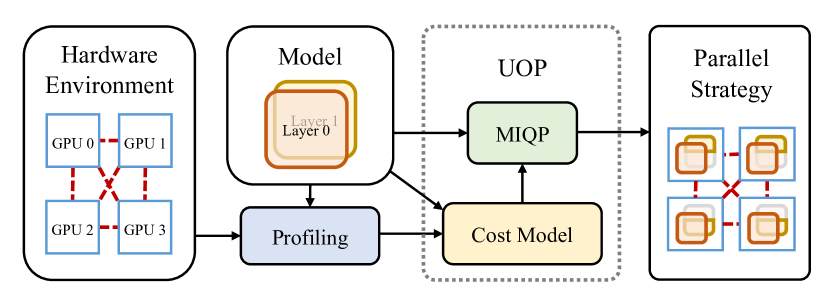
Figure 2: Flowchart of UniAP.

3.1 Profiling

UniAP collects runtime information on the hardware environment and deep learning model during profiling. For the hardware environment, UniAP evaluates the efficiency of all-reduce and point-to-point (P2P) communication for different device subsets. For example, when profiling a node with 4 GPUs, UniAP measures the all-reduce efficiency for various DP, TP, and FSDP combinations across these GPUs. Additionally, UniAP ranks these GPUs from 0 to 3 and evaluates the speed of P2P for two pipeline options: ($0\rightarrow 2$ and $1\rightarrow 3$) and ($0\rightarrow 1$, $1\rightarrow 2$ and $2\rightarrow 3$). Furthermore, UniAP estimates the computation-communication overlap coefficient (CCOC), a metric previously explored in Rashidi et al. (2021); Miao et al. (2022).

UniAP acquires two types of information for the deep learning model: computation time and memory usage. On the one hand, UniAP distinguishes the forward computation time per sample for different types of hidden layers. On the other hand, UniAP collects memory usage information for each layer, including the memory occupied by parameters and the memory usage of activation per sample in different TP sizes.

3.2 Cost Model

UniAP employs two primary cost models, namely the time cost model and the memory cost model.

Time cost model

To estimate computation time, UniAP first calculates the forward computation time by multiplying the batch size with the forward computation time per sample obtained from profiling. For Transformer-based models that mainly consist of the MatMul operator, the computation time in the BP stages is roughly twice that of the FP stages (Narayanan et al., 2021b; Li & Hoefler, 2021; Miao et al., 2022). Additionally, UniAP estimates the communication time by dividing the size of transmitting tensors by the profiled communication efficiency for different communication primitives. To accommodate overlapping, UniAP multiplies the profiled CCOC by the overlapping interval of computation and communication. To model the communication time between pipeline stages, UniAP calculates the cross-stage cost between consecutive stages by the summation of P2P costs.

Memory cost model

UniAP estimates memory consumption for each layer with its memory cost model. This estimation consists of three steps for a given layer. First, it computes the activation memory cost $m_{a}$ by multiplying the batch size and the profiled activation memory cost per sample of the TP size used by the strategy. Next, UniAP calculates the memory cost of model states $m_{s}$ for each layer based on their parameter size $ps$, TP size $ts$, FSDP size $fs$, and data type. Formally, we have

$$m_{s}=\frac{c_{dtype}\times ps}{ts\times fs},$$ (1)

where $c_{dtype}$ is a constant dependent on the data type. Finally, UniAP aggregates the activation memory cost $m_{a}$, memory cost of model states $m_{s}$, and context memory cost $m_{c}$ to a constant matrix $M$, where $M_{uk}$ denotes the memory cost for the $k$-th intra-layer strategy of layer $u$ on a single device.

3.3 Mixed Integer Quadratic Programming

The estimated costs and the computation graph are then transformed into an MIQP problem. Its formulation includes an objective function and several constraints.

3.3.1 Objective Function

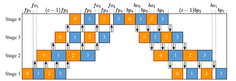
Figure 3: Time cost decomposition of a GPipe-style PP.

The objective function tries to minimize TPI. In this paper, we have chosen GPipe as our PP strategy for illustration. Figure 3 depicts the time cost decomposition of a GPipe-style PP with non-negligible communication costs. The time needed to apply gradients at the end of each iteration is not included, as it depends on the optimizer and is insignificant compared to the total time spent on FP and BP.

We denote the cost for computation stages as $\mathbb{P}=\{p_{1},p_{2},\dots,p_{deg}\}$ and the cost for communication stages as $\mathbb{O}=\{o_{1},o_{2},\dots,o_{deg-1}\}$. Here, $deg$ represents the number of computation stages, which corresponds to the degree of PP. In Figure 3, $fp_{i}$ and $bp_{i}$ denote forward and backward computation time for computation stage $i$, respectively. $fo_{j}$ and $bo_{j}$ denote forward and backward communication time for communication stage $j$, respectively. Hence, we have $p_{i}=fp_{i}+bp_{i}$ and $o_{j}=fo_{j}+bo_{j}$.

In a GPipe-style pipeline, we use $c$ to denote the number of micro-batches. As illustrated in Figure 3, a mini-batch is uniformly split into four micro-batches, and the total TPI is determined by the latency of all computation and communication stages and the latency of the slowest stage. We further denote TPI in GPipe as $tpi_{gpipe}$. Given that a stage with a higher FP computation cost leads to a higher BP computation cost with high probability, we can write the objective function of GPipe-style pipeline as follows:

$$\min tpi_{gpipe}=\sum_{i=1}^{deg}p_{i}+\sum_{j=1}^{deg-1}o_{j}+(c-1)\max\left(\mathbb{P}\cup\mathbb{O}\right).$$ (2)

3.3.2 Constraint

We first introduce additional notations before presenting the constraints. For a given layer $u\in V$, $g_{u}$ represents its set of intra-layer parallel strategies, $A_{uk}$ denotes the $k$-th intra-layer execution cost obtained from our time cost model. Additionally, we use $S_{uk}\in\{0,1\}$ to indicate whether the $k$-th parallel strategy is selected for the layer $u$, and use $P_{ui}\in\{0,1\}$ to indicate whether layer $u$ is placed on the $i$-th computation stage. Each edge $\langle u,v\rangle\in E$ is assigned a resharding cost denoted by $R_{uv}$ if the vertices are located within the same pipeline stage. Alternatively, if the vertices are located across consecutive stages, the resharding cost between them is denoted by $R^{\prime}_{uv}$. These two resharding costs are constant matrices derived from our time cost model.

Computation-stage constraint

To compute the total cost for a single computation stage $i$, all computation and communication costs associated with that stage must be aggregated and assigned to $p_{i}$. This constraint can be formulated as follows:

$$\sum_{u\in V}P_{ui}S_{u}^{\mathsf{T}}A_{u}+\sum_{\langle u,v\rangle\in E}P_{ui}P_{vi}(S_{u}^{\mathsf{T}}R_{uv}S_{v})=p_{i},$$ (3)

$$\forall i\in\{1,\dots,deg\}.$$

On the left side of (3), the first polynomial term represents the cost of choosing specific intra-layer strategies for layers placed in stage $i$. The second term represents total resharding costs within stage $i$.

Communication-stage constraint

To calculate the total cost for a single communication stage $j$, we should aggregate the P2P costs incurred between consecutive stages and assign them to $o_{j}$. This constraint can be formulated as follows:

$$\sum_{\langle u,v\rangle\in E}P_{uj}P_{v(j+1)}(S_{u}^{\mathsf{T}}R^{\prime}_{uv}S_{v}) =o_{j},$$ (4)

$$\forall j \in\{1,\dots,deg-1\}.$$

Memory constraint

We need to guarantee that no devices (GPUs) will encounter out-of-memory (OOM) exceptions during training process. This constraint can be formulated as follows:

$$\sum_{u\in V}P_{ui}S_{u}^{\mathsf{T}}M_{u}\leqslant m,~{}\forall i\in\{1,\dots,deg\}.$$ (5)

Here, $m$ denotes the memory limit for each device. In the case of homogeneous computing devices, the value of $m$ remains constant throughout all stages. But the value of $m$ varies in the case of heterogeneous computing devices.

Order-preserving constraint

PP is not a single-program multiple-data (SPMD) parallel strategy (Huang et al., 2019). Hence, we need an order-preserving constraint to ensure that the subgraphs of $\mathcal{G}$ are contiguous. We adopt the definition of contiguous from Tarnawski et al. (2020; 2021).

Definition 3.1.

A set $S\subseteq V$ is contiguous if there do not exist nodes $u\in S$, $v\in V\setminus S$, and $w\in S$ such that $v$ is reachable from $u$ and $w$ is reachable from $v$.

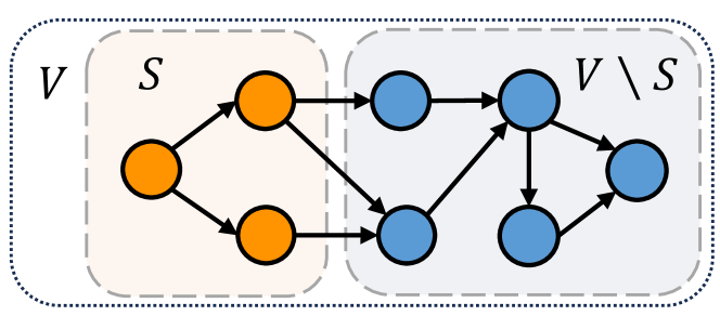
Figure 4: A contiguous set $S$.

Figure 4 illustrates an example of a contiguous set $S$, in which we cannot find any reachable node pairs $\langle u,v\rangle$ and $\langle v,w\rangle$ where $u,w\in S$ and $v\in V\setminus S$.

In our case, our model will not be assigned to different pipeline stages in a disordered manner if we ensure that all subgraphs on each computation stage are contiguous. After reformulating this constraint in linear form, we have

$$Z_{vi} \geqslant P_{vi},~{}\forall v\in V,~{}\forall i\in\{1,2,\dots,deg\},$$ (6a)

$$Z_{vi} \leqslant Z_{ui},$$

$$~{}\forall u,v\in V,~{}\forall\langle u,v\rangle\in E,~{}\forall i\in\{1,2,\dots,deg\},$$ (6b)

$$Z_{vi} \leqslant P_{vi}-P_{ui}+1,$$

$$~{}\forall u,v\in V,~{}\forall\langle u,v\rangle\in E,~{}\forall i\in\{1,2,\dots,deg\}.$$ (6c)

Detailed proof can be found in Appendix A of the supplementary material.

Layer-placement constraint

All layers should be placed on exactly one pipeline stage and at least one layer should be placed on each pipeline stage. This constraint can be formulated as follows:

$$\sum_{i=1}^{deg}P_{ui}=1, \forall u\in V,$$ (7a)

$$\sum_{u\in V}P_{ui}\geqslant 1, \forall i\in\{1,\dots,deg\},$$ (7b)

$$P_{ui}\in\{0,1\}, \forall u\in V,~{}i\in\{1,\dots,deg\}.$$ (7c)

Strategy-selection constraint

Each layer must and can choose only one strategy. This constraint can be formulated as follows:

$$\sum_{k=1}^{\lvert g_{u}\rvert}S_{uk}=1, \forall u\in V,$$ (8a)

$$S_{uk}\in\{0,1\}, \forall u\in V,~{}k\in\{1,\dots,|g_{u}|\}.$$ (8b)

The MIQP formulation for UniAP includes the objective function in (2) and all the constraints from (3) - (8b).

3.4 Unified Optimization Process

UOP integrates the cost model and MIQP based on the profiling results and the computation graph to return the optimal parallel strategy and the corresponding TPI.

First, UOP adopts intra-layer-only parallelism for initialization. Several works (Zheng et al., 2022; Liu et al., 2023) have used quadratic integer programming (QIP) to optimize intra-layer-only parallel strategy and achieved promising results. UniAP provides a QIP formulation for intra-layer-only parallelism in Appendix B of the supplementary material.

Then, UOP enumerates the pipeline degree $deg$ for the PP strategy from 2 to $n$ exponentially. For each $deg$, UOP enumerates the number of micro-batches from 2 to mini-batch size one by one and selects those divisible by the mini-batch size to ensure load balancing across micro-batches. Here, we assume the number of devices is a power of 2, and these devices are homogeneous.

For each candidate pipeline degree $deg$ and the number of micro-batches $c$, UOP formulates the cost for a training iteration to an MIQP expression. It then waits for the MIQP solver to return the optimal cost and parallel strategy under the current configuration. Specifically, our implementation adopts the Gurobi Optimizer (Gurobi Optimization, LLC, 2023) as our QIP and MIQP solver.

Finally, UOP returns the minimum cost $cost_{min}$ and its corresponding pipeline degree $deg_{min}$, number of micro-batches $c_{min}$, layer placement $P_{min}$, and intra-layer strategies $S_{min}$. We provide visualization for a candidate solution to UOP in Appendix C of the supplementary material.

Algorithm 1 Unified Optimization Process

  Input: Profiling results $PR$, strategy dictionary $SD$, mini-batch size $B$, computation graph $\mathcal{G}$, and the number of GPUs $n$.

  Output: Optimal cost $cost_{min}$, pipeline degree $deg_{min}$, the number of micro-batches $c_{min}$, layer placement $P_{min}$, and intra-layer strategy $S_{min}$

  $deg_{min}=1$;

  $c_{min}=B$;

  $A$, $R$, _, $M$ = CalculateCost($PR$, $SD[1]$, $\mathcal{G}$, $B$);

  $cost_{min}$, $P_{min}$, $S_{min}$ = QIP($A$, $R$, $M$);

  for $deg$ in {2, 4, $\dots$, $n$} do

     for $c=2$ to $B$ and $c\mid B$ do

        Micro-batch size $b=B/c$;

        $A$, $R$, $R^{\prime}$, $M$ = CalculateCost($PR$, $SD[deg]$, $\mathcal{G}$, $b$);

        $cost$, $P$, $S$ = MIQP($A$, $R$, $R^{\prime}$, $M$, $deg$, $c$);

        if $cost<cost_{min}$ then

           $cost_{min}$, $deg_{min}$, $c_{min}$, $P_{min}$, $S_{min}$ = $cost$, $deg$, $c$, $P$, $S$;

        end if

     end for

  end for

Algorithm 1 summarizes the whole process of UOP. In Algorithm 1, we denote intra-layer cost as $A$, inter-layer cost as $R$, cross-stage cost as $R^{\prime}$, and memory cost as $M$. The CalculateCost process calculates these four costs based on the cost model described in Section 3.2.

3.5 Complexity Analysis

Let $\lvert V\rvert$, $\lvert g\rvert$, and $n$ denote the number of layers, parallel strategies, and GPUs, respectively. As illustrated in Algorithm 1, UniAP exponentially enumerates all possible pipeline stages until $n$ is reached. Given a hyperparameter of mini-batch size $B$, UniAP calls CalculateCost to model the cost of each stage for each parallel strategy. Furthermore, the optimization time limit of the MIQP solver can be set as a constant hyperparameter when UniAP calls it. Therefore, the overall computational complexity of UniAP is $\mathcal{O}(\lvert V\rvert\lvert g\rvert\log(n))$.

4 Experiment

We conduct experiments on four different kinds of environments. EnvA refers to a node (machine) with 1 Xeon 6248 CPU, 8 V100-SXM2 32GB GPUs, and 472GB memory. EnvB refers to two nodes interconnected with 10Gbps networks, where each node has 2 Xeon E5-2620 v4 CPUs, 4 TITAN Xp 12GB GPUs, and 125GB memory. EnvC refers to a node with 8 A100 40GB PCIe GPUs. EnvD has four nodes, each with the same configuration as that in EnvB.

Table 1: Summary of the evaluated models. PT: Pretraining; CG: Conditional Generation; IC: Image Classification; CLM: Causal Language Modeling.

Model	Task	#params	Precision
BERT-Huge	PT	672M	FP32
T5-Large	CG	502M	FP32
ViT-Huge	IC	632M	FP32
Swin-Huge	IC	1.02B	FP32
LLaMA-7B	CLM	7B	FP16

We evaluate UniAP with five Transformer-based models, BERT-Huge (Devlin et al., 2019), T5-Large (Raffel et al., 2020), ViT-Huge (Dosovitskiy et al., 2021), Swin-Huge (Liu et al., 2021), and LLaMA (Touvron et al., 2023a; b). We follow the common practice of training these transformer-based models. To eliminate factors that affect training throughput, we turn off techniques orthogonal to parallel strategies, such as activation checkpointing (Chen et al., 2016). However, we integrate FP16 mixed precision training (Micikevicius et al., 2018) for the largest model, LLaMA, to successfully orchestrate the process. Table 1 summarizes these models.

The experimental evaluation concentrates on two primary metrics: training throughput and strategy optimization time. The former is calculated by averaging throughput from the 10th to the 60th iteration of training, while the latter is determined by measuring the time of the UOP. More details are provided in Appendix D of the supplementary material.

Table 2: Training throughput and strategy optimization time on five Transformer-based models. The number following the model’s name represents the number of hidden layers in the corresponding model. MEM$\times$ indicates out-of-memory (OOM) exceptions during strategy optimization, and CUDA$\times$ indicates CUDA OOM exceptions during model training. Due to the absence of an official JAX implementation for Swin-Huge and LLaMA in HuggingFace Transformers (v4.29), experiments involving these two models for Alpa have been excluded and denoted as N/A. The minimum and maximum training throughput speedups are calculated by dividing the average throughput of UniAP by the maximum and minimum average throughput of Galvatron and Alpa, respectively. Similarly, the minimum and maximum strategy optimization time speedup is calculated by dividing Galvatron and Alpa’s minimum and maximum average optimization time by the average optimization time of UniAP, respectively.

Env.	Model	Training Throughput (samples/s)			Minimum Speedup	Maximum Speedup
		Galvatron	Alpa	UniAP
EnvA	BERT-Huge-32	33.46 $\pm$ 0.28	31.56 $\pm$ 0.04	33.46 $\pm$ 0.28	1.00	1.06
	T5-Large-48	23.29 $\pm$ 0.04	MEM$\times$	23.29 $\pm$ 0.04	1.00	1.00
	ViT-Huge-32	109.51 $\pm$ 0.07	97.66 $\pm$ 1.42	109.51 $\pm$ 0.07	1.00	1.12
	Swin-Huge-48	CUDA$\times$	N/A	67.96 $\pm$ 0.12	N/A	N/A
EnvB	BERT-Huge-32	6.27 $\pm$ 0.17	8.95 $\pm$ 0.06	10.77 $\pm$ 0.13	1.20	1.71
	T5-Large-32	8.06 $\pm$ 0.06	MEM$\times$	7.98 $\pm$ 0.05	0.99	0.99
	ViT-Huge-32	32.20 $\pm$ 0.17	38.74 $\pm$ 0.20	45.58 $\pm$ 0.54	1.18	1.41
	Swin-Huge-48	13.90 $\pm$ 0.17	N/A	19.08 $\pm$ 0.10	1.37	1.37
EnvC	LLaMA-7B-32	1.22 $\pm$ 0.01	N/A	1.96 $\pm$ 0.03	1.61	1.61
Env.	Model	Strategy Optimization Time (min.)			Minimum Speedup	Maximum Speedup
		Galvatron	Alpa	UniAP
EnvA	BERT-Huge-32	6.44 $\pm$ 0.588	$>$ 40	0.37 $\pm$ 0.002	17.29	$>$ 107.41
	T5-Large-48	12.41 $\pm$ 0.122	MEM$\times$	0.89 $\pm$ 0.007	13.98	13.98
	ViT-Huge-32	6.29 $\pm$ 0.464	$>$ 40	0.57 $\pm$ 0.009	10.95	$>$ 69.60
	Swin-Huge-48	11.88 $\pm$ 0.666	N/A	2.16 $\pm$ 0.004	5.49	5.49
EnvB	BERT-Huge-32	2.04 $\pm$ 0.010	$>$ 40	1.51 $\pm$ 0.005	1.34	$>$ 26.32
	T5-Large-32	2.64 $\pm$ 0.110	MEM$\times$	0.91 $\pm$ 0.005	2.90	2.90
	ViT-Huge-32	2.37 $\pm$ 0.180	$>$ 40	1.11 $\pm$ 0.011	2.14	$>$ 36.01
	Swin-Huge-48	4.29 $\pm$ 0.320	N/A	2.29 $\pm$ 0.010	1.87	1.87
EnvC	LLaMA-7B-32	6.84 $\pm$ 0.055	N/A	0.49 $\pm$ 0.007	14.0	14.0

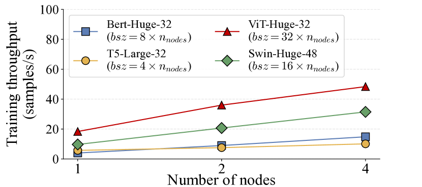
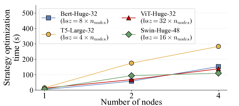
Figure 5: Training throughput and strategy optimization time with different number of nodes for different models. $n_{nodes}$ denotes the number of nodes (machines) and $bsz$ denotes the mini-batch size. Left: Training throughput. Right: Strategy optimization time.

4.1 Training Throughput and Strategy Optimization Time

We compare the training throughput and strategy optimization time of UniAP with those of the baselines on EnvA, EnvB, and EnvC. We choose Galvatron (Miao et al., 2022) and Alpa (Zheng et al., 2022) as baselines because they have achieved SOTA performance. Specifically, Galvatron has surpassed other methods, including PyTorch DDP (Li et al., 2020), Megatron-LM (Narayanan et al., 2021b), FSDP (Rajbhandari et al., 2020; FairScale authors, 2021), GPipe (Huang et al., 2019), and DeepSpeed 3D (Microsoft, 2021) in terms of training throughput, as reported in the original paper (Miao et al., 2022). Furthermore, Alpa utilizes the Just-In-Time (JIT) compilation feature in JAX and outperforms Megatron-LM and DeepSpeed.

For experiments conducted on EnvA, we set the mini-batch size to be 32, 16, 128, and 128 for BERT, T5, ViT, and Swin, respectively. For experiments conducted on EnvB, we set the mini-batch size to be 16, 8, 64, and 32 for these four models, respectively. For the LLaMA model (Touvron et al., 2023a; b) run on EnvC, we set the mini-batch size to be 8.

Table 2 shows the training throughput and strategy optimization time on EnvA, EnvB, and EnvC. On EnvA, UniAP and Galvatron get the same optimal strategy for BERT-Huge-32, T5-Large-48, and ViT-Huge-32, outperforming Alpa in terms of training throughput and strategy optimization time. In addition, UniAP finds a solution for Swin-Huge-48, while Galvatron encounters CUDA OOM problems. In particular, UniAP achieves a maximum optimization speedup that is 17$\times$ faster than Galvatron and hundreds of times faster than Alpa on BERT-Huge-32. This is mainly due to the ability of the MIQP solver to search for an optimal strategy on multiple threads, while the dynamic programming based methods like Galvatron and Alpa run on a single thread due to their strong data dependency.

On EnvB, UniAP consistently demonstrates competitive or larger training throughput compared to Galvatron and Alpa. We attribute the performance improvement to the larger strategy space in UniAP. A detailed study of the importance of strategy space is provided in Section 4.4. Furthermore, the strategy optimization time of UniAP is also significantly shorter than the two baseline methods.

For LLaMA, UniAP shows an optimization speedup of 14.0$\times$ and a training speedup of 1.61$\times$, compared to Galvatron, on EnvC.

Moreover, we find that UniAP identifies superior solutions with higher model FLOPs utilization (MFU) (Chowdhery et al., 2023), compared to Galvatron and Alpa. For example, the resulting MFUs for UniAP, Galvatron, and Alpa are 58.44%, 58.44%, and 55.10% on EnvA, while 23.6%, 13.7%, and 19.6% on EnvB. These results are due to the larger strategy space of UniAP, which is achieved by jointly optimizing inter- and intra-layer AP using an MIQP formulation. We provide a detailed case study of the optimal parallel strategy for BERT-Huge in Appendix E of the supplementary material.

4.2 Scalability

We study the scalability of UniAP on EnvD, the result of which is shown in Figure 5. We can find that the training throughput of the optimal strategy and the corresponding strategy optimization time demonstrate near-linearity as the number of nodes and mini-batch size increase. This phenomenon reveals that UniAP is scalable and verifies the computational complexity analysis in Section 3.4.

4.3 Estimation Accuracy

Some variables in UniAP and other AP methods are estimated values rather than actual running values. The TPI (inverse of training throughput) returned by UniAP and other AP methods is one of them. Accurate estimation for TPI or training throughput is crucial for evaluating candidate parallel strategies and ensuring the optimality of the solution. To quantify the accuracy of the estimated training throughput, we introduce a metric called relative estimation error (REE) $e$ for training throughput:

$$e(T,\hat{T})=\frac{|T-\hat{T}|}{T}\times 100\%,$$ (9)

where $T$ is the actual training throughput and $\hat{T}$ is the estimated training throughput.

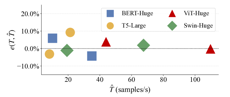
Figure 6: Relative estimation error.

We evaluate the optimal parallel strategies obtained from EnvA and EnvB and visualize the REE of UniAP in Figure 6. The results show that UniAP achieves an average REE of 3.59%, which is relatively small. In contrast, the average REE for Galvatron (Miao et al., 2022) in our experiments is 11.17%, which is larger than that of UniAP.

4.4 Ablation Study

We investigate the importance of the strategy space for the optimality of parallel strategies with an ablation study. Specifically, we constrain the strategy space to inter-layer-only and intra-layer-only strategies and evaluate the training throughput of the resulting optimal strategy on EnvB. We set the mini-batch sizes to be 16, 12, 64, and 32, respectively. The results are shown in Figure 7. We can find that constraining the strategy space compromises the optimality of parallel strategies or gets strategies that encounter OOM across different models. Hence, unifying inter- and intra-layer AP for joint optimization is essential and necessary.

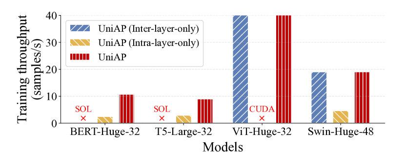
Figure 7: Ablation study. SOL$\times$ indicates no feasible solution during strategy optimization, and CUDA$\times$ indicates CUDA OOM exceptions during training.

5 Conclusion

In this paper, we propose a novel AP method called UniAP to unify inter- and intra-layer AP by MIQP. To the best of our knowledge, UniAP is the first parallel method that can jointly optimize the two categories of parallel strategies to find an optimal solution. Experimental results show that UniAP can outperform other state-of-the-art baselines to achieve the best performance.

Impact Statement

This paper proposes UniAP to advance the field of deep learning infrastructure. We have not found immediate ethical concerns or negative societal consequences of our work. Therefore, none of the negative consequences must be specifically highlighted.

However, training a Transformer-based model often requires a significant amount of energy. UniAP depicts the opportunity to greatly accelerate the training process, thereby minimizing energy consumption as much as possible. Hence, we feel the necessity to highlight its positive environmental impact here.

Appendix A Proof of the Linear Form for the Contiguous Set

To facilitate our discussion, we adopt the linear form of the order-preserving constraint as presented in the main paper. We denote $P_{ui}$ as a 0-1 variable indicating whether layer $u$ is to be placed on the $i$-th computation stage, $deg$ as the number of computation stages in the pipeline. Besides, $\mathcal{G}(V,E)$ represents the computation graph for the model. Then, we formalize the theorem as follows:

Theorem A.1.

A subgraph $V_{i}=\{\forall u\in V:P_{ui}=1\}$ is contiguous if and only if there exists $Z_{vi}$ such that (6a), (6b), and (6c) are satisfied.

Previous work (Tarnawski et al., 2020) has proven this theorem. Our proof draws on the process of this work. The details of the proof are as follows:

Proof.

”If”: Assume that there exists nodes $u,w\in V_{i}$ and $v\notin V_{i}$ such that $v$ and $w$ are reachable from $u$ and $v$, respectively. Hence, $P_{ui}=1$, $P_{wi}=1$, and $P_{vi}=0$. Without losing generality, we assume $\langle u,v\rangle\in E$. Thus, according to (6c), we have $Z_{vi}\leqslant P_{vi}-P_{ui}+1=0$. By applying (6b) repeatedly following the path from $v$ to $w$, we have $Z_{wi}\leqslant Z_{vi}$. Thus, $Z_{wi}\leqslant 0$. However, we also have $Z_{wi}\geqslant P_{wi}=1$ according to (6a). A contradiction.

”Only if”: First, we define $Z_{vi}=1$ if a node $w\in S$ is reachable from $v$. Otherwise, $Z_{vi}=0$. Thus, (6a) and (6b) are satisfied according to this kind of definition. For (6c), if $P_{vi}=1$, the constraint will hold true regardless of whether $P_{ui}$ is $1$ or $0$. If $P_{vi}=0$ and $P_{ui}=0$, $Z_{vi}\leqslant P_{vi}-P_{ui}+1=1$ will also hold true because $Z_{vi}$ could be either $0$ or $1$. Finally, if $P_{vi}=0$ and $P_{ui}=1$, $Z_{vi}=0$ will hold true because $V_{i}$ is a contiguous set and we cannot find any $w\in V_{i}$, such that $w$ is reachable from $v$. ∎

Appendix B QIP Formulation for Intra-layer-only Parallelism

Here we present the QIP formulation for intra-layer-only parallelism with explanations.

Objective function

In terms of intra-layer-only parallelism, there is only one computation stage involved. As a result, the objective function takes into account only the value of $p_{1}$. We hereby formalize the equation as

$$\min\quad tpi_{gpipe}=p_{1}.$$ (10)

Computation-stage constraint

With only one computation stage in intra-layer-only parallelism, the communication-stage constraint can be omitted, and the computation and communication cost can be modeled for $p_{1}$. Thus, we could formalize the constraint as

$$\sum_{u\in V}S_{u}^{\mathsf{T}}A_{u}+\sum_{\langle u,v\rangle\in E}S_{u}^{\mathsf{T}}R_{uv}S_{v}=p_{1}.~{}$$ (11)

In the equation, the first summation term for any $u\in V$ represents the cost of choosing intra-layer strategies for all layers, while the second term represents the summation of resharding costs on all edges.

Memory constraint

Similar to the memory constraint in MIQP, it is necessary to ensure that the memory usage on a single device does not exceed its device memory bound $m$ in QIP. This restriction gives

$$\sum_{u\in V}S_{u}^{\mathsf{T}}M_{u}\leqslant m.~{}$$ (12)

It is worth noting that $m$ should be an identical constant across multiple devices if these devices are homogeneous. Otherwise, the value of $m$ varies.

Strategy-selection constraint

For intra-layer-only parallelism, the layer-placement constraint can be safely omitted because it is designed for PP. However, the strategy-selection constraint is necessary because each layer can only select one intra-layer strategy. Therefore, the strategy-selection constraint for QIP is identical to (8a) and (8b) for MIQP.

By combining objective function (10) and constraints (8a), (8b), (11), and (12), we have the QIP expression for optimizing the intra-layer-only AP. Like MIQP expression for optimizing the inter- and intra-layer AP, UniAP will eventually get the minimum TPI and corresponding parallel strategies by invoking the off-the-shelf solver.

Appendix C Visualization for the Candidate Solution

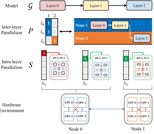
Figure 8: A candidate solution for UOP.

In this section, we proceed to visually represent a potential solution for UOP. Given a deep learning model $\mathcal{G}$, pipeline degree $deg$, and number of micro-batches $c$, UniAP will determine layer placement $P$ for inter-layer parallelism and parallel strategy $S$ for intra-layer parallelism using an off-the-shelf solver. As Figure 8 shows, the solver is optimizing a three-layer model with two pipeline stages, each assigned four GPUs. At this time, a candidate solution could be

$$P=\begin{bmatrix}1&0\\ 1&0\\ 0&1\end{bmatrix},~{}S=\begin{bmatrix}1&0&0\\ 0&1&1\\ 0&0&0\\ \vdots&\vdots&\vdots\\ 0&0&0\end{bmatrix}.$$ (13)

Here, the $u$-th row of matrix $P$ denotes the placement strategy for layer $u$, where $P_{ui}=1$ signifies the placement of layer $u$ on stage $i$, while $0$ indicates otherwise. For example, $P_{l_{0}}=\left[1,~{}0\right]$ denotes the placement of layer $l_{0}$ on pipeline stage 1. Additionally, the $u$-th column of matrix $S$ denotes the selected intra-layer parallel strategy for layer $u$, where $S_{uj}=1$ denotes the selection of the $j$-th strategy from the intra-layer parallel strategy set. For example, $S_{l_{0}}=\left[1,~{}0,~{}0,~{}\cdots,~{}0\right]^{\mathsf{T}}$ indicates that layer $l_{0}$ will adopt only the DP strategy, while $S_{l_{1}}=\left[0,~{}1,~{}0,~{}\cdots,~{}0\right]^{\mathsf{T}}$ indicates that layer $l_{1}$ will employ a strategy where DP is performed on GPU 0, 1 and GPU 2, 3, and TP is performed across these two GPU groups.

There exist numerous combinations of $P$ and $S$. The off-the-shelf solver will automatically search for the optimal solution given pipeline degree $deg$ and the number of micro-batches $c$. By solving the MIQP expression and enumerating every possible $deg$ and $c$ in the UOP process, UniAP will ultimately derive an optimal parallel strategy for the deep learning model within the current hardware environment.

Appendix D Experiment Detail

Gurobi configuration

When tackling the MIQP problem, UniAP employs several configurations for the Gurobi Optimizer 10.1 (Gurobi Optimization, LLC, 2023). In particular, we set TimeLimit to 60 seconds, MIPFocus to 1, NumericFocus to 1, and remain other configurations to default. For instance, we establish the MIPGap parameter as the default value of 1e-4 to serve as a strict termination criterion. Furthermore, we have implemented an early stopping mechanism to terminate the optimization process as early as possible. There are two conditions that can activate the mechanism. Firstly, if the current runtime exceeds 15 seconds and the relative MIP optimality gap is less than 4%, we will terminate the optimization. Secondly, if the current runtime exceeds 5 seconds and the best objective bound is worse than the optimal solution obtained in the previous optimization process, we will terminate the optimization.

Table 3: Details for five Transformer-based models. L: Number of hidden layers; H: Hidden size; S: Sequence length.

Model	L	H	S	#params
BERT-Huge	32	1280	512	672M
T5-Large	16/16	1024	512	502M
ViT-Huge	32	1280	196	632M
Swin-Huge	2/2/42/2	320/640/1280/2560	49*64/49*16/49*4/49*1	1.02B
LLaMA-7B	32	4096	2048	7B

Model detail

Table 3 presents the details of five Transformer-based models selected for our evaluations. Three of these models, namely BERT-Huge (Devlin et al., 2019), T5-Large (Raffel et al., 2020), and LLaMA-7B (Touvron et al., 2023a; b), belong to the domain of natural language processing (NLP). At the same time, the remaining two, ViT-Huge (Dosovitskiy et al., 2021) and Swin-Huge (Liu et al., 2021), are associated with computer vision (CV). It is noteworthy that BERT, ViT, and LLaMA maintain consistent types of hidden layers respectively, whereas T5 and Swin have different types of hidden layers. Numbers separated by slashes represent the statistical information for different layer types. For instance, Swin-Huge comprises four types of layers, each with 2, 2, 42, and 2 layers, respectively.

Training detail

UniAP is based on the PyTorch framework and integrates models from HuggingFace Transformers. It employs various types of parallelism, including Pipeline Parallelism (PP), Data Parallelism (DP), Tensor Parallelism (TP), and Fully Sharded Data Parallelism (FSDP), utilizing GPipe (Huang et al., 2019), PyTorch DDP (Li et al., 2020), Megatron-LM (Narayanan et al., 2021b), and FairScale (FairScale authors, 2021), respectively. For NLP models, we use the English Wikipedia dataset (Wikimedia Foundation, 2023), while the ImageNet-1K dataset (Russakovsky et al., 2015) is used for CV models. We train these models using the Adam optimizer (Kingma & Ba, 2015) and precision of FP32. We omit hyperparameters here such as learning rate and weight decay as these have minimal impact on training throughput. The model parameters in the HuggingFace Transformer are configured to align with the specifications of each individual model. For instance, we set hidden_size to 1280, num_hidden_layers to 32, num_attention_heads to 16, and seq_length to 512 for BERT-Huge. Regarding other hyperparameters in the HuggingFace configurations, we set hidden_dropout_prob and attention_probs_dropout_prob to 0.0 for ViT-Huge. For Swin-Huge, we set drop_path_rate to 0.2. We remain other configurations to default. It should be noted that the training batch sizes for each experiment are outlined in the main paper.

Appendix E Case study: BERT-Huge

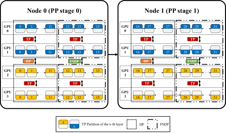
Figure 9: The optimal parallel strategy for all hidden layers of BERT-Huge on EnvB. Different colors represent different input samples in a micro-batch.

In this section, we present a visualization of the optimal parallel strategy discovered by UniAP. As represented in Figure 9, the strategy pertains to training BERT-Huge with 32 hidden layers in a 2-node environment EnvB with a mini-batch size of 16. Each node was equipped with 2 Xeon E5-2620 v4 CPUs, 4 TITAN Xp 12GB GPUs, and 125GB memory. These nodes are interconnected via a 10Gbps network. It should be noted that we only showcase the parallel strategy for the hidden layers here for simplicity but without losing generality.

Here, we provide further topological information for a node within EnvB. As illustrated in Figure 10, we categorize the GPUs numbered 0 and 1 in each node and refer to them collectively as GPUGroup0. Similarly, we label the GPUs numbered 2 and 3 as GPUGroup1. In EnvB, the interconnects within each GPU group (i.e., PCIe) have superior bandwidth than that between different groups (i.e., QPI). We collectively designate these two connection bandwidths as intra-node bandwidth, which is higher than inter-node bandwidth.

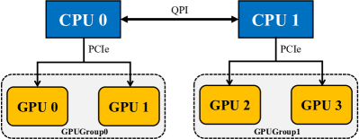
Figure 10: Topology of a node in EnvB.

In this example, UniAP has identified a parallel strategy for inter-layer parallelism that involves a two-stage pipeline. This strategy utilizes parallelism in a manner that is both efficient and effective. Specifically, the communication cost of point-to-point (P2P) between two nodes is less than that of all-reduce. Additionally, the inter-node bandwidth is lower than that of the intra-node. These factors make the two-stage PP a reasonable choice. Moreover, the pipeline has been designed such that each stage comprises an equal number of layers. This design leverages the homogeneity of the nodes and ensures load balancing across the cluster.

UniAP employs an intra-layer parallel strategy within each PP stage. It utilizes a 2-way DP for the initial 12 hidden layers in each stage between GPUGroup0 and GPUGroup1. For the remaining four hidden layers, a 2-way FSDP is utilized between GPUGroup0 and GPUGroup1 to reduce memory footprint and meet memory constraints. Within each GPU group, UniAP employs a 2-way TP for each layer. In general, TP incurs more significant communication volumes than DP and FSDP. In order to achieve maximum training throughput on EnvB, it is necessary to implement parallel strategies that prioritize higher communication volumes within each group and lower volumes between groups. Therefore, the strategy for BERT-Huge with 32 hidden layers combines the best elements of PP, DP, TP, and FSDP to maximize training throughput.

In addition, we have conducted calculations for the model FLOPs utilizatio (MFU) for Galvatron, Alpa, and UniAP in this scenario to validate our analysis. MFU is a metric introduced by Chowdhery et al. (2023), which is independent of hardware, frameworks, or implementations. Therefore, it allows us to examine the performance of different parallel strategies solely from a strategic perspective. For BERT-Huge-32, the resulting MFUs for UniAP, Galvatron, and Alpa on EnvB are 23.6%, 13.7% and 19.6% , respectively. Therefore, we conclude that UniAP does utilize its larger strategy space to find an optimal solution, rather than a sub-optimal one.

References

- Brown et al. (2020) Brown, T. B., Mann, B., Ryder, N., Subbiah, M., Kaplan, J., Dhariwal, P., Neelakantan, A., Shyam, P., Sastry, G., Askell, A., Agarwal, S., Herbert-Voss, A., Krueger, G., Henighan, T., Child, R., Ramesh, A., Ziegler, D. M., Wu, J., Winter, C., Hesse, C., Chen, M., Sigler, E., Litwin, M., Gray, S., Chess, B., Clark, J., Berner, C., McCandlish, S., Radford, A., Sutskever, I., and Amodei, D. Language Models are Few-Shot Learners. In Advances in Neural Information Processing Systems 33, pp. 1877–1901, 2020.
- Cai et al. (2022) Cai, Z., Yan, X., Ma, K., Wu, Y., Huang, Y., Cheng, J., Su, T., and Yu, F. TensorOpt: Exploring the Tradeoffs in Distributed DNN Training With Auto-Parallelism. IEEE Transactions on Parallel and Distributed Systems, 33(8):1967–1981, 2022.
- Chen et al. (2016) Chen, T., Xu, B., Zhang, C., and Guestrin, C. Training Deep Nets with Sublinear Memory Cost. CoRR, abs/1604.06174, 2016.
- Chowdhery et al. (2023) Chowdhery, A., Narang, S., Devlin, J., Bosma, M., Mishra, G., Roberts, A., Barham, P., Chung, H. W., Sutton, C., Gehrmann, S., Schuh, P., Shi, K., Tsvyashchenko, S., Maynez, J., Rao, A., Barnes, P., Tay, Y., Shazeer, N., Prabhakaran, V., Reif, E., Du, N., Hutchinson, B., Pope, R., Bradbury, J., Austin, J., Isard, M., Gur-Ari, G., Yin, P., Duke, T., Levskaya, A., Ghemawat, S., Dev, S., Michalewski, H., Garcia, X., Misra, V., Robinson, K., Fedus, L., Zhou, D., Ippolito, D., Luan, D., Lim, H., Zoph, B., Spiridonov, A., Sepassi, R., Dohan, D., Agrawal, S., Omernick, M., Dai, A. M., Pillai, T. S., Pellat, M., Lewkowycz, A., Moreira, E., Child, R., Polozov, O., Lee, K., Zhou, Z., Wang, X., Saeta, B., Diaz, M., Firat, O., Catasta, M., Wei, J., Meier-Hellstern, K., Eck, D., Dean, J., Petrov, S., and Fiedel, N. PaLM: Scaling Language Modeling with Pathways. Journal of Machine Learning Research, 24:240:1–240:113, 2023.
- Devlin et al. (2019) Devlin, J., Chang, M.-W., Lee, K., and Toutanova, K. BERT: Pre-training of Deep Bidirectional Transformers for Language Understanding. In The North American Chapter of the Association for Computational Linguistics: Human Language Technologies, pp. 4171–4186, 2019.
- Dosovitskiy et al. (2021) Dosovitskiy, A., Beyer, L., Kolesnikov, A., Weissenborn, D., Zhai, X., Unterthiner, T., Dehghani, M., Minderer, M., Heigold, G., Gelly, S., Uszkoreit, J., and Houlsby, N. An Image is Worth 16x16 Words: Transformers for Image Recognition at Scale. In International Conference on Learning Representations 9, 2021.
- Du et al. (2022) Du, N., Huang, Y., Dai, A. M., Tong, S., Lepikhin, D., Xu, Y., Krikun, M., Zhou, Y., Yu, A. W., Firat, O., Zoph, B., Fedus, L., Bosma, M. P., Zhou, Z., Wang, T., Wang, Y. E., Webster, K., Pellat, M., Robinson, K., Meier-Hellstern, K. S., Duke, T., Dixon, L., Zhang, K., Le, Q. V., Wu, Y., Chen, Z., and Cui, C. GLaM: Efficient Scaling of Language Models with Mixture-of-Experts. In International Conference on Machine Learning, pp. 5547–5569, 2022.
- FairScale authors (2021) FairScale authors. FairScale: A general purpose modular PyTorch library for high performance and large scale training. https://github.com/facebookresearch/fairscale, 2021.
- Fan et al. (2021) Fan, S., Rong, Y., Meng, C., Cao, Z., Wang, S., Zheng, Z., Wu, C., Long, G., Yang, J., Xia, L., Diao, L., Liu, X., and Lin, W. DAPPLE: A Pipelined Data Parallel Approach for Training Large Models. In Symposium on Principles and Practice of Parallel Programming, pp. 431–445, 2021.
- Fedus et al. (2022) Fedus, W., Zoph, B., and Shazeer, N. Switch Transformers: Scaling to Trillion Parameter Models with Simple and Efficient Sparsity. The Journal of Machine Learning Research, 23(120):5232–5270, 2022.
- Flynn (1966) Flynn, M. J. Very High-speed Computing Systems. Proceedings of the IEEE, 54(12):1901–1909, 1966.
- Flynn (1972) Flynn, M. J. Some Computer Organizations and Their Effectiveness. IEEE Transactions on Computers, C-21(9):948–960, 1972.
- Gurobi Optimization, LLC (2023) Gurobi Optimization, LLC. Gurobi Optimizer Reference Manual. https://www.gurobi.com, 2023.
- He et al. (2021) He, C., Li, S., Soltanolkotabi, M., and Avestimehr, S. PipeTransformer: Automated Elastic Pipelining for Distributed Training of Large-scale Models. In International Conference on Machine Learning, pp. 4150–4159, 2021.
- Huang et al. (2019) Huang, Y., Cheng, Y., Bapna, A., Firat, O., Chen, D., Chen, M. X., Lee, H., Ngiam, J., Le, Q. V., Wu, Y., and Chen, Z. GPipe: Efficient Training of Giant Neural Networks using Pipeline Parallelism. In Advances in Neural Information Processing Systems 32, pp. 103–112, 2019.
- Jia et al. (2018) Jia, Z., Lin, S., Qi, C. R., and Aiken, A. Exploring Hidden Dimensions in Parallelizing Convolutional Neural Networks. In International Conference on Machine Learning, pp. 2279–2288, 2018.
- Jia et al. (2019) Jia, Z., Zaharia, M., and Aiken, A. Beyond Data and Model Parallelism for Deep Neural Networks. In Machine Learning and Systems, pp. 1–13, 2019.
- Kingma & Ba (2015) Kingma, D. P. and Ba, J. Adam: A Method for Stochastic Optimization. In 3rd International Conference on Learning Representations, 2015.
- Lazimy (1982) Lazimy, R. Mixed-integer Quadratic Programming. Math. Program., 22(1):332–349, December 1982.
- Lepikhin et al. (2021) Lepikhin, D., Lee, H., Xu, Y., Chen, D., Firat, O., Huang, Y., Krikun, M., Shazeer, N., and Chen, Z. GShard: Scaling Giant Models with Conditional Computation and Automatic Sharding. In International Conference on Learning Representations, 2021.
- Li & Hoefler (2021) Li, S. and Hoefler, T. Chimera: Efficiently Training Large-Scale Neural Networks with Bidirectional Pipelines. In International Conference for High Performance Computing, Networking, Storage and Analysis, pp. 27:1–27:14, 2021.
- Li et al. (2020) Li, S., Zhao, Y., Varma, R., Salpekar, O., Noordhuis, P., Li, T., Paszke, A., Smith, J., Vaughan, B., Damania, P., and Chintala, S. PyTorch Distributed: Experiences on Accelerating Data Parallel Training. Proceedings of the VLDB Endowment, 13(12):3005–3018, 2020.
- Liu et al. (2023) Liu, Y., Li, S., Fang, J., Shao, Y., Yao, B., and You, Y. Colossal-Auto: Unified Automation of Parallelization and Activation Checkpoint for Large-scale Models. CoRR, abs/2302.02599, 2023.
- Liu et al. (2021) Liu, Z., Lin, Y., Cao, Y., Hu, H., Wei, Y., Zhang, Z., Lin, S., and Guo, B. Swin Transformer: Hierarchical Vision Transformer using Shifted Windows. In International Conference on Computer Vision, pp. 9992–10002, 2021.
- Miao et al. (2022) Miao, X., Wang, Y., Jiang, Y., Shi, C., Nie, X., Zhang, H., and Cui, B. Galvatron: Efficient Transformer Training over Multiple GPUs Using Automatic Parallelism. Proceedings of the VLDB Endowment, 16(3):470–479, 2022.
- Micikevicius et al. (2018) Micikevicius, P., Narang, S., Alben, J., Diamos, G. F., Elsen, E., García, D., Ginsburg, B., Houston, M., Kuchaiev, O., Venkatesh, G., and Wu, H. Mixed Precision Training. In International Conference on Learning Representations, 2018.
- Microsoft (2021) Microsoft. Deepspeed 3D. https://github.com/microsoft/Megatron-DeepSpeed/blob/main/examples/pretrain_bert_distributed_with_mp.sh, 2021.
- Narayanan et al. (2019) Narayanan, D., Harlap, A., Phanishayee, A., Seshadri, V., Devanur, N. R., Ganger, G. R., Gibbons, P. B., and Zaharia, M. PipeDream: Generalized Pipeline Parallelism for DNN Training. In Symposium on Operating Systems Principles, pp. 1–15, 2019.
- Narayanan et al. (2021a) Narayanan, D., Phanishayee, A., Shi, K., Chen, X., and Zaharia, M. Memory-Efficient Pipeline-Parallel DNN Training. In International Conference on Machine Learning, pp. 7937–7947, 2021a.
- Narayanan et al. (2021b) Narayanan, D., Shoeybi, M., Casper, J., LeGresley, P., Patwary, M., Korthikanti, V., Vainbrand, D., Kashinkunti, P., Bernauer, J., Catanzaro, B., Phanishayee, A., and Zaharia, M. Efficient Large-scale Language Model Training on GPU Clusters Using Megatron-LM. In International Conference for High Performance Computing, Networking, Storage and Analysis, pp. 58:1–58:15, 2021b.
- Raffel et al. (2020) Raffel, C., Shazeer, N., Roberts, A., Lee, K., Narang, S., Matena, M., Zhou, Y., Li, W., and Liu, P. J. Exploring the limits of transfer learning with a unified text-to-text transformer. The Journal of Machine Learning Research, 21(1):5485–5551, 2020.
- Rajbhandari et al. (2020) Rajbhandari, S., Rasley, J., Ruwase, O., and He, Y. ZeRO: Memory Optimizations Toward Training Trillion Parameter Models. In International Conference for High Performance Computing, Networking, Storage and Analysis, pp. 20:1–20:16, 2020.
- Rashidi et al. (2021) Rashidi, S., Denton, M., Sridharan, S., Srinivasan, S., Suresh, A., Nie, J., and Krishna, T. Enabling Compute-Communication Overlap in Distributed Deep Learning Training Platforms. In International Symposium on Computer Architecture, pp. 540–553, 2021.
- Rasley et al. (2020) Rasley, J., Rajbhandari, S., Ruwase, O., and He, Y. DeepSpeed: System Optimizations Enable Training Deep Learning Models with Over 100 Billion Parameters. In The 26th ACM SIGKDD Conference on Knowledge Discovery and Data Mining, pp. 3505–3506, 2020.
- Russakovsky et al. (2015) Russakovsky, O., Deng, J., Su, H., Krause, J., Satheesh, S., Ma, S., Huang, Z., Karpathy, A., Khosla, A., Bernstein, M., Berg, A. C., and Fei-Fei, L. ImageNet Large Scale Visual Recognition Challenge. International Journal of Computer Vision, 115(3):211–252, 2015.
- Schaarschmidt et al. (2021) Schaarschmidt, M., Grewe, D., Vytiniotis, D., Paszke, A., Schmid, G. S., Norman, T., Molloy, J., Godwin, J., Rink, N. A., Nair, V., and Belov, D. Automap: Towards Ergonomic Automated Parallelism for ML Models. CoRR, abs/2112.02958, 2021.
- Shazeer et al. (2018) Shazeer, N., Cheng, Y., Parmar, N., Tran, D., Vaswani, A., Koanantakool, P., Hawkins, P., Lee, H., Hong, M., Young, C., Sepassi, R., and Hechtman, B. A. Mesh-TensorFlow: Deep Learning for Supercomputers. In Advances in Neural Information Processing Systems 31, pp. 10435–10444, 2018.
- Tarnawski et al. (2020) Tarnawski, J., Phanishayee, A., Devanur, N. R., Mahajan, D., and Paravecino, F. N. Efficient Algorithms for Device Placement of DNN Graph Operators. In Advances in Neural Information Processing Systems 33, pp. 15451–15463, 2020.
- Tarnawski et al. (2021) Tarnawski, J., Narayanan, D., and Phanishayee, A. Piper: Multidimensional Planner for DNN Parallelization. In Advances in Neural Information Processing Systems 34, pp. 24829–24840, 2021.
- Touvron et al. (2023a) Touvron, H., Lavril, T., Izacard, G., Martinet, X., Lachaux, M.-A., Lacroix, T., Rozière, B., Goyal, N., Hambro, E., Azhar, F., Rodriguez, A., Joulin, A., Grave, E., and Lample, G. LLaMA: Open and Efficient Foundation Language Models. CoRR, abs/2302.13971, 2023a.
- Touvron et al. (2023b) Touvron, H., Martin, L., Stone, K., Albert, P., Almahairi, A., Babaei, Y., Bashlykov, N., Batra, S., Bhargava, P., Bhosale, S., Bikel, D., Blecher, L., Canton-Ferrer, C., Chen, M., Cucurull, G., Esiobu, D., Fernandes, J., Fu, J., Fu, W., Fuller, B., Gao, C., Goswami, V., Goyal, N., Hartshorn, A., Hosseini, S., Hou, R., Inan, H., Kardas, M., Kerkez, V., Khabsa, M., Kloumann, I., Korenev, A., Koura, P. S., Lachaux, M.-A., Lavril, T., Lee, J., Liskovich, D., Lu, Y., Mao, Y., Martinet, X., Mihaylov, T., Mishra, P., Molybog, I., Nie, Y., Poulton, A., Reizenstein, J., Rungta, R., Saladi, K., Schelten, A., Silva, R., Smith, E. M., Subramanian, R., Tan, X. E., Tang, B., Taylor, R., Williams, A., Kuan, J. X., Xu, P., Yan, Z., Zarov, I., Zhang, Y., Fan, A., Kambadur, M., Narang, S., Rodriguez, A., Stojnic, R., Edunov, S., and Scialom, T. Llama 2: Open Foundation and Fine-Tuned Chat Models. CoRR, abs/2307.09288, 2023b.
- Wang et al. (2019) Wang, M., Huang, C.-C., and Li, J. Supporting Very Large Models using Automatic Dataflow Graph Partitioning. In Proceedings of the Fourteenth EuroSys Conference, pp. 26:1–26:17, 2019.
- Wikimedia Foundation (2023) Wikimedia Foundation. Wikimedia Downloads. https://dumps.wikimedia.org, 2023.
- Xu et al. (2021) Xu, Y., Lee, H., Chen, D., Hechtman, B. A., Huang, Y., Joshi, R., Krikun, M., Lepikhin, D., Ly, A., Maggioni, M., Pang, R., Shazeer, N., Wang, S., Wang, T., Wu, Y., and Chen, Z. GSPMD: General and Scalable Parallelization for ML Computation Graphs. CoRR, abs/2105.04663, 2021.
- Zhao et al. (2022) Zhao, S., Li, F., Chen, X., Guan, X., Jiang, J., Huang, D., Qing, Y., Wang, S., Wang, P., Zhang, G., Li, C., Luo, P., and Cui, H. vPipe: A Virtualized Acceleration System for Achieving Efficient and Scalable Pipeline Parallel DNN Training. IEEE Transactions on Parallel and Distributed Systems, 33(3):489–506, 2022.
- Zheng et al. (2022) Zheng, L., Li, Z., Zhang, H., Zhuang, Y., Chen, Z., Huang, Y., Wang, Y., Xu, Y., Zhuo, D., Xing, E. P., Gonzalez, J. E., and Stoica, I. Alpa: Automating Inter- and Intra-Operator Parallelism for Distributed Deep Learning. In USENIX Symposium on Operating Systems Design and Implementation, pp. 559–578, 2022.