Pulsar timing array observations as possible hints for nonsingular cosmology

Abstract

Recent pulsar timing array (PTA) experiments have reported strong evidence of the stochastic gravitational wave background (SGWB). If interpreted as primordial gravitational waves (GWs), the signal favors a strongly blue-tilted spectrum. Consequently, the nonsingular cosmology, which is able to predict a strongly blue-tilted GW spectrum with $n_{T}\simeq 2$ on certain scales, offers a potential explanation for the observed SGWB signal. In this paper, we present a Genesis-inflation model capable of explaining the SGWB signal observed by the PTA collaborations while also overcoming the initial singularity problem associated with the inflationary cosmology. Furthermore, our model predicts distinctive features in the SGWB spectrum, which might be examined by forthcoming space-based gravitational wave experiments.

I Introduction

Inflation is the standard paradigm of the primordial Universe, providing a natural way to explain the formation of large scale structure and the observation of cosmic microwave background (CMB). Nonetheless, it is argued that inflation suffers from the initial singularity problem Borde and Vilenkin (1994); Borde et al. (2003) (see, e.g., Lesnefsky et al. (2023); Geshnizjani et al. (2023) for recent development). Therefore, it is interesting to investigate nonsingular cosmologies, i.e. cosmological models that do not suffer the initial singularity problem, such as the bouncing cosmology Gasperini and Veneziano (1993); Finelli and Brandenberger (2002); Piao et al. (2004); Piao (2004, 2005); Cai et al. (2007, 2011); Easson et al. (2011); Cai et al. (2012); Liu et al. (2013); Qiu et al. (2013); Koehn et al. (2014); Wan et al. (2015); Qiu and Wang (2015); Nojiri et al. (2016); Banerjee and Saridakis (2017); Chen et al. (2018); Mironov et al. (2018); Akama and Kobayashi (2019); Ye and Piao (2019a); Akama et al. (2020); Ye and Piao (2019b); Mironov et al. (2020); Nandi and Sriramkumar (2020); Nandi (2021); Battista (2021); Zhu et al. (2021); Banerjee et al. (2022); Ganz et al. (2023); Zhu and Cai (2023); Singh et al. (2023); Burkmar and Bruni (2023); Kaur et al. (2023); Tripathy et al. (2023) and Genesis cosmology Creminelli et al. (2010); Liu et al. (2011); Wang and Brandenberger (2012); Liu and Piao (2013); Creminelli et al. (2013); Hinterbichler et al. (2012, 2013); Easson et al. (2013); Liu et al. (2014); Pirtskhalava et al. (2014); Nishi and Kobayashi (2015); Cai and Piao (2016); Nishi and Kobayashi (2017); Dobre et al. (2018); Mironov et al. (2019); Zhu and Zheng (2021); Cai et al. (2022) (see also Piao and Zhou (2003); Piao (2007)).

The standard slow-roll inflation predicts a nearly scale-invariant tensor spectrum with a tensor spectral index $n_{T}\simeq 0$. On the contrary, many nonsingular scenarios predict strongly blue-tilted tensor spectra with $2\lesssim n_{T}\lesssim 3$ on certain scales Khoury et al. (2001); Boyle et al. (2004); Qiu et al. (2011); Nishi and Kobayashi (2016), provided the initial state of perturbation mode is set as the Bunch-Davis vacuum. By introducing additional mechanisms during inflation, such as an intermediate null energy condition violation or a diminishment of propagating speed of Gravitational Waves (GWs), we can also obtain blue tensor spectra with $0<n_{T}\lesssim 2$ Piao and Zhang (2004a); Wang and Xue (2014); Cai et al. (2016a, b); Wang et al. (2017); Cai and Piao (2021, 2022). Therefore, the primordial gravitational wave (PGW) signal could be a promising tool for distinguishing canonical slow-roll inflation and its competitors or modifications, including certain nonsingular cosmologies.

Recently, pulsar timing array (PTA) collaborations, including NANOGrav Afzal et al. (2023); Agazie et al. (2023), EPTA Antoniadis et al. (2023a), PPTA Reardon et al. (2023), and CPTA Xu et al. (2023), have reported strong evidence for an isotropic stochastic GW background with a strain amplitude of order $\mathcal{O}(10^{-15})$ at the reference frequency $f=1\,\textnormal{yr}^{-1}$. The PTA result strongly supports a blue tensor spectrum with $n_{T}=1.8\pm 0.3$ (see e.g., Afzal et al. (2023); Antoniadis et al. (2023b); Vagnozzi (2023)). This value of $n_{T}$ still falls within the range predicted by various primordial cosmological scenarios (see Piao and Zhang (2004b) for the spectra index of various expanding and contracting phases). It is then natural to ask if it is possible to interpret the PTA signals to be originated from PGWs in nonsingular cosmology.

In the minimal setting, nonsingular cosmologies like Ekpyrotic bounce and Genesis cosmology predict blue tensor spectra on all scales, which is not realistic: the power spectrum of tensor perturbation (i.e., $P_{T}$) is either too small to be observed on the PTA scale or grows too large on smaller scales to invalidate the perturbation theory. Additionally, for a power law like $P_{T}\sim k^{n_{T}}$ in inflationary scenario, there is a very low upper limit on the reheating temperature (i.e., $T_{\mathrm{rh}}\lesssim 10$ GeV Vagnozzi (2023)) due to the constraint on the $e$-folding number of inflation implied by $P_{T}<1$. A realistic candidate for an early universe model might be a combination of nonsingular cosmology and inflation, which is able to naturally terminate the blue nature of $P_{T}$ on certain scales as well as resolve the cosmological singularity problem.

As a start, we begin with a Genesis-inflation model Cai et al. (2017a), due to its relative simplicity. We construct a specific Genesis-inflation model such that the scalar spectrum is scale-invariant in both the quasi-Minkowskian epoch and the inflation epoch, consistent with CMB observations. The tensor spectrum is blue-tilted across a broad frequency range from the observational window of CMB to that of PTA, and scale-invariant on smaller scales, with oscillatory features on a short range of scales corresponding to the transition epoch. We find that the PGW generated in this model can successfully explain the PTA data, while its tail in the higher frequency band might be accessible to future GW detectors such as LISA Amaro-Seoane et al. (2017), Taiji Hu and Wu (2017) and TianQin Luo et al. (2016).

This paper is organized as follows. In Sec. II, we introduce our toy model of Genesis-inflation. We analyze the dynamics of perturbation in Sec. III, then numerically evaluate the tensor perturbation and confront it with PTA observations in Sec. IV. We conclude in Sec. V. We take the sign of the metric as $(-,+,+,+)$ throughout. The canonical kinetic term of the scalar field $\phi$ is defined as $X\equiv-\frac{1}{2}\nabla_{\mu}\phi\nabla^{\mu}\phi$, which is simply $X=\dot{\phi}^{2}/2$ at the background level. The d’Alembert operator is $\Box\equiv\nabla_{\mu}\nabla^{\mu}$. We have also set $M_{p}\equiv(8\pi G)^{-1/2}=1$ for simplicity.

II A simple Genesis model

II.1 Action

The “no-go” theorem, as proven in Libanov et al. (2016); Kobayashi (2016), indicates that spatially flat nonsingular cosmologies constructed within Horndeski theories are plagued by ghost or gradient instabilities. However, it has been demonstrated within the framework of effective field theory (EFT) that these instabilities can be eliminated through the use of “beyond Horndeski” operators Cai et al. (2017b); Creminelli et al. (2016); Cai et al. (2017a); Cai and Piao (2017); Kolevatov et al. (2017) (see also Mironov et al. (2019); Ilyas et al. (2021); Zhu and Zheng (2021); Cai et al. (2022) for developments in Genesis cosmology). Notably, it is demonstrated in Cai et al. (2017a) with the least set of EFT operators that a fully stable nonsingular Genesis-inflation model can be implemented.

In this paper, we start with the action

$$S=\int d^{4}x\sqrt{-g}\left(\frac{R}{2}+\mathcal{L}_{H2}+\mathcal{L}_{H3}+\mathcal{L}_{\mathrm{EFT}}\right)~{},$$ (1)

where $R/2$ is the standard Einstein-Hilbert action, $\mathcal{L}_{H2}$ and $\mathcal{L}_{H3}$ are the Horndeski Lagrangian. Specifically, we take

$$\mathcal{L}_{H2}=g_{1}(\phi)X+g_{2}(\phi)X^{2}-V(\phi)~{},\quad~{}\mathcal{L}_{H3}=-\gamma X^{2}\Box\phi~{}.$$ (2)

The EFT Lagrangian $\mathcal{L}_{\mathrm{EFT}}$ in (1) represents the “beyond Horndeski” operators, which are able to stabilize the scalar perturbations. As we primarily focus on primordial GWs in this paper, we will not delve into the details of $\mathcal{L}_{\mathrm{EFT}}$, see e.g. Cai et al. (2017a).

In a spatially flat FLRW universe

$$ds^{2}=-dt^{2}+a(t)^{2}d\vec{x}^{2}~{},$$ (3)

the Friedmann equations are

$$3H^{2}=\rho_{\phi}=\frac{1}{2}g_{1}\dot{\phi}^{2}+\frac{3}{4}g_{2}\dot{\phi}^{4}+3H\gamma\dot{\phi}^{5}+V(\phi)~{},$$ (4)

$$\dot{H}=-\frac{1}{2}\left(\rho_{\phi}+p_{\phi}\right)=-\frac{1}{2}g_{1}\dot{\phi}^{2}-\frac{1}{2}g_{2}\dot{\phi}^{4}-\frac{1}{2}\gamma\dot{\phi}^{4}(3\dot{\phi}H-\ddot{\phi})~{}.$$ (5)

where $H$ is the Hubble parameter, $\rho_{\phi}$ and $p_{\phi}$ are the density and pressure of the matter field $\phi$. An overdot represents the differentiation with respect to the physical time $t$.

As we will show in Sec. II.2, a Genesis solution with a scale-invariant scalar spectrum can be realised by the following choice of auxiliary functions

$$g_{1}(\phi)=-\frac{3\kappa^{2}e^{4\phi}}{2}\frac{1-\tanh\omega_{1}(\phi-\phi_{1})}{2}~{},\quad~{}g_{2}(\phi)=e^{2\phi}\frac{1+e^{2\phi}}{1+e^{4\phi}}~{},~{}$$ (6)

$$V(\phi)=\frac{1}{2}m^{2}\left(1-\frac{\phi^{2}}{\phi_{0}^{2}}\right)^{2}\left(\frac{1+\tanh\omega_{2}(\phi-\phi_{2})}{2}\right)~{}.$$ (7)

II.2 The Genesis solution

Assuming the universe adopts a Genesis solution in the past infinity with $\phi\to-\infty$, we expect the auxiliary functions to have the following asymptotic behavior:

$$\lim_{\phi\to-\infty}g_{1}(\phi)=-\frac{3}{2}\kappa^{2}e^{4\phi}~{},~{}\lim_{\phi\to-\infty}g_{2}(\phi)=e^{2\phi}~{},~{}\lim_{\phi\to-\infty}V(\phi)=0~{}.$$ (8)

Moreover, to have a late-time slow-roll inflationary epoch, we need a flat potential:

$$\lim_{\phi\to+\infty}g_{1}(\phi)=0~{},~{}\lim_{\phi\to+\infty}g_{2}(\phi)=1~{},~{}\lim_{\phi\to+\infty}V(\phi)=\frac{1}{2}m^{2}\left(1-\frac{\phi^{2}}{\phi_{0}^{2}}\right)^{2}~{}.$$ (9)

Therefore, we choose the explicit functions (6) and (7) to smoothly connect the asymptotic forms (8) and (9).

The Friedmann equations in the far past, with the asymptotic behavior (8), gives

$$3H^{2}=-\frac{3}{4}\kappa^{2}e^{4\phi}\dot{\phi}^{2}+\frac{3}{4}e^{2\phi}\dot{\phi}^{4}+3H\gamma\dot{\phi}^{5}~{},$$ (10)

which permits a quasi-Minkowskian solution

$$\dot{\phi}^{2}e^{-2\phi}=\kappa^{2}~{}\to~{}\phi=\ln\left[\frac{1}{\kappa(-t)}\right]~{},~{}\dot{\phi}=\frac{1}{-t}~{},~{}e^{\phi}=\frac{1}{\kappa(-t)}~{}.$$ (11)

The second Friedmann equation reads

$$\dot{H}\simeq\frac{1+2\kappa^{2}\gamma}{4\kappa^{2}}\frac{1}{(-t)^{6}}~{}\to~{}H\simeq\frac{1+2\kappa^{2}\gamma}{20\kappa^{2}}\frac{1}{(-t)^{5}}>0~{}.$$ (12)

We will use (11) and (12) as the initial condition for the numerical evaluation.

II.3 Illustration of background dynamics

We numerically evaluate the background dynamics in this section. We adopt the parameter setting

$$\kappa=\frac{1}{12}~{},~{}\gamma=72~{},~{}m=0.08~{};$$ (13)

$$\omega_{1}=18~{},~{}\omega_{2}=20~{},~{}\phi_{0}=2000~{},~{}\phi_{1}=2.1~{},~{}\phi_{2}=2.6~{}.$$ (14)

The parameter set (14) ensures the asymptotic behavior (8) and (9), and has little influence on the relevant physics. We plot the auxiliary functions $g_{1}$, $g_{2}$ and $V$ in Fig. 1.

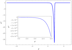
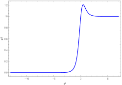
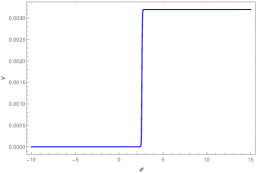
Figure 1: The auxiliary functions.

On the other hand, the parameters (13) determine the physics of Genesis cosmology. From (12) we see that $\kappa$ and $\gamma$ determine the Hubble parameter in the quasi-Minkowskian epoch. Moreover, in Sec. III.4 we will show that the sound speed of scalar perturbation $c_{s}^{2}$ in the quasi-Minkowskian epoch is also determined by $\kappa$ and $\gamma$, and we choose (13) such that $c_{s}^{2}=1$. The parameter $m$ determines the height of “cliff” in the inflationary potential $V(\phi)$, and thus the Hubble parameter in the inflation stage.

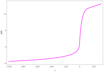
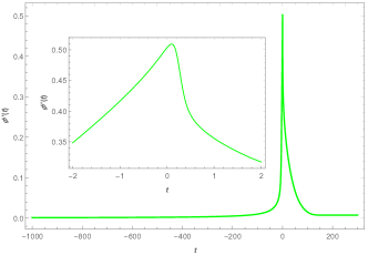
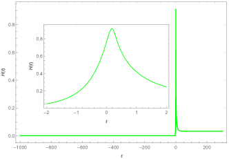
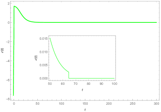
Figure 2: The background dynamics of our Genesis-inflation model with parameter setting (13), (14). The upper panel shows the dynamics of the scalar field, while the lower panel shows the dynamics of the background evolution.

We illustrate the background dynamics of our model in Fig. 2. The quasi-Minkowskian epoch is characterized by the $H\to 0$ behavior when $t<0$. After a short transition epoch around $t=0$, the universe enters an inflation epoch with a nearly constant $H$.

III Perturbation

III.1 Dynamic equation

The scalar and tensor perturbations at the quadratic level can be expressed as

$$S_{2,s}=\int d\tau d^{3}x\frac{z_{s}^{2}}{2}\left[\zeta^{\prime 2}-c_{s}^{2}(\partial_{i}\zeta)^{2}\right]~{},$$ (15)

$$S_{2,T}=\int d\tau d^{3}x\frac{a^{2}}{8}\left[\gamma_{ij}^{\prime 2}-c_{T}^{2}\gamma_{ij}^{2}\right]~{},$$ (16)

where $\zeta$ is the curvature perturbation and $\gamma_{ij}$ represents the tensor perturbation. Here for simplicity, we suppress the polarization tensor for the tensor sector. We have

$$\frac{z_{s}^{2}}{2a^{2}}=3+2\frac{\dot{\phi}^{2}(g_{1}+3g_{2}\dot{\phi}^{2})+18H\gamma\dot{\phi}^{5}-6H^{2}}{(2H-\gamma\dot{\phi}^{5})^{2}}~{},$$ (17)

and

$$\left(-\frac{z_{s}^{2}}{2a^{2}}\right)c_{s}^{2}=1-\frac{2}{a}\frac{d}{dt}\left(\frac{a}{2H-\gamma\dot{\phi}^{5}}\right)=\frac{\gamma^{2}\dot{\phi}^{10}-2\gamma H\dot{\phi}^{5}-10\gamma\dot{\phi}^{4}\ddot{\phi}+4\dot{H}}{(2H-\gamma\dot{\phi}^{5})^{2}}~{}.$$ (18)

in the quasi-Minkowskian epoch and the inflation epoch Ilyas et al. (2020).

Notably, the behavior of $c_{s}^{2}$ is dependent on the EFT action in the transition epoch. However, in our case we are interested in the scale-invariance behavior: the scale invariance in the quasi-Minkowskian epoch can be used to interpret the CMB result, while the scale invariance in the inflation epoch guarantees the scalar perturbation does not grow on small scales and invalidate the perturbation theory. Therefore, let’s simply assume that the EFT action is delicately designed, such that $c_{s}^{2}>0$ in the transition period, and no gradient instability occurs.

The dynamical equation of the scalar and tensor perturbation is

$$v_{k}^{\prime\prime}+\left(k^{2}c_{s}^{2}-\frac{z_{s}^{\prime\prime}}{z_{s}}\right)v_{k}=0~{},$$ (19)

$$\nu_{k}^{\prime\prime}+\left(c_{T}^{2}k^{2}-\frac{a^{\prime\prime}}{a}\right)\nu_{k}=0~{},$$ (20)

where $v_{k}\equiv z_{s}\zeta$ and $\nu_{k}\equiv 1/2a\gamma_{k}$ are the corresponding mode functions and a prime denotes differentiation with respect to the conformal time $d\tau=dt/a$.

III.2 Effective horizon

Since the expression $z_{s}^{2}$ in the quasi-Minkowskian epoch, (17), is non-trivial, let’s define the effective “Hubble horizon” for scalar and tensor perturbation:

$$H_{s}^{2}\equiv z_{s}^{\prime\prime}/z_{s}~{},~{}H_{T}^{2}\equiv a^{\prime\prime}/a~{}.$$ (21)

From the dynamical equations (19) and (20), we see the effective Hubble parameters determine the evolution of perturbations.

Let’s first come to the tensor mode. The effective Hubble parameter behaves as

$$\lim_{t\to-\infty}H_{T}^{2}=a^{2}(2H^{2}+\dot{H})\propto(-t)^{-6}\simeq 0~{},~{}\lim_{t\to\infty}H_{T}^{2}=a^{2}H^{2}(2-\epsilon)\simeq\frac{2}{\tau^{2}}~{}.$$ (22)

Therefore, the tensor perturbation will remain in the vacuum state in the quasi-Minkowskian epoch, and thus the tensor spectra index is simply $n_{T}=2$. In the subsequent inflationary epoch, modes crossing the effective horizon would be redshifted and get a nearly scale-invariant tensor spectrum with $n_{T}=0$, as predicted by the standard slow-roll inflation.

Denoting the minimal value of $H_{T}^{2}$ in the inflationary epoch to be $H_{T,\min}$, we can estimate

$$n_{T}=2~{},~{}k<k_{T}~{};~{}n_{T}=0~{},~{}k>k_{T}~{};~{}k_{T}\equiv H_{T,\min}~{}.$$ (23)

The behavior of $H_{S}^{2}$ is more complicated. However, as we shall elaborate in Sec. III.4, for modes crossing the effective Hubble horizon during the quasi-Minkowskian epoch and the inflationary epoch, their corresponding scalar spectra index is $n_{s}\simeq 1$. Thus, we expect the scalar spectrum to be almost scale-invariant, except for a possible feature at scales corresponding to the transition epoch.

III.3 Tensor spectra

In the quasi-Minkowskian epoch, $H_{T}^{2}$ is approximately zero, so the dynamical equation is simply

$$\mu_{k}^{\prime\prime}+k^{2}\mu_{k}=0~{}\to~{}|\mu_{k}|=\frac{1}{\sqrt{2k}}~{},$$ (24)

after imposing the vacuum initial condition. The corresponding tensor spectrum is

$$P_{T}\equiv\frac{4k^{3}}{\pi^{2}}\frac{|\mu_{k}|^{2}}{a^{2}}\simeq\frac{2}{\pi^{2}}\left(\frac{k}{a_{0}}\right)^{2}~{},$$ (25)

where $a_{0}$ represents the scale factor during the Genesis epoch, $k/a_{0}$ is the physical wavenumber. Apparently, for the modes that exit the horizon during the Genesis epoch, the tensor spectral index is $n_{T}=2$.

During the inflationary epoch, the dynamic equation takes the form

$$\mu_{k}^{\prime\prime}+\left(k^{2}-\frac{2}{(\tau-\tau_{e})^{2}}\right)\mu_{k}=0,$$ (26)

where $\tau_{e}$ is an integration constant. Denoting the start time of inflation as $\tau_{I}$, we find

$$k_{T}\equiv H_{T,\min}=\frac{\sqrt{2}}{|\tau_{I}-\tau_{e}|}~{}.$$ (27)

For modes with $k<k_{T}$, they are already superhorizon at the start of inflation, and thus their amplitude remains constant. The corresponding spectrum is described by (25), where $a=a(\tau_{M})$, with $\tau_{M}$ denoting the end of the quasi-Minkowskian state. On the other hand, for modes with $k>k_{I}$, the general solution with vacuum initial conditions is given by

$$\mu_{k}=\frac{\sqrt{{\pi}|\tau-\tau_{e}|}}{2}H_{3/2}^{(1)}(k|\tau-\tau_{e}|)=\frac{-i-k|\tau-\tau_{e}|}{\sqrt{2}k^{3/2}|\tau-\tau_{e}|}e^{ik|\tau-\tau_{e}|}~{},$$ (28)

where $H_{\nu}^{(1)}$ represents the Hankel function of the first kind.

Utilizing the inflationary background given by

$$a(\tau)=\frac{1}{H_{I}|\tau-\tau_{e}|}~{},$$ (29)

where $H_{I}\simeq\textnormal{Const}$ represents the Hubble parameter during the inflationary epoch, the corresponding tensor spectrum becomes

$$P_{T}\equiv\frac{4k^{3}}{\pi^{2}}\frac{|\mu_{k}|^{2}}{a^{2}}=\frac{2H_{I}^{2}}{\pi^{2}}~{},$$ (30)

at the super-horizon scale $k|\tau-\tau_{e}|\ll 1$.

In conclusion, we estimate the features of the tensor spectrum as follows

$$P_{T}=\frac{2}{\pi^{2}}\frac{k^{2}}{a(\tau_{M})^{2}},k<k_{T};P_{T}=\frac{2H_{I}^{2}}{\pi^{2}},k>k_{T}~{}.$$ (31)

III.4 Scalar perturbation

In the quasi-Minkowskian epoch, the universe is almost static, and $d\tau=dt/a\propto dt$. By properly redefining the conformal time, we can interchangeably use $a_{0}\tau$ and $t$. Moreover, the EFT operator is negligible, along with the asymptotic behavior (8) and (11), the parameters reduce to

$$z_{s}^{2}=a_{0}^{2}\frac{600\kappa^{2}}{(8\kappa^{2}\gamma-1)^{2}}(-t)^{4}=\frac{600\kappa^{2}a_{0}^{6}}{(8\kappa^{2}\gamma-1)^{2}}(-\tau)^{4}~{},~{}c_{s}^{2}=\frac{8\kappa^{2}\gamma-1}{3}\equiv c_{s0}^{2}~{},$$ (32)

where we keep only the leading term. Equation (19) then becomes

$$v_{k}^{\prime\prime}+\left(k^{2}c_{s0}^{2}-\frac{2}{\tau^{2}}\right)v_{k}=0~{},$$ (33)

whose solution, equipped with the vacuum initial condition, is

$$v_{k}(\tau)=\frac{\sqrt{{\pi}(-\tau)}}{2}H_{3/2}^{(1)}(-kc_{s,0}\tau)~{},$$ (34)

and for $-k\tau\ll 1$, we have

$$|v_{k}(\tau)|=\frac{1}{\sqrt{2}k^{3/2}c_{s,0}^{3/2}(-\tau)}~{},$$ (35)

Hence, the scalar power spectrum can be evaluated by

$$P_{\zeta}(k)=\frac{k^{3}}{2\pi^{2}}\frac{|v_{k}|^{2}}{z_{s}^{2}}=\frac{(8\kappa^{2}\gamma-1)^{2}}{2400\pi^{2}c_{s,0}^{3}\kappa^{2}a_{0}^{6}(-\tau)^{6}}=\frac{3c_{s,0}}{800\pi^{2}\kappa^{2}(-t)^{6}}~{}.$$ (36)

Notice that, the quasi-Minkowskian epoch ends at a specific time $\tau_{M}<0$. It is pointed out in Liu et al. (2011); Nishi and Kobayashi (2017) that, for $\mathcal{L}_{H3}\propto X^{\alpha}\Box\phi$ with $\alpha>1/2$, the curvature perturbation grows on super-horizon scales, which is consistent with our result (36). In view of that, we shall use the end time of the quasi-Minkowskian epoch, $t_{M}$, to evaluate the amplitude of scalar spectrum. The modes with $-k\tau_{M}<1$ will cross the horizon and have the power spectrum described by (36), while modes with $-k\tau_{M}>1$ remain sub-horizon in the whole quasi-Minkowskian epoch.

In the inflationary epoch, modes with $-k\tau_{M}\gg 1$ will cross the horizon and acquire a scale-invariant spectrum. The only tricky mode is $-k\tau_{M}\simeq 1$, whose evolution is hard to trace analytically. Fortunately, the corresponding modes are in a small range of scales, which shall generate features in the power spectrum for a limited $k$. Thus the scalar power spectrum is almost scale-invariant, as expected.

One final issue remains to be addressed. To ensure numerical robustness, we adopted a very flat potential (13), leading to a slow-roll parameter $\epsilon\ll 1$ during the inflationary epoch (see Fig. 2). Unfortunately, in canonical inflation, the consistency relation dictates that $r\propto\epsilon$, resulting in an extremely small $r$ on small scales. Consequently, the scalar spectrum exhibits a magnitude much larger than unity, leading to the breakdown of perturbation theory. While our current manuscript focuses on the possibility of the PTA signal being a hint of nonsingular cosmology and mainly emphasizes the tensor spectrum, we should address this issue in future works involving a concrete realization of nonsingular scenarios. This could be achieved by either constructing an inflation epoch with moderate $\epsilon$ or employing non-canonical kinetic terms to break the consistency relation.

IV Numerical evaluation

In this section, we will perform numerical evaluations of the primordial tensor perturbations and compare them with the most up-to-date PTA data. We will utilize the specific parameter settings given by (13) and (14). Additionally, to compare our results with observations, we need to transform the primordial tensor spectrum into the spectral energy density parameter observed today. For simplicity, we assume that the inflationary epoch is followed by instantaneous reheating, as well as the standard radiation, matter, and dark energy eras. Consequently, the spectral energy density parameter $\Omega_{GW}(k)$ is related to the primordial tensor spectrum $P_{T}$ by

$$\Omega_{\textnormal{GW}}(k)\simeq 10^{-6}P_{T}(k)~{}.$$ (37)

Besides, we need to specify the scale factor in (25). The scale factor $a_{0}$ in the Genesis epoch is related to today’s scale factor $a_{\text{today}}=a_{0}e^{N}$, where $N$ is the e-folding number from the end of Genesis epoch to today. Insert back the $M_{p}$’s which has been set to unity, the tensor spectrum (25) is accordingly

$$P_{T}=\frac{2}{\pi^{2}}\frac{k^{2}}{a_{\text{today}}^{2}M_{p}^{2}}e^{2N}\simeq 5.8\times 10^{-103}e^{2N}\left(\frac{f}{\rm{nHz}}\right)^{2}~{},$$ (38)

To explain the PTA results, we need $P_{T}(\rm{nHz})\sim 10^{-3}$, which implies $N\simeq 114$.

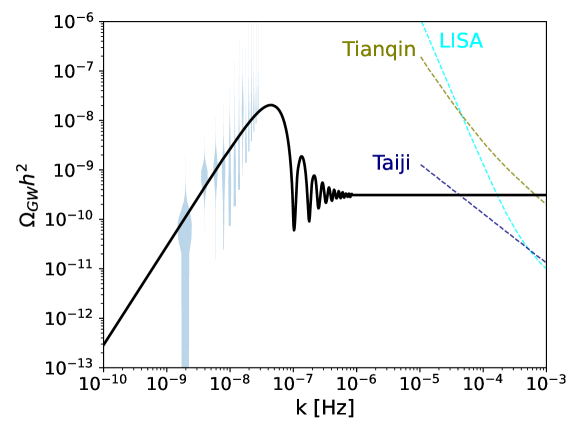
Figure 3: The spectral energy density parameter predicted by our model. The violin represents the NANOGrav result, and the dashed curves on the right represent the sensitivity of ongoing space-based GW detectors, including LISA Amaro-Seoane et al. (2017), Taiji Hu and Wu (2017) and TianQin Luo et al. (2016).

We present the spectral energy density parameter in Fig. 3. Our model not only exhibits a blue spectrum on the nHz scales, explaining the recent NanoGrav data, but also generates significant PGW signals on smaller scales, which might be probed by upcoming space-based GW detectors such as LISA, Taiji and TianQin. This distinctive feature could set our scenario apart from others. For instance, in the scalar-induced gravitational waves interpretation of PTA data Domènech (2020, 2021), the peaked gravitational wave signals are typically redshifted on scales smaller than the PTA scale, leading to undetectable signals on smaller scales. Consequently, our scenario could be distinguished from others through future experiments.

V Conclusion and Outlook

We examine whether the most up-to-date PTA results may offer insights into nonsingular cosmology. To achieve this, we investigate a toy Genesis-inflation model described by the action (1), which is able to yield a nearly scale-invariant scalar power spectrum. The tensor spectrum exhibits a blue tilt with $n_{T}=2$ over a wide frequency range, spanning from the observational window of the CMB to that of PTA. This characteristic allows for a direct comparison with PTA observations. Additionally, the amplitude of GWs could be substantial enough to be detectable by forthcoming space-based GW detectors, making our scenario potentially testable in the near future.

In this paper, we explore the aforementioned possibility through a toy Genesis-inflation model. There are many interesting questions to address in the forthcoming studies.

We need to account for scalar perturbations in the model. In Section III.4, we argue that the inflation epoch must be carefully treated to ensure a sizable PGW signal on the PTA scale while keeping the scalar perturbation small. This necessitates a relatively large tensor-to-scalar ratio $r$ or a breakdown of the consistency relation in canonical inflation. Thus, we will pay meticulous attention to the inflation (and the transition) epoch to ensure the safety of the scalar perturbation.

Additionally, we interpret the PTA observation as a result of amplified PGWs. As pointed out by Inomata et al. (2023), if the primordial scalar spectrum is amplified to certain scales, the back reaction at a non-linear level might be too strong to break the perturbation theory. Although the study focuses on scalar perturbation, a similar issue can potentially arise in our scenario. More specifically, to explain the PTA result through amplified PGWs, the tensor spectrum must have a minimal amplitude on PTA scales and smaller scales. It is essential to address, whether this minimal amplitude will always result in model-independent large back-reaction, or the back-reaction issue is dependent on the model construction.

Furthermore, we find that in our toy model, there is a potential trans-Planckian issue at high frequency band. It’s also known that Genesis cosmology might suffer from the strong coupling problem Ageeva et al. (2020, 2021); Akama and Hirano (2023). Further examination of healthier realization in nonsingular scenarios, such as the Ekpyrosis-bounce-inflation scenario, is necessary.

References

- Borde and Vilenkin (1994) A. Borde and A. Vilenkin, Phys. Rev. Lett. 72, 3305 (1994), arXiv:gr-qc/9312022 .
- Borde et al. (2003) A. Borde, A. H. Guth, and A. Vilenkin, Phys. Rev. Lett. 90, 151301 (2003), arXiv:gr-qc/0110012 .
- Lesnefsky et al. (2023) J. E. Lesnefsky, D. A. Easson, and P. C. W. Davies, Phys. Rev. D 107, 044024 (2023), arXiv:2207.00955 [gr-qc] .
- Geshnizjani et al. (2023) G. Geshnizjani, E. Ling, and J. Quintin, (2023), arXiv:2305.01676 [gr-qc] .
- Gasperini and Veneziano (1993) M. Gasperini and G. Veneziano, Astropart. Phys. 1, 317 (1993), arXiv:hep-th/9211021 .
- Finelli and Brandenberger (2002) F. Finelli and R. Brandenberger, Phys. Rev. D 65, 103522 (2002), arXiv:hep-th/0112249 .
- Piao et al. (2004) Y.-S. Piao, B. Feng, and X.-m. Zhang, Phys. Rev. D 69, 103520 (2004), arXiv:hep-th/0310206 .
- Piao (2004) Y.-S. Piao, Phys. Rev. D 70, 101302 (2004), arXiv:hep-th/0407258 .
- Piao (2005) Y.-S. Piao, Phys. Rev. D 71, 087301 (2005), arXiv:astro-ph/0502343 .
- Cai et al. (2007) Y.-F. Cai, T. Qiu, Y.-S. Piao, M. Li, and X. Zhang, JHEP 10, 071 (2007), arXiv:0704.1090 [gr-qc] .
- Cai et al. (2011) Y.-F. Cai, S.-H. Chen, J. B. Dent, S. Dutta, and E. N. Saridakis, Class. Quant. Grav. 28, 215011 (2011), arXiv:1104.4349 [astro-ph.CO] .
- Easson et al. (2011) D. A. Easson, I. Sawicki, and A. Vikman, JCAP 1111, 021 (2011), arXiv:1109.1047 [hep-th] .
- Cai et al. (2012) Y.-F. Cai, D. A. Easson, and R. Brandenberger, JCAP 08, 020 (2012), arXiv:1206.2382 [hep-th] .
- Liu et al. (2013) Z.-G. Liu, Z.-K. Guo, and Y.-S. Piao, Phys. Rev. D 88, 063539 (2013), arXiv:1304.6527 [astro-ph.CO] .
- Qiu et al. (2013) T. Qiu, X. Gao, and E. N. Saridakis, Phys. Rev. D 88, 043525 (2013), arXiv:1303.2372 [astro-ph.CO] .
- Koehn et al. (2014) M. Koehn, J.-L. Lehners, and B. A. Ovrut, Phys. Rev. D 90, 025005 (2014), arXiv:1310.7577 [hep-th] .
- Wan et al. (2015) Y. Wan, T. Qiu, F. P. Huang, Y.-F. Cai, H. Li, and X. Zhang, JCAP 12, 019 (2015), arXiv:1509.08772 [gr-qc] .
- Qiu and Wang (2015) T. Qiu and Y.-T. Wang, JHEP 04, 130 (2015), arXiv:1501.03568 [astro-ph.CO] .
- Nojiri et al. (2016) S. Nojiri, S. D. Odintsov, and V. K. Oikonomou, Phys. Rev. D 93, 084050 (2016), arXiv:1601.04112 [gr-qc] .
- Banerjee and Saridakis (2017) S. Banerjee and E. N. Saridakis, Phys. Rev. D 95, 063523 (2017), arXiv:1604.06932 [gr-qc] .
- Chen et al. (2018) J.-W. Chen, C.-H. Li, Y.-B. Li, and M. Zhu, Sci. China Phys. Mech. Astron. 61, 100411 (2018), arXiv:1711.10897 [physics.gen-ph] .
- Mironov et al. (2018) S. Mironov, V. Rubakov, and V. Volkova, JCAP 10, 050 (2018), arXiv:1807.08361 [hep-th] .
- Akama and Kobayashi (2019) S. Akama and T. Kobayashi, Phys. Rev. D 99, 043522 (2019), arXiv:1810.01863 [gr-qc] .
- Ye and Piao (2019a) G. Ye and Y.-S. Piao, Commun. Theor. Phys. 71, 427 (2019a), arXiv:1901.02202 [gr-qc] .
- Akama et al. (2020) S. Akama, S. Hirano, and T. Kobayashi, Phys. Rev. D 101, 043529 (2020), arXiv:1908.10663 [gr-qc] .
- Ye and Piao (2019b) G. Ye and Y.-S. Piao, Phys. Rev. D 99, 084019 (2019b), arXiv:1901.08283 [gr-qc] .
- Mironov et al. (2020) S. Mironov, V. Rubakov, and V. Volkova, JCAP 05, 024 (2020), arXiv:1910.07019 [hep-th] .
- Nandi and Sriramkumar (2020) D. Nandi and L. Sriramkumar, Phys. Rev. D 101, 043506 (2020), arXiv:1904.13254 [gr-qc] .
- Nandi (2021) D. Nandi, Universe 7, 62 (2021), arXiv:2009.03134 [gr-qc] .
- Battista (2021) E. Battista, Class. Quant. Grav. 38, 195007 (2021), arXiv:2011.09818 [gr-qc] .
- Zhu et al. (2021) M. Zhu, A. Ilyas, Y. Zheng, Y.-F. Cai, and E. N. Saridakis, JCAP 11, 045 (2021), arXiv:2108.01339 [gr-qc] .
- Banerjee et al. (2022) I. Banerjee, T. Paul, and S. SenGupta, Gen. Rel. Grav. 54, 119 (2022), arXiv:2205.05283 [gr-qc] .
- Ganz et al. (2023) A. Ganz, P. Martens, S. Mukohyama, and R. Namba, JCAP 04, 060 (2023), arXiv:2212.13561 [gr-qc] .
- Zhu and Cai (2023) M. Zhu and Y. Cai, JHEP 04, 095 (2023), arXiv:2301.13502 [gr-qc] .
- Singh et al. (2023) J. K. Singh, Shaily, A. Singh, A. Beesham, and H. Shabani, Annals Phys. 455, 169382 (2023), arXiv:2304.11578 [gr-qc] .
- Burkmar and Bruni (2023) M. Burkmar and M. Bruni, Phys. Rev. D 107, 083533 (2023), arXiv:2302.03710 [gr-qc] .
- Kaur et al. (2023) M. Kaur, D. Nandi, D. Choudhury, and T. R. Seshadri, (2023), arXiv:2302.13698 [astro-ph.CO] .
- Tripathy et al. (2023) S. K. Tripathy, S. K. Pradhan, B. Barik, Z. Naik, and B. Mishra, Symmetry 15, 790 (2023), arXiv:2303.12168 [gr-qc] .
- Creminelli et al. (2010) P. Creminelli, A. Nicolis, and E. Trincherini, JCAP 11, 021 (2010), arXiv:1007.0027 [hep-th] .
- Liu et al. (2011) Z.-G. Liu, J. Zhang, and Y.-S. Piao, Phys. Rev. D 84, 063508 (2011), arXiv:1105.5713 [astro-ph.CO] .
- Wang and Brandenberger (2012) Y. Wang and R. Brandenberger, JCAP 10, 021 (2012), arXiv:1206.4309 [hep-th] .
- Liu and Piao (2013) Z.-G. Liu and Y.-S. Piao, Phys. Lett. B 718, 734 (2013), arXiv:1207.2568 [gr-qc] .
- Creminelli et al. (2013) P. Creminelli, K. Hinterbichler, J. Khoury, A. Nicolis, and E. Trincherini, JHEP 02, 006 (2013), arXiv:1209.3768 [hep-th] .
- Hinterbichler et al. (2012) K. Hinterbichler, A. Joyce, J. Khoury, and G. E. J. Miller, JCAP 12, 030 (2012), arXiv:1209.5742 [hep-th] .
- Hinterbichler et al. (2013) K. Hinterbichler, A. Joyce, J. Khoury, and G. E. J. Miller, Phys. Rev. Lett. 110, 241303 (2013), arXiv:1212.3607 [hep-th] .
- Easson et al. (2013) D. A. Easson, I. Sawicki, and A. Vikman, JCAP 1307, 014 (2013), arXiv:1304.3903 [hep-th] .
- Liu et al. (2014) Z.-G. Liu, H. Li, and Y.-S. Piao, Phys. Rev. D 90, 083521 (2014), arXiv:1405.1188 [astro-ph.CO] .
- Pirtskhalava et al. (2014) D. Pirtskhalava, L. Santoni, E. Trincherini, and P. Uttayarat, JHEP 12, 151 (2014), arXiv:1410.0882 [hep-th] .
- Nishi and Kobayashi (2015) S. Nishi and T. Kobayashi, JCAP 03, 057 (2015), arXiv:1501.02553 [hep-th] .
- Cai and Piao (2016) Y. Cai and Y.-S. Piao, JHEP 03, 134 (2016), arXiv:1601.07031 [hep-th] .
- Nishi and Kobayashi (2017) S. Nishi and T. Kobayashi, Phys. Rev. D 95, 064001 (2017), arXiv:1611.01906 [hep-th] .
- Dobre et al. (2018) D. A. Dobre, A. V. Frolov, J. T. G. Ghersi, S. Ramazanov, and A. Vikman, JCAP 03, 020 (2018), arXiv:1712.10272 [gr-qc] .
- Mironov et al. (2019) S. Mironov, V. Rubakov, and V. Volkova, Phys. Rev. D 100, 083521 (2019), arXiv:1905.06249 [hep-th] .
- Zhu and Zheng (2021) M. Zhu and Y. Zheng, JHEP 11, 163 (2021), arXiv:2109.05277 [gr-qc] .
- Cai et al. (2022) Y. Cai, J. Xu, S. Zhao, and S. Zhou, JHEP 10, 140 (2022), [Erratum: JHEP 11, 063 (2022)], arXiv:2207.11772 [gr-qc] .
- Piao and Zhou (2003) Y.-S. Piao and E. Zhou, Phys. Rev. D 68, 083515 (2003), arXiv:hep-th/0308080 .
- Piao (2007) Y.-S. Piao, Phys. Rev. D 76, 083505 (2007), arXiv:0706.0981 [gr-qc] .
- Khoury et al. (2001) J. Khoury, B. A. Ovrut, P. J. Steinhardt, and N. Turok, Phys. Rev. D 64, 123522 (2001), arXiv:hep-th/0103239 .
- Boyle et al. (2004) L. A. Boyle, P. J. Steinhardt, and N. Turok, Phys. Rev. D 69, 127302 (2004), arXiv:hep-th/0307170 .
- Qiu et al. (2011) T. Qiu, J. Evslin, Y.-F. Cai, M. Li, and X. Zhang, JCAP 10, 036 (2011), arXiv:1108.0593 [hep-th] .
- Nishi and Kobayashi (2016) S. Nishi and T. Kobayashi, JCAP 04, 018 (2016), arXiv:1601.06561 [hep-th] .
- Piao and Zhang (2004a) Y.-S. Piao and Y.-Z. Zhang, Phys. Rev. D 70, 063513 (2004a), arXiv:astro-ph/0401231 .
- Wang and Xue (2014) Y. Wang and W. Xue, JCAP 10, 075 (2014), arXiv:1403.5817 [astro-ph.CO] .
- Cai et al. (2016a) Y. Cai, Y.-T. Wang, and Y.-S. Piao, Phys. Rev. D 93, 063005 (2016a), arXiv:1510.08716 [astro-ph.CO] .
- Cai et al. (2016b) Y. Cai, Y.-T. Wang, and Y.-S. Piao, Phys. Rev. D 94, 043002 (2016b), arXiv:1602.05431 [astro-ph.CO] .
- Wang et al. (2017) Y.-T. Wang, Y. Cai, Z.-G. Liu, and Y.-S. Piao, JCAP 01, 010 (2017), arXiv:1612.05088 [astro-ph.CO] .
- Cai and Piao (2021) Y. Cai and Y.-S. Piao, Phys. Rev. D 103, 083521 (2021), arXiv:2012.11304 [gr-qc] .
- Cai and Piao (2022) Y. Cai and Y.-S. Piao, JHEP 06, 067 (2022), arXiv:2201.04552 [gr-qc] .
- Afzal et al. (2023) A. Afzal et al. (NANOGrav), Astrophys. J. Lett. 951, L11 (2023), arXiv:2306.16219 [astro-ph.HE] .
- Agazie et al. (2023) G. Agazie et al. (NANOGrav), Astrophys. J. Lett. 951, L8 (2023), arXiv:2306.16213 [astro-ph.HE] .
- Antoniadis et al. (2023a) J. Antoniadis et al., (2023a), arXiv:2306.16214 [astro-ph.HE] .
- Reardon et al. (2023) D. J. Reardon et al., Astrophys. J. Lett. 951, L6 (2023), arXiv:2306.16215 [astro-ph.HE] .
- Xu et al. (2023) H. Xu et al., Res. Astron. Astrophys. 23, 075024 (2023), arXiv:2306.16216 [astro-ph.HE] .
- Antoniadis et al. (2023b) J. Antoniadis et al., (2023b), arXiv:2306.16227 [astro-ph.CO] .
- Vagnozzi (2023) S. Vagnozzi, JHEAp 39, 81 (2023), arXiv:2306.16912 [astro-ph.CO] .
- Piao and Zhang (2004b) Y.-S. Piao and Y.-Z. Zhang, Phys. Rev. D 70, 043516 (2004b), arXiv:astro-ph/0403671 .
- Huang et al. (2023) H.-L. Huang, Y. Cai, J.-Q. Jiang, J. Zhang, and Y.-S. Piao, (2023), arXiv:2306.17577 [gr-qc] .
- Madge et al. (2023) E. Madge, E. Morgante, C. Puchades-Ibáñez, N. Ramberg, W. Ratzinger, S. Schenk, and P. Schwaller, (2023), arXiv:2306.14856 [hep-ph] .
- Ellis et al. (2023a) J. Ellis, M. Fairbairn, G. Hütsi, J. Raidal, J. Urrutia, V. Vaskonen, and H. Veermäe, (2023a), arXiv:2306.17021 [astro-ph.CO] .
- Ellis et al. (2023b) J. Ellis, M. Lewicki, C. Lin, and V. Vaskonen, (2023b), arXiv:2306.17147 [astro-ph.CO] .
- Franciolini et al. (2023) G. Franciolini, A. Iovino, Junior., V. Vaskonen, and H. Veermae, (2023), arXiv:2306.17149 [astro-ph.CO] .
- Zhang et al. (2023a) C. Zhang, N. Dai, Q. Gao, Y. Gong, T. Jiang, and X. Lu, (2023a), arXiv:2307.01093 [gr-qc] .
- Cannizzaro et al. (2023) E. Cannizzaro, G. Franciolini, and P. Pani, (2023), arXiv:2307.11665 [gr-qc] .
- Zhang et al. (2023b) Z. Zhang, C. Cai, Y.-H. Su, S. Wang, Z.-H. Yu, and H.-H. Zhang, (2023b), arXiv:2307.11495 [hep-ph] .
- Balaji et al. (2023) S. Balaji, G. Domènech, and G. Franciolini, (2023), arXiv:2307.08552 [gr-qc] .
- Du et al. (2023) X. K. Du, M. X. Huang, F. Wang, and Y. K. Zhang, (2023), arXiv:2307.02938 [hep-ph] .
- Zhu et al. (2023) Q.-H. Zhu, Z.-C. Zhao, and S. Wang, (2023), arXiv:2307.03095 [astro-ph.CO] .
- Shen et al. (2023) Z.-Q. Shen, G.-W. Yuan, Y.-Y. Wang, and Y.-Z. Wang, (2023), arXiv:2306.17143 [astro-ph.HE] .
- Di Bari and Rahat (2023) P. Di Bari and M. H. Rahat, (2023), arXiv:2307.03184 [hep-ph] .
- Li and Xie (2023) S.-P. Li and K.-P. Xie, (2023), arXiv:2307.01086 [hep-ph] .
- Li (2023) X.-F. Li, (2023), arXiv:2307.03163 [hep-ph] .
- Konoplya and Zhidenko (2023) R. A. Konoplya and A. Zhidenko, (2023), arXiv:2307.01110 [gr-qc] .
- Niu and Rahat (2023) X. Niu and M. H. Rahat, (2023), arXiv:2307.01192 [hep-ph] .
- Ghosh et al. (2023) T. Ghosh, A. Ghoshal, H.-K. Guo, F. Hajkarim, S. F. King, K. Sinha, X. Wang, and G. White, (2023), arXiv:2307.02259 [astro-ph.HE] .
- Wang et al. (2023) S. Wang, Z.-C. Zhao, J.-P. Li, and Q.-H. Zhu, (2023), arXiv:2307.00572 [astro-ph.CO] .
- Wu et al. (2023) Y.-M. Wu, Z.-C. Chen, and Q.-G. Huang, (2023), arXiv:2307.03141 [astro-ph.CO] .
- Liu et al. (2023a) L. Liu, Z.-C. Chen, and Q.-G. Huang, (2023a), arXiv:2307.01102 [astro-ph.CO] .
- Liu et al. (2023b) L. Liu, Z.-C. Chen, and Q.-G. Huang, (2023b), arXiv:2307.14911 [astro-ph.CO] .
- Jiang et al. (2023a) S. Jiang, A. Yang, J. Ma, and F. P. Huang, (2023a), arXiv:2306.17827 [hep-ph] .
- Cai et al. (2023) Y.-F. Cai, X.-C. He, X. Ma, S.-F. Yan, and G.-W. Yuan, (2023), arXiv:2306.17822 [gr-qc] .
- Addazi et al. (2023) A. Addazi, Y.-F. Cai, A. Marciano, and L. Visinelli, (2023), arXiv:2306.17205 [astro-ph.CO] .
- Bian et al. (2023) L. Bian, S. Ge, J. Shu, B. Wang, X.-Y. Yang, and J. Zong, (2023), arXiv:2307.02376 [astro-ph.HE] .
- Han et al. (2023) C. Han, K.-P. Xie, J. M. Yang, and M. Zhang, (2023), arXiv:2306.16966 [hep-ph] .
- Guo et al. (2023) S.-Y. Guo, M. Khlopov, X. Liu, L. Wu, Y. Wu, and B. Zhu, (2023), arXiv:2306.17022 [hep-ph] .
- Ye and Silvestri (2023) G. Ye and A. Silvestri, (2023), arXiv:2307.05455 [astro-ph.CO] .
- Jiang et al. (2023b) J.-Q. Jiang, Y. Cai, G. Ye, and Y.-S. Piao, (2023b), arXiv:2307.15547 [astro-ph.CO] .
- Choudhury (2023) S. Choudhury, (2023), arXiv:2307.03249 [astro-ph.CO] .
- Cheung et al. (2023) K. Cheung, C. J. Ouseph, and P.-Y. Tseng, (2023), arXiv:2307.08046 [hep-ph] .
- Oikonomou (2023a) V. K. Oikonomou, (2023a), arXiv:2306.17351 [astro-ph.CO] .
- Sakharov et al. (2021) A. S. Sakharov, Y. N. Eroshenko, and S. G. Rubin, Phys. Rev. D 104, 043005 (2021), arXiv:2104.08750 [hep-ph] .
- Ashoorioon et al. (2022) A. Ashoorioon, K. Rezazadeh, and A. Rostami, Phys. Lett. B 835, 137542 (2022), arXiv:2202.01131 [astro-ph.CO] .
- Lazarides et al. (2023) G. Lazarides, R. Maji, and Q. Shafi, (2023), arXiv:2306.17788 [hep-ph] .
- Odintsov et al. (2022) S. D. Odintsov, V. K. Oikonomou, and F. P. Fronimos, Phys. Dark Univ. 35, 100950 (2022), arXiv:2108.11231 [gr-qc] .
- Oikonomou (2022) V. K. Oikonomou, Nucl. Phys. B 984, 115985 (2022), arXiv:2210.02861 [gr-qc] .
- Oikonomou (2023b) V. K. Oikonomou, Phys. Rev. D 107, 064071 (2023b), arXiv:2303.05889 [hep-ph] .
- Cai et al. (2017a) Y. Cai, H.-G. Li, T. Qiu, and Y.-S. Piao, Eur. Phys. J. C 77, 369 (2017a), arXiv:1701.04330 [gr-qc] .
- Amaro-Seoane et al. (2017) P. Amaro-Seoane et al. (LISA), (2017), arXiv:1702.00786 [astro-ph.IM] .
- Hu and Wu (2017) W.-R. Hu and Y.-L. Wu, Natl. Sci. Rev. 4, 685 (2017).
- Luo et al. (2016) J. Luo et al. (TianQin), Class. Quant. Grav. 33, 035010 (2016), arXiv:1512.02076 [astro-ph.IM] .
- Libanov et al. (2016) M. Libanov, S. Mironov, and V. Rubakov, JCAP 08, 037 (2016), arXiv:1605.05992 [hep-th] .
- Kobayashi (2016) T. Kobayashi, Phys. Rev. D 94, 043511 (2016), arXiv:1606.05831 [hep-th] .
- Cai et al. (2017b) Y. Cai, Y. Wan, H.-G. Li, T. Qiu, and Y.-S. Piao, JHEP 01, 090 (2017b), arXiv:1610.03400 [gr-qc] .
- Creminelli et al. (2016) P. Creminelli, D. Pirtskhalava, L. Santoni, and E. Trincherini, JCAP 11, 047 (2016), arXiv:1610.04207 [hep-th] .
- Cai and Piao (2017) Y. Cai and Y.-S. Piao, JHEP 09, 027 (2017), arXiv:1705.03401 [gr-qc] .
- Kolevatov et al. (2017) R. Kolevatov, S. Mironov, N. Sukhov, and V. Volkova, JCAP 08, 038 (2017), arXiv:1705.06626 [hep-th] .
- Ilyas et al. (2021) A. Ilyas, M. Zhu, Y. Zheng, and Y.-F. Cai, JHEP 01, 141 (2021), arXiv:2009.10351 [gr-qc] .
- Ilyas et al. (2020) A. Ilyas, M. Zhu, Y. Zheng, Y.-F. Cai, and E. N. Saridakis, JCAP 09, 002 (2020), arXiv:2002.08269 [gr-qc] .
- Brandenberger and Martin (2001) R. H. Brandenberger and J. Martin, Mod. Phys. Lett. A 16, 999 (2001), arXiv:astro-ph/0005432 .
- Martin and Brandenberger (2001) J. Martin and R. H. Brandenberger, Phys. Rev. D 63, 123501 (2001), arXiv:hep-th/0005209 .
- Domènech (2020) G. Domènech, Int. J. Mod. Phys. D 29, 2050028 (2020), arXiv:1912.05583 [gr-qc] .
- Domènech (2021) G. Domènech, Universe 7, 398 (2021), arXiv:2109.01398 [gr-qc] .
- Inomata et al. (2023) K. Inomata, M. Braglia, X. Chen, and S. Renaux-Petel, JCAP 04, 011 (2023), arXiv:2211.02586 [astro-ph.CO] .
- Ageeva et al. (2020) Y. Ageeva, P. Petrov, and V. Rubakov, JHEP 12, 107 (2020), arXiv:2009.05071 [hep-th] .
- Ageeva et al. (2021) Y. Ageeva, P. Petrov, and V. Rubakov, Phys. Rev. D 104, 063530 (2021), arXiv:2104.13412 [hep-th] .
- Akama and Hirano (2023) S. Akama and S. Hirano, Phys. Rev. D 107, 063504 (2023), arXiv:2211.00388 [gr-qc] .