Energy Transfer and Radiation in Hamiltonian Nonlinear Klein-Gordon Equations: General Case

Abstract

In this paper, we consider Klein-Gordon equations with cubic nonlinearity in three spatial dimensions, which are Hamiltonian perturbations of the linear one with potential. It is assumed that the corresponding Klein-Gordon operator $B=\sqrt{-\Delta+V(x)+m^{2}}$ admits an arbitrary number of possibly degenerate eigenvalues in $(0,m)$, and hence the unperturbed linear equation has multiple time-periodic solutions known as bound states. In [37], Soffer and Weinstein discovered a mechanism called Fermi’s Golden Rule for this nonlinear system in the case of one simple but relatively large eigenvalue $\Omega\in(\frac{m}{3},m)$, by which energy is transferred from discrete to continuum modes and the solution still decays in time. In particular, the exact energy transfer rate is given. In [25], we solved the general one simple eigenvalue case. In this paper, we solve this problem in full generality: multiple and simple or degenerate eigenvalues in $(0,m)$. The proof is based on a kind of pseudo-one-dimensional cancellation structure in each eigenspace, a renormalized damping mechanism, and an enhanced damping effect. It also relies on a refined Birkhoff normal form transformation and an accurate generalized Fermi’s Golden Rule over those of Bambusi–Cuccagna [3].

1 Introduction

We consider the Klein-Gordon equation with an external potential $V$ and a cubic nonlinearity in $3+1$ dimensions:

$$\begin{cases}\partial^{2}_{t}u-\Delta u+m^{2}u+V(x)u=\lambda u^{3},&t>0,x\in\mathbb{R}^{3},\lambda\in\mathbb{R},\\ u(x,0)=u_{0}(x),\quad\partial_{t}u(x,0)=u_{1}(x).\end{cases}$$ (1.1)

The potential function $V$ is assumed to be real-valued, smooth and sufficiently fast decaying. Thus, the corresponding Schrödinger operator $H=-\Delta+V$ has purely absolutely continuous spectrum $[0,+\infty)$ and a finite number of negative eigenvalues [33]. We denote these eigenvalues to be $0>\lambda_{1}>\lambda_{2}>\dots>\lambda_{n}$, with each eigenvalue $\lambda_{j}$ the corresponding $l_{j}$ dimensional eigenspace is spanned by an orthonormal basis $\{\varphi_{j1},\dots,\varphi_{jl_{j}}\}$. These eigenfunctions are smooth and fast decaying, see [33]. We take a mass term $m^{2}$ such that $-\Delta+V+m^{2}>0$. Set $B=\sqrt{-\Delta+V+m^{2}}$ and $\omega_{j}=\sqrt{m^{2}+\lambda_{j}}$, then $B$ has purely absolutely continuous spectrum $[m,+\infty)$ and $n$ distinct eigenvalues $m>\omega_{1}>\omega_{2}>\dots>\omega_{n}>0$.

In this setting, the linear equation, i.e. (1.1) with $\lambda=0$, possesses a family of time-periodic solutions

$$u(t,x)=A\cos(\omega_{j}t+\theta)\varphi_{jk}(x),$$

for $1\leq j\leq n$, $1\leq k\leq l_{j}$ and $A,\theta\in\mathbb{R}$. In quantum mechanics, these periodic solutions are known as bound states. Under a small nonlinear perturbation, an excited state could be unstable with energy shifting to the ground state, free waves and nearby excited states. However, it has been observed that in the meanwhile an anomalously long-lived state, known as metastable state, exists [2, 35, 36, 37]. Thus, an interesting question is to investigate the long time behavior of these bound states especially under small Hamiltonian nonlinear perturbations. In particular, it is crucial to give a precise description on the mechanism and the rate that energy transfers from bound states to free waves. Besides, it is worth noting that this type of equations we consider in this paper appear naturally when studying the asymptotic stability of special solutions of nonlinear dispersive and hyperbolic equations, such as solitons, traveling waves, kinks. For instance see [14, 23, 24, 26].

The rigorous mathematical analysis of such phenomenons began in the 1990s. In 1993, Sigal [32] first established the instability mechanism of quasi-periodic solutions to nonlinear Schrödinger and wave equations in a qualitative manner, in which the Fermi’s Golden Rule was first introduced and explored in the field of analysis and partial differential equations. In 1999, Soffer and Weinstein [37] made a significant progress and discovered the Fermi’s Golden Rule for the Klein-Gordon equation (1.1). They proved that if the operator $B$ has one simple eigenvalue $\omega$ satisfying $3\omega>m$, then the Fermi’s Golden Rule plays an instability role and small global solutions to (1.1) decay to zero at an anomalously slow rate as time tends to infinity. In particular, an accurate energy transfer rate from discrete to continuum modes is given. More precisely, the solution $u(t,x)$ has the following expansion as $t\to\pm\infty$:

$$u(t,x)=R(t)\cos(\omega t+\theta(t))\varphi(x)+\eta(t,x),$$ (1.2)

where

$$R(t)=\mathcal{O}(|t|^{-\frac{1}{4}}),\theta(t)=\mathcal{O}(|t|^{\frac{1}{2}}),\quad\|\eta(t,\cdot)\|_{L^{8}}=\mathcal{O}(|t|^{-\frac{3}{4}}).$$

The lower bound of the decay rate has later been proved using an alternative approach by An–Soffer [2]. In the recent interesting work [26], Leger and Pusateri extended the results of [37] to quadratic nonlinearity and obtained the sharp decay rate. We point out that the general case with multiple and simple or degenerate eigenvalue case is left open, see the discussions in [3, 37].

In [25], the authors of this paper solved the problem in the one simple eigenvalue case, i.e. in the weak resonance regime $(2N-1)\omega<m<(2N+1)\omega$ with any given integer $N\geq 1$. The proof relies on the discovery of a generalized Fermi’s Golden Rule and certain weighted dispersive estimates. More precisely, it is shown that the expansion (1.2) of global solution $u(t,x)$ still holds with following quantitative estimates:

$$\frac{\frac{1}{C}R(0)}{(1+4N\lambda^{2N}|R(0)|^{4N}\gamma t)^{\frac{1}{4N}}}\leq R(t)\leq\frac{CR(0)}{(1+4N\lambda^{2N}|R(0)|^{4N}\gamma t)^{\frac{1}{4N}}},$$

$$\theta(t)=\mathcal{O}(|t|^{1-\frac{1}{2N}}),\quad\|\eta(t,\cdot)\|_{L^{8}}=\mathcal{O}(|t|^{-\frac{3}{4N}}).$$

for some positive constant $C>0$.

In this paper, we solve this problem in full generality: multiple and simple or degenerate eigenvalues in $(0,m)$. The proof is based on a kind of pseudo-one-dimensional cancellation structure in each eigenspace, a renormalized damping mechanism and an enhanced damping effect for the norms of discrete modes. It also relies on a refined Birkhoff normal form transformation and an accurate generalized Fermi’s Golden Rule over those of Bambusi–Cuccagna [3]. See Theorem 1.2 and next subsection for more details.

These results give a theoretic verification that an excited state could be unstable with energy shifting to the ground state, free waves and nearby excited states under small Hamiltonian perturbations. The underlying mechanism is a kind of generalized Fermi’s Golden Rule, see Assumption 5.5. They also provide a quantitative description on the energy transfer from discrete to continuum modes and on the radiation of continuum modes. As a corollary, there are no small global periodic or quasi-periodic solutions to (1.1) under the generalized Fermi’s Golden Rule. We mention that the Fermi’s Golden Rule has also been used to study the asymptotic stability of solitons of nonlinear Schrödinger equations by Tsai–Yau [40], Soffer–Weinstein [38], Gang [11], Gang–Sigal [12], Gang–Weinstein [13]; see also the recent advances by Cuccagna–Maeda [7], their survey [8] and references therein.

Let us mention that when the operator $B$ has multiple eigenvalues in general case, the first progress is made by Bambusi and Cuccagana [3], where they proved that solutions of (1.1) with small initial data in $H^{1}\times L^{2}$ are asymptotically free under a non-degeneracy hypothesis. We note that the energy transfer rate can not be proved for $H^{1}\times L^{2}$ initial data due to the conservation of energy. Indeed, the authors in [3] conjectured that appropriate decay rates are reachable if restricting initial data to certain class like that of Soffer-Weinstein [37].

We also mention that the phenomenon here is reminiscent of the famous Kolmogorov-Arnold-Moser (KAM) theory, which is concerned with the persistence of periodic and quasi-periodic motion under the Hamiltonian perturbation of a dynamical system. For a finite dimensional integrable Hamiltonian system, this was initiated by Kolmogorov [19] and then extended by Moser [27] and Arnold [1]. Subsequently, many efforts have been focused on generalizing the KAM theory to infinite dimensional Hamiltonian systems (Hamiltonian PDEs), wherein solutions are defined on compact spatial domains, such as [5, 9, 20]. In all these results, appropriate non-resonance conditions imply the persistence of periodic and quasi-periodic solutions. See [22, 41] and the references therein for a comprehensive survey. However, the results here (and also in [37, 25], etc.) show that a different scenario happens for Hamiltonian PDEs in the whole space, i.e. resonance conditions lead to the instability of periodic or quasi-periodic solutions.

1.1 Main Result

Before presenting the main result of this paper, we first state our assumptions:

Assumption 1.1.

Assume that the Schrödinger operator $H=-\Delta+V$ satisfies the following conditions:
(V1) $V$ is real-valued, smooth and decays sufficiently fast;
(V2) $0$ is not a resonance nor an eigenvalue of the operator $-\Delta+V$;
(V3) For each $\omega_{j}$, there exists an integer $N_{j}$ such that $\frac{m}{2N_{j}+1}<\omega_{j}<\frac{m}{2N_{j}-1}$, with $1\leq N_{1}\leq N_{2}\leq\dots\leq N_{n}$;
(V4) For any $\mu\in\mathbb{Z}^{n}$ with $|\mu|\leq 100N_{n}$ and $|\mu|$ being odd, $\sum_{j=1}^{n}\mu_{j}\omega_{j}\neq m$;
(V5) For any $\mu\in\mathbb{Z}^{n}$ with $|\mu|\leq 100N_{n}$ and $|\mu|$ being even, $\sum_{j=1}^{n}\mu_{j}\omega_{j}=0$ implies $\mu=0$;
(V6) The generalized Fermi’s Gordon Rule condition holds, i.e. Assumption 5.5 holds.

Denote $\mathbf{P}_{c}$ to be the projection onto the continuous spectral part of $B$, then any solution $u$ of the equation (1.1) has the following decomposition:

$$u=\sum_{j=1}^{n}\sum_{k=1}^{l_{j}}q_{jk}\varphi_{jk}+\mathbf{P}_{c}u,$$ (1.3)

where $q_{jk}(t):=\langle u,\varphi_{jk}\rangle$. We also define

$$\|u\|_{X}:=\|u\|_{W^{100N_{n},1}}+\|u\|_{W^{100N_{n},2}}.$$

The main result of this paper is as follows.

Theorem 1.2.

Under assumptions (V1)-(V6), there exists a small constant $\epsilon_{0}>0$ such that for any $0<\epsilon\leq\epsilon_{0}$, if the initial data satisfies

$$\|u_{0}\|_{X}+\|u_{1}\|_{X}=\epsilon,$$ (1.4)

$$\sum_{k=1}^{l_{j}}\left(|q_{jk}(0)|+|q^{\prime}_{jk}(0)|\right)\lesssim\epsilon^{\alpha_{j}},\quad\forall~{}1\leq j\leq n,$$ (1.5)

$$\|\mathbf{P}_{c}u_{0}\|_{X}+\|\mathbf{P}_{c}u_{1}\|_{X}\lesssim\epsilon^{3},$$ (1.6)

where $\alpha_{j}=\min\left\{\frac{N_{n}}{N_{j}},3\right\}$, then

$$\sum_{k=1}^{l_{j}}\left(|q_{jk}(t)|+|q^{\prime}_{jk}(t)|\right)\lesssim\frac{\epsilon^{\alpha_{j}}}{\left(1+\epsilon^{4N_{n}}t\right)^{\frac{\alpha_{j}}{4N_{n}}}},\quad\forall~{}1\leq j\leq n$$ (1.7)

$$\|\mathbf{P}_{c}u\|_{\infty}+\|\mathbf{P}_{c}\partial_{t}u\|_{\infty}\lesssim\frac{\epsilon^{3}}{\left(1+\epsilon^{4N_{n}}t\right)^{\frac{3}{4N_{n}}}},$$ (1.8)

$$\|\mathbf{P}_{d}u\|_{X}\approx\frac{\epsilon}{\left(1+\epsilon^{4N_{n}}t\right)^{\frac{1}{4N_{n}}}},\quad\mathbf{P}_{d}\triangleq 1-\mathbf{P}_{c}.$$ (1.9)

Remark 1.3.

By (1.8) and (1.9), we obtain that the sharp decay rate of $u$ is

$$\|u\|_{\infty}\approx\frac{\epsilon}{\left(1+\epsilon^{4N_{n}}t\right)^{\frac{1}{4N_{n}}}}.$$

For $n=1$, this is reduced to the one simple eigenvalue case considered in [25], which is further reduced to [37] when $N_{n}=1$.

Remark 1.4.

We indicate that the assumption on initial data

$$\sum_{k=1}^{l_{j}}\left(|q_{jk}(0)|+|q^{\prime}_{jk}(0)|\right)\lesssim\epsilon^{\alpha_{j}},\quad\forall~{}1\leq j\leq n,$$

is to ensure that the discrete mode with slowest decay dominates at the initial time, which is a technical issue for our perturbation argument to derive the lower bound of $u$. Assumptions like (1.6) is necessary, which leads to resonance-dominated solutions with the decay rates $\langle t\rangle^{-\frac{1}{4N_{n}}}$ . Otherwise, there may exist dispersion-dominated solutions with faster decay rates as pointed out by Tsai and Yau in [40]. However, It is worth noting that if we only want to get the upper bound of $u$, then (1.4) (without (1.5) and (1.6)) is enough. In this case, by slightly modifying the proofs in Section 7 and Section 8, we can still obtain

$$\|\mathbf{P}_{d}u\|_{X}\lesssim\frac{\epsilon}{\left(1+\epsilon^{4N_{n}}t\right)^{\frac{1}{4N_{n}}}},$$

$$\|\mathbf{P}_{c}u\|_{\infty}+\|\mathbf{P}_{c}\partial_{t}u\|_{\infty}\lesssim\frac{\epsilon^{3}}{\left(1+\epsilon^{4N_{n}}t\right)^{\frac{3}{4N_{n}}}}+\epsilon\langle t\rangle^{-\frac{3}{2}}.$$

Remark 1.5.

The choice of $\alpha_{j}$ is due to the normal form transformation. Since we only have $|\xi-\xi^{\prime}|\lesssim|\xi|^{3}$(see (3.3)), the best result we can get is $|\xi^{\prime}_{jk}|\lesssim|\xi^{\prime}|^{3}$. Essentially, this is the consequence of cubic nonlinear interactions. See Section 3 for details and relevant notations.

Remark 1.6.

The choice of norm $X$ can be weakened. Here we take $100N_{n}$ for the convenience of presentation of our proof.

1.2 Difficluties, New Ingredients and the Sketch of the Proof

Now we explain the main difficulties of this problem and our ideas and strategies. Without loss of generality, we set $\lambda=1$.

1.2.1 Resonance and Normal Form Transformation

As illustrated in [3], the energy transfer from discrete to continuum modes in [37], for the case when there exists only one simple eigenvalue lying close to the continuous spectrum, is due to nonlinear coupling. Technically speaking, this occurs because the equation of the discrete mode has a key coefficient with a positive sign, being called Fermi’s Golden Rule, which yields radiation. For the case when the eigenvalues of $B$ are not close to the continuous spectrum, however, the crucial coefficients in the equations of the discrete modes consist of terms of several different forms with indefinite sign, if one follows the non-Hamiltonian scheme of [37]. To overcome this difficulty, Bambusi–Cuccagna [3] introduced a novel Birkhoff normal form transformation, which preserves the Hamiltonian structure of (1.1). As we remarked in [25], for the cubic nonlinearity $u^{3}$, this new normal form transformation can be done more delicately to make the results consistent with the non-Hamiltonian method in [37]. Actually, we found that the order of normal form is increased by two in each step, which has already been observed in the one simple eigenvalue case in [25].

In this paper, we further refine the Birkhoff normal form transformation in [3] and obtain a generalization of the transformation in [25] to the multiple eigenvalues case. To illustrate, we write the nonlinear Klein-Gordon equations (1.1) as the following Hamilton equations (see Section 3 for details)

$$\dot{\xi}_{jk} =-\mathrm{i}\partial_{\bar{\xi}_{jk}}H,\quad 1\leq j\leq n,1\leq k\leq l_{j}$$

$$\dot{f} =-\mathrm{i}\partial_{\bar{f}}H.$$

with the corresponding Hamiltonian

$$H =H_{L}+H_{P},$$

$$H_{L} =\sum_{1\leq j\leq n}\sum_{1\leq k\leq l_{j}}\omega_{j}\left|\xi_{jk}\right|^{2}+\langle\bar{f},Bf\rangle,$$

$$H_{P} =-\frac{1}{4}\int_{\mathbb{R}^{3}}\left(\sum_{1\leq j\leq n}\sum_{1\leq k\leq l_{j}}\frac{\xi_{jk}+\bar{\xi}_{jk}}{\sqrt{2\omega_{j}}}\varphi_{jk}(x)+U(x)\right)^{4}dx,$$

where $\partial_{\bar{f}}$ is the gradient with respect to the $L^{2}$ metric, and $U=B^{-\frac{1}{2}}(f+\bar{f})/\sqrt{2}\equiv\mathbf{P}_{c}u$. We prove that for any $r\geq 0$ there exists an analytic canonical transformation $\mathcal{T}_{r}$ putting the system in normal form up to order $2r+4$, i.e.

$$H^{(r)}:=H\circ\mathcal{T}_{r}=H_{L}+Z^{(r)}+\mathcal{R}^{(r)},$$

where $Z^{(r)}$ is a polynomial of order $2r+2$ in normal form, i.e. $Z^{(r)}=Z^{(r)}_{0}+Z^{(r)}_{1}$, $Z^{(r)}_{0}$ is a linear combination of monomials $\xi^{\mu}\bar{\xi}^{\nu}$ with $\omega\cdot(\nu-\mu)=0$, and $Z^{(r)}_{1}$ is a linear combination of monomials of the form

$$\xi^{\mu}\overline{\xi^{\nu}}\int\Phi(x)f(x)dx,\quad\overline{\xi^{\mu}}\xi^{\nu}\int\Phi(x)\bar{f}(x)dx$$

with indexes satisfying $|\mu+\nu|\leq 2r+1,\omega\cdot(\nu-\mu)>m,$ and $\Phi\in\mathcal{S}\left(\mathbb{R}^{3},\mathbb{C}\right)$. $\mathcal{R}^{(r)}$ is considered as an error term, we will explore its structure carefully in Section 3. Compared to the normal form transformation in [3], the main differences are as follows: (i) we find that the order of normal form actually increases by two in each step, which enables us to derive the accurate decay rates of discrete modes; (ii) we give explicit forms of these coefficients appeared in error terms, whose structure will be crucial in the subsequent error estimates.

1.2.2 Pseudo-one-dimensional Structure of Each Eigenspace

After applying the normal form transformation for some large $r$ (here we choose $r=100N_{n}$ for simplicity), we work on the new variables which we still denote them by $(\xi,f)$. Denote

$$Z_{1}(\xi,\mathbf{f}):=\langle G,f\rangle+\langle\bar{G},\bar{f}\rangle,$$

$$G:=\sum_{(\mu,\nu)\in M}\xi^{\mu}\bar{\xi}^{\nu}\Phi_{\mu\nu}(x),\Phi_{\mu\nu}\in\mathcal{S}\left(\mathbb{R}^{3},\mathbb{C}\right),$$

where

$$M=\{(\mu,\nu)\mid|\mu+\nu|=2k+1,1\leq k\leq 100N_{n},\omega\cdot(\nu-\mu)>m\}.$$

Then, the corresponding Hamilton equations are

$$\dot{f} =-\mathrm{i}(Bf+\bar{G})-\mathrm{i}\partial_{\bar{f}}\mathcal{R},$$ (1.10)

$$\dot{\xi}_{jk} =-\mathrm{i}\omega_{j}\xi_{jk}-\mathrm{i}\partial_{\bar{\xi}_{jk}}Z_{0}-\mathrm{i}\left\langle\partial_{\bar{\xi}_{jk}}G,f\right\rangle-\mathrm{i}\left\langle\partial_{\bar{\xi}_{jk}}\bar{G},\bar{f}\right\rangle-\mathrm{i}\partial_{\bar{\xi}_{jk}}\mathcal{R}.$$ (1.11)

Unlike the one eigenvalue case considered in [25, 26, 37], we need to deal not only with the interaction between discrete and continuum modes, but also with the coupling between different discrete modes. Rather than considering an ODE of one discrete mode there, we are facing an ODE system of multiple discrete modes. This is much more complicated in its nature. Substituting (1.10) into (1.11) and using normal form transformation to eliminate the oscillatory terms, we get the following ODE (here we omit higher order terms and error terms):

$$\frac{1}{2}\frac{d}{dt}|\eta_{jk}|^{2}= Im\left(\bar{\eta}_{jk}\partial_{\bar{\eta}_{jk}}Z_{0}\right)$$

$$-Im\bigg{(}\sum_{\begin{subarray}{c}(\mu,\nu)\in M\\ (\mu^{\prime},\nu^{\prime})\in M\\ \omega\cdot(\nu-\mu+\mu^{\prime}-\nu^{\prime})=0\end{subarray}}\eta^{\mu+\nu^{\prime}}\bar{\eta}^{\nu+\mu^{\prime}}(\nu_{jk}c_{\mu\nu\mu^{\prime}\nu^{\prime}}+\mu_{jk}^{\prime}\bar{c}_{\mu^{\prime}\nu^{\prime}\mu\nu})\bigg{)},$$ (1.12)

where $\eta$ is the new variable after the transformation from $\xi$ and $c_{\mu\nu\mu^{\prime}\nu^{\prime}}$ are constants.

Since the eigenvalues are allowed to be degenerate, the first term $Im\left(\bar{\eta}_{jk}\partial_{\bar{\eta}_{jk}}Z_{0}\right)$ in (1.2.2) does not vanish in general. Due to the Hamiltonian structure, it is easy to derive that

$$\sum_{1\leq j\leq n,1\leq k\leq l_{j}}Im\left(\bar{\eta}_{jk}\partial_{\bar{\eta}_{jk}}Z_{0}\right)=0.$$

However, this is not enough to handle the interactions between the ODE system for $\eta_{jk}$. Our further observation is that

$$\sum_{1\leq k\leq l_{j}}Im\left(\bar{\eta}_{jk}\partial_{\bar{\eta}_{jk}}Z_{0}\right)=0,~{}\forall 1\leq j\leq n,$$

which is due to the fact that $Z_{0}$ is real and of norm form, i.e. monomials $\xi^{\mu}\overline{\xi^{\nu}}$ satisfying $\omega\cdot(\mu-\nu)=0$. This observation implies that the first term $Im\left(\bar{\eta}_{jk}\partial_{\bar{\eta}_{jk}}Z_{0}\right)$ could only contribute to the internal energy transfer between discrete modes related to the same eigenvalue $\omega_{j}$. Hence, if we collect all $\eta_{jk}(1\leq k\leq l_{j})$ and define

$$X_{j}:=\frac{1}{2}\sum_{1\leq k\leq l_{j}}|\eta_{jk}|^{2},$$

then the interactions of $\eta_{jk}$ in the same mode are eliminated. This way we can treat the problem as if the eigenspace related to every eigenvalue $\omega_{j}$ is one dimensional, giving a pseudo-one-dimensional structure of each eigenspace.

1.2.3 Isolation of the Key Resonances and Generalized Fermi’s Golden Rule

To figure out the damping mechanism of the equation, we need to study the finer structure of nonlinearities in $\eta$. We denote the resonance set

$$\Lambda:=\left\{(\lambda,\rho)~{}|~{}\lambda_{j}=\sum_{k}\nu_{jk},\rho_{j}=\sum_{k}\mu_{jk},(\mu,\nu)\in M\right\},$$

and subsets of $M$

$$M_{\lambda,\rho}:=\left\{(\mu,\nu)\in M~{}|~{}\sum_{k}\nu_{jk}=\lambda_{j},\sum_{k}\mu_{jk}=\rho_{j},\forall 1\leq j\leq n\right\}.$$

Then the equation (1.2.2) is reduced to

$$\frac{d}{dt}X_{j}=-\sum_{\begin{subarray}{c}(\lambda,\rho)\in\Lambda\\ (\lambda^{\prime},\rho^{\prime})\in\Lambda\\ \lambda-\rho=\lambda^{\prime}-\rho^{\prime}\end{subarray}}\sum_{\begin{subarray}{c}(\mu,\nu)\in M_{\lambda,\rho}\\ (\mu^{\prime},\nu^{\prime})\in M_{\lambda^{\prime},\rho^{\prime}}\end{subarray}}Im\left(\eta^{\mu+\nu^{\prime}}\bar{\eta}^{\nu+\mu^{\prime}}(\lambda_{j}c_{\mu\nu\mu^{\prime}\nu^{\prime}}+\rho_{j}^{\prime}\bar{c}_{\mu^{\prime}\nu^{\prime}\mu\nu})\right).$$ (1.13)

To isolate the key resonant terms, it is natural to analyze the structure of the minimal set of the resonance set $\Lambda$:

$$\Lambda^{*}:=\left\{(\lambda,\rho)\in\Lambda~{}|~{}\forall(\lambda^{\prime},\rho^{\prime})\in\Lambda,(\lambda^{\prime},\rho^{\prime})\leq(\lambda,\rho)\Rightarrow(\lambda^{\prime},\rho^{\prime})=(\lambda,\rho)\right\}.$$

We find that $\Lambda^{*}$ satisfies the following nice properties:

1. If $(\lambda,\rho),(\lambda^{\prime},\rho^{\prime})\in\Lambda^{*}$ satisfy $\lambda-\rho=\lambda^{\prime}-\rho^{\prime}$, then we have $(\lambda,\rho)=(\lambda^{\prime},\rho^{\prime})$. This enables us to treat $Im\left(\eta^{\mu+\nu^{\prime}}\bar{\eta}^{\nu+\mu^{\prime}}c_{\mu\nu\mu^{\prime}\nu^{\prime}}\right)$ as an Hermite quadratic form, which leads to the definition of the generalized Fermi’s Golden Rule, see Assumption 5.5.

2. It turns out that terms with indexes in $\Lambda^{*}$ dominates the behavior of $X_{j}$, in the sense that other terms can be treated perturbatively, see Lemma 5.6. We remark here that since for a given $j$ the coefficients $\lambda_{j}$ and $\rho^{\prime}_{j}$ in (1.13) may vanish for some $(\lambda,\rho)\in\Lambda^{*}$, this property is nontrivial.

As a consequence, we can derive the key resonant ODE system:

$$\frac{d}{dt}X_{j}=-\sum_{(\lambda,\rho)\in\Lambda^{*}}(\lambda_{j}-\rho_{j})c_{\lambda\rho}X^{\lambda+\rho},$$

where $c_{\lambda\rho}\approx 1$ is due to our Fermi’s Golden Rule assumption.

1.2.4 Bad Resonance and Renormalized Damping Mechanism

To analyze the long-time dynamical behavior of $X_{j}$, the main difficulty is the emergence of “Bad Resonances”, i.e. $(\lambda,\rho)\in\Lambda^{*}$ such that $\lambda_{j}-\rho_{j}<0.$ We remark here that the emergence of bad resonances only occurs in the multiple eigenvalues case, which may lead to a growth of discrete modes. Due to the Hamiltonian nature, there is a good point that the total effect is damping-like: if we sum over all $j$ with weight $\omega_{j}$, then by the definition of resonance set $\Lambda$, we have

$$\sum_{1\leq j\leq n}\omega_{j}(\lambda_{j}-\rho_{j})>m,$$

which is strictly positive. Unfortunately, this total effect of positive sign is far from enough to characterize the dynamic of $X$, because it only characterize the dynamics of the slowest decay mode $X_{n}$, which is not sufficient for our analysis. Our strategy is to introduce renormalized variables $\tilde{X}$, due to a new observation that there exists an inherent mechanism to eliminate these bad resonance. Indeed, for any $(\lambda,\rho)\in\Lambda^{*}$, we have

1. $|\rho|=0$ or $1,$

2. if $|\rho|=1$, then there exists $j\geq 2$ such that $\rho_{j}=1$ and $\lambda_{k}=0$ for any $k\geq j.$

This special structure of $\Lambda^{*}$ (see Lemma 6.1) implies that if bad resonance occurs, then it must belong to $(\lambda,\rho)\in\Lambda$ with $\rho_{j}=1$ and $\lambda_{k}=0$ for any $k\geq j.$ Thus, we can prove that

$$\sum_{k\leq j}\omega_{k}(\lambda_{k}-\rho_{k})\approx\sum_{k\leq j}\lambda_{k}+\rho_{k},$$

see Lemma 6.2. Using this property, it is natural to introduce a new set of “Renormalized Variables” $\tilde{X}$:

$$\tilde{X}_{j}=\sum_{k\leq j}\omega_{k}X_{k},~{}\forall 1\leq j\leq n,$$

then the equations of $\tilde{X}$ become (after omitting some higher order terms) :

$$\frac{d}{dt}\tilde{X}_{j}\approx-\sum_{(\lambda,\rho)\in\Lambda}\sum_{k\leq j}(\lambda_{k}+\rho_{k})\tilde{X}^{\lambda+\rho}.$$ (1.14)

Then the renormalized damping mechanism is present. Moreover, the decay information of $X$ is preserved, see Figure 1 below and Lemma 6.3 for details. Hence, we are able to characterize the dynamics of discrete modes. This is presented in Section 6.

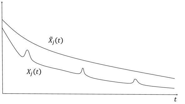
Figure 1: The behavior of $X_{j}(t)$ and $\tilde{X}_{j}(t)$. In the diagram it shows that $X_{j}(t)$ may grow at some time $t$, but it is bounded by its renormalized variable $\tilde{X}_{j}(t)$, which is always decaying.

1.2.5 Coupling Between Discrete Modes and Enhanced Damping Effect

The coupling between discrete modes also brings trouble in determining the exact decay rates. In the one simple eigenvalue case [25], it was proved that if $\frac{m}{2N+1}<\omega<\frac{m}{2N-1}$, then the discrete mode has a decay rate of $\langle t\rangle^{-\frac{1}{4N}}$, or equivalently $X\approx\langle t\rangle^{-\frac{1}{2N}}$. For the multiple eigenvalue case, by (1.14) we also have

$$\frac{d}{dt}\tilde{X}_{j}\lesssim-\tilde{X}_{j}^{2N_{j}+1},$$

which implies that $\tilde{X}_{j}\lesssim\langle t\rangle^{-\frac{1}{2N_{j}}}$. However, these decay rates of $\{\tilde{X}_{j}\}$ are not enough to close our estimates on $X$ and $f$. A new observation is that $\langle t\rangle^{-\frac{1}{2N_{j}}}$ may not be the optimal decay rate of $\tilde{X}_{j}.$ To illustrate, let us consider a two-states ODE model as an example:

$$\dot{X}_{1}=-3X_{1}^{3}-2X_{1}^{2}X_{2}-X_{1}X_{2}^{4},$$ (1.15)

$$\dot{X}_{2}=-5X_{2}^{5}-X_{1}^{2}X_{2}-4X_{1}X_{2}^{4}.$$ (1.16)

This is a toy model for a two-eigenvalue problem, with $\omega_{1}$ and $\omega_{2}$ satisfying the following conditions:

$$\frac{m}{3}<\omega_{1}<m,$$

$$\frac{m}{5}<\omega_{2}<\frac{m}{3},$$

$$2\omega_{1}+\omega_{2}>m,$$

$$\omega_{1}+2\omega_{2}<m.$$

If there is no coupling terms like $X_{1}^{2}X_{2}$ and $X_{1}X_{2}^{4}$ on the right hand side of (1.15) and (1.16), then we have $X_{1}\approx\langle t\rangle^{-\frac{1}{2}}$ and $X_{2}\approx\langle t\rangle^{-\frac{1}{4}}$. However, when the coupling between $X_{1}$ and $X_{2}$ exists, the situation can be better. Indeed, in (1.16) we see that the dominant term is still $-5X_{2}^{5}$, hence $X_{2}\approx\langle t\rangle^{-\frac{1}{4}}$ still holds. In (1.15), we have $X_{1}^{2}X_{2}\gg X_{1}^{3}$, thus $-2X_{1}^{2}X_{2}$ dominates $-3X_{1}^{3}$, which implies that $X_{1}$ decays at least at $\langle t\rangle^{-\frac{3}{4}}$!

This example shows that the interaction between discrete modes may accelerate the decay of some modes. In general cases, such enhanced damping effect could be much more involved, and the decay rate here is very sensitive to the size of each $\omega_{j}$ and the coefficients of resonant terms. We are not going to pursue how this mechanism would affect every single mode $\tilde{X}_{j}$, but turn to study the equation of every $\tilde{X}^{\lambda+\rho}$ for $(\lambda,\rho)\in\Lambda$, which is enough for our purpose. Indeed, by (1.14), we have (here we omit higher order terms for simplicity):

$$\frac{d}{dt}\tilde{X}^{\lambda+\rho}\lesssim-\sum_{1\leq j\leq n}\sum_{1\leq k\leq j}\sum_{(\tilde{\lambda},\tilde{\rho})\in\Lambda}\frac{\tilde{X}^{\lambda+\rho}\tilde{X}^{\tilde{\lambda}+\tilde{\rho}}}{\tilde{X}_{j}}(\lambda_{j}+\rho_{j})(\tilde{\lambda}_{k}+\tilde{\rho}_{k}).$$

Take $(\tilde{\lambda},\tilde{\rho})=(\lambda,\rho)$ and we get

$$\frac{d}{dt}\tilde{X}^{\lambda+\rho}\lesssim-\sum_{1\leq j\leq n}\frac{\tilde{X}^{2\lambda+2\rho}}{\tilde{X}_{j}}(\lambda_{j}+\rho_{j}).$$

This implies that

$$X^{\lambda+\rho}\lesssim\langle t\rangle^{-\frac{2N_{j}+1}{2N_{j}}},$$ (1.17)

for any $j$ with $\lambda_{j}+\rho_{j}\neq 0$. We remark that even the decay (1.17) may be not optimal, but it improves the following trivial estimate (for some $(\lambda,\rho)$)

$$X^{\lambda+\rho}\lesssim\langle t\rangle^{-\sum_{j}\frac{\lambda_{j}+\rho_{j}}{2N_{j}}},$$ (1.18)

which is the contribution of the enhanced damping effect. Actually, as in the two-eigenvalue problem, we have by (1.17) (choose $j=1$)

$$X_{1}^{2}X_{2}\lesssim\langle t\rangle^{-\frac{3}{2}},$$

while using (1.18) we only have

$$X_{1}^{2}X_{2}\lesssim\langle t\rangle^{-\frac{5}{4}}.$$

This improvement by the enhanced damping effect is crucial for our perturbation arguments and error estimates, see Theorem 7.1 for more details.

1.2.6 Error Estimates

A remaining technical difficulty is to estimate the error terms. As mentioned before, the exact decay rates of discrete modes are unattainable, thus we can not treat all higher order terms perturbatively. To address this issue, we need to explore the explicit structure of $\partial_{\bar{f}}\mathcal{R}$ and then use an iteration scheme to derive the following expansion of $f$:

$$f=\sum_{l=0}^{l_{0}-1}f^{(l)}_{M}+f^{(l_{0})}$$

for some large $l_{0}$, where

$$f^{(l)}_{M}\approx\sum_{(\mu,\nu)\in M^{(l)}}\bar{\xi}^{\mu}\xi^{\nu}\bar{Y}_{\mu\nu}^{(l)}.$$

This is achievable due to our refined normal form transformation mentioned in Section 1.2.1, see also Theorem 3.2. The virtue of this expansion is of two folds. First, the high order term $f^{(l)}_{M}(l\geq 1)$ enjoys the same form of resonance, thus its counterpart in the equation of $X_{j}$ can be controlled by

$$|X|\sum_{(\lambda,\rho)\in\Lambda^{*}}X^{\lambda+\rho}(\lambda_{j}+\rho_{j})+X_{j}\sum_{(\lambda,\rho)\in\Lambda^{*}}X^{\lambda+\rho}.$$

See Lemma 5.6. The first term can be controlled by the leading order term, while the second term can be absorbed by a uniformly bounded variable transformation, see (6.4).

Second, we mention that the Strichartz norms of every component of $f$ is bounded, which is crucial to prove the fast decay of $f^{(l_{0})}$ for sufficiently large $l_{0}$. To illustrate this, we write

$$B^{-1/2}f^{(l_{0})}= \int_{0}^{t}e^{-\mathrm{i}B(t-s)}\xi^{2}B^{-1/2}\left(\Psi B^{-1/2}f^{(l_{0})}\right)ds$$

$$-\mathrm{i}\int_{0}^{t}e^{-\mathrm{i}B(t-s)}B^{-1/2}\left(B^{-1/2}f^{(l_{0})}+B^{-1/2}\bar{f}^{(l_{0})}\right)^{3}ds+\cdots$$

where $\xi^{2}$ denotes some quadratic monomials of $\xi$ and $\bar{\xi}$ and we only list some typical terms for simplicity. The main difficulty of the estimate of $f^{(l_{0})}$ comes from the loss of derivatives. For example, if we choose to estimate the $L^{8}$ norm (or other $L^{p}$ norms for $p>6$), then by the classical dispersive estimates of the linear Klein-Gordon equation, we have

$$\|B^{-1/2}f^{(l_{0})}(t)\|_{W^{k,8}_{x}}\lesssim \int_{0}^{t}\langle t-s\rangle^{-\frac{9}{8}}\bigg{(}|\xi|^{2}\|B^{-1/2}f^{(l_{0})}(s)\|_{W^{k+1,8}_{x}}$$

$$+\|B^{-1/2}f^{(l_{0})}(t)\|_{W^{k+1,2}_{x}}^{\frac{4}{3}}\|B^{-1/2}f^{(l_{0})}(s)\|_{W^{k,8}_{x}}^{\frac{5}{3}}\bigg{)}ds+\cdots$$

Thus, we have to use $W^{k+1,8}_{x}$ norm of $B^{-1/2}f^{(l_{0})}$ to control its $W^{k,8}_{x}$ norm (for other $p>6$ the situation is similar), otherwise there is a loss of decay, see [25, 37]. To overcome this difficulty, we use a backward induction argument. By high order Strichartz estimates, we can prove that $\|B^{-1/2}f^{(l_{0})}(t)\|_{W^{k,8}_{x}}$ and $\|B^{-1/2}f^{(l_{0})}(t)\|_{W^{k,2}_{x}}$ are uniformly bounded for large $k$. Fix a large $k$, we then have

$$\|B^{-1/2}f^{(l_{0})}(t)\|_{W^{k-1,8}_{x}}\lesssim \int_{0}^{t}\langle t-s\rangle^{-\frac{9}{8}}\bigg{(}|\xi|^{2}\|B^{-1/2}f^{(l_{0})}(s)\|_{W^{k,8}_{x}}$$

$$+\|B^{-1/2}f^{(l_{0})}(t)\|_{W^{k,2}_{x}}^{\frac{4}{3}}\|B^{-1/2}f^{(l_{0})}(s)\|_{W^{k-1,8}_{x}}^{\frac{5}{3}}\bigg{)}ds+\cdots$$

$$\lesssim \int_{0}^{t}\langle t-s\rangle^{-\frac{9}{8}}\bigg{(}\langle s\rangle^{-\frac{1}{2N_{n}}}\|B^{-1/2}f^{(l_{0})}(s)\|_{W^{k,8}_{x}}$$

$$+\|B^{-1/2}f^{(l_{0})}(s)\|_{W^{k-1,8}_{x}}^{\frac{5}{3}}\bigg{)}ds+\cdots,$$

which implies that $\|B^{-1/2}f^{(l_{0})}(t)\|_{W^{k-1,8}_{x}}\lesssim\langle t\rangle^{-\frac{1}{2N_{n}}}$. Repeating this process, we can obtain

$$\|B^{-1/2}f^{(l_{0})}(t)\|_{W^{k-2,8}_{x}}\lesssim \int_{0}^{t}\langle t-s\rangle^{-\frac{9}{8}}\bigg{(}|\xi|^{2}\|B^{-1/2}f^{(l_{0})}(s)\|_{W^{k-1,8}_{x}}$$

$$+\|B^{-1/2}f^{(l_{0})}(t)\|_{W^{k-1,2}_{x}}^{\frac{4}{3}}\|B^{-1/2}f^{(l_{0})}(s)\|_{W^{k-2,8}_{x}}^{\frac{5}{3}}\bigg{)}ds+\cdots$$

$$\lesssim \int_{0}^{t}\langle t-s\rangle^{-\frac{9}{8}}\bigg{(}\langle s\rangle^{-\frac{1}{2N_{n}}}\|B^{-1/2}f^{(l_{0})}(s)\|_{W^{k-1,8}_{x}}$$

$$+\|B^{-1/2}f^{(l_{0})}(s)\|_{W^{k-2,8}_{x}}^{\frac{5}{3}}\bigg{)}ds+\cdots,$$

which implies that $\|B^{-1/2}f^{(l_{0})}(t)\|_{W^{k-2,8}_{x}}\lesssim\langle t\rangle^{-\frac{2}{2N_{n}}}$. In general, we can prove that for $k^{\prime}\leq\frac{9N_{n}}{4}$,

$$\|B^{-1/2}f^{(l_{0})}(t)\|_{W^{k-k^{\prime},8}_{x}}\lesssim\langle t\rangle^{-\frac{k^{\prime}}{2N_{n}}}.$$

Choose $k$ and $k^{\prime}$ large, we then get the desired decay estimate.

1.3 Structure of the Paper

The remaining part of this paper is organized as follows. In Section 2, we introduce some useful dispersive estimates and weighted inequalities for linear equations with potential. Besides, we present the global existence theory and energy conservation of the nonlinear Klein-Gordon equation. In Section 3, we begin our proof by performing Birkhoff normal form transformation. In Section 4, we use an iteration scheme to derive the expansion of $f$ up to higher orders. Then we isolate the key resonant terms in the dynamical equations of discrete modes and derive the generalized Fermi’s Golden Rule in Section 5. In Section 6, we introduce a new variable $\tilde{X}$ to cancel the bad resonances. In Section 7, we analyze the ODE and derive the asymptotic behavior of discrete modes. In Section 8, we give estimates of the continuum variable $f$ and error terms. In Section 9, we prove the main theorem in this paper.

1.4 Notations

Throughout our paper, we adopt the following notations.

• We write $A\lesssim B$ to mean that $A\leq CB$ for some absolute constant $C>0$. We use $A\approx B$ to denote both $A\lesssim B$ and $B\lesssim A.$

• We denote the vector $\xi=(\xi_{jk})_{1\leq j\leq n,1\leq k\leq l_{j}}\in\mathbb{C}^{\sum_{j}l_{j}}$. For multiple indexes $\mu=(\mu_{jk})_{1\leq j\leq n,1\leq k\leq l_{j}},\nu=(\nu_{jk})_{1\leq j\leq n,1\leq k\leq l_{j}}\in\mathbb{N}^{\sum_{j}l_{j}}$, we denote

  $$\xi^{\mu}=\prod_{j,k}\xi_{jk}^{\mu_{jk}},\quad\xi^{\mu}\bar{\xi}^{\nu}=\prod_{j,k}\xi_{jk}^{\mu_{jk}}\bar{\xi}_{jk}^{\nu_{jk}},\quad|\mu|=\sum_{jk}\mu_{jk}.$$

  Denote $\omega=(\omega_{jk})_{1\leq j\leq n,1\leq k\leq l_{j}},$ where $\omega_{jk}=\omega_{j}$. Hence,

  $$\omega\cdot\mu=\sum_{1\leq j\leq n}\sum_{1\leq k\leq l_{j}}\omega_{j}\mu_{jk}.$$

• We define the unit vector $e_{jk}\in\mathbb{Z}^{\sum_{j}l_{j}}$ such that it equals $1$ for the $jk$-th component and equals $0$ for other components.

• We define $\sum_{finite}$ to be a finite sum of terms with the same form, where we omit the summation index for simplicity.

2 Preliminaries: Linear Theory and Global Well-posedness

In this section, we provide some useful lemmas on the linear analysis for the Klein-Gordon equation with potential and the global well-posedness theory of the nonlinear Klein-Gordon equation (1.1).

2.1 Linear Dispersive Estimates

Consider the Cauchy problem for three dimensional linear Klein-Gordon equation with a potential

$$\begin{cases}\partial_{t}^{2}u-\Delta u+m^{2}u+V(x)u=0,&\quad t>0,x\in\mathbb{R}^{3},\\ u(0,x)=u_{0},\quad\partial_{t}u(0,x)=u_{1}.\end{cases}$$ (2.1)

Denote $B^{2}=-\Delta+m^{2}+V(x)$, then equation (2.1) can be solved as

$$u(t,x)=\cos{Bt}\ u_{0}+\frac{\sin Bt}{B}\ u_{1}.$$

For $V(x)=0$, i.e. free Klein-Gordon case, the standard $L^{p}$ dispersive estimates follow from an oscillatory integration method and the conservation of the $L^{2}$ norm. More precisely, the $L^{p}$ norm of the solution to $u(t,x)$ satisfies the dispersive decay estimate $\|u(t,\cdot)\|_{L^{p}}\leq C|t|^{-3(\frac{1}{2}-\frac{1}{p})}$.

For $V(x)\neq 0$, if $V(x)$ satisfies some suitable decay and regularity conditions, then the same decay rate of $u$ can be obtained by the $W^{k,p}$-boundedness of the wave operator after being projected on the continuous spectrum of $B$. For instance, see [17],[30],[42].

Lemma 2.1 ($L^{p}$ dispersive estimates).

Assume that $V(x)$ is a real-valued function and satisfies (V1),(V2). Let $1<p\leq 2$, $\frac{1}{p}+\frac{1}{p^{\prime}}=1$, $0\leq\theta\leq 1$, $l=0,1$, and $s=(4+\theta)(\frac{1}{2}-\frac{1}{p^{\prime}})$. Then

$$\|\mathrm{e}^{\mathrm{i}Bt}B^{-l}\mathbf{P}_{\mathrm{c}}\psi\|_{l,p^{\prime}}\lesssim|t|^{-(2+\theta)(\frac{1}{2}-\frac{1}{p^{\prime}})}\|\psi\|_{s,p},\quad|t|\geq 1,$$

and

$$\|\mathrm{e}^{\mathrm{i}Bt}B^{-l}\mathbf{P}_{\mathrm{c}}\psi\|_{l,p^{\prime}}\lesssim|t|^{-(2-\theta)(\frac{1}{2}-\frac{1}{p^{\prime}})}\|\psi\|_{s,p},\quad 0<|t|\leq 1.$$

Moreover, we also use the following Strichartz type estimates, see [3].

Lemma 2.2.

Assume (V1)-(V2). Then there exists a constant $C_{0}$ such that for any two admissible pairs $(p,q)$ and $(a,b)$ we have

$$\left\|e^{-\mathrm{i}tB}P_{c}u_{0}\right\|_{L_{t}^{p}W_{x}^{\frac{1}{q}-\frac{1}{p},q}}\leq C_{0}\left\|u_{0}\right\|_{W^{\frac{1}{2},2}}$$

$$\left\|\int_{0}^{t}e^{-\mathrm{i}(t-s)B}P_{c}F(s)ds\right\|_{L_{t}^{p}W_{x}^{\frac{1}{q}-\frac{1}{p},q}}\leq C_{0}\|F\|_{L_{t}^{a^{\prime}}W_{x}^{\frac{1}{a}-\frac{1}{b}+1,b^{\prime}}}.$$

Here an admissible pair $(p,q)$ means

$$\frac{2}{p}+\frac{3}{q}=\frac{3}{2},2\leq p\leq+\infty,6\geq q\geq 2.$$

Lemma 2.3.

Assume (V1)-(V2). Then for any $s>1$ there exists a constant $C_{0}=$ $C_{0}(s,a)$ such that for any admissible pair $(p,q)$ we have

$$\left\|\int_{0}^{t}e^{-\mathrm{i}(t-s)B}P_{c}F(s)ds\right\|_{L_{t}^{p}W_{x}^{\frac{1}{q}-\frac{1}{p},q}}\leq C_{0}\left\|B^{\frac{1}{2}}P_{c}F\right\|_{L_{t}^{a}L_{x}^{2,s}}$$

where for $p>2$ we can pick any $a\in[1,2]$ while for $p=2$ we pick $a\in[1,2)$.

2.2 Singular Resolvents and Time Decay

The following local decay estimates for singular resolvents $\mathrm{e}^{\mathrm{i}Bt}(B-\Lambda+\mathrm{i}0)^{-l}$, which was proved in [37], are also significant. Here, $\Lambda$ is a point in the interior of the continuous spectrum of $B(\Lambda>m)$.

Lemma 2.4 (Decay estimates for singular resolvents).

Assume that $V(x)$ is a real-valued function and satisfies (V1)-(V3). Let $\sigma>16/5$. Then for any point $\Lambda>m$ in the continuous spectrum of $B$, we have for $l=1,2:$

$$\left\|\langle x\rangle^{-\sigma}\mathrm{e}^{\mathrm{i}Bt}(B-\Lambda+\mathrm{i}0)^{-l}\mathbf{P}_{\mathrm{c}}\langle x\rangle^{-\sigma}\psi\right\|_{2}\lesssim\langle t\rangle^{-\frac{6}{5}}\|\psi\|_{1,2},\quad t>0,$$

$$\left\|\langle x\rangle^{-\sigma}\mathrm{e}^{\mathrm{i}Bt}(B-\Lambda-\mathrm{i}0)^{-l}\mathbf{P}_{\mathrm{c}}\langle x\rangle^{-\sigma}\psi\right\|_{2}\lesssim\langle t\rangle^{-\frac{6}{5}}\|\psi\|_{1,2},\quad t<0.$$

2.3 Global Well-Posedness and Energy Conservation

The global well-posedness of (1.1) with small initial data is well-known.

Theorem 2.5.

Assume $V\in L^{p}$ with $p>3/2$. Then, there exists $\varepsilon_{0}>0$ and $C>0$, such that for any $\left\|\left(u_{0},u_{1}\right)\right\|_{H^{1}\times L^{2}}\leq\epsilon<\varepsilon_{0}$, equation (1.1) admits exactly one solution $u\in C^{0}\left(\mathbb{R};H^{1}\right)\cap C^{1}\left(\mathbb{R};L^{2}\right)$ such that $(u(0),\partial_{t}u(0))=\left(u_{0},u_{1}\right)$. Furthermore, the map $\left(u_{0},u_{1}\right)\mapsto(u(t),\partial_{t}u(t))$ is continuous from the ball $\left\|\left(u_{0},u_{1}\right)\right\|_{H^{1}\times L^{2}}<\varepsilon_{0}$ to $C^{0}\left(I;H^{1}\right)\times C^{0}\left(I;L^{2}\right)$ for any bounded interval $I$. Moreover, the energy

$$\mathcal{E}[u,\partial_{t}u]\equiv\frac{1}{2}\int(\partial_{t}u)^{2}+|\nabla u|^{2}+m^{2}u^{2}+V(x)u^{2}dx-\frac{\lambda}{4}\int u^{4}dx.$$

is conserved and

$$\|(u(t),v(t))\|_{H^{1}\times L^{2}}\leq C\left\|\left(u_{0},v_{0}\right)\right\|_{H^{1}\times L^{2}}.$$

We refer to [6] for details.

3 Normal Form Transformation

In this section, we present a new Birkhoff normal form transformation which is a refined version of Theorem 4.9 in [3].

3.1 Hamiltonian Structure

Recall the 3D nonlinear Klein Gordon equation (NLKG)

$$u_{tt}-\Delta u+Vu+m^{2}u=u^{3},\quad(t,x)\in\mathbb{R}\times\mathbb{R}^{3},$$ (3.1)

which is an Hamiltonian perturbation of the linear Klein-Gordon equation with potential. More precisely, in $H^{1}\left(\mathbb{R}^{3},\mathbb{R}\right)\times L^{2}\left(\mathbb{R}^{3},\mathbb{R}\right)$ endowed with the standard symplectic form, namely

$$\Omega\left(\left(u_{1},v_{1}\right);\left(u_{2},v_{2}\right)\right):=\left\langle u_{1},v_{2}\right\rangle_{L^{2}}-\left\langle u_{2},v_{1}\right\rangle_{L^{2}},$$

we consider the Hamiltonian

$$H =H_{L}+H_{P},$$

$$H_{L} :=\int_{\mathbb{R}^{3}}\frac{1}{2}\left(v^{2}+|\nabla u|^{2}+Vu^{2}+m^{2}u^{2}\right)dx,$$

$$H_{P} :=\int_{\mathbb{R}^{3}}-\frac{1}{4}u^{4}dx.$$

The corresponding Hamilton equations are $\dot{v}=-\nabla_{u}H,\dot{u}=\nabla_{v}H$, where $\nabla_{u}H$ is the gradient with respect to the $L^{2}$ metric, explicitly defined by

$$\left\langle\nabla_{u}H(u),h\right\rangle=d_{u}H(u)h,\quad\forall h\in H^{1},$$

and $d_{u}H(u)$ is the Frechét derivative of $H$ with respect to $u$. It is easy to see that the Hamilton equations are explicitly given by

$$\left(\dot{v}=\Delta u-Vu-m^{2}u+u^{3},\dot{u}=v\right)\Longleftrightarrow\ddot{u}=\Delta u-Vu-m^{2}u+u^{3}.$$

Write

$$u=\sum_{j=1}^{n}\sum_{k=1}^{l_{j}}q_{jk}\varphi_{jk}+P_{c}u,\quad v=\sum_{j=1}^{n}\sum_{k=1}^{l_{j}}p_{jk}\varphi_{jk}+P_{c}v,$$

with a slightly abuse of notations, from now on we denote

$$B:=P_{c}\left(-\Delta+V+m^{2}\right)^{1/2}P_{c},$$

and define the complex variables

$$\xi_{jk}:=\frac{q_{jk}\sqrt{\omega_{j}}+\mathrm{i}\frac{p_{jk}}{\sqrt{\omega_{j}}}}{\sqrt{2}},\quad f:=\frac{B^{1/2}P_{c}u+\mathrm{i}B^{-1/2}P_{c}v}{\sqrt{2}}.$$ (3.2)

Then, in terms of these variables the symplectic form can be written as

$$\begin{array}[]{r}\Omega\left(\left(\xi^{(1)},f^{(1)}\right);\left(\xi^{(2)},f^{(2)}\right)\right)=2\operatorname{Re}\left[\mathrm{i}\left(\xi^{(1)}\cdot\bar{\xi}^{(2)}+\left\langle f^{(1)},\bar{f}^{(2)}\right\rangle\right)\right]\\ =-\mathrm{i}\sum_{j}\left(\bar{\xi}^{(1)}\cdot\xi^{(2)}-\xi^{(1)}\cdot\bar{\xi}^{(2)}\right)-\mathrm{i}\left(\left\langle f^{(2)},\bar{f}^{(1)}\right\rangle-\left\langle f^{(1)},\bar{f}^{(2)}\right\rangle\right)\end{array}$$

and the Hamilton equations take the form

$$\dot{\xi}_{jk}=-\mathrm{i}\frac{\partial H}{\partial\bar{\xi}_{jk}},\quad\dot{f}=-\mathrm{i}\nabla_{\bar{f}}H.$$

where

$$\begin{gathered}H_{L}=\sum_{j,k}\omega_{j}\left|\xi_{jk}\right|^{2}+\langle\bar{f},Bf\rangle,\\ H_{P}(\xi,f)=-\frac{1}{4}\int_{\mathbb{R}^{3}}\left(\sum_{j,k}\frac{\xi_{jk}+\bar{\xi}_{jk}}{\sqrt{2\omega_{j}}}\varphi(x)+U(x)\right)^{4}dx\end{gathered}$$

with $U=B^{-\frac{1}{2}}(f+\bar{f})/\sqrt{2}\equiv P_{c}u$. The Hamiltonian vector field $X_{H}$ of a function is given by

$$X_{H}(\xi,\bar{\xi},f,\bar{f})=\left(-\mathrm{i}\frac{\partial H}{\partial\bar{\xi}},\mathrm{i}\frac{\partial H}{\partial\xi},-\mathrm{i}\nabla_{\bar{f}}H,\mathrm{i}\nabla_{f}H\right).$$

The associate Poisson bracket is given by

$$\{H,K\}:= \mathrm{i}\left(\frac{\partial H}{\partial\xi}\cdot\frac{\partial K}{\partial\bar{\xi}}-\frac{\partial H}{\partial\bar{\xi}}\cdot\frac{\partial K}{\partial\xi}\right)$$

$$+\mathrm{i}\left\langle\nabla_{f}H,\nabla_{\bar{f}}K\right\rangle-\mathrm{i}\left\langle\nabla_{\bar{f}}H,\nabla_{f}K\right\rangle.$$

Denote $z=(\xi,f),\mathbf{f}=(f,\bar{f}),$ and $\mathcal{P}^{k,s}=\mathbb{C}^{\sum_{j}l_{j}}\times P_{c}H^{k,s}\left(\mathbb{R}^{3},\mathbb{C}\right)$, where

$$H^{k,s}\left(\mathbb{R}^{3},\mathbb{C}\right)=\left\{f:\mathbb{R}^{3}\rightarrow\mathbb{C}\text{ s.t. }\|f\|_{H^{s,k}}:=\left\|\langle x\rangle^{s}(-\Delta+1)^{k/2}f\right\|_{L^{2}}<\infty\right\}.$$

3.2 Normal Form Transformation

Definition 3.1 (Normal Form).

A polynomial $Z$ is in normal form if

$$Z=Z_{0}+Z_{1}$$

where $Z_{0}$ is a linear combination of monomials $\xi^{\mu}\overline{\xi^{\nu}}$ such that $\omega\cdot(\mu-\nu)=0$ , and $Z_{1}$ is a linear combination of monomials of the form

$$\xi^{\mu}\bar{\xi}^{\nu}\int\Phi(x)f(x)dx,\quad\bar{\xi}^{\mu}\xi^{\nu}\int\Phi(x)\bar{f}(x)dx$$

with indexes satisfying

$$\omega\cdot(\nu-\mu)>m,$$

and $\Phi\in\mathcal{S}\left(\mathbb{R}^{3},\mathbb{C}\right).$

Now we present the following normal form transformation.

Theorem 3.2.

For any $\kappa>0,s>0$ and any integer $r\geq 0$, there exist open neighborhoods of the origin $\mathcal{U}_{r,\kappa,s}\subset\mathcal{P}^{1/2,0}$, $\mathcal{U}_{r}^{-\kappa,-s}\subset\mathcal{P}^{-\kappa,-s}$, and an analytic canonical transformation $\mathcal{T}_{r}:\mathcal{U}_{r,\kappa,s}\rightarrow\mathcal{P}^{1/2,0}$, such that $\mathcal{T}_{r}$ puts the system in normal form up to order $2r+4$. More precisely, we have

$$H^{(r)}:=H\circ\mathcal{T}_{r}=H_{L}+Z^{(r)}+\mathcal{R}^{(r)}$$

where: (i) $Z^{(r)}\in\mathbb{R}$ is a polynomial of degree $2r+2$ which is in normal form,
(ii) $I-\mathcal{T}_{r}$ extends into an analytic map from $\mathcal{U}_{r}^{-\kappa,-s}$ to $\mathcal{P}^{\kappa,s}$ and

$$\left\|z-\mathcal{T}_{r}(z)\right\|_{\mathcal{P}^{\kappa,s}}\lesssim\|z\|_{\mathcal{P}^{-\kappa,-s}}^{3}.$$ (3.3)

(iii) we have $\mathcal{R}^{(r)}=\sum_{d=0}^{5}\mathcal{R}_{d}^{(r)}$ with the following properties:
(iii.0) we have

$$\mathcal{R}_{0}^{(r)}=\sum_{|\mu+\nu|=2r+4}a_{\mu\nu}^{(r)}\left(\xi\right)\xi^{\mu}\bar{\xi}^{\nu}$$

where $a_{\mu\nu}^{(r)}\in C^{\infty},\overline{a_{\mu\nu}^{(r)}}=a_{\nu\mu}^{(r)}$ satisfying the following expansion with a sufficiently large integer $M^{\star}>0$:

$$a_{\mu\nu}^{(r)}(\xi)=\sum_{k=0}^{M^{\star}}\sum_{|\alpha+\beta|=2k}a^{(r)}_{\mu\nu\alpha\beta}\xi^{\alpha}\bar{\xi}^{\beta},$$ (3.4)

(iii.1) we have

$$\mathcal{R}_{1}^{(r)}=\sum_{|\mu+\nu|=2r+3}\xi^{\mu}\bar{\xi}^{\nu}\int_{\mathbb{R}^{3}}\mathbf{\Phi}_{\mu\nu}^{(r)}\left(x,\xi\right)\cdot\mathbf{f}(x)dx$$

where $\mathbf{\Phi}_{\mu\nu}^{(r)}=(\Phi_{\mu\nu}^{(r)},\overline{\Phi_{\nu\mu}^{(r)}})$ is smooth and satisfies the following expansion:

$$\Phi_{\mu\nu}^{(r)}(\cdot,\xi)=\sum_{k=0}^{M^{\star}}\sum_{|\alpha+\beta|=2k}\Phi^{(r)}_{\mu\nu\alpha\beta}(x)\xi^{\alpha}\bar{\xi}^{\beta}$$ (3.5)

with $\Phi^{(r)}_{\mu\nu\alpha\beta}(x)\in\mathcal{S}\left(\mathbb{R}^{3},\mathbb{C}\right)$.
(iii.2-4) for $d=2,3,4$, we have

$$\mathcal{R}_{d}^{(r)}=\int_{\mathbb{R}^{3}}F_{d}^{(r)}\left(x,z\right)[U(x)]^{d}dx+\sum_{finite}\prod_{l=1}^{d}\int_{\mathbb{R}^{3}}\mathbf{\Lambda}_{dl}^{(r)}(x,z)\cdot\mathbf{f}dx,$$ (3.6)

where $F_{4}^{(r)}\equiv 1;$ for $d=2,3,$ $F_{d}^{(r)}(x,z)\in\mathbb{R}$ is a linear combination of terms of the form

$$\sum_{k=0}^{M^{\star}}\sum_{i=0}^{k}\sum_{|\mu+\nu|=4-d+2k-i}\xi^{\mu}\bar{\xi}^{\nu}\prod_{j=1}^{i}\int\mathbf{\Phi}^{ij}_{\mu\nu}(x)\cdot\mathbf{f}dx\Psi^{i}_{\mu\nu}(x),$$ (3.7)

and $\mathbf{\Lambda}_{dl}^{(r)}(x,z)=(\Lambda_{dl}^{(r)},\overline{\Lambda_{dl}^{(r)}})\ (d=2,3,4)$, $\Lambda_{dl}^{(r)}$ is a linear combination of terms of the form

$$\sum_{k=0}^{M^{\star}}\sum_{i=0}^{k}\sum_{|\mu+\nu|=1+2k-i}\xi^{\mu}\bar{\xi}^{\nu}\prod_{j=1}^{i}\int\tilde{\mathbf{\Phi}}^{ij}_{\mu\nu}(x)\cdot\mathbf{f}dx\tilde{\Psi}^{i}_{\mu\nu}(x),$$ (3.8)

with $\mathbf{\Phi}^{ij}_{\mu\nu}(x),\tilde{\mathbf{\Phi}}^{ij}_{\mu\nu}(x)\in\left(\mathcal{S}\left(\mathbb{R}^{3},\mathbb{C}\right)\right)^{2},\Psi^{i}_{\mu\nu}(x),\tilde{\Psi}^{i}_{\mu\nu}(x)\in\mathcal{S}\left(\mathbb{R}^{3},\mathbb{C}\right),$.
(iii.5) for $d=5$, we have

$$\left\|\nabla_{z,\bar{z}}\mathcal{R}_{5}^{(r)}\right\|_{\left(\mathcal{P}^{\kappa,s}\right)^{2}}\lesssim|\xi|^{M^{\star}}.$$

Remark 3.3.

Here the constant $M^{\star}$ is chosen to be sufficiently large, for our paper $M^{\star}=100N_{n}$ is sufficient.

Proof.

The proof is similar to Theorem 3.3 in [25], we shall give a sketch here for self-completeness. We prove Theorem 3.2 by induction. With some slightly abuses of notations, we denote $a$ with indexes as a constant, and $\Phi$ or $\Psi$ with indexes as a Schwartz function; they may change line from line, depending on the context.
(Step 0) First, when $r=0$, Theorem 3.2 holds with $\mathcal{T}_{0}=I,Z^{(0)}=0,\mathcal{R}^{(0)}=H_{P}.$
(Step $r\to r+1$) Now we assume that the theorem holds for some $r\geq 0$, we shall prove this for $r+1$. More precisely, define

$$\mathcal{R}_{02}^{(r)}=\mathcal{R}_{0}^{(r)}-\sum_{|\mu+\nu|=2r+4}a_{\mu\nu}^{(r)}(0)\xi^{\mu}\bar{\xi}^{\nu},$$

$$\mathcal{R}_{12}^{(r)}=\mathcal{R}_{1}^{(r)}-\sum_{|\mu+\nu|=2r+3}\xi^{\mu}\bar{\xi}^{\nu}\int_{\mathbb{R}^{3}}\mathbf{\Phi}_{\mu\nu}^{(r)}(x,0)\cdot\mathbf{f}(x)dx.$$

By (3.4) and (3.5), we have

$$\mathcal{R}_{02}^{(r)}+\mathcal{R}_{12}^{(r)}= \sum_{|\mu+\nu|=2r+6}a_{\mu\nu}^{(r+1)}(\xi)\xi^{\mu}\bar{\xi}^{\nu}$$

$$+\sum_{|\mu+\nu|=2r+5}\xi^{\mu}\bar{\xi}^{\nu}\int_{\mathbb{R}^{3}}\mathbf{\Phi}_{\mu\nu}^{(r+1)}(x,\xi)\cdot\mathbf{f}(x)dx$$

where the coefficients $a_{\mu\nu}^{(r+1)}(\xi),\mathbf{\Phi}_{\mu\nu}^{(r+1)}(x,\xi)$ satisfy (3.4)-(3.5) respectively, with $r$ replaced by $r+1$.

Set

$$K_{r+1}:= \sum_{|\mu+\nu|=2r+4}a_{\mu\nu}^{(r)}(0)\xi^{\mu}\bar{\xi}^{\nu}+\sum_{|\mu+\nu|=2r+3}\xi^{\mu}\bar{\xi}^{\nu}\int_{\mathbb{R}^{3}}\mathbf{\Phi}_{\mu\nu}^{(r)}(x,0)\cdot\mathbf{f}(x)d,$$

which is real valued. Then, we solve the following homological equation

$$\left\{H_{L},\chi_{r+1}\right\}+Z_{r+1}=K_{r+1},$$

with $Z_{r+1}$ in normal form. Thus,

$$Z_{r+1}= \sum_{\begin{subarray}{c}|\mu+\nu|=2r+4\\ \omega\cdot(\mu-\nu)=0\end{subarray}}a_{\mu\nu}^{(r)}(0)\xi^{\mu}\bar{\xi}^{\nu}+\sum_{\begin{subarray}{c}|\mu+\nu|=2r+3\\ \omega\cdot(\mu-\nu)<-m\end{subarray}}\xi^{\mu}\bar{\xi}^{\nu}\int\Phi_{\mu\nu}^{(r)}(x,0)f(x)dx$$

$$+\sum_{\begin{subarray}{c}|\mu+\nu|=2r+3\\ \omega\cdot(\mu-\nu)>m\end{subarray}}\xi^{\mu}\bar{\xi}^{\nu}\int\overline{\Phi_{\nu\mu}^{(r)}}(x,0)\bar{f}(x)dx,$$

and

$$\chi_{r+1}= i\sum_{\begin{subarray}{c}|\mu+\nu|=2r+4\\ \omega\cdot(\mu-\nu)\neq 0\end{subarray}}\frac{a_{\mu\nu}^{(r)}(0)}{\omega\cdot(\mu-\nu)}\xi^{\mu}\bar{\xi}^{\nu}+i\sum_{\begin{subarray}{c}|\mu+\nu|=2r+3\\ \omega\cdot(\mu-\nu)>-m\end{subarray}}\xi^{\mu}\bar{\xi}^{\nu}\int R_{\nu\mu}\Phi_{\mu\nu}^{(r)}(x,0)fdx$$

$$-i\sum_{\begin{subarray}{c}|\mu+\nu|=2r+3\\ \omega\cdot(\mu-\nu)<m\end{subarray}}\xi^{\mu}\bar{\xi}^{\nu}\int R_{\mu\nu}\overline{\Phi_{\nu\mu}^{(r)}}(x,0)\bar{f}dx,$$

where the operator

$$R_{\mu\nu}:=(B-\omega\cdot(\mu-\nu))^{-1}.$$

Let $\phi_{r+1}$ be the Lie transform generated by $\chi_{r+1}$, i.e. $\phi_{r+1}=\phi_{r+1}^{t}|_{t=1}$, where

$$\frac{d\phi_{r+1}^{t}}{dt}=X_{\chi_{r+1}}=(-i\partial_{\bar{\xi}}\chi_{r+1},-i\nabla_{\bar{f}}\chi_{r+1}).$$

Then, for $z^{\prime}=(\xi^{\prime},f^{\prime})=\phi_{r+1}(\xi,f),$ we have following expansion, see Lemma 3.1 in [25]:

$$\xi^{\prime}_{jk}=\xi_{jk}+\sum_{l=1}^{\infty}\sum_{i=0}^{l}\sum_{|\mu+\nu|=(2r+2)l+1-i}a_{jk,i\mu\nu}\xi^{\mu}\bar{\xi}^{\nu}\sum_{finite}\prod_{\alpha=1}^{i}\int\mathbf{\Phi}_{\alpha\mu\nu}^{jk,i}\cdot\mathbf{f}dx,$$ (3.9)

$$f^{\prime}=f+\sum_{l=1}^{\infty}\sum_{i=0}^{l-1}\sum_{|\mu+\nu|=(2r+2)l+1-i}\xi^{\mu}\bar{\xi}^{\nu}\sum_{finite}\prod_{\alpha=1}^{i}\int\mathbf{\Lambda}_{\alpha\mu\nu}^{i}\cdot\mathbf{f}dx\Psi_{\mu\nu}^{i}.$$ (3.10)

Recall that

$$R^{(r)}=K_{r+1}+R^{(r)}_{02}+R^{(r)}_{12}+\sum_{d=2}^{5}R^{(r)}_{d},$$

and $K_{r+1}=Z_{r+1}+\{H_{L},\chi_{r+1}\}$, we have

$$H^{(r+1)}\triangleq H^{(r)}\circ\phi_{r+1}=H\circ(\mathcal{T}_{r}\circ\phi_{r+1})\equiv H\circ\mathcal{T}_{r+1}$$

$$= H_{L}\circ\phi_{r+1}+Z^{(r)}\circ\phi_{r+1}+R^{(r)}\circ\phi_{r+1}$$

$$= H_{L}+Z^{(r)}+Z_{r+1}$$

$$+[H_{L}\circ\phi_{r+1}-(H_{L}+\{\chi_{r+1},H_{L}\})]$$ (3.11)

$$+Z^{(r)}\circ\phi_{r+1}-Z^{(r)}$$ (3.12)

$$+(K_{r+1}\circ\phi_{r+1}-K_{r+1})$$ (3.13)

$$+(R^{(r)}_{02}+R^{(r)}_{12})\circ\phi_{r+1}$$ (3.14)

$$+\sum_{d=2}^{5}R^{(r)}_{d}\circ\phi_{r+1}.$$ (3.15)

We define $Z^{(r+1)}=Z^{(r)}+Z_{r+1}$ in the normal form of order $2r+4$. For the term (3.11), we have

$$H_{L}\circ\phi_{r+1}-(H_{L}+\{\chi_{r+1},H_{L}\})$$

$$= \sum_{k=2}^{\infty}\frac{1}{k!}\underbrace{\{\chi_{r+1},\dots\{\chi_{r+1}}_{k\text{ times}},H_{L}\}\}$$

$$= \sum_{k=2}^{\infty}\sum_{i=0}^{k}\sum_{|\mu+\nu|=2(r+1)k+2-i}a_{i\mu\nu}\xi^{\mu}\bar{\xi}^{\nu}\sum_{finite}\prod_{j=1}^{i}\int\mathbf{\Phi}_{\mu\nu}^{ij}\cdot\mathbf{f}dx$$

$$= \sum_{k=2}^{M^{*}}\left(\sum_{|\mu+\nu|=2(r+1)k+2}a_{0\mu\nu}\xi^{\mu}\bar{\xi}^{\nu}+\sum_{|\mu+\nu|=2(r+1)k+1}a_{1\mu\nu}\xi^{\mu}\bar{\xi}^{\nu}\int\mathbf{\Phi}^{11}_{\mu\nu}\cdot\mathbf{f}dx\right)$$

$$+\sum_{k=2}^{M^{*}}\sum_{i=2}^{k}\sum_{|\mu+\nu|=2(r+1)k+2-i}a_{i\mu\nu}\xi^{\mu}\bar{\xi}^{\nu}\sum_{finite}\prod_{j=1}^{i}\int\mathbf{\Phi}_{\mu\nu}^{ij}\cdot\mathbf{f}dx+\mathcal{O}(|\xi|^{M^{*}}).$$

Thus (3.11) can be absorbed into $R^{(r+1)}_{0},R^{(r+1)}_{1}$, $R^{(r+1)}_{2}$ and $R^{(r+1)}_{5}$.

The terms (3.12), (3.13) and (3.14) can be handled similarly.

For the term (3.15), denote $f^{\prime}=f+G_{f},U^{\prime}=U+G_{U}$, then for $d=2,3,4$, we have

$$R^{(r)}_{d}\circ\phi_{r+1}$$

$$= \int_{\mathbb{R}^{3}}F_{d}^{(r)}\left(x,z^{\prime}\right)(U+G_{U})^{d}dx+\sum_{finite}\prod_{l=1}^{d}\int_{\mathbb{R}^{3}}\mathbf{\Lambda}_{dl}^{(r)}(x,z^{\prime})\cdot\left(\mathbf{f}+\mathbf{G}_{f}\right)dx$$

$$= \sum_{j=0}^{d}\left[\int F_{d}^{(r)}\left(x,z^{\prime}\right)U^{j}G_{U}^{d-j}dx+\sum_{finite}\sum_{l_{i}}\prod_{i=1}^{j}\int_{\mathbb{R}^{3}}\mathbf{\Lambda}_{d,l_{i}}^{(r)}(x,z^{\prime})\cdot\mathbf{f}dx\prod_{l\neq l_{i}}\int_{\mathbb{R}^{3}}\mathbf{\Lambda}_{dl}^{(r)}(x,z^{\prime})\cdot\mathbf{G}_{f}dx\right]$$

$$:= \sum_{j=0}^{d}H_{dj}.$$

By (3.10), we have

$$G_{f}=\sum_{k=1}^{\infty}\sum_{i=0}^{k-1}\sum_{|\mu+\nu|=(2r+2)k+1-i}\xi^{\mu}\bar{\xi}^{\nu}\sum_{finite}\prod_{j=1}^{i}\int\mathbf{\Lambda}_{\mu\nu}^{ij}\cdot\mathbf{f}dx\Psi_{\mu,\nu}^{i},\quad G_{U}=(G_{f}+\overline{G_{f}})/\sqrt{2B}.$$

Therefore, by (3.7), (3.8) and (3.9), we derive

$$H_{d0} =\int F_{d}^{(r)}\left(x,z^{\prime}\right)G_{U}^{d}dx+\sum_{finite}\prod_{l=1}^{d}\int_{\mathbb{R}^{3}}\mathbf{\Lambda}_{dl}^{(r)}(x,z^{\prime})\cdot\mathbf{G}_{f}dx$$

$$=\sum_{k=0}^{M^{*}}\sum_{i=0}^{k}\sum_{|\mu+\nu|=4+(2r+2)d+2k-i}a_{i\mu\nu}\xi^{\mu}\bar{\xi}^{\nu}\sum_{finite}\prod_{j=1}^{i}\int\mathbf{\Phi}_{\mu\nu}^{ij}\cdot\mathbf{f}dx+\mathcal{O}(|\xi|^{M^{*}}),$$

$$H_{d1} =\int F_{d}^{(r)}\left(x,z^{\prime}\right)UG_{U}^{d-1}dx+\sum_{finite}\sum_{i=1}^{d}\int_{\mathbb{R}^{3}}\mathbf{\Lambda}_{di}^{(r)}(x,z^{\prime})\cdot\mathbf{f}dx\prod_{l\neq i}\int_{\mathbb{R}^{3}}\mathbf{\Lambda}_{dl}^{(r)}(x,z^{\prime})\cdot\mathbf{G}_{f}dx$$

$$=\sum_{k=0}^{M^{*}}\sum_{i=0}^{k}\sum_{|\mu+\nu|=3+(2r+2)(d-1)+2k-i}a_{i\mu\nu}\xi^{\mu}\bar{\xi}^{\nu}\sum_{finite}\prod_{j=1}^{i+1}\int\mathbf{\Phi}_{\mu\nu}^{ij}\cdot\mathbf{f}dx+\mathcal{O}(|\xi|^{M^{*}}),$$

and for $2\leq j\leq d$,

$$H_{dj} =\int F_{d}^{(r)}\left(x,z^{\prime}\right)U^{j}G_{U}^{d-j}dx+\sum_{finite}\sum_{l_{i}}\prod_{i=1}^{j}\int_{\mathbb{R}^{3}}\mathbf{\Lambda}_{d,l_{i}}^{(r)}(x,z^{\prime})\cdot\mathbf{f}dx\prod_{l\neq l_{i}}\int_{\mathbb{R}^{3}}\mathbf{\Lambda}_{dl}^{(r)}(x,z^{\prime})\cdot\mathbf{G}_{f}dx$$

$$=\int_{\mathbb{R}^{3}}F_{j}^{(r+1)}\left(x,z\right)U^{j}dx+\sum_{finite}\prod_{l=1}^{j}\int_{\mathbb{R}^{3}}\mathbf{\Lambda}_{jl}^{(r+1)}(x,z)\cdot\mathbf{f}dx+\mathcal{O}(|\xi|^{M^{*}})$$

where

$$F_{j}^{(r+1)} =F_{d}^{(r)}\left(x,z^{\prime}\right)G_{U}^{d-j}-\mathcal{O}(|\xi|^{M^{*}})$$

$$=\sum_{k=0}^{M^{*}}\sum_{i=0}^{k}\sum_{|\mu+\nu|=4-j+(2r+2)(d-j)+2k-i}a_{i\mu\nu}\xi^{\mu}\bar{\xi}^{\nu}\sum_{finite}\prod_{l=1}^{i}\int\mathbf{\Phi}_{\mu\nu}^{il}\cdot\mathbf{f}dx\psi^{l}_{\mu\nu}(x),$$

note that $F_{4}^{(r+1)}\equiv 1.$ Thus $H_{dj}$ can be absorbed into $R^{(r+1)}$. Finally, it is direct to see $R^{(r)}_{5}\circ\phi_{r+1}$ can be absorbed into $R^{(r+1)}_{5}.$ ∎

4 Decoupling of Discrete and Continuum Modes: An Iteration Process

Applying Theorem 3.2 for $r=100N_{n}$, we obtain a new Hamiltonian

$$H=H_{L}(\xi,\mathbf{f})+Z_{0}(\xi)+Z_{1}(\xi,\mathbf{f})+\mathcal{R},$$

where

$$Z_{1}(\xi,\mathbf{f}):=\langle G,f\rangle+\langle\bar{G},\bar{f}\rangle,$$

$$G:=\sum_{(\mu,\nu)\in M}\xi^{\mu}\bar{\xi}^{\nu}\Phi_{\mu\nu}(x),\Phi_{\mu\nu}\in\mathcal{S}\left(\mathbb{R}^{3},\mathbb{C}\right),$$

with

$$M=\{(\mu,\nu)\mid|\mu+\nu|=2k+1,0\leq k\leq 100N_{n},\omega\cdot(\nu-\mu)>m\}.$$

Then, the corresponding Hamilton equations are

$$\dot{f} =-\mathrm{i}(Bf+\bar{G})-\mathrm{i}\partial_{\bar{f}}\mathcal{R},$$ (4.1)

$$\dot{\xi}_{jk} =-\mathrm{i}\omega_{j}\xi_{jk}-\mathrm{i}\partial_{\bar{\xi}_{jk}}Z_{0}-\mathrm{i}\left\langle\partial_{\bar{\xi}_{jk}}G,f\right\rangle-\mathrm{i}\left\langle\partial_{\bar{\xi}_{jk}}\bar{G},\bar{f}\right\rangle-\mathrm{i}\partial_{\bar{\xi}_{jk}}\mathcal{R}.$$ (4.2)

4.1 Structure of The Error Term $\partial_{\bar{f}}\mathcal{R}$

In [25], it is sufficient to treat $\partial_{\bar{f}}\mathcal{R}$ as an error term. However, for the multiple eigenvalues case, to get finer estimates of every $\xi_{jk}$, we have to explore an explicit structure of $\partial_{\bar{f}}\mathcal{R}$ . By Theorem 3.2, we have

Proposition 4.1.

$\partial_{\bar{f}}\mathcal{R}=\sum_{d=1}^{5}\partial_{\bar{f}}\mathcal{R}_{d}$ satisfies following properties:
(i) $\partial_{\bar{f}}\mathcal{R}_{1}$ is a linear combination of terms $\xi^{\mu}\bar{\xi}^{\nu}\Psi$, where $|\mu+\nu|\geq 100N,\Psi$ is smooth.
(ii-iii) For $2\leq d\leq 3$, $\partial_{\bar{f}}\mathcal{R}_{d}$ are linear combinations of terms of following forms

$$\xi^{\mu}\bar{\xi}^{\nu}\prod_{j}^{i}\int\mathbf{\Phi}_{j}\cdot\mathbf{f}dx\int\Psi U^{d}dx\Psi^{\prime},\quad|\mu+\nu|=5-d+2k-i,0\leq i\leq k,$$

$$\xi^{\mu}\bar{\xi}^{\nu}\prod_{j}^{i}\int\mathbf{\Phi}_{j}\cdot\mathbf{f}dxB^{-1/2}\left(\Psi U^{d-1}\right),\quad|\mu+\nu|=4-d+2k-i,0\leq i\leq k,$$

$$\xi^{\mu}\bar{\xi}^{\nu}\prod_{j}^{d-1+i}\int\mathbf{\Phi}_{j}\cdot\mathbf{f}dx\Psi,\quad|\mu+\nu|=4-d+2k-i,0\leq i\leq k.$$

(iv) $\partial_{\bar{f}}\mathcal{R}_{4}$ is a linear combination of terms of following forms

$$B^{-1/2}\left(\Psi U^{3}\right)$$

$$\xi^{\mu}\bar{\xi}^{\nu}\prod_{j}^{3+i}\int\mathbf{\Phi}_{j}\cdot\mathbf{f}dx\Psi,\quad|\mu+\nu|=2k-i,0\leq i\leq k.$$

(v) $\|\partial_{\bar{f}}\mathcal{R}_{5}\|_{H^{s,k}}\lesssim|\xi|^{M^{*}}$ for any $s,k$.

Rearranging these components, we can write

$$\partial_{\bar{f}}\mathcal{R}=\sum_{d=0}^{4}Q_{d}(\xi,\bar{\xi},f,\bar{f}),$$

where $\|Q_{0}\|_{H^{s,k}}\lesssim|\xi|^{100N},$ $Q_{1}(\xi,\bar{\xi},f,\bar{f})$ is a linear combination of terms in the form of

$$\xi^{\mu}\bar{\xi}^{\nu}B^{-1/2}\left(\Psi U\right),\ \xi^{\mu}\bar{\xi}^{\nu}\int\mathbf{\Phi}\cdot\mathbf{f}dx\Psi,\quad|\mu+\nu|=2+2k,k\geq 0.$$

$Q_{2}(\xi,\bar{\xi},f,\bar{f})$ a linear combination of terms in the form of

$$\xi^{\mu}\bar{\xi}^{\nu}\int\Psi U^{2}dx\Psi^{\prime},\quad|\mu+\nu|=3+2k,k\geq 0,$$

$$\xi^{\mu}\bar{\xi}^{\nu}B^{-1/2}\left(\Psi U^{2}\right),\quad|\mu+\nu|=1+2k,k\geq 0,$$

$$\xi^{\mu}\bar{\xi}^{\nu}\prod_{j=1}^{2}\int\mathbf{\Phi}_{j}\cdot\mathbf{f}dx\Psi,\quad|\mu+\nu|=1+2k,k\geq 0.$$

$Q_{3}(\xi,\bar{\xi},f,\bar{f})$ a linear combination of terms in the form of

$$B^{-1/2}\left(\Psi U^{3}\right),$$

$$\xi^{\mu}\bar{\xi}^{\nu}\prod_{j=1}^{3}\int\mathbf{\Phi}_{j}\cdot\mathbf{f}dx\Psi,\quad|\mu+\nu|=2k,k\geq 0,$$

$$\xi^{\mu}\bar{\xi}^{\nu}\int\mathbf{\Phi}\cdot\mathbf{f}dxB^{-1/2}\left(\Psi U^{2}\right),\quad|\mu+\nu|=2+2k,k\geq 0,$$

$$\xi^{\mu}\bar{\xi}^{\nu}\prod_{j=1}^{2}\int\mathbf{\Phi}_{j}\cdot\mathbf{f}dxB^{-1/2}\left(\Psi U\right),\quad|\mu+\nu|=4+2k,k\geq 0,$$

$$\xi^{\mu}\bar{\xi}^{\nu}\int\Psi U^{3}dx\Psi^{\prime},\quad|\mu+\nu|=2+2k,k\geq 0,$$

$$\xi^{\mu}\bar{\xi}^{\nu}\int\mathbf{\Phi}\cdot\mathbf{f}dx\int\Psi U^{2}dx\Psi^{\prime},\quad|\mu+\nu|=4+2k,k\geq 0,$$

$Q_{4}(\xi,\bar{\xi},f,\bar{f})$ is a linear combination of terms that are quartic or higher in $f$:

$$\xi^{\mu}\bar{\xi}^{\nu}\prod_{j}^{i}\int\mathbf{\Phi}_{j}\cdot\mathbf{f}dx\int\Psi U^{d}dx\Psi^{\prime},\quad|\mu+\nu|=5-d+2k-i,4-d\leq i\leq k,d=2,3$$

$$\xi^{\mu}\bar{\xi}^{\nu}\prod_{j}^{i}\int\mathbf{\Phi}_{j}\cdot\mathbf{f}dxB^{-1/2}\left(\Psi U^{d-1}\right),\quad|\mu+\nu|=4-d+2k-i,5-d\leq i\leq k,d=2,3$$

$$\xi^{\mu}\bar{\xi}^{\nu}\prod_{j}^{d-1+i}\int\mathbf{\Phi}_{j}\cdot\mathbf{f}dx\Psi,\quad|\mu+\nu|=4-d+2k-i,5-d\leq i\leq k,d=2,3$$

$$\xi^{\mu}\bar{\xi}^{\nu}\prod_{j}^{3+i}\int\mathbf{\Phi}_{j}\cdot\mathbf{f}dx\Psi,\quad|\mu+\nu|=2k-i,1\leq i\leq k.$$

4.2 Iteration Process

In this subsection, we use an iteration scheme to derive a further decomposition of $f$. The insight is that via each step we can extract the main part of $f^{(l)}$ which we denote them by $f^{(l)}_{M}$ and get $f^{(l+1)}$ which is of higher order. Hence the interaction between discrete modes and the continuum mode is further decoupled this way. The virtue of this decomposition is that the Strichartz norms of its every component remain bounded. By (4.1) and Duhamel’s formula, we have

$$f =e^{-\mathrm{i}Bt}f(0)+\int_{0}^{t}e^{-\mathrm{i}B(t-s)}(-\mathrm{i}\bar{G}-\mathrm{i}\partial_{\bar{f}}\mathcal{R})ds$$

$$=-\mathrm{i}\int_{0}^{t}e^{-\mathrm{i}B(t-s)}\bar{G}ds+e^{-\mathrm{i}Bt}f(0)-\mathrm{i}\int_{0}^{t}e^{-\mathrm{i}B(t-s)}\partial_{\bar{f}}\mathcal{R}ds$$

$$:=f_{M}+f^{(1)},$$

where $f_{M}=-\mathrm{i}\int_{0}^{t}e^{-\mathrm{i}B(t-s)}\bar{G}ds$, $f^{(1)}=e^{-\mathrm{i}Bt}f(0)-\mathrm{i}\int_{0}^{t}e^{-\mathrm{i}B(t-s)}\partial_{\bar{f}}\mathcal{R}ds.$ Using the structure of $\partial_{\bar{f}}\mathcal{R}$, we obtain

$$f^{(1)} =e^{-\mathrm{i}Bt}f(0)-\mathrm{i}\int_{0}^{t}e^{-\mathrm{i}B(t-s)}\partial_{\bar{f}}\mathcal{R}ds$$

$$=e^{-\mathrm{i}Bt}f(0)-\mathrm{i}\int_{0}^{t}e^{-\mathrm{i}B(t-s)}\sum_{d=0}^{4}Q_{d}(\xi,\bar{\xi},f,\bar{f})ds$$

$$=e^{-\mathrm{i}Bt}f(0)-\mathrm{i}\int_{0}^{t}e^{-\mathrm{i}B(t-s)}\sum_{d=0}^{4}Q_{d}(\xi,f_{M}+f^{(1)})ds,$$

where we denote $Q_{d}(\xi,f)=Q_{d}(\xi,\bar{\xi},f,\bar{f})$ to simplify our notation.

Expanding each $Q_{d}$, we can write

$$\sum_{d=0}^{4}Q_{d}(\xi,f_{M}+f^{(1)})=\sum_{d=0}^{4}Q^{(1)}_{d}(f^{(1)}),$$

where $Q^{(1)}_{d}$ contains all $d$-th order terms of $f^{(1)}$ for $0\leq d\leq 3$ and all quartic or higher order terms of $f^{(1)}$ for $d=4$. Thus,

$$f^{(1)} =e^{-\mathrm{i}Bt}f(0)-\mathrm{i}\int_{0}^{t}e^{-\mathrm{i}B(t-s)}\left(\sum_{d=0}^{4}Q^{(1)}_{d}(f^{(1)})\right)ds$$

$$=-\mathrm{i}\int_{0}^{t}e^{-\mathrm{i}B(t-s)}Q^{(1)}_{0}ds+e^{-\mathrm{i}Bt}f(0)-\mathrm{i}\int_{0}^{t}e^{-\mathrm{i}B(t-s)}\sum_{d=1}^{4}Q^{(1)}_{d}ds$$

$$:=f^{(1)}_{M}+f^{(2)}$$

Repeating this process, we have for $l\geq 1$

$$f^{(l)} =-\mathrm{i}\int_{0}^{t}e^{-\mathrm{i}B(t-s)}Q^{(l)}_{0}ds+e^{-\mathrm{i}Bt}f(0)-\mathrm{i}\int_{0}^{t}e^{-\mathrm{i}B(t-s)}\sum_{d=1}^{4}Q^{(l)}_{d}(f^{(l)})ds$$

$$:=f^{(l)}_{M}+f^{(l+1)},$$

and we write

$$\sum_{d=1}^{4}Q^{(l)}_{d}(f^{(l)})=\sum_{d=1}^{4}Q^{(l)}_{d}(f^{(l)}_{M}+f^{(l+1)})=\sum_{d=0}^{4}Q^{(l+1)}_{d}(f^{(l+1)}),$$

then

$$f^{(l+1)} =-\mathrm{i}\int_{0}^{t}e^{-\mathrm{i}B(t-s)}Q^{(l+1)}_{0}ds+e^{-\mathrm{i}Bt}f(0)-\mathrm{i}\int_{0}^{t}e^{-\mathrm{i}B(t-s)}\sum_{d=1}^{4}Q^{(l+1)}_{d}(f^{(l+1)})ds$$

$$:=f^{(l+1)}_{M}+f^{(l+2)}.$$

For the structure of $Q^{(l)}_{d}$, terms of $Q^{(l)}_{d}$ are schematically of the form:

$$\begin{aligned} Q^{(l)}_{0}:&\xi^{\mu}\bar{\xi}^{\nu}B^{-1/2}\left(\Psi B^{-1/2}f^{(l-1)}_{M}\right),|\mu+\nu|=2,\\ &\xi^{\mu}\bar{\xi}^{\nu}B^{-1/2}\left(\Psi B^{-1/2}f^{(j)}_{M}B^{-1/2}f^{(l-1)}_{M}\right),0\leq j\leq l-1,|\mu+\nu|=1,\\ &B^{-1/2}\left(B^{-1/2}f^{(i)}_{M}B^{-1/2}f^{(j)}_{M}B^{-1/2}f^{(l-1)}_{M}\right),0\leq i,j\leq l-1,\end{aligned}$$ (4.3)

$$\begin{aligned} Q^{(l)}_{1}:&\xi^{\mu}\bar{\xi}^{\nu}B^{-1/2}\left(\Psi B^{-1/2}f^{(l)}\right),|\mu+\nu|=2,\\ &\xi^{\mu}\bar{\xi}^{\nu}B^{-1/2}\left(\Psi B^{-1/2}f^{(j)}_{M}B^{-1/2}f^{(l)}\right),0\leq j\leq l-1,|\mu+\nu|=1,\\ &B^{-1/2}\left(B^{-1/2}f^{(i)}_{M}B^{-1/2}f^{(j)}_{M}B^{-1/2}f^{(l)}\right),0\leq i,j\leq l-1,\end{aligned}$$ (4.4)

$$\begin{aligned} Q^{(l)}_{2}:&\xi^{\mu}\bar{\xi}^{\nu}B^{-1/2}\left(\Psi\left(B^{-1/2}f^{(l)}\right)^{2}\right),|\mu+\nu|=1,\\ &B^{-1/2}\left(B^{-1/2}f^{(j)}_{M}\left(B^{-1/2}f^{(l)}\right)^{2}\right),0\leq j\leq l-1,\end{aligned}$$ (4.5)

$$Q^{(l)}_{3}:B^{-1/2}\left(\left(B^{-1/2}f^{(l)}\right)^{3}\right).$$ (4.6)

Terms in $Q^{(l)}_{4}$ are higher order compared with $Q^{(l)}_{d},0\leq d\leq 3.$ The remaining terms is similar or of higher order.

4.3 Decomposition of $f$

From above, we obtain

$$f=\sum_{l=0}^{l_{0}-1}f^{(l)}_{M}+f^{(l_{0})}$$

where

$$f^{(l)}_{M}=-\mathrm{i}\int_{0}^{t}e^{-\mathrm{i}B(t-s)}Q^{(l)}_{0}ds,l\geq 1$$

$$f^{(0)}_{M}=-\mathrm{i}\int_{0}^{t}e^{-\mathrm{i}B(t-s)}\bar{G}ds,$$

and

$$f^{(l_{0})}=e^{-\mathrm{i}Bt}f(0)-\mathrm{i}\int_{0}^{t}e^{-\mathrm{i}B(t-s)}\sum_{d=0}^{4}Q^{(l_{0})}_{d}(f^{(l_{0})})ds.$$

In fact, $f^{(l)}_{M}$ can be further decomposed, we have

Proposition 4.2.

The following decomposition holds

$$f^{(l)}_{M}=\sum_{(\mu,\nu)\in M^{(l)}}\bar{\xi}^{\mu}\xi^{\nu}\bar{Y}_{\mu\nu}^{(l)}+f^{(l)}_{M,R},\quad l\geq 0,$$

where
(i) The leading order terms of $\sum_{(\mu,\nu)\in M^{(0)}}\bar{\xi}^{\mu}\xi^{\nu}\bar{Y}_{\mu\nu}^{(0)}$are

$$-\sum_{(\mu,\nu)\in M}\bar{\xi}^{\mu}\xi^{\nu}R_{\nu\mu}^{+}\bar{\Phi}_{\mu\nu},\quad R_{\nu\mu}^{\pm}:=\lim_{\epsilon\rightarrow 0^{+}}(B-(\nu-\mu)\cdot\omega\mp\mathrm{i}\epsilon)^{-1},$$

in the sense that remaining terms are at least $O(|\xi|^{2})$ order higher.
(ii) For $l\geq 1$, $M^{(l)}$ are higher order index sets of $M$, i.e. for each $(\mu^{\prime},\nu^{\prime})\in M^{(l)}$, there is a $(\mu,\nu)\in M$, such that $(\mu^{\prime},\nu^{\prime})\geq(\mu,\nu)$ and $|\mu^{\prime}+\nu^{\prime}|\geq|\mu+\nu|+2$.
(iii) $\bar{Y}_{\mu\nu}^{(l)}(x)$ belongs to $L^{2,-s}(\mathbb{R}^{3})$.

Remark 4.3.

$f^{(l)}_{M,R}$ are higher order terms which will be estimated in Section 8.

Proof.

By definition, $f^{(0)}_{M}$ satisfies

$$\partial_{t}f^{(0)}_{M}+\mathrm{i}Bf^{(0)}_{M}=-i\bar{G},$$

where

$$G:=\sum_{(\mu,\nu)\in M}\xi^{\mu}\bar{\xi}^{\nu}\Phi_{\mu\nu}(x),\Phi_{\mu\nu}\in\mathcal{S}\left(\mathbb{R}^{3},\mathbb{C}\right).$$

As in [3], we write

$$g=f^{(0)}_{M}+\bar{Y},$$

where

$$\bar{Y}(\xi,\bar{\xi})=\sum_{(\mu,\nu)\in M}\bar{Y}_{\mu\nu}(x)\bar{\xi}^{\mu}\xi^{\nu}.$$

Set $\bar{Y}_{\mu\nu}(x)=R_{\nu\mu}^{+}\bar{\Phi}_{\mu\nu}$, then $g$ satisfies the following equation:

$$\partial_{t}g+\mathrm{i}Bg=\sum_{(\mu,\nu)\in M}\bar{\xi}^{\mu}\xi^{\nu}\left[-\mathrm{i}\frac{\nu_{jk}}{\xi_{jk}}\partial_{\bar{\xi}_{jk}}Z_{0}+\mathrm{i}\frac{\mu_{jk}}{\bar{\xi}_{jk}}\partial_{\xi_{jk}}Z_{0}\right]R_{\nu\mu}^{+}\bar{\Phi}_{\mu\nu}+g_{1}+g_{R},$$

where

$$g_{1}=\sum_{(\mu,\nu)\in M}\bar{\xi}^{\mu}\xi^{\nu}\left[\frac{\nu_{jk}}{\xi_{jk}}\left(-\mathrm{i}\left\langle\partial_{\bar{\xi}_{jk}}G,f\right\rangle-\mathrm{i}\left\langle\partial_{\bar{\xi}_{jk}}\bar{G},\bar{f}\right\rangle\right)+\frac{\mu_{jk}}{\bar{\xi}_{jk}}C.C.\right]R_{\nu\mu}^{+}\bar{\Phi}_{\mu\nu}.$$

$$g_{R}=\sum_{(\mu,\nu)\in M}\bar{\xi}^{\mu}\xi^{\nu}\left[-\mathrm{i}\frac{\nu_{jk}}{\xi_{jk}}\partial_{\bar{\xi}_{jk}}\mathcal{R}+\mathrm{i}\frac{\mu_{jk}}{\bar{\xi}_{jk}}\partial_{\xi_{jk}}\mathcal{R}\right]R_{\nu\mu}^{+}\bar{\Phi}_{\mu\nu}.$$

Notice that the term

$$\sum_{(\mu,\nu)\in M}\bar{\xi}^{\mu}\xi^{\nu}\left[-\mathrm{i}\frac{\nu_{jk}}{\xi_{jk}}\partial_{\bar{\xi}_{jk}}Z_{0}+\mathrm{i}\frac{\mu_{jk}}{\bar{\xi}_{jk}}\partial_{\xi_{jk}}Z_{0}\right]R_{\nu\mu}^{+}\bar{\Phi}_{\mu\nu}$$

has the same form as $G$, but with a higher order. Thus, we could repeat the above process to extract the discrete parts and obtain a much higher order remainder. Besides, $g_{1}$ is a higher order term with respect to $f$, hence we can treat it based on the decomposition of $f$. Finally, $g_{R}$ can be handled in a similar way.

The decomposition of $f^{(l)}_{M}$ can be done inductively. Recall that

$$f^{(l)}_{M}=-\mathrm{i}\int_{0}^{t}e^{-\mathrm{i}B(t-s)}Q^{(l)}_{0}ds,$$

where $Q^{(l)}_{0}$ are schematically of the form

$$Q^{(l)}_{0}: \xi^{\mu}\bar{\xi}^{\nu}B^{-1/2}\left(\Psi B^{-1/2}f^{(l-1)}_{M}\right),|\mu+\nu|=2,$$ (4.7)

$$\xi^{\mu}\bar{\xi}^{\nu}B^{-1/2}\left(\Psi B^{-1/2}f^{(j)}_{M}B^{-1/2}f^{(l-1)}_{M}\right),0\leq j\leq l-1,|\mu+\nu|=1,$$ (4.8)

$$B^{-1/2}\left(B^{-1/2}f^{(i)}_{M}B^{-1/2}f^{(j)}_{M}B^{-1/2}f^{(l-1)}_{M}\right),0\leq i,j\leq l-1,$$ (4.9)

For terms in (4.8) and (4.9), we put them into $f^{(l)}_{M,R}$. For terms in (4.7), by induction, we have

$$f^{(l-1)}_{M}=\sum_{(\mu,\nu)\in M^{(l-1)}}\bar{\xi}^{\mu}\xi^{\nu}\bar{Y}_{\mu\nu}^{(l-1)}+f^{(l-1)}_{M,R}.$$

We can substitute it into the equation of $f^{(l)}_{M}$ and expand $f^{(l)}_{M}$ as the case $l=0.$ ∎

Now we have the decomposition of $f$:

Corollary 4.4.

$$f=\sum_{(\mu,\nu)\in\tilde{M}}\bar{\xi}^{\mu}\xi^{\nu}\bar{Y}_{\mu\nu}+f_{R},$$

where
(i)the leading order terms of $\sum_{(\mu,\nu)\in\tilde{M}}\bar{\xi}^{\mu}\xi^{\nu}\bar{Y}_{\mu\nu}$ are

$$-\sum_{(\mu,\nu)\in M}\bar{\xi}^{\mu}\xi^{\nu}R_{\nu\mu}^{+}\bar{\Phi}_{\mu\nu},$$

(ii)the error terms are

$$f_{R}=\sum_{l=0}^{l_{0}-1}f^{(l)}_{M,R}+f^{(l_{0})}.$$

5 Key Resonant Terms and Fermi’s Golden Rule

To analyze the dynamics of $\xi_{jk}$, we also study the structure of $\partial_{\bar{\xi}_{jk}}\mathcal{R}$.

Lemma 5.1.

The leading order terms of $\partial_{\bar{\xi}_{jk}}\mathcal{R}$ are

$$\mathcal{O}(|\xi|^{100N}),\ \xi^{\mu}\bar{\xi}^{\nu}\prod_{j=1}^{2}\int\mathbf{\Phi}_{j}\cdot\mathbf{f}dx,\ \prod_{j=1}^{3}\int\mathbf{\Phi}_{j}\cdot\mathbf{f}dx,\quad|\mu+\nu|=1,$$

in the sense that remaining terms are at least $O(|\xi|^{2})$ order higher.

Using decomposition of $f$, we have

Proposition 5.2.

$$\partial_{\bar{\xi}}\mathcal{R}=\sum_{\begin{subarray}{c}(\mu,\nu)\in\tilde{M}\\ (\mu^{\prime},\nu^{\prime})\in\tilde{M}\end{subarray}}\sum_{|\alpha|+|\beta|\geq 1}c_{\alpha\beta\mu\nu\mu^{\prime}\nu^{\prime}}\xi^{\mu+\nu^{\prime}+\alpha}\bar{\xi}^{\nu+\mu^{\prime}+\beta}+R_{\xi},$$

where

$$R_{\xi}=\mathcal{O}\left(|\xi|^{100N}+\|f_{R}\|_{L^{2,-s}}\sum_{(\mu,\nu)\in\tilde{M}}|\bar{\xi}^{\mu}\xi^{\nu}|+\|f_{R}\|_{L^{2,-s}}^{2}\right).$$

Substituting the expansion of $f$ and $\partial_{\bar{\xi}_{jk}}\mathcal{R}$ into (4.2), we have

$$\dot{\xi}_{jk}=-\mathrm{i}\omega_{j}\xi_{jk}-\mathrm{i}\partial_{\bar{\xi}_{jk}}Z_{0}+\mathrm{i}\sum_{\begin{subarray}{c}(\mu,\nu)\in M\\ (\mu^{\prime},\nu^{\prime})\in M\end{subarray}}\frac{\xi^{\mu+\nu^{\prime}}\bar{\xi}^{\nu+\mu^{\prime}}}{\bar{\xi}_{jk}}(\nu_{jk}c_{\mu\nu\mu^{\prime}\nu^{\prime}}+\mu_{jk}^{\prime}\bar{c}_{\mu^{\prime}\nu^{\prime}\mu\nu})+\sum_{(\mu,\nu)\in\mathcal{A}_{jk}}c_{\mu\nu}\xi^{\mu}\bar{\xi}^{\nu}+\mathcal{R}_{1jk},$$ (5.1)

where
(i)$c_{\mu\nu\mu^{\prime}\nu^{\prime}}=\langle\Phi_{\mu\nu},R_{\nu^{\prime}\mu^{\prime}}^{+}\bar{\Phi}_{\mu^{\prime}\nu^{\prime}}\rangle$.
(ii)$\mathcal{A}_{jk}$ contains indexes of higher order, in the sense that for any $(\mu,\nu)\in\mathcal{A}_{jk}$, there exists $(\mu_{1},\nu_{1}),(\mu_{2},\nu_{2})\in M$ such that $\mu+\nu+e_{jk}>\mu_{1}+\nu_{1}+\mu_{2}+\nu_{2}$.
(iii)

$$\mathcal{R}_{1jk}=\mathcal{O}\left(|\xi|^{100N}+\|f_{R}\|_{L^{2,-s}}\sum_{(\mu,\nu)\in\tilde{M}}\frac{\nu_{jk}|\bar{\xi}^{\mu}\xi^{\nu}|}{|\xi_{jk}|}+\|f_{R}\|_{L^{2,-s}}^{2}\right).$$ (5.2)

To proceed, we have to eliminate non-resonant terms using normal form transformation. The idea is similar to [3], [37], the difference is that in this paper we perform it more than one time. For convenience, we will momentarily write

$$\mathrm{i}\sum_{\begin{subarray}{c}(\mu,\nu)\in M\\ (\mu^{\prime},\nu^{\prime})\in M\end{subarray}}\frac{\xi^{\mu+\nu^{\prime}}\bar{\xi}^{\nu+\mu^{\prime}}}{\bar{\xi}_{jk}}(\nu_{jk}c_{\mu\nu\mu^{\prime}\nu^{\prime}}+\mu_{jk}^{\prime}\bar{c}_{\mu^{\prime}\nu^{\prime}\mu\nu})+\sum_{(\mu,\nu)\in\mathcal{A}_{jk}}c_{\mu\nu}\xi^{\mu}\bar{\xi}^{\nu}:=\sum_{(\mu,\nu)\in\mathcal{B}_{jk}}c_{\mu\nu}\xi^{\mu}\bar{\xi}^{\nu},$$

then

$$\dot{\xi}_{jk}=-\mathrm{i}\omega_{j}\xi_{jk}-\mathrm{i}\partial_{\bar{\xi}_{jk}}Z_{0}+\sum_{(\mu,\nu)\in\mathcal{B}_{jk}}c_{\mu\nu}\xi^{\mu}\bar{\xi}^{\nu}+\mathcal{R}_{1jk}.$$

For any $(\mu,\nu)$, note that

$$\left(\frac{d}{dt}+\mathrm{i}\omega_{j}\right)\xi^{\mu}\bar{\xi}^{\nu}= \mathrm{i}\omega\cdot(\nu-\mu+e_{jk})\xi^{\mu}\bar{\xi}^{\nu}$$

$$+\sum_{j^{\prime}k^{\prime}}\xi^{\mu}\bar{\xi}^{\nu}\left[\frac{\mu_{j^{\prime}k^{\prime}}}{\xi_{j^{\prime}k^{\prime}}}\left(-\mathrm{i}\partial_{\bar{\xi}_{j^{\prime}k^{\prime}}}Z_{0}+\sum_{(\mu^{\prime},\nu^{\prime})\in\hat{M}_{j^{\prime}k^{\prime}}}c_{\mu^{\prime}\nu^{\prime}}\xi^{\mu^{\prime}}\bar{\xi}^{\nu^{\prime}}+\mathcal{R}_{1j^{\prime}k^{\prime}}\right)+\frac{\nu_{j^{\prime}k^{\prime}}}{\bar{\xi}_{j^{\prime}k^{\prime}}}C.C.\right],$$

let

$$\xi^{(1)}_{jk}=\xi_{jk}+\Delta^{(1)}_{jk},$$ (5.3)

where

$$\Delta^{(1)}_{jk}=-\sum_{\begin{subarray}{c}(\mu,\nu)\in\mathcal{B}_{jk}\\ \omega\cdot(\nu-\mu+e_{jk})\neq 0\end{subarray}}\frac{c_{\mu\nu}}{\omega\cdot(\nu-\mu+e_{jk})}\xi^{\mu}\bar{\xi}^{\nu},$$ (5.4)

then the equations of $\xi^{(1)}$ satisfies

$$\dot{\xi}^{(1)}_{jk}=-\mathrm{i}\omega_{j}\xi^{(1)}_{jk}-\mathrm{i}\partial_{\bar{\xi}^{(1)}_{jk}}Z_{0}+\sum_{\begin{subarray}{c}(\mu,\nu)\in\mathcal{B}_{jk}\\ \omega\cdot(\nu-\mu+e_{jk})=0\end{subarray}}c_{\mu\nu}{\xi^{(1)}}^{\mu}{\bar{\xi^{(1)}}}^{\nu}+\sum_{(\mu,\nu)\in\mathcal{B}_{jk}^{(1)}}c_{\mu\nu}{\xi^{(1)}}^{\mu}{\bar{\xi^{(1)}}}^{\nu}+\mathcal{R}^{(1)}_{1jk},$$ (5.5)

where $\mathcal{B}_{jk}^{(1)}$ are higher order terms of $\mathcal{B}_{jk}$, and

$$\mathcal{R}^{(1)}_{1jk}=\mathcal{O}\left(\mathcal{R}_{1jk}+|\xi|^{100N}\right).$$

Repeating this step for $l$ times and using the iteration relation

$$\xi^{(i)}_{jk}=\xi^{(i-1)}_{jk}+\Delta^{{(i)}}_{jk},$$

where

$$\Delta^{(i)}_{jk}=-\sum_{\begin{subarray}{c}(\mu,\nu)\in\mathcal{B}_{jk}^{(i-1)}\\ \omega\cdot(\nu-\mu+e_{jk})\neq 0\end{subarray}}\frac{c_{\mu\nu}}{\omega\cdot(\nu-\mu+e_{jk})}{\xi^{(i-1)}}^{\mu}{\overline{\xi^{(i-1)}}}^{\nu},$$

we have

$$\dot{\xi}^{(l)}_{jk}=-\mathrm{i}\omega_{j}\xi^{(l)}_{jk}-\mathrm{i}\partial_{\bar{\xi}^{(l)}_{jk}}Z_{0}+\sum_{i=0}^{l-1}\sum_{\begin{subarray}{c}(\mu,\nu)\in\mathcal{B}_{jk}^{(i)}\\ \omega\cdot(\nu-\mu+e_{jk})=0\end{subarray}}c_{\mu\nu}{\xi^{(l)}}^{\mu}{\bar{\xi^{(l)}}}^{\nu}+\sum_{(\mu,\nu)\in\mathcal{B}_{jk}^{(l)}}c_{\mu\nu}{\xi^{(l)}}^{\mu}\bar{\xi^{(l)}}^{\nu}+\mathcal{R}^{(l)}_{1jk},$$

where $\mathcal{B}_{jk}^{(i)}$ are higher order terms of $\mathcal{B}_{jk}$, with $|\mu+\nu|\geq 3+2i$ for $(\mu,\nu)\in\mathcal{B}_{jk}^{(i)}$ and

$$\mathcal{R}^{(l)}_{1jk}=\mathcal{O}\left(\mathcal{R}_{1jk}+|\xi|^{100N}\right).$$

Choosing $l$ sufficiently large and denoting

$$\eta:={\xi}^{(l)},~{}~{}~{}\mathcal{R}_{2jk}:=\sum_{(\mu,\nu)\in\mathcal{B}_{jk}^{(l)}}c_{\mu\nu}\xi^{\mu}\bar{\xi}^{\nu}+\mathcal{R}^{(l)}_{1jk},$$

we get

$$\dot{\eta}_{jk}=-\mathrm{i}\omega_{j}\eta_{jk}-\mathrm{i}\partial_{\bar{\eta}_{jk}}Z_{0}+\sum_{i=0}^{l-1}\sum_{\begin{subarray}{c}(\mu,\nu)\in\mathcal{B}_{jk}^{(i)}\\ \omega\cdot(\nu-\mu+e_{jk})=0\end{subarray}}c_{\mu\nu}{\eta}^{\mu}{\bar{\eta}}^{\nu}+\mathcal{R}_{2jk},$$ (5.6)

with

$$\mathcal{R}_{2jk}=\mathcal{O}\left(\mathcal{R}_{1jk}+|\xi|^{100N}\right).$$

Using the fact that $\mathcal{B}_{jk}^{(i)}$ has higher order than $\mathcal{B}_{jk}^{(i-1)}$, and Proposition 5.2, we restore the equation as

$$\begin{aligned} \dot{\eta}_{jk}=&-\mathrm{i}\omega_{j}\eta_{jk}-\mathrm{i}\partial_{\bar{\eta}_{jk}}Z_{0}+\mathrm{i}\sum_{\begin{subarray}{c}(\mu,\nu)\in M\\ (\mu^{\prime},\nu^{\prime})\in M\\ \omega\cdot(\nu-\mu+\mu^{\prime}-\nu^{\prime})=0\end{subarray}}\frac{\eta^{\mu+\nu^{\prime}}\bar{\eta}^{\nu+\mu^{\prime}}}{\bar{\eta}_{jk}}(\nu_{jk}c_{\mu\nu\mu^{\prime}\nu^{\prime}}+\mu_{jk}^{\prime}\bar{c}_{\mu^{\prime}\nu^{\prime}\mu\nu})\\ &+\sum_{\begin{subarray}{c}(\mu,\nu)\in\mathcal{C}_{jk}\\ \omega\cdot(\nu-\mu+e_{jk})=0\end{subarray}}c_{\mu\nu}\eta^{\mu}\bar{\eta}^{\nu}+\mathcal{R}_{2jk},\end{aligned}$$ (5.7)

where

$$\sum_{\begin{subarray}{c}(\mu,\nu)\in\mathcal{C}_{jk}\\ \omega\cdot(\nu-\mu+e_{jk})=0\end{subarray}}c_{\mu\nu}\eta^{\mu}\bar{\eta}^{\nu}=\sum_{\begin{subarray}{c}(\mu,\nu)\in\mathcal{A}_{jk}\\ \omega\cdot(\nu-\mu+e_{jk})=0\end{subarray}}c_{\mu\nu}{\eta}^{\mu}{\bar{\eta}}^{\nu}+\sum_{i=1}^{l-1}\sum_{\begin{subarray}{c}(\mu,\nu)\in\mathcal{B}_{jk}^{(i)}\\ \omega\cdot(\nu-\mu+e_{jk})=0\end{subarray}}c_{\mu\nu}{\eta}^{\mu}{\bar{\eta}}^{\nu}$$

are high order terms. Our next observation is that

Lemma 5.3.

For any $1\leq j\leq n$,

$$\left\{\sum_{1\leq k\leq l_{j}}|\eta_{jk}|^{2},Z_{0}\right\}=0.$$

Proof.

Write

$$Z_{0}=\sum_{\omega\cdot(\nu-\mu)=0}c_{\mu\nu}{\eta}^{\mu}{\bar{\eta}}^{\nu},$$

since $Z_{0}$ is real, we have $c_{\mu\nu}=\bar{c}_{\nu\mu}$. In addition, by Assumption (V5), $\omega\cdot(\nu-\mu)=0$ implies that for any $j$, $\sum_{k}\nu_{jk}=\sum_{k}\mu_{jk}$. Hence

$$\left\{\sum_{k}|\eta_{jk}|^{2},Z_{0}\right\} =\mathrm{i}\sum_{k}\left(\bar{\eta}_{jk}\partial_{\bar{\eta}_{jk}}Z_{0}-\eta_{jk}\partial_{\eta_{jk}}Z_{0}\right)$$

$$=\mathrm{i}\sum_{\omega\cdot(\nu-\mu)=0}\sum_{k}\left(c_{\mu\nu}{\eta}^{\mu}{\bar{\eta}}^{\nu}\nu_{jk}-\bar{c}_{\mu\nu}{\bar{\eta}}^{\mu}{\eta}^{\nu}\nu_{jk}\right)$$

$$=\mathrm{i}\sum_{\omega\cdot(\nu-\mu)=0}\sum_{k}\left(c_{\mu\nu}{\eta}^{\mu}{\bar{\eta}}^{\nu}\nu_{jk}-\bar{c}_{\nu\mu}{\bar{\eta}}^{\nu}{\eta}^{\mu}\mu_{jk}\right)$$

$$=\mathrm{i}\sum_{\omega\cdot(\nu-\mu)=0}c_{\mu\nu}{\eta}^{\mu}{\bar{\eta}}^{\nu}\left(\sum_{k}\nu_{jk}-\sum_{k}\mu_{jk}\right)$$

$$=0$$

∎

This observation enable us to treat the ODE as if each $\omega_{j}$ is simple. Multiplying the equation (5.7) by $\bar{\eta}_{jk}$, taking the real part and sum over $k$, we get

$$\begin{aligned} \frac{1}{2}\frac{d}{dt}\sum_{1\leq k\leq l_{j}}|\eta_{jk}|^{2}=&-Im\left(\sum_{k}\sum_{\begin{subarray}{c}(\mu,\nu)\in M\\ (\mu^{\prime},\nu^{\prime})\in M\\ \omega\cdot(\nu-\mu+\mu^{\prime}-\nu^{\prime})=0\end{subarray}}\eta^{\mu+\nu^{\prime}}\bar{\eta}^{\nu+\mu^{\prime}}(\nu_{jk}c_{\mu\nu\mu^{\prime}\nu^{\prime}}+\mu_{jk}^{\prime}\bar{c}_{\mu^{\prime}\nu^{\prime}\mu\nu})\right)\\ &+Re\left(\sum_{k}\sum_{\begin{subarray}{c}(\mu,\nu)\in\mathcal{C}_{jk}\\ \omega\cdot(\nu-\mu+e_{jk})=0\end{subarray}}c_{\mu\nu}\eta^{\mu}\bar{\eta}^{\nu+e_{jk}}\right)+Re\left(\sum_{k}\bar{\eta}_{jk}\mathcal{R}_{2jk}\right).\end{aligned}$$ (5.8)

To further simplify this equation, we define

$$\Lambda:=\left\{(\lambda,\rho)~{}|~{}\lambda_{j}=\sum_{k}\nu_{jk},\rho_{j}=\sum_{k}\mu_{jk},(\mu,\nu)\in M\right\},$$

and its minimal set

$$\Lambda^{*}:=\left\{(\lambda,\rho)\in\Lambda~{}|~{}\forall(\lambda^{\prime},\rho^{\prime})\in\Lambda,(\lambda^{\prime},\rho^{\prime})\leq(\lambda,\nu)\Rightarrow(\lambda^{\prime},\rho^{\prime})=(\lambda,\rho)\right\}.$$

Remark 5.4.

The equivalent definition of $\Lambda$ is

$$\Lambda=\left\{(\lambda,\rho)\in\mathbb{N}^{n}\times\mathbb{N}^{n}~{}\bigg{|}~{}|\lambda+\rho|=2k+1,0\leq k\leq 100N_{n},\sum_{1\leq j\leq n}\omega_{j}(\lambda_{j}-\rho_{j})>m\right\}.$$

Denote

$$M_{\lambda,\rho}=\left\{(\mu,\nu)\in M~{}|~{}\sum_{k}\nu_{jk}=\lambda_{j},\sum_{k}\mu_{jk}=\rho_{j},\forall 1\leq j\leq n\right\}.$$

Then $\omega\cdot(\nu-\mu+\mu^{\prime}-\nu^{\prime})=0$ implies for any $j$, $\sum_{k}\nu_{j}-\sum_{k}\mu_{j}=\sum_{k}\nu^{\prime}_{j}-\sum_{k}\mu^{\prime}_{j}$. Hence,

$$\sum_{k}\sum_{\begin{subarray}{c}(\mu,\nu)\in M\\ (\mu^{\prime},\nu^{\prime})\in M\\ \omega\cdot(\nu-\mu+\mu^{\prime}-\nu^{\prime})=0\end{subarray}}\eta^{\mu+\nu^{\prime}}\bar{\eta}^{\nu+\mu^{\prime}}(\nu_{jk}c_{\mu\nu\mu^{\prime}\nu^{\prime}}+\mu_{jk}^{\prime}\bar{c}_{\mu^{\prime}\nu^{\prime}\mu\nu})$$

$$= \sum_{\begin{subarray}{c}(\lambda,\rho)\in\Lambda\\ (\lambda^{\prime},\rho^{\prime})\in\Lambda\\ \lambda-\rho=\lambda^{\prime}-\rho^{\prime}\end{subarray}}\sum_{\begin{subarray}{c}(\mu,\nu)\in M_{\lambda,\rho}\\ (\mu^{\prime},\nu^{\prime})\in M_{\lambda^{\prime},\rho^{\prime}}\end{subarray}}\eta^{\mu+\nu^{\prime}}\bar{\eta}^{\nu+\mu^{\prime}}(\lambda_{j}c_{\mu\nu\mu^{\prime}\nu^{\prime}}+\rho_{j}^{\prime}\bar{c}_{\mu^{\prime}\nu^{\prime}\mu\nu}).$$

Using Plemelji formula

$$\frac{1}{x\mp i0}=\operatorname{P.V}\frac{1}{x}\pm\mathrm{i}\pi\delta(x),$$

we have

$$c_{\mu\nu\mu^{\prime}\nu^{\prime}} =\langle\Phi_{\mu\nu},R_{\nu^{\prime}\mu^{\prime}}^{+}\bar{\Phi}_{\mu^{\prime}\nu^{\prime}}\rangle$$

$$=\left\langle\Phi_{\mu\nu},(B-\omega\cdot(\nu^{\prime}-\mu^{\prime})-\mathrm{i}0)^{-1}\bar{\Phi}_{\mu^{\prime}\nu^{\prime}}\right\rangle$$

$$=\left\langle\Phi_{\mu\nu},(B-\omega\cdot(\lambda-\rho)-\mathrm{i}0)^{-1}\bar{\Phi}_{\mu^{\prime}\nu^{\prime}}\right\rangle$$

$$=\bigg{\langle}\Phi_{\mu\nu},\operatorname{P.V}\frac{1}{B-\omega\cdot(\lambda-\rho)}\bar{\Phi}_{\mu^{\prime}\nu^{\prime}}\bigg{\rangle}+\mathrm{i}\pi\bigg{\langle}\Phi_{\mu\nu},\delta(B-\omega\cdot(\lambda-\rho))\bar{\Phi}_{\mu^{\prime}\nu^{\prime}}\bigg{\rangle}$$

$$:=a_{\mu\nu\mu^{\prime}\nu^{\prime}}+\mathrm{i}b_{\mu\nu\mu^{\prime}\nu^{\prime}}$$

Define the matrix

$$T_{\lambda,\rho}=\{c_{\mu\nu\mu^{\prime}\nu^{\prime}}\}_{(\mu,\nu),(\mu^{\prime},\nu^{\prime})\in M_{\lambda,\rho}},$$

then

$$T_{\lambda,\rho}=T_{Re,\lambda,\rho}+\mathrm{i}T_{Im,\lambda,\rho},$$

with $T_{Re,\lambda,\rho}=\{a_{\mu\nu\mu^{\prime}\nu^{\prime}}\}_{(\mu,\nu),(\mu^{\prime},\nu^{\prime})\in M_{\lambda,\rho}},T_{Im,\lambda,\rho}=\{b_{\mu\nu\mu^{\prime}\nu^{\prime}}\}_{(\mu,\nu),(\mu^{\prime},\nu^{\prime})\in M_{\lambda,\rho}}.$ By the definition of $a_{\mu\nu\mu^{\prime}\nu^{\prime}}$ and $\mathrm{i}b_{\mu\nu\mu^{\prime}\nu^{\prime}}$, it is obvious that $T_{Re,\lambda,\rho}$ and $T_{Im,\lambda,\rho}$ are Hermite matrix, moreover, $T_{Im,\lambda,\rho}$ is semi-definite. Our key assumption in this paper is the so called Fermi’s Golden Rule, which is:

Assumption 5.5 (Fermi’s Golden Rule).

For all $(\lambda,\rho)\in\Lambda^{*}$, the resonant matrix $T_{Im,\lambda,\rho}$ is invertible, or equivalently, is definite.

Since the expression is quadratic in ${\eta}^{\mu}{\bar{\eta}}^{\nu}$. we define the vector

$$\Gamma_{\lambda,\rho}=\{{\eta}^{\mu}{\bar{\eta}}^{\nu}\}_{(\mu,\nu)\in M_{\lambda,\rho}},$$

we also define

$$X_{j}=\frac{1}{2}\sum_{1\leq k\leq l_{j}}|\eta_{jk}|^{2},X=\{X_{j}\}_{1\leq j\leq n}.$$

Now we isolate the key resonant terms

$$-Im\left(\sum_{\begin{subarray}{c}(\lambda,\rho)\in\Lambda^{*}\end{subarray}}\sum_{\begin{subarray}{c}(\mu,\nu)\in M_{\lambda,\rho}\\ (\mu^{\prime},\nu^{\prime})\in M_{\lambda,\rho}\end{subarray}}\eta^{\mu+\nu^{\prime}}\bar{\eta}^{\nu+\mu^{\prime}}(\lambda_{j}c_{\mu\nu\mu^{\prime}\nu^{\prime}}+\rho_{j}^{\prime}\bar{c}_{\mu^{\prime}\nu^{\prime}\mu\nu})\right)$$

$$= -\sum_{(\lambda,\rho)\in\Lambda^{*}}(\lambda_{j}-\rho_{j})\Gamma_{\lambda,\rho}T_{Im,\lambda,\rho}\bar{\Gamma}^{T}_{\lambda,\rho}.$$

By the Fermi’s Golden Rule condition, we have

$$\Gamma_{\lambda,\rho}T_{Im,\lambda,\rho}\bar{\Gamma}^{T}_{\lambda,\rho}\approx|\Gamma_{\lambda,\rho}|^{2}=\sum_{(\mu,\nu)\in M_{\lambda,\rho}}|{\eta}^{\mu+\nu}|^{2}\approx X^{\lambda+\rho}.$$

Set

$$c_{\lambda\rho}=\frac{\Gamma_{\lambda,\rho}T_{Im,\lambda,\rho}\bar{\Gamma}^{T}_{\lambda,\rho}}{X^{\lambda+\rho}},$$

then

$$c_{\lambda\rho}\approx 1$$

and

$$-Im\left(\sum_{\begin{subarray}{c}(\lambda,\rho)\in\Lambda^{*}\end{subarray}}\sum_{\begin{subarray}{c}(\mu,\nu)\in M_{\lambda,\rho}\\ (\mu^{\prime},\nu^{\prime})\in M_{\lambda,\rho}\end{subarray}}\eta^{\mu+\nu^{\prime}}\bar{\eta}^{\nu+\mu^{\prime}}(\lambda_{j}c_{\mu\nu\mu^{\prime}\nu^{\prime}}+\rho_{j}^{\prime}\bar{c}_{\mu^{\prime}\nu^{\prime}\mu\nu})\right)=-\sum_{(\lambda,\rho)\in\Lambda^{*}}(\lambda_{j}-\rho_{j})c_{\lambda\rho}X^{\lambda+\rho}.$$

The next lemma explains the reason we choose such as key resonant terms and treat other terms perturbatively:

Lemma 5.6.

$$\bigg{|}\bigg{(}\sum_{\begin{subarray}{c}(\lambda,\rho),(\lambda^{\prime},\rho^{\prime})\in\Lambda\times\Lambda\\ \lambda-\rho=\lambda^{\prime}-\rho^{\prime}\end{subarray}}-\sum_{\begin{subarray}{c}(\lambda,\rho),(\lambda^{\prime},\rho^{\prime})\in\Lambda^{*}\times\Lambda^{*}\\ (\lambda,\rho)=(\lambda^{\prime},\rho^{\prime})\end{subarray}}\bigg{)}\sum_{\begin{subarray}{c}(\mu,\nu)\in M_{\lambda,\rho}\\ (\mu^{\prime},\nu^{\prime})\in M_{\lambda^{\prime},\rho^{\prime}}\end{subarray}}\eta^{\mu+\nu^{\prime}}\bar{\eta}^{\nu+\mu^{\prime}}(\lambda_{j}c_{\mu\nu\mu^{\prime}\nu^{\prime}}+\rho_{j}^{\prime}\bar{c}_{\mu^{\prime}\nu^{\prime}\mu\nu})\bigg{|}$$

$$+\bigg{|}\sum_{1\leq k\leq l_{j}}\sum_{\begin{subarray}{c}(\mu,\nu)\in\mathcal{C}_{jk}\\ \omega\cdot(\nu-\mu+e_{jk})=0\end{subarray}}c_{\mu\nu}\eta^{\mu}\bar{\eta}^{\nu+e_{jk}}\bigg{|}\lesssim|X|\sum_{(\lambda,\rho)\in\Lambda^{*}}X^{\lambda+\rho}(\lambda_{j}+\rho_{j})+X_{j}\sum_{(\lambda,\rho)\in\Lambda^{*}}X^{\lambda+\rho}.$$

Before proceeding, we define

$$\Theta=\{\theta=\lambda-\rho|(\lambda,\rho)\in\Lambda\}.$$

For a given $\theta\in\Theta,$ define

$$\Lambda_{\theta}=\{(\lambda,\rho)\in\Lambda|\lambda-\rho=\theta\}.$$ (5.9)

Our observation is that the minimal element in $\Lambda_{\theta}$ is unique:

Lemma 5.7.

For each $\theta\in\Theta$, there exists a unique minimal element $(\lambda^{\theta},\rho^{\theta})$ in $\Lambda_{\theta}$, in the sense that for any $(\lambda^{\prime},\rho^{\prime})\in\Lambda_{\theta},$ we have $(\lambda^{\theta},\rho^{\theta})\leq(\lambda^{\prime},\rho^{\prime}).$

Proof.

The key observation is that if $(\lambda^{\theta},\rho^{\theta})$ is a minimal element, then $\lambda^{\theta}\cdot\rho^{\theta}=0$, i.e. for any $1\leq j\leq n$ at least one of $\lambda^{\theta}_{j}$ and $\rho^{\theta}_{j}$ is zero, otherwise $(\lambda^{\theta}-e_{j},\rho^{\theta}-e_{j})$ is a smaller element. Hence we define $\theta^{+}_{j}=\theta_{j}$ if $\theta_{j}>0$, $\theta^{+}_{j}=0$ if $\theta_{j}\leq 0$, and define $\theta^{-}_{j}=-\theta_{j}$ if $\theta_{j}<0$, $\theta^{+}_{j}=0$ if $\theta_{j}\geq 0$, then $\theta=\theta^{+}-\theta^{-}.$ By the orthogonal property, we have $\lambda^{\theta}=\theta^{+},\rho^{\theta}=\theta^{-},$ hence is unique. ∎

Now we prove Lemma 5.6.

Proof of Lemma 5.6.

By Lemma 5.7, for $(\lambda,\rho),(\lambda^{\prime},\rho^{\prime})\in\Lambda^{*}$, $\lambda-\rho=\lambda^{\prime}-\rho^{\prime}$ implies $(\lambda,\rho)=(\lambda^{\prime},\rho^{\prime}).$ Hence,

$$\bigg{|}\bigg{(}\sum_{\begin{subarray}{c}\big{(}(\lambda,\rho),(\lambda^{\prime},\rho^{\prime})\big{)}\in\Lambda\times\Lambda\\ \lambda-\rho=\lambda^{\prime}-\rho^{\prime}\end{subarray}}-\sum_{\begin{subarray}{c}\big{(}(\lambda,\rho),(\lambda^{\prime},\rho^{\prime})\big{)}\in\Lambda^{*}\times\Lambda^{*}\\ (\lambda,\rho)=(\lambda^{\prime},\rho^{\prime})\end{subarray}}\bigg{)}\sum_{\begin{subarray}{c}(\mu,\nu)\in M_{\lambda,\rho}\\ (\mu^{\prime},\nu^{\prime})\in M_{\lambda^{\prime},\rho^{\prime}}\end{subarray}}\eta^{\mu+\nu^{\prime}}\bar{\eta}^{\nu+\mu^{\prime}}(\lambda_{j}c_{\mu\nu\mu^{\prime}\nu^{\prime}}+\rho_{j}^{\prime}\bar{c}_{\mu^{\prime}\nu^{\prime}\mu\nu})\bigg{|}$$

$$= \bigg{|}\sum_{\begin{subarray}{c}\big{(}(\lambda,\rho),(\lambda^{\prime},\rho^{\prime})\big{)}\in\Lambda\times\Lambda\backslash\Lambda^{*}\times\Lambda^{*}\\ \lambda-\rho=\lambda^{\prime}-\rho^{\prime}\end{subarray}}\sum_{\begin{subarray}{c}(\mu,\nu)\in M_{\lambda,\rho}\\ (\mu^{\prime},\nu^{\prime})\in M_{\lambda^{\prime},\rho^{\prime}}\end{subarray}}\eta^{\mu+\nu^{\prime}}\bar{\eta}^{\nu+\mu^{\prime}}(\lambda_{j}c_{\mu\nu\mu^{\prime}\nu^{\prime}}+\rho_{j}^{\prime}\bar{c}_{\mu^{\prime}\nu^{\prime}\mu\nu})\bigg{|}$$

$$\lesssim \sum_{\begin{subarray}{c}\big{(}(\lambda,\rho),(\lambda^{\prime},\rho^{\prime})\big{)}\in\Lambda\times\Lambda\backslash\Lambda^{*}\times\Lambda^{*}\\ \lambda-\rho=\lambda^{\prime}-\rho^{\prime}\end{subarray}}X^{\frac{\lambda+\rho+\lambda^{\prime}+\rho^{\prime}}{2}}(\lambda_{j}+\rho^{\prime}_{j}).$$

We further analyze the set

$$\{\big{(}(\lambda,\rho),(\lambda^{\prime},\rho^{\prime})\big{)}\in\Lambda\times\Lambda\backslash\Lambda^{*}\times\Lambda^{*}|\lambda-\rho=\lambda^{\prime}-\rho^{\prime}\}.$$

$\lambda-\rho=\lambda^{\prime}-\rho^{\prime}$ means that $(\lambda,\rho)$ and $(\lambda^{\prime},\rho^{\prime})$ belong to a same $\Lambda_{\theta}$. Hence

$$\{\big{(}(\lambda,\rho),(\lambda^{\prime},\rho^{\prime})\big{)}\in\Lambda\times\Lambda\backslash\Lambda^{*}\times\Lambda^{*}|\lambda-\rho=\lambda^{\prime}-\rho^{\prime}\}=\bigcup_{\theta\in\Theta}\Lambda_{\theta}\times\Lambda_{\theta}\backslash\Lambda^{*}\times\Lambda^{*}$$ (5.10)

and

$$\sum_{\begin{subarray}{c}\big{(}(\lambda,\rho),(\lambda^{\prime},\rho^{\prime})\big{)}\in\Lambda\times\Lambda\backslash\Lambda^{*}\times\Lambda^{*}\\ \lambda-\rho=\lambda^{\prime}-\rho^{\prime}\end{subarray}}X^{\frac{\lambda+\rho+\lambda^{\prime}+\rho^{\prime}}{2}}(\lambda_{j}+\rho^{\prime}_{j})=\sum_{\theta\in\Theta}\sum_{\big{(}(\lambda,\rho),(\lambda^{\prime},\rho^{\prime})\big{)}\in\Lambda_{\theta}\times\Lambda_{\theta}\backslash\Lambda^{*}\times\Lambda^{*}}X^{\frac{\lambda+\rho+\lambda^{\prime}+\rho^{\prime}}{2}}(\lambda_{j}+\rho^{\prime}_{j}).$$

Now we divide our discussion into three cases.
Case(i): $\lambda^{\theta}_{j}+\rho^{\theta}_{j}\neq 0$ and $(\lambda^{\theta},\rho^{\theta})\notin\Lambda^{*}$. In this case, $\exists(\lambda^{*},\rho^{*})\in\Lambda^{*}$, such that $(\lambda^{\theta},\rho^{\theta})=(\lambda^{*},\rho^{*})+(a,b)$, with $(a,b)\neq 0.$ Then

$$X^{\frac{\lambda+\rho+\lambda^{\prime}+\rho^{\prime}}{2}}(\lambda_{j}+\rho^{\prime}_{j}) \lesssim X^{\lambda^{\theta}+\rho^{\theta}}(\lambda^{\theta}_{j}+\rho^{\theta}_{j})$$

$$=X^{\lambda^{*}+\rho^{*}}X^{a+b}(\lambda^{*}_{j}+\rho^{*}_{j}+a_{j}+b_{j}),$$

with $\lambda^{*}_{j}+\rho^{*}_{j}+a_{j}+b_{j}=\lambda^{\theta}_{j}+\rho^{\theta}_{j}\neq 0.$ If $\lambda^{*}_{j}+\rho^{*}_{j}\neq 0$, then

$$X^{\lambda^{*}+\rho^{*}}X^{a+b}(\lambda^{*}_{j}+\rho^{*}_{j}+a_{j}+b_{j})\lesssim X^{\lambda^{*}+\rho^{*}}X^{a+b}(\lambda^{*}_{j}+\rho^{*}_{j})\lesssim|X|X^{\lambda^{*}+\rho^{*}}(\lambda^{*}_{j}+\rho^{*}_{j})\lesssim|X|\sum_{(\lambda,\rho)\in\Lambda^{*}}X^{\lambda+\rho}(\lambda_{j}+\rho_{j}).$$

If $a_{j}+b_{j}\neq 0,$ then

$$X^{\lambda^{*}+\rho^{*}}X^{a+b}(\lambda^{*}_{j}+\rho^{*}_{j}+a_{j}+b_{j})\lesssim X_{j}X^{\lambda^{*}+\rho^{*}}\lesssim X_{j}\sum_{(\lambda,\rho)\in\Lambda^{*}}X^{\lambda+\rho}.$$

Hence case(i) is proved.
Case(ii): $\lambda^{\theta}_{j}+\rho^{\theta}_{j}\neq 0$ and $(\lambda^{\theta},\rho^{\theta})\in\Lambda^{*}$. In this case, since $\big{(}(\lambda,\rho),(\lambda^{\prime},\rho^{\prime})\big{)}\in\Lambda\times\Lambda\backslash\Lambda^{*}\times\Lambda^{*}$, we have $\lambda+\rho>\lambda^{\theta}+\rho^{\theta}$ or $\lambda^{\prime}+\rho^{\prime}>\lambda^{\theta}+\rho^{\theta}$. Note that by definition the absolute value of any element in $\Lambda$ mush be odd, in both cases we have

$$X^{\frac{\lambda+\rho+\lambda^{\prime}+\rho^{\prime}}{2}}\lesssim|X|X^{\lambda^{\theta}+\rho^{\theta}}\lesssim|X|X^{\lambda^{\theta}+\rho^{\theta}}(\lambda^{\theta}_{j}+\rho^{\theta}_{j})\lesssim|X|\sum_{(\lambda,\rho)\in\Lambda^{*}}X^{\lambda+\rho}(\lambda_{j}+\rho_{j}).$$

Hence case(ii) is proved.
case(iii): $\lambda^{\theta}_{j}=0,\rho^{\theta}_{j}=0.$ In this case, we write

$$(\lambda,\rho)=(\lambda^{\theta},\rho^{\theta})+(a,b)$$

$$(\lambda^{\prime},\rho^{\prime})=(\lambda^{\theta},\rho^{\theta})+(c,d).$$

Then $\lambda-\rho=\lambda^{\prime}-\rho^{\prime}$ implies $a_{j}-b_{j}=c_{j}-d_{j}$ or equivalently $a_{j}+d_{j}=b_{j}+c_{j}$. Since any non vanishing term satisfies $\lambda_{j}+\rho^{\prime}_{j}\neq 0$, we have $a_{j}+d_{j}\neq 0$. Hence

$$X^{\frac{\lambda+\rho+\lambda^{\prime}+\rho^{\prime}}{2}}(\lambda_{j}+\rho^{\prime}_{j})\lesssim X^{\lambda^{\theta}+\rho^{\theta}}X^{\frac{a+b+c+d}{2}}\lesssim X^{\lambda^{\theta}+\rho^{\theta}}X_{j}^{a_{j}+d_{j}}\lesssim X^{\lambda^{\theta}+\rho^{\theta}}X_{j}\lesssim X_{j}\sum_{(\lambda,\rho)\in\Lambda^{*}}X^{\lambda+\rho}.$$

Hence case(iii) is proved. For higher order terms, the estimate is simple. We have for $(\mu,\nu)\in\mathcal{C}_{jk}$ there exists $(\mu_{1},\nu_{1})$ and $(\mu_{2},\nu_{2})$ such that $\mu+\nu+e_{jk}>\mu_{1}+\nu_{1}+\mu_{1}+\nu_{1}$ and $|\mu+\nu+e_{jk}|\geq|\mu_{1}+\nu_{1}+\mu_{1}+\nu_{1}|+2$, hence we have

$$\bigg{|}\sum_{k}\sum_{\begin{subarray}{c}(\mu,\nu)\in\mathcal{C}_{jk}\\ \omega\cdot(\nu-\mu+e_{jk})=0\end{subarray}}c_{\mu\nu}\eta^{\mu}\bar{\eta}^{\nu+e_{jk}}\bigg{|}$$

$$\lesssim |X|\sum_{\begin{subarray}{c}\big{(}(\lambda,\rho),(\lambda^{\prime},\rho^{\prime})\big{)}\in\Lambda\times\Lambda\\ \lambda-\rho=\lambda^{\prime}-\rho^{\prime}\end{subarray}}X^{\frac{\lambda+\rho+\lambda^{\prime}+\rho^{\prime}}{2}}(\lambda_{j}+\rho^{\prime}_{j})$$

$$\lesssim |X|\bigg{(}\sum_{\begin{subarray}{c}\big{(}(\lambda,\rho),(\lambda^{\prime},\rho^{\prime})\big{)}\in\Lambda\times\Lambda\backslash\Lambda^{*}\times\Lambda^{*}\\ \lambda-\rho=\lambda^{\prime}-\rho^{\prime}\end{subarray}}+\sum_{\begin{subarray}{c}\big{(}(\lambda,\rho),(\lambda^{\prime},\rho^{\prime})\big{)}\in\Lambda^{*}\times\Lambda^{*}\\ (\lambda,\rho)=(\lambda^{\prime},\rho^{\prime})\end{subarray}}\bigg{)}X^{\frac{\lambda+\rho+\lambda^{\prime}+\rho^{\prime}}{2}}(\lambda_{j}+\rho^{\prime}_{j})$$

$$\lesssim |X|\bigg{(}|X|\sum_{(\lambda,\rho)\in\Lambda^{*}}X^{\lambda+\rho}(\lambda_{j}+\rho_{j})+X_{j}\sum_{(\lambda,\rho)\in\Lambda^{*}}X^{\lambda+\rho}+\sum_{(\lambda,\rho)\in\Lambda^{*}}X^{\lambda+\rho}(\lambda_{j}+\rho_{j})\bigg{)}$$

$$\lesssim |X|\sum_{(\lambda,\rho)\in\Lambda^{*}}X^{\lambda+\rho}(\lambda_{j}+\rho_{j})+X_{j}\sum_{(\lambda,\rho)\in\Lambda^{*}}X^{\lambda+\rho}.$$

The proof is complete. ∎

Combining (5.8) and Lemma 5.6, we have

Proposition 5.8.

The discrete variable $X$ satisfies following equations:

$$\frac{d}{dt}X_{j}=-\sum_{(\lambda,\rho)\in\Lambda^{*}}(\lambda_{j}-\rho_{j})c_{\lambda\rho}X^{\lambda+\rho}+P_{j}+R_{j},$$ (5.11)

where

$$P_{j}=\mathcal{O}\bigg{(}|X|\sum_{(\lambda,\rho)\in\Lambda^{*}}X^{\lambda+\rho}(\lambda_{j}+\rho_{j})+X_{j}\sum_{(\lambda,\rho)\in\Lambda^{*}}X^{\lambda+\rho}\bigg{)},$$

and

$$R_{j}=\mathcal{O}\left(\sum_{k}\bar{\eta}_{jk}\mathcal{R}_{2jk}\right).$$

6 Cancellation of the Bad Resonance

To analyze the dynamical behavior of $X$ by (5.11), the main obstacle is the existence of possible bad resonance, i.e. the term $(\lambda_{j}-\rho_{j})c_{\lambda\rho}X^{\lambda+\rho}$ with $\lambda_{j}-\rho_{j}<0$, which may cause the increase of $X_{j}$ in some time period. We remark here that the potential bad resonance $\rho_{j}c_{\lambda\rho}X^{\lambda+\rho}$ with a positive sign is inevitable due to the cubic nonlinearity of the equation and the presence of multiple eigenvalues. To illustrate, we recall that the order of normal form is actually increased by two in each step, which constrains that the integer $|\lambda+\rho|$ must be odd for any multiple indexes $(\lambda,\rho)\in\Lambda$. This leads to the fact that there may exist $(\lambda,\rho)$ with $\rho\neq 0$ in the minimal set $\Lambda^{*}$, which is a key difference compared with the single eigenvalue case in [37].

However, the good thing is that this bad resonance is relatively weak, in sense that if we multiply $\omega_{j}$ and add all $j$ up, then

$$\sum_{1\leq j\leq n}\omega_{j}(\lambda_{j}-\rho_{j})X^{\lambda+\rho}>mX^{\lambda+\rho},$$

which is positive. Inspired by this, we will introduce a new variable to overcome this difficulty. We begin by the following lemma on the structure of $\Lambda^{*}$:

Lemma 6.1 (Structure of $\Lambda^{*}$).

For any $(\lambda,\rho)\in\Lambda^{*}$, we have
(i) $|\rho|=0~{}or~{}1,$
(ii) if $|\rho|=1$, then there exists $j\geq 2$ such that $\rho_{j}=1$ and $\lambda_{k}=0$ for any $k\geq j.$

Proof.

The proof is simple. If $|\rho|\geq 2,$ we can choose $\tilde{\rho}<\rho$ such that $|\tilde{\rho}|=|\rho|-2,$ then $(\lambda,\tilde{\rho})$ is a smaller element, which is a contradiction. If $\rho_{j}=1$ and there exists $k\geq j$ such that $\lambda_{k}\neq 0,$ then $(\lambda-e_{k},\rho-e_{j})$ is a smaller element, which also leads to a contradiction. ∎

Now we introduce a new set of good variables $\tilde{X}$:

$$\tilde{X}_{j}=\sum_{k\leq j}\omega_{k}X_{k},~{}\forall 1\leq j\leq n,$$ (6.1)

then

$$\frac{d}{dt}\tilde{X}_{j}=-\sum_{(\lambda,\rho)\in\Lambda^{*}}\sum_{k\leq j}\omega_{k}(\lambda_{k}-\rho_{k})c_{\lambda\rho}X^{\lambda+\rho}+\sum_{k\leq j}\omega_{k}P_{k}+\sum_{k\leq j}\omega_{k}R_{k}.$$

The advantage of this transformation of variables follows from following two novel observations:

Lemma 6.2.

We have

$$\sum_{k\leq j}\omega_{k}(\lambda_{k}-\rho_{k})\approx\sum_{k\leq j}\lambda_{k}+\rho_{k}.$$

Proof.

If $\rho_{k}=0$ for all $k\leq j$, then this is obviously true. If $\rho_{k}=1$ for some $k\leq j$, then by Lemma 6.1 we have $\lambda_{l}=0$ for all $l\geq k.$ Thus,

$$\sum_{k\leq j}\omega_{k}(\lambda_{k}-\rho_{k})=\sum_{k=1}^{n}\omega_{k}(\lambda_{k}-\rho_{k})>m,$$

hence, we have

$$\sum_{k\leq j}\omega_{k}(\lambda_{k}-\rho_{k})\approx\sum_{k\leq j}\lambda_{k}+\rho_{k}.$$

∎

Lemma 6.3.

We have

$$\sum_{(\lambda,\rho)\in\Lambda}\sum_{k\leq j}(\lambda_{k}+\rho_{k})X^{\lambda+\rho}\approx\sum_{(\lambda,\rho)\in\Lambda}\sum_{k\leq j}(\lambda_{k}+\rho_{k})\tilde{X}^{\lambda+\rho}.$$

Proof.

First, we have

$$\sum_{(\lambda,\rho)\in\Lambda}\sum_{k\leq j}(\lambda_{k}+\rho_{k})X^{\lambda+\rho}\lesssim\sum_{(\lambda,\rho)\in\Lambda}\sum_{k\leq j}(\lambda_{k}+\rho_{k})\tilde{X}^{\lambda+\rho},$$ (6.2)

which follows directly by the fact $X_{j}\lesssim\tilde{X}_{j}.$ It remains to prove the reversed inequality. For every fixed time $t$, we define a map $F^{t}:\{1,\cdots,n\}\to\{1,\cdots,n\}$, such that

$$X_{F^{t}(j)}(t)=\max_{k\leq j}\{X_{k}(t)\},\forall 1\leq j\leq n.$$

Then,

$$F^{t}(j)\leq j$$

and

$$\tilde{X}_{j}(t)\approx X_{F^{t}(j)}(t).$$

Hence, for $(\lambda,\rho)\in\Lambda$ we have

$$\tilde{X}^{\lambda+\rho}(t)=\prod_{j=1}^{n}\tilde{X}_{j}^{\lambda_{j}+\rho_{j}}(t)\approx\prod_{j=1}^{n}X_{F^{t}(j)}^{\lambda_{j}+\rho_{j}}(t)=X^{\theta^{t}}$$

for some multiple index $\theta^{t}$, where the last equality holds by a rearrangement of $X_{F^{t}(j)}$. Moreover, we have

$$|\theta^{t}|=|\lambda+\rho|$$

and

$$\sum_{j=1}^{n}\omega_{j}\theta^{t}_{j}=\sum_{j=1}^{n}\omega_{F^{t}(j)}(\lambda_{j}+\rho_{j})\geq\sum_{j=1}^{n}\omega_{j}(\lambda_{j}+\rho_{j})>m,$$

where the first inequality follows by $F^{t}(j)\leq j$ and $\omega_{F^{t}(j)}\geq\omega_{j}$. This implies that $(\theta^{t},0)\in\Lambda.$ In addition, by the definition of $F^{t}$, if $\sum_{k\leq j}(\lambda_{k}+\rho_{k})\neq 0$, then we also have $\sum_{k\leq j}\theta^{t}_{k}\neq 0.$ Thus,

$$\sum_{k\leq j}(\lambda_{k}+\rho_{k})\tilde{X}^{\lambda+\rho}\lesssim\sum_{k\leq j}\theta^{t}_{k}X^{\theta^{t}}\lesssim\sum_{(\lambda,\rho)\in\Lambda}\sum_{k\leq j}(\lambda_{k}+\rho_{k})X^{\lambda+\rho}.$$

This implies the reversed version of (6.2). ∎

Lemma 6.4.

The following estimate holds:

$$\sum_{(\lambda,\rho)\in\Lambda}\sum_{k\leq j}(\lambda_{k}+\rho_{k})X^{\lambda+\rho}\lesssim\sum_{(\lambda,\rho)\in\Lambda^{*}}\sum_{k\leq j}(\lambda_{k}+\rho_{k})X^{\lambda+\rho}+\tilde{X}_{j}\sum_{(\lambda,\rho)\in\Lambda^{*}}X^{\lambda+\rho}.$$

Combining the above lemmas we get

$$\frac{d}{dt}\tilde{X}_{j}=-c_{j}\sum_{(\lambda,\rho)\in\Lambda}\sum_{k\leq j}(\lambda_{k}+\rho_{k})\tilde{X}^{\lambda+\rho}+\tilde{P}_{j}+\tilde{R}_{j},$$ (6.3)

with

$$c_{j}\approx 1,~{}~{}\tilde{P}_{j}=\mathcal{O}\bigg{(}\tilde{X}_{j}\sum_{(\lambda,\rho)\in\Lambda^{*}}\tilde{X}^{\lambda+\rho}\bigg{)},~{}~{}\tilde{R}_{j}=\mathcal{O}\bigg{(}\sum_{k\leq j}R_{k}\bigg{)}.$$

To eliminate the effect of $\tilde{P}_{j}$, we further introduce new variables

$$\hat{X}_{j}=exp\left(-C_{0}\int_{0}^{t}\sum_{(\lambda,\rho)\in\Lambda^{*}}\tilde{X}^{\lambda+\rho}ds\right)\tilde{X}_{j},~{}\forall 1\leq j\leq n,$$ (6.4)

where $C_{0}$ is a fixed large number. This validity of this transformation is based on the following observation:

$$\int_{0}^{\infty}\sum_{(\lambda,\rho)\in\Lambda^{*}}\tilde{X}^{\lambda+\rho}ds\lesssim\epsilon,$$

which we will prove in the next section. As a consequence,

$$\hat{X}_{j}\approx\tilde{X}_{j}.$$

We finally derive the ODE that we will work with:

Proposition 6.5.

$$\frac{d}{dt}\hat{X}_{j}=-\hat{c}_{j}\bigg{(}\sum_{(\lambda,\rho)\in\Lambda}\sum_{k\leq j}(\lambda_{k}+\rho_{k})\hat{X}^{\lambda+\rho}+\hat{X}_{j}\sum_{(\lambda,\rho)\in\Lambda^{*}}{\hat{X}}^{\lambda+\rho}\bigg{)}+\hat{R}_{j},$$ (6.5)

with

$$\hat{c}_{j}\approx 1,~{}~{}\hat{R}_{j}=\mathcal{O}\bigg{(}\sum_{k\leq j}R_{k}\bigg{)}.$$

7 Dynamics of the New Variable $\hat{X}$

In this section we will analyze the dynamics of $\hat{X}$, using Proposition 6.5. Define

$$\frac{d}{dt}Y=-Y^{2N_{n}+1},Y_{0}=\epsilon^{2}$$

$$\frac{d}{dt}W=-W^{2},W_{0}=\epsilon^{\kappa},\kappa=\min\{8,2(\lambda+\rho)\cdot\alpha-2,(\lambda,\rho)\in\Lambda\},$$

The equations of $Y$ and $W$ can be solved explicitly:

$$Y=\frac{\epsilon^{2}}{\left(1+2N_{n}\epsilon^{4N_{n}}t\right)^{\frac{1}{2N_{n}}}},$$

$$W=\frac{\epsilon^{\kappa}}{1+\epsilon^{\kappa}t}.$$

We also choose $j_{0}\in\{1,\cdots,n\}$, such that for any $j<j_{0}$, $N_{j}<N_{n}$ and for any $j\geq j_{0}$, $N_{j}=N_{n}.$

In the following, we shall derive upper bounds of the decay rates of discrete variables $\hat{X}$ using a bootstrap argument. More precisely, we prove that

Theorem 7.1.

The discrete variables $\hat{X}$ satisfy the following estimates:

$$|\xi_{jk}|\lesssim Y^{\frac{\alpha_{j}}{2}}$$ (7.1)

$$|\xi|\approx Y^{\frac{1}{2}}$$ (7.2)

$$|\xi^{\mu+\nu}|\lesssim Y^{\frac{1}{2}}W^{\frac{1}{2}},~{}\forall(\mu,\nu)\in M$$ (7.3)

$$\tilde{X}^{\lambda+\rho}\lesssim Y^{1+\delta}\langle t\rangle^{-1}\text{~{} for some ~{}}\delta>0,\text{~{} if~{}}(\lambda,\rho)\in\Lambda\text{~{}and~{}}\exists j<j_{0}~{}s.t.~{}\lambda_{j}+\rho_{j}\neq 0.$$ (7.4)

Here $\delta$ is a small absolute constant, for our choice $\delta=\frac{1}{100N_{n}}$ is sufficient.

To proceed, we need the following estimates of error terms, which is proved in the next section:

Proposition 7.2.

If (7.1)-(7.4) holds for $0\leq t\leq T$, then for $0\leq t\leq T$ we have

$$\|f_{R}\|_{L^{2,-s}}\lesssim\epsilon^{3}\langle t\rangle^{-\frac{9}{8}}+\epsilon^{2-\delta}W$$

for some large $s$.

As a corollary, we have

$$|R_{j}| =\mathcal{O}\left(\sum_{k}\bar{\eta}_{jk}\mathcal{R}_{2jk}\right)$$

$$\lesssim\sum_{k}\Big{(}|\xi_{jk}|\mathcal{R}_{1jk}+|\xi_{jk}-\eta_{jk}|\mathcal{R}_{1jk}\Big{)}+Y^{50N_{n}}$$

$$\lesssim\sum_{k}\sum_{(\mu,\nu)\in\tilde{M}}\|f_{R}\|_{L^{2,-s}}|\bar{\xi}^{\mu}\xi^{\nu}|+|\xi_{jk}|\|f_{R}\|_{L^{2,-s}}^{2}+Y^{50N_{n}}$$

$$\lesssim\epsilon^{2-\delta}Y^{\frac{1}{2}}W^{\frac{3}{2}}+\epsilon^{3}\langle t\rangle^{-\frac{9}{8}}Y^{\frac{1}{2}}W^{\frac{1}{2}}+\epsilon^{7}\langle t\rangle^{-\frac{9}{4}}.$$

$$|\hat{R}_{j}| \lesssim\sum_{k\leq j}|R_{j}|\lesssim\epsilon^{2-\delta}Y^{\frac{1}{2}}W^{\frac{3}{2}}+\epsilon^{3}\langle t\rangle^{-\frac{9}{8}}Y^{\frac{1}{2}}W^{\frac{1}{2}}+\epsilon^{7}\langle t\rangle^{-\frac{9}{4}}.$$

Proof of Theorem 7.1.

First, the theorem holds trivially for small $t$ due to initial conditions. Now we assume the theorem holds for $0\leq t\leq T$, then we have

$$\hat{X}_{j}\lesssim Y^{\alpha_{j}}$$

$$|\hat{X}|\approx Y$$

$$\hat{X}^{\lambda+\rho}\lesssim YW,~{}\forall(\lambda,\rho)\in\Lambda$$

$$(1-\epsilon^{\delta})\tilde{X}_{j}\leq\hat{X}_{j}\leq\tilde{X}_{j}.$$

We start by estimating $\hat{X}_{j}$. Choose $(\lambda,\rho)=\left((2N_{j}+1)e_{j},0\right)\in\Lambda$, by (6.5) we have

$$\frac{d}{dt}\hat{X}_{j}\leq-\hat{c}_{j}\hat{X}_{j}^{2N_{j}+1}+|\hat{R}_{j}|$$

Choose $t_{1}=\epsilon^{-4N_{n}}$, for $t\leq t_{1}$, we have

$$\int_{0}^{t_{1}}|\hat{R}_{j}|ds\lesssim\int_{0}^{t_{1}}\epsilon^{2-\delta}Y^{\frac{1}{2}}W^{\frac{3}{2}}+\epsilon^{3}\langle s\rangle^{-\frac{9}{8}}Y^{\frac{1}{2}}W^{\frac{1}{2}}+\epsilon^{7}\langle s\rangle^{-\frac{9}{4}}ds\lesssim\epsilon^{3+\frac{\kappa}{2}-2\delta},$$

where we use the fact that

$$Y\approx(\epsilon^{-4N_{n}}+t)^{-\frac{1}{2N_{n}}},\quad W\approx(\epsilon^{-\kappa}+t)^{-1}.$$

Besides, we have $3+\frac{\kappa}{2}-2\delta>2\alpha_{1}\geq 2\alpha_{j}$, which implies $\hat{X}_{j}(t_{1})\lesssim\epsilon^{2\alpha_{j}}$. Actually, for any $(\lambda,\rho)\in\Lambda$, if $|\lambda+\rho|=3$, then $\lambda_{1}+\rho_{1}$ must be non-zero to ensure that $\omega\cdot(\lambda-\rho)>m$; thus $(\lambda+\rho)\cdot\alpha\geq\min\{\alpha_{1}+2,5\}$ due to $\alpha_{j}\geq 1$. Hence, by the definition of $\kappa$, $3+\frac{\kappa}{2}-2\delta\geq\min\{7-2\delta,4+\alpha_{1}-2\delta\}>6\geq 2\alpha_{1}$. For $t>t_{1}$, we have $|\hat{R}_{j}|\lesssim\epsilon Y^{3N_{n}+\frac{1}{2}}\ll Y^{(2N_{j}+1)\alpha_{j}},$ by comparison theorem we get

$$\hat{X}_{j}\lesssim Y^{\alpha_{j}}.$$

For any $(\lambda,\rho)\in\Lambda$, we have

$$\frac{d}{dt}\hat{X}^{\lambda+\rho} \leq\sum_{j}\hat{X}^{\lambda+\rho}\frac{\lambda_{j}+\rho_{j}}{\hat{X}_{j}}\left(-\hat{c}_{j}\sum_{(\tilde{\lambda},\tilde{\rho})\in\Lambda}\sum_{k\leq j}(\tilde{\lambda}_{k}+\tilde{\rho}_{k})\hat{X}^{\tilde{\lambda}+\tilde{\rho}}+\hat{R}_{j}\right)$$

$$\leq-\sum_{j}\hat{X}^{\lambda+\rho}\frac{\lambda_{j}+\rho_{j}}{\hat{X}_{j}}\left(\hat{c}_{j}\hat{X}^{\lambda+\rho}-|\hat{R}_{j}|\right).$$

Choosing $t_{0}=\epsilon^{-\kappa}$, we have for $t\leq t_{0}$

$$\int_{0}^{t}|\hat{R}_{j}|\frac{\hat{X}^{\lambda+\rho}}{\hat{X}_{j}}(\lambda_{j}+\rho_{j})ds \lesssim\int_{0}^{t}|\hat{R}_{j}||\hat{X}|^{2}ds$$

$$\lesssim\int_{0}^{t}\epsilon^{2-\delta}Y^{\frac{5}{2}}W^{\frac{3}{2}}+\epsilon^{3}\langle s\rangle^{-\frac{9}{8}}Y^{\frac{5}{2}}W^{\frac{1}{2}}+\epsilon^{7}\langle s\rangle^{-\frac{9}{4}}Y^{2}ds$$

$$\lesssim\epsilon^{7-\delta+\frac{\kappa}{2}}+\epsilon^{8+\frac{\kappa}{2}}+\epsilon^{11}$$

$$\lesssim\epsilon^{2+\kappa},$$

thus $\hat{X}^{\lambda+\rho}(t_{0})\lesssim\epsilon^{2+\kappa}\approx YW(t_{0})$. For $t\geq t_{0}$, note that

$$|\hat{R}_{j}|\lesssim Y^{1+\delta}W$$

and

$$-\sum_{j}\frac{\lambda_{j}+\rho_{j}}{\hat{X}_{j}}\hat{c}_{j}\lesssim-\frac{1}{Y},$$

by comparison theorem we get

$$\hat{X}^{\lambda+\rho}\lesssim YW.$$

In addition, if $\exists j<j_{0}$ s.t. $\lambda_{j}+\rho_{j}\neq 0$, since $|\hat{R}_{j}|\lesssim Y^{1+2\delta}\langle t\rangle^{-1}$, by comparison theorem we get

$$\hat{X}^{\lambda+\rho}\lesssim Y^{1+\delta}\langle t\rangle^{-1}.$$

This estimate also implies that

$$\int_{0}^{\infty}\sum_{(\lambda,\rho)\in\Lambda^{*}}\hat{X}^{\lambda+\rho}ds\lesssim\int_{0}^{\infty}YWds\lesssim\epsilon.$$

For the lower bound of $|\hat{X}|$, we have

$$\frac{d}{dt}\hat{X}_{n}=-\hat{c}_{n}\bigg{(}\sum_{(\lambda,\rho)\in\Lambda}|\lambda+\rho|\hat{X}^{\lambda+\rho}+\hat{X}_{n}\sum_{(\lambda,\rho)\in\Lambda^{*}}{\hat{X}}^{\lambda+\rho}\bigg{)}+\hat{R}_{n}.$$ (7.5)

Choosing $t_{2}=\epsilon^{-4N_{n}+\frac{\delta}{100}}$, we have

$$\int_{0}^{t_{2}}|R_{n}|ds\lesssim\epsilon^{3+\frac{\kappa}{2}-2\delta}.$$

For $(\lambda,\rho)$ such that there exists $j<j_{0}$ s.t. $\lambda_{j}+\rho_{j}\neq 0$, we have

$$\int_{0}^{t_{2}}\hat{X}^{\lambda+\rho}ds\lesssim\int_{0}^{t_{2}}Y^{1+\delta}\langle t\rangle^{-1}ds\lesssim\epsilon^{2+\delta}.$$

For $(\lambda,\rho)$ such that for all $j<j_{0}$, $\lambda_{j}+\rho_{j}=0$, we have $|\lambda+\rho|=2N_{n}+1.$ Hence

$$\int_{0}^{t_{2}}\hat{X}^{\lambda+\rho}ds\lesssim\int_{0}^{t_{2}}Y^{2N_{n}+1}ds\lesssim\epsilon^{2+\frac{\delta}{100}}.$$

Similarly,

$$\int_{0}^{t_{2}}\sum_{(\lambda,\rho)\in\Lambda^{*}}\hat{X}^{\lambda+\rho}\hat{X}_{n}ds\lesssim\int_{0}^{t_{2}}Y^{2}Wds\lesssim\epsilon^{2+\delta}.$$

We have $\hat{X}_{n}(t_{2})\approx\epsilon^{2}$. For $t\geq t_{2}$, we have

$$\frac{d}{dt}\hat{X}_{n}\gtrsim-\hat{X}_{n}^{2N_{n}+1}-Y^{1+\delta}\langle t\rangle^{-1},$$

and

$$Y^{2N_{n}}\geq\epsilon^{\frac{\delta}{100}}\langle t\rangle^{-1},$$

hence we have

$$\frac{d}{dt}\hat{X}_{n}\gtrsim-\hat{X}_{n}^{2N_{n}+1}-\epsilon^{\frac{\delta}{100}}Y^{2N_{n}+1+\delta}\gtrsim-\hat{X}_{n}^{2N_{n}+1}-Y^{2N_{n}+1+\frac{\delta}{2}},$$

by comparison theorem we get

$$\hat{X}_{n}\gtrsim Y.$$

∎

8 Asymptotic Behavior of the Continuum Mode $f$ and Error Estimates

In this section, we will prove Proposition 7.2. As a corollary, we obtain the asymptotic behavior of the continuum mode $f$ and estimates of the error term $f_{R}$. In the following, we always assume that (7.1)-(7.4) holds for $0\leq t\leq T$.

8.1 Strichartz Estimates of $f$

By (7.3), for any $(\mu,\nu)\in M$ we have

$$\|\xi^{\mu+\nu}\|_{L^{2}_{t}([0,T])}\lesssim\epsilon.$$

The $L^{2}$-integrability of $\xi^{\mu+\nu}$ would imply the boundedness of high-order Strichartz norms of $f$:

Proposition 8.1.

Assume that (7.1)-(7.4) holds for $0\leq t\leq T$, then for any $0\leq k\leq 100N_{n}$, we have

$$\|B^{-1/2}f\|_{L^{\infty}_{t}W^{k+1,2}_{x}}+\|B^{-1/2}f\|_{L^{2}_{t}W^{k,6}_{x}}\lesssim\epsilon.$$ (8.1)

Proof.

We have

$$B^{-1/2}f=e^{-\mathrm{i}Bt}B^{-1/2}f(0)+\int_{0}^{t}e^{-\mathrm{i}B(t-s)}B^{-1/2}(-\mathrm{i}\bar{G}-\mathrm{i}\partial_{\bar{f}}\mathcal{R})ds.$$

By Proposition 4.1, we shall only estimate the typical leading order terms $\xi^{2}B^{-1/2}\left(\Psi B^{-1/2}f\right)$, $\xi B^{-1/2}\left(\Psi\left(B^{-1/2}f\right)^{2}\right)$ and $B^{-1/2}\left(\left(B^{-1/2}f\right)^{3}\right)$ in $\partial_{\bar{f}}\mathcal{R}$, where $\xi^{2}$ denotes some quadratic monomials of $\xi$ and $\bar{\xi}$. For any $k\geq 0$, by Lemma 2.2 and Lemma 2.3, we have

$$\|B^{-1/2}f\|_{L^{\infty}_{t}W^{k+1,2}_{x}}+\|B^{-1/2}f\|_{L^{2}_{t}W^{k,6}_{x}}$$

$$\lesssim \|B^{-1/2}f_{0}\|_{W^{k+1,2}_{x}}+\|G\|_{L^{2}_{t}W^{k+\frac{4}{3},\frac{6}{5}}_{x}}+\left\|\xi^{2}B^{-1/2}\left(\Psi B^{-1/2}f\right)\right\|_{L^{\frac{100N_{n}}{50N_{n}+1}}_{t}H^{k+\frac{1}{2},s}_{x}}$$

$$+\left\|\xi B^{-1/2}\left(\Psi\left(B^{-1/2}f\right)^{2}\right)\right\|_{L^{\frac{100N_{n}}{50N_{n}+1}}_{t}H^{k+\frac{1}{2},s}_{x}}+\left\|B^{-1/2}\left(\left(B^{-1/2}f\right)^{3}\right)\right\|_{L^{1}_{t}W^{k+\frac{1}{2},2}_{x}}.$$

Note that

$$\|B^{-1/2}f_{0}\|_{W^{k+1,2}_{x}}\lesssim\epsilon,$$

and

$$\|G\|_{L^{2}_{t}W^{k+\frac{4}{3},\frac{6}{5}}_{x}}\lesssim\sum_{(\mu,\nu)\in M}\|\xi^{\mu+\nu}\|_{L^{2}_{t}}\lesssim\epsilon.$$

Moreover, by Hölder’s inequality, we have

$$\left\|\xi^{2}B^{-1/2}\left(\Psi B^{-1/2}f\right)\right\|_{L^{\frac{100N_{n}}{50N_{n}+1}}_{t}H^{k+\frac{1}{2},s}_{x}}\lesssim\|\xi\|_{L^{200N_{n}}_{t}}^{2}\|B^{-1/2}f\|_{L^{2}_{t}W^{k,6}_{x}},$$

$$\left\|\xi B^{-1/2}\left(\Psi\left(B^{-1/2}f\right)^{2}\right)\right\|_{L^{\frac{100N_{n}}{50N_{n}+1}}_{t}H^{k+\frac{1}{2},s}_{x}}\lesssim\|\xi\|_{L^{100N_{n}}_{t}}\|B^{-1/2}f\|_{L^{\infty}_{t}W^{k+1,2}_{x}}\|B^{-1/2}f\|_{L^{2}_{t}W^{k,6}_{x}},$$

$$\left\|B^{-1/2}\left(\left(B^{-1/2}f\right)^{3}\right)\right\|_{L^{1}_{t}W^{k+\frac{1}{2},2}_{x}}\lesssim\|B^{-1/2}f\|_{L^{\infty}_{t}W^{k+1,2}_{x}}\|B^{-1/2}f\|_{L^{2}_{t}W^{k,6}_{x}}^{2}.$$

Hence, using a bootstrap argument we have

$$\|B^{-1/2}f\|_{L^{\infty}_{t}W^{k+1,2}_{x}}+\|B^{-1/2}f\|_{L^{2}_{t}W^{k,6}_{x}}\lesssim\epsilon.$$

∎

The advantage of the decomposition of $f$ is that it preserves the boundedness of high-order Strichartz norms of its components.

Proposition 8.2.

Assume that (7.1)-(7.4) holds for $0\leq t\leq T$, then for any $k\geq 0$ we have

$$\|B^{-1/2}f^{(l)}_{M}\|_{L^{\infty}_{t}W^{k+1,2}_{x}}+\|B^{-1/2}f^{(l)}_{M}\|_{L^{2}_{t}W^{k,6}_{x}}\lesssim\epsilon.$$ (8.2)

As a corollary, we also have for any $0\leq k\leq 100N_{n}$

$$\|B^{-1/2}f^{(l)}\|_{L^{\infty}_{t}W^{k+1,2}_{x}}+\|B^{-1/2}f^{(l)}\|_{L^{2}_{t}W^{k,6}_{x}}\lesssim\epsilon.$$

Proof.

Recall that

$$f^{(l)}_{M}=-\mathrm{i}\int_{0}^{t}e^{-\mathrm{i}B(t-s)}Q^{(l)}_{0}ds,$$

where the leading order terms of $Q^{(l)}_{0}$ are

$$(i) \xi^{2}B^{-1/2}\left(\Psi B^{-1/2}f^{(l-1)}_{M}\right),$$

$$(ii) \xi B^{-1/2}\left(\Psi B^{-1/2}f^{(j)}_{M}B^{-1/2}f^{(l-1)}_{M}\right),0\leq j\leq l-1,$$

$$(iii) B^{-1/2}\left(B^{-1/2}f^{(i)}_{M}B^{-1/2}f^{(j)}_{M}B^{-1/2}f^{(l-1)}_{M}\right),0\leq i,j\leq l-1,$$

see Section 4.2. Hence, we have

$$\|B^{-1/2}f^{(l)}_{M}\|_{L^{\infty}_{t}W^{k+1,2}_{x}}+\|B^{-1/2}f^{(l)}_{M}\|_{L^{2}_{t}W^{k,6}_{x}}$$

$$\lesssim \left\|\xi^{2}B^{-1/2}\left(\Psi B^{-1/2}f^{(l-1)}_{M}\right)\right\|_{L^{2}_{t}W^{k+\frac{4}{3},\frac{6}{5}}_{x}}$$

$$+\sum_{0\leq j\leq l-1}\left\|\xi B^{-1/2}\left(\Psi B^{-1/2}f^{(j)}_{M}B^{-1/2}f^{(l-1)}_{M}\right)\right\|_{L^{2}_{t}W^{k+\frac{4}{3},\frac{6}{5}}_{x}}$$

$$+\sum_{0\leq i,j\leq l-1}\left\|B^{-1/2}\left(B^{-1/2}f^{(i)}_{M}B^{-1/2}f^{(j)}_{M}B^{-1/2}f^{(l-1)}_{M}\right)\right\|_{L^{1}_{t}W^{k+\frac{1}{2},2}_{x}}$$

$$\lesssim \epsilon\sum_{0\leq j\leq l-1}\left(\|B^{-1/2}f^{(j)}_{M}\|_{L^{\infty}_{t}W^{k+3,2}_{x}}+\|B^{-1/2}f^{(j)}_{M}\|_{L^{2}_{t}W^{k+2,6}_{x}}\right).$$

Since

$$\|B^{-1/2}f^{(0)}_{M}\|_{L^{\infty}_{t}W^{k+1,2}_{x}}+\|B^{-1/2}f^{(0)}_{M}\|_{L^{2}_{t}W^{k,6}_{x}}\lesssim\|G\|_{L^{2}_{t}W^{k+\frac{4}{3},\frac{6}{5}}_{x}}\lesssim\epsilon,$$

by an induction argument we have

$$\|B^{-1/2}f^{(l)}_{M}\|_{L^{\infty}_{t}W^{k+1,2}_{x}}+\|B^{-1/2}f^{(l)}_{M}\|_{L^{2}_{t}W^{k,6}_{x}}\lesssim\epsilon.$$

Since

$$\|B^{-1/2}f\|_{L^{\infty}_{t}W^{k+1,2}_{x}}+\|B^{-1/2}f\|_{L^{2}_{t}W^{k,6}_{x}}\lesssim\epsilon,$$

this implies that

$$\|B^{-1/2}f^{(l)}\|_{L^{\infty}_{t}W^{k+1,2}_{x}}+\|B^{-1/2}f^{(l)}\|_{L^{2}_{t}W^{k,6}_{x}}\lesssim\epsilon.$$

∎

8.2 Proof of Proposition 7.2

Assuming (7.1)-(7.4) holds for $0\leq t\leq T$, we have

$$|\xi|\lesssim Y^{\frac{1}{2}}$$

and

$$|\xi^{\mu+\nu}|\lesssim Y^{\frac{1}{2}}W^{\frac{1}{2}},~{}\forall(\mu,\nu)\in M.$$

Recall that

$$f=\sum_{l=0}^{l_{0}-1}f^{(l)}_{M}+f^{(l_{0})}.$$

We first estimate $f^{(l)}_{M}$. By Lemma 2.1, choosing $p=8$ we have

$$\left\|B^{-1/2}f^{(l)}_{M}(t)\right\|_{W^{k,8}_{x}}$$

$$\lesssim \int_{0}^{t}\langle t-s\rangle^{-\frac{9}{8}}\left\|Q^{(l)}_{0}(s)\right\|_{W^{k+\frac{3}{2},\frac{8}{7}}}ds$$

$$\lesssim \int_{0}^{t}\langle t-s\rangle^{-\frac{9}{8}}\bigg{(}\left\|\xi^{2}B^{-1/2}\left(\Psi B^{-1/2}f^{(l-1)}_{M}\right)\right\|_{W^{k+\frac{3}{2},\frac{8}{7}}}$$

$$+\sum_{0\leq j\leq l-1}\left\|\xi B^{-1/2}\left(\Psi B^{-1/2}f^{(j)}_{M}B^{-1/2}f^{(l-1)}_{M}\right)\right\|_{W^{k+\frac{3}{2},\frac{8}{7}}}$$

$$+\sum_{0\leq i,j\leq l-1}\left\|B^{-1/2}\left(B^{-1/2}f^{(i)}_{M}B^{-1/2}f^{(j)}_{M}B^{-1/2}f^{(l-1)}_{M}\right)\right\|_{W^{k+\frac{3}{2},\frac{8}{7}}}\bigg{)}$$

$$\lesssim \int_{0}^{t}\langle t-s\rangle^{-\frac{9}{8}}\bigg{(}|\xi(s)|^{2}\left\|B^{-1/2}f^{(l-1)}_{M}(s)\right\|_{W^{k+1,8}_{x}}$$

$$+|\xi(s)|\sum_{0\leq j\leq l-1}\left\|B^{-1/2}f^{(j)}_{M}(s)\right\|_{W^{k+1,8}_{x}}\left\|B^{-1/2}f^{(l-1)}_{M}(s)\right\|_{W^{k+1,8}_{x}}$$

$$+\sum_{0\leq i\leq l-1}\|B^{-1/2}f^{(i)}_{M}(s)\|_{W^{k+1,2}_{x}}\sum_{0\leq j\leq l-1}\|B^{-1/2}f^{(j)}_{M}(s)\|_{W^{k+1,2}_{x}}^{\frac{1}{3}}\|B^{-1/2}f^{(l-1)}_{M}(s)\|_{W^{k+1,8}_{x}}^{\frac{5}{3}}\bigg{)}ds.$$

Denote

$$A_{l,k}(t):=\left\|B^{-1/2}f^{(l)}_{M}(t)\right\|_{W^{k,8}_{x}},$$

we have

$$A_{l,k}\lesssim\int_{0}^{t}\langle t-s\rangle^{-\frac{9}{8}}\bigg{(}YA_{l-1,k+1}+Y^{\frac{1}{2}}\sum_{0\leq j\leq l-1}A_{j,k+1}A_{l-1,k+1}+A_{l-1,k+1}^{\frac{5}{3}}\bigg{)}ds.$$

Note that

$$A_{0,k}=\bigg{\|}B^{-1/2}\int_{0}^{t}e^{-\mathrm{i}B(t-s)}\bar{G}ds\bigg{\|}_{W^{k,8}_{x}}\lesssim Y^{\frac{1}{2}}W^{\frac{1}{2}},\forall~{}k\geq 0,$$

by induction we can obtain that

$$A_{l,k}\lesssim Y^{l+\frac{1}{2}}W^{\frac{1}{2}}.$$

Hence, for $l\geq\frac{5N_{n}}{4}$ we have

$$\|B^{-1/2}f^{(l)}_{M}(t)\|_{W^{k,8}_{x}}\lesssim Y^{\frac{9N_{n}}{4}}.$$

In a similar way, we can also show that

$$\left\|B^{-1/2}f^{(l)}_{M}(t)\right\|_{W^{k,6+}_{x}}\lesssim Y^{\frac{1}{2}}W^{\frac{1}{2}}.$$

We then estimate $f^{(l_{0})}$. since

$$f^{(l_{0})}=e^{-\mathrm{i}Bt}f(0)-\mathrm{i}\int_{0}^{t}e^{-\mathrm{i}B(t-s)}\sum_{d=0}^{4}Q^{(l_{0})}_{d}(f^{(l_{0})})ds,$$

we have

$$\left\|B^{-1/2}f^{(l_{0})}(t)\right\|_{W^{k,8}_{x}}\lesssim\langle t\rangle^{-\frac{9}{8}}\|B^{-1/2}f(0)\|_{W^{k+2,\frac{8}{7}}_{x}}+\int_{0}^{t}\langle t-s\rangle^{-\frac{9}{8}}\sum_{d=0}^{4}\left\|Q^{(l_{0})}_{d}(s)\right\|_{W^{k+\frac{3}{2},\frac{8}{7}}}ds.$$

Since

$$\left\|B^{-1/2}f^{(l_{0})}_{M}(t)\right\|_{W^{k,8}_{x}}\lesssim Y^{\frac{9N_{n}}{4}},$$

we can prove in a similar way that

$$\int_{0}^{t}\langle t-s\rangle^{-\frac{9}{8}}\left\|Q^{(l_{0})}_{0}(s)\right\|_{W^{k+\frac{3}{2},\frac{8}{7}}}ds\lesssim Y^{\frac{9N_{n}}{4}}.$$

For $1\leq d\leq 4$, using the structure of $Q^{(l_{0})}_{d}$ (see Section 4.2) and Hölder’s inequality, we have

$$\sum_{d=0}^{4}\left\|Q^{(l_{0})}_{d}(s)\right\|_{W^{k+\frac{3}{2},\frac{8}{7}}}\lesssim Y(s)^{\frac{1}{2}}\left\|B^{-1/2}f^{(l_{0})}(s)\right\|_{W^{k+1,8}_{x}}+\left\|B^{-1/2}f^{(l_{0})}(s)\right\|_{W^{k,8}_{x}}^{\frac{5}{3}}.$$

Then,

$$\left\|B^{-1/2}f^{(l_{0})}(t)\right\|_{W^{k,8}_{x}}\lesssim \langle t\rangle^{-\frac{9}{8}}\left\|B^{-1/2}f(0)\right\|_{W^{k+2,\frac{8}{7}}_{x}}+Y^{\frac{9N_{n}}{4}}(t)$$

$$+\int_{0}^{t}\langle t-s\rangle^{-\frac{9}{8}}\left(Y(s)^{\frac{1}{2}}\left\|B^{-1/2}f^{(l_{0})}(s)\right\|_{W^{k+1,8}_{x}}+\left\|B^{-1/2}f^{(l_{0})}(s)\right\|_{W^{k,8}_{x}}^{\frac{5}{3}}\right)ds$$

$$\lesssim \langle t\rangle^{-\frac{9}{8}}\epsilon^{3}+Y^{\frac{9N_{n}}{4}}(t)+\int_{0}^{t}\langle t-s\rangle^{-\frac{9}{8}}\left(Y(s)^{\frac{1}{2}}+\left\|B^{-1/2}f^{(l_{0})}(s)\right\|_{W^{k,8}_{x}}^{\frac{5}{3}}\right)ds$$

$$\lesssim \langle t\rangle^{-\frac{9}{8}}\epsilon^{3}+Y(t)^{\frac{1}{2}}+\int_{0}^{t}\langle t-s\rangle^{-\frac{9}{8}}\|B^{-1/2}f^{(l_{0})}(s)\|_{W^{k,8}_{x}}^{\frac{5}{3}}ds.$$

Using a bootstrap argument we have

$$\|B^{-1/2}f^{(l_{0})}(t)\|_{W^{k,8}_{x}}\lesssim\langle t\rangle^{-\frac{9}{8}}\epsilon^{3}+Y^{\frac{1}{2}}(t),\forall~{}0\leq t\leq T.$$

Furthermore, replacing $k$ by $k-1$ we have

$$\|B^{-1/2}f^{(l_{0})}(t)\|_{W^{k-1,8}_{x}}\lesssim \langle t\rangle^{-\frac{9}{8}}\epsilon^{3}+Y^{\frac{9N_{n}}{4}}(t)$$

$$+\int_{0}^{t}\langle t-s\rangle^{-\frac{9}{8}}\left(Y(s)^{\frac{1}{2}}\|B^{-1/2}f^{(l_{0})}(s)\|_{W^{k,8}_{x}}+\|B^{-1/2}f^{(l_{0})}(s)\|_{W^{k-1,8}_{x}}^{\frac{5}{3}}\right)ds$$

$$\lesssim \langle t\rangle^{-\frac{9}{8}}\epsilon^{3}+Y^{\frac{9N_{n}}{4}}(t)+\int_{0}^{t}\langle t-s\rangle^{-\frac{9}{8}}\left(Y(s)+\|B^{-1/2}f^{(l_{0})}(s)\|_{W^{k-1,8}_{x}}^{\frac{5}{3}}\right)ds$$

$$\lesssim \langle t\rangle^{-\frac{9}{8}}\epsilon^{3}+Y(t)+\int_{0}^{t}\langle t-s\rangle^{-\frac{9}{8}}\|B^{-1/2}f^{(l_{0})}(s)\|_{W^{k,8}_{x}}^{\frac{5}{3}}ds.$$

Using a bootstrap argument again we have

$$\|B^{-1/2}f^{(l_{0})}(t)\|_{W^{k-1,8}_{x}}\lesssim\langle t\rangle^{-\frac{9}{8}}\epsilon^{3}+Y(t).$$

Repeating this procedure, we have for $k^{\prime}\leq k$

$$\|B^{-1/2}f^{(l_{0})}(t)\|_{W^{k-k^{\prime},8}_{x}}\lesssim\langle t\rangle^{-\frac{9}{8}}\epsilon^{3}+Y^{\frac{k^{\prime}+1}{2}}(t).$$

Thus, if we choose $k\geq\frac{9N_{n}}{2}$ and $k^{\prime}=k-1$, we have

$$\|B^{-1/2}f^{(l_{0})}(t)\|_{W^{1,8}_{x}}\lesssim\langle t\rangle^{-\frac{9}{8}}\epsilon^{3}+Y^{\frac{9N_{n}}{4}}(t).$$

Combining the estimates of $f^{(l)}_{M}$ and $f^{(l_{0})}$, we have

Corollary 8.3.

Assuming (7.1)-(7.4) holds for $0\leq t\leq T$, we have

$$\|B^{-1/2}f(t)\|_{W^{1,8}_{x}}\lesssim\langle t\rangle^{-\frac{9}{8}}\epsilon^{3}+Y^{\frac{1}{2}}W^{\frac{1}{2}}.$$

We now turn to the estimates of $f_{R}.$ Recall that

$$f_{R}=\sum_{l=0}^{l_{0}-1}f^{(l)}_{M,R}+f^{(l_{0})},$$

we shall only estimate $f^{(l)}_{M,R}$. By Proposition 4.2, $f^{(l)}_{M,R}$ mainly consists of the following three parts:
(i) $\int_{0}^{t}e^{-\mathrm{i}B(t-s)}\xi B^{-1/2}(\Psi B^{-1/2}f^{(j)}_{M}B^{-1/2}f^{(l-1)}_{M})ds,0\leq j\leq k-1,$
(ii) $\int_{0}^{t}e^{-\mathrm{i}B(t-s)}B^{-1/2}(B^{-1/2}f^{(i)}_{M}B^{-1/2}f^{(j)}_{M}B^{-1/2}f^{(l-1)}_{M})ds,0\leq i,j\leq k-1$
(iii)terms coming from integration by parts, which takes the form

$$\bar{\xi}^{\mu}\xi^{\nu}\left[-\mathrm{i}\frac{\nu_{jk}}{\xi_{jk}}\partial_{\bar{\xi}_{jk}}\mathcal{R}+\mathrm{i}\frac{\mu_{jk}}{\bar{\xi}_{jk}}\partial_{\xi_{jk}}\mathcal{R}\right]R_{\nu\mu}^{+}\bar{\Phi}_{\mu\nu}$$

or

$$\bar{\xi}^{\mu}_{0}\xi^{\nu}_{0}e^{-\mathrm{i}Bt}R_{\nu\mu}^{+}\bar{\Phi}_{\mu\nu}.$$

Estimate of (i): for $0\leq j\leq l-1$, we have

$$\left\|\int_{0}^{t}e^{-\mathrm{i}B(t-s)}\xi B^{-1}\left(\Psi B^{-1/2}f^{(j)}_{M}B^{-1/2}f^{(l-1)}_{M}\right)ds\right\|_{W^{k,\frac{6}{1-6\delta_{0}}}_{x}}$$

$$\lesssim \int_{0}^{t}\langle t-s\rangle^{-(1+3\delta_{0})}\left\|\xi\Psi B^{-1/2}f^{(j)}_{M}B^{-1/2}f^{(l-1)}_{M}\right\|_{W^{k+1,\frac{6}{5+6\delta_{0}}}_{x}}ds$$

$$\lesssim \int_{0}^{t}\langle t-s\rangle^{-(1+3\delta_{0})}|\xi|\|B^{-1/2}f^{(j)}_{M}(s)\|_{W^{k+1,\frac{6}{6-6\delta_{0}}}_{x}}\|B^{-1/2}f^{(l-1)}_{M}(s)\|_{W^{k+1,\frac{6}{6-6\delta_{0}}}_{x}}ds$$

$$\lesssim \int_{0}^{t}\langle t-s\rangle^{-(1+3\delta_{0})}YWds$$

$$\lesssim \epsilon^{2}W.$$

Estimate of (ii): for $0\leq i,j\leq l-1,$ we have

$$\left\|\int_{0}^{t}e^{-\mathrm{i}B(t-s)}B^{-1}\left(B^{-1/2}f^{(i)}_{M}B^{-1/2}f^{(j)}_{M}B^{-1/2}f^{(l-1)}_{M}\right)ds\right\|_{W^{k,\frac{6}{1-6\delta_{0}}}_{x}}$$

$$\lesssim \int_{0}^{t}\langle t-s\rangle^{-(1+3\delta_{0})}\left\|B^{-1/2}f^{(i)}_{M}B^{-1/2}f^{(j)}_{M}B^{-1/2}f^{(l-1)}_{M}\right\|_{W^{k+1,\frac{6}{5+6\delta_{0}}}_{x}}$$

$$\lesssim \int_{0}^{t}\langle t-s\rangle^{-(1+3\delta_{0})}\sum_{0\leq j\leq l-1}\|B^{-1/2}f^{(j)}_{M}(s)\|_{W^{k+1,2}_{x}}^{\frac{1+12\delta_{0}}{1+3\delta_{0}}}\sum_{0\leq j\leq l-1}\|B^{-1/2}f^{(j)}_{M}(s)\|_{W^{k+1,\frac{6}{6-6\delta_{0}}}_{x}}^{\frac{2-3\delta_{0}}{1+3\delta_{0}}}ds$$

$$\lesssim \int_{0}^{t}\langle t-s\rangle^{-(1+3\delta_{0})}\big{(}YW\big{)}^{\frac{2-3\delta_{0}}{2+6\delta_{0}}}ds$$

$$\lesssim \epsilon^{2-\delta}W,$$

where in the last inequality we choose $\delta_{0}\leq\frac{1}{10000N_{n}^{2}}$ and use the fact $Y^{2N_{n}}\lesssim W.$
Estimates of (iii): by Lemma 5.1, we have

$$\left\|\langle x\rangle^{-\sigma}\bar{\xi}^{\mu}\xi^{\nu}\left[-\mathrm{i}\frac{\nu_{jk}}{\xi_{jk}}\partial_{\bar{\xi}_{jk}}\mathcal{R}+\mathrm{i}\frac{\mu_{jk}}{\bar{\xi}_{jk}}\partial_{\xi_{jk}}\mathcal{R}\right]R_{\nu\mu}^{+}\bar{\Phi}_{\mu\nu}\right\|_{L^{2}}$$

$$\lesssim \left\|\langle x\rangle^{-\sigma}R_{\nu\mu}^{+}\bar{\Phi}_{\mu\nu}\right\|_{L^{2}}\left|\partial_{\bar{\xi}_{jk}}\mathcal{R}\right|$$

$$\lesssim \|B^{-1/2}f(t)\|_{W^{1,8}_{x}}^{2}$$

$$\lesssim \langle t\rangle^{-\frac{9}{4}}\epsilon^{6}+YW.$$

By Lemma 2.4, we have

$$\left\|\langle x\rangle^{-\sigma}\bar{\xi}^{\mu}_{0}\xi^{\nu}_{0}e^{-\mathrm{i}Bt}R_{\nu\mu}^{+}\bar{\Phi}_{\mu\nu}\right\|_{L^{2}}\lesssim\langle t\rangle^{-\frac{6}{5}}\epsilon^{3}.$$

Combining the estimates of $f^{(l)}_{M,R}$ and $f^{(l_{0})}$, we get

$$\left\|\langle x\rangle^{-\sigma}f_{R}\right\|_{L^{2}}\lesssim\langle t\rangle^{-\frac{9}{8}}\epsilon^{3}+\epsilon^{2-\delta}W.$$

9 Proof of the Main Theorem

By Theorem 7.1 and Corollary 8.3, we have

$$|\xi_{jk}|\lesssim Y^{\frac{\alpha_{j}}{2}},$$

$$|\xi|\approx Y^{\frac{1}{2}},$$

and

$$\|B^{-1/2}f(t)\|_{W^{1,8}_{x}}\lesssim\langle t\rangle^{-\frac{9}{8}}\epsilon^{3}+Y^{\frac{1}{2}}W^{\frac{1}{2}}.$$

We note that $(\xi,f)$ are the variables after the normal form transformation. For the original variables $(\xi^{\prime},f^{\prime})=\mathcal{T}_{100N_{n}}(\xi,f)$, by $\left\|z-\mathcal{T}_{r}(z)\right\|_{\mathcal{P}^{\kappa,s}}\lesssim\|z\|_{\mathcal{P}^{-\kappa,-s}}^{3}$ we have

$$|\xi^{\prime}_{jk}|\lesssim Y^{\frac{\alpha_{j}}{2}},$$

$$|\xi^{\prime}|\approx Y^{\frac{1}{2}},$$

and

$$\|B^{-1/2}f^{\prime}(t)\|_{W^{1,8}_{x}}\lesssim Y^{\frac{3}{2}}.$$

Thus we complete the proof of Theorem 1.2.

References

- [1] V. I. Arnold, Proof of a theorem of A. N. Kolmogorov on the preservation of conditionally periodic motions under a small perturbation of the Hamiltonian, Uspehi Mat. Nauk 18 1963, no. 5 (113), 13-40.
- [2] X. An, A. Soffer, Fermi’s golden rule and scattering for nonlinear Klein-Gordon equations with metastable states, Discrete Contin. Dyn. Syst. 40 (2020), no. 1, 331-373.
- [3] D. Bambusi and S. Cuccagna, On dispersion of small energy solutions to the nonlinear Klein-Gordon equation with a potential, Amer. J. Math., 133 (2011), 1421-1468.
- [4] Piotr Bizoń, Maciej Dunajski, Micha Kahl, Micha Kowalczyk, Sine-Gordon on a wormhole. (English summary) Nonlinearity 34 (2021), no. 8, 5520–5537.
- [5] J. Bourgain, Quasi-periodic solutions of Hamiltonian evolution equations, Lecture Notes in Pure and Appl. Math. 186, Dekker, New York 1997.
- [6] T. Cazenave and A. Haraux, An Introduction to Semilinear Evolution Equations, Oxford Lecture Series in Mathematics and Its Applications, vol. 13, The Clarendon Press, New York, 1998.
- [7] S. Cuccagna and M. Maeda, Coordinates at small energy and refined profiles for the Nonlinear Schrödinger Equation. Preprint arXiv:2004.01366.
- [8] S. Cuccagna and M. Maeda. A survey on asymptotic stability of ground states of nonlinear Schrödinger equations II. Preprint arXiv:2009.00573.
- [9] W. Craig and C. E. Wayne. Newton’s method and periodic solutions of nonlinear wave equations, Comm. Pure Appl. Math., 46(11):1409-1498, 1993.
- [10] J.M. Delort, Existence globale et comportement asymptotique pour l’ équation de Klein–Gordon quasi-linéaire à données petites en dimen-sion1, Ann. Sci. Éc. Norm. Supér. 34 (2001) 1-61.
- [11] Z. Gang, Perturbation expansion and Nth order Fermi golden rule of the nonlinear Schrödinger equations, J. Math. Phys., 48:5 (2007)
- [12] Z. Gang and I. M. Sigal, Relaxation of solitons in nonlinear Schrödinger equations with potential, Adv. Math. 216:2 (2007), 443-490.
- [13] Z. Gang and M. I. Weinstein, Dynamics of Nonlinear Schrödinger / Gross-Pitaevskii Equations; Mass Transfer in Systems with Solitons and Degenerate Neutral Modes, Anal. PDE 1 (2008), no. 3, 267-322.
- [14] P. Germain, F. Pusateri, Quadratic Klein-Gordon equations with a potential in one dimension, Preprint arXiv:2006.15688.
- [15] N. Hayashi, P. Naumkin, Quadratic nonlinear Klein-Gordon equation in one dimension, J. Math. Phys. 53(10), 103711, 36, 2012.
- [16] A. Jensen, T. Kato, Spectral properties of Schrödinger operators and time-decay of the wave functions, Duke Math. J. 46, 583-611 (1979)
- [17] J.-L. Journé, A. Soffer, C.D. Sogge, Decay estimates for Schrödinger operators, Commun. Pure Appl. Math. 44, 573-604 (1991)
- [18] S. Klainerman, The null condition and global existence to nonlinear wave equations, Nonlinear systems of partial differential equations in applied mathematics, Part 1 (Santa Fe, N.M., 1984), 293-326, Lectures in Appl. Math., 23, Amer. Math. Soc., Providence, RI, 1986.
- [19] A. N. Kolmogorov, On conservation of conditionally periodic motions for a small change in Hamilton’s function, Dokl. Akad. Nauk SSSR (N.S.) 98, (1954). 527-530.
- [20] S.B. Kuksin, Nearly integrable infinite-dimensional Hamiltonian systems, Lecture Notes in Math. 1556, Springer Verlag, Berlin-Heidelberg-New York, 1993.
- [21] A. I. Komech and E. A. Kopylova, Weighted energy decay for 3d klein–gordon equation, Journal of Differential Equations 248 (2010), no. 3, 501-520.
- [22] R. De La Llave, A tutorial on KAM theory. Smooth ergodic theory and its applications, 175–292, Proc. Sympos. Pure Math., 69, Amer. Math. Soc., Providence, RI, 2001.
- [23] H. Lindblad, J. Lührmann, A. Soffer, Asymptotics for 1D Klein-Gordon equations with variable coefficient quadratic nonlinearities, Arch. Ration. Mech. Anal. 241 (2021), no. 3, 1459-1527.
- [24] H. Lindblad, J. Lührmann, W. Schlag, A. Soffer, On modified scattering for 1D quadratic Klein-Gordon equations with non-generic potentials. Int. Math. Res. Not. IMRN 2023, no. 6, 5118–5208.
- [25] Z. Lei, J. Liu, Z. Yang, Energy transfer, weak resonance, and Fermi’s golden rule in Hamiltonian nonlinear Klein-Gordon equations, Preprint arXiv:2201.06490.
- [26] T. Léger and F. Pusateri, Internal modes and radiation damping for quadratic Klein-Gordon in 3D. Preprint arxiv:2112.13163.
- [27] J. Moser, On invariant curves of area-preserving mappings of an annulus, Nachr. Akad. Wiss. Gttingen Math.-Phys. Kl. II 1962 (1962), 1-20.
- [28] T. Ozawa, K. Tustaya, and Y. Tsutsumi, Global existence and asymptotic behavior of solutions for the Klein-Gordon equations with quadratic nonlinearity in two space dimensions, Math. Z. 222, 341-362 (1996)
- [29] M. Reed, B. Simon, Modern Methods of Mathematical Physics, Volume 1, Functional Analysis, Academic Press 1972
- [30] I. Rodnianski and W. Schlag, Time decay for solutions of Schrödinger equations with rough and time-dependent potentials, Invent. Math. 155 (2004), no. 3, 451-513.
- [31] J. Shatah. Normal forms and quadratic nonlinear Klein-Gordon equations, Comm. Pure Appl. Math. 38 (1985), no. 5, 685-696.
- [32] I. M. Sigal, Nonlinear wave and Schrödinger equations. I. Instability of periodic and quasiperiodic solutions, Comm. Math. Phys. 153 (1993), no. 2, 297-320.
- [33] B. Simon, Spectrum and continuum eigenfunctions of Schrödinger operators. J. Functional Analysis 42 (1981), no. 3, 347–355.
- [34] J. C. H. Simon and E. Taflin, The Cauchy problem for nonlinear Klein-Gordon equations, Comm. Math. Phys. 152 (1993) 433-478.
- [35] A. Soffer and M. I. Weinstein, Multichannel nonlinear scattering for nonintegrable equations. Comm. Math. Phys. 133 (1990), no. 1, 119–146.
- [36] A. Soffer and M. I. Weinstein, Time dependent resonance theory. Geom. Funct. Anal. 8 (1998), no. 6, 1086–1128.
- [37] A. Soffer and M. I. Weinstein, Resonance, radiation damping and instability in Hamitonian nonlinear wave equations, Invent. Math. 136, 9-74(1999)
- [38] A. Soffer and M. I. Weinstein, Selection of the ground state for nonlinear Schrödinger equations, Rev. Math. Phys. 16:8 (2004), 977-1071.
- [39] E.M. Stein, Harmonic analysis real-variable methods orthogonality and oscillatory integrals, monographs in harmonic analysis, 1993.
- [40] T.P. Tsai, H.T. Yau, Asymptotic dynamics of nonlinear Schrödinger equations: resonance dominated and radiation dominated solutions, Comm. Pure Appl. Math. 55, 153-216 (2002)
- [41] C. E. Wayne. An introduction to KAM theory, In Dynamical Systems and Probabilistic Methods in Partial Differential Equations, pages 3-29. Amer. Math. Soc, Providence, RI, 1996.
- [42] K. Yajima, -continuity of wave operators for Schrödinger operators, J. Math. Soc. Japan 47, 551-581 (1995)