Reprojection methods for Koopman-based modelling and prediction

Abstract

Extended Dynamic Mode Decomposition (eDMD) is a powerful tool to generate data-driven surrogate models for the prediction and control of nonlinear dynamical systems in the Koopman framework. In eDMD a compression of the lifted system dynamics on the space spanned by finitely many observables is computed, in which the original space is embedded as a low-dimensional manifold. While this manifold is invariant for the infinite-dimensional Koopman operator, this invariance is typically not preserved for its eDMD-based approximation. Hence, an additional (re-)projection step is often tacitly incorporated to improve the prediction capability. We propose a novel framework for consistent reprojectors respecting the underlying manifold structure. Further, we present a new geometric reprojector based on maximum-likelihood arguments, which significantly enhances the approximation accuracy and preserves known finite-data error bounds.

1 Introduction

In the Koopman framework nonlinear dynamical systems are lifted to the infinite-dimensional space of observables, in which the system dynamics are governed by a semi-group of linear operators. Since a compression of the Koopman operator can be efficiently computed in a purely data-based manner based on the extended Dynamic Mode Decomposition (eDMD), see, e.g., [24], Koopman-based prediction and control has attracted considerable attention in recent years, see, e.g., the collection [15], the recent survey [2], and the references therein. In eDMD, finitely-many observables are evaluated along a finite number of sample trajectories to compute a compression of the infinite-dimensional Koopman operator by means of a regression problem [9]. The approximation is subject to an estimation error due to a finite amount of data [17], and a projection error stemming from a finite dictionary size [21].

The observables map the state space to a manifold in the lifted space, which is preserved by the Koopman operator, i.e., both the lifted state trajectories and the corresponding Koopman flow evolve on this manifold. However, the finite-dimensional approximation does not satisfy this property if one neglects particular cases typically linked to Koopman invariance of the dictionary [6], see also the recent work [16]. While the mentioned references provide, at least up to a certain degree, a remedy for the prediction and analysis of dynamical systems, the respective conditions w.r.t. control systems are quite restrictive except for the drift-free case [8]. Hence, we are concerned with the case that the dictionary is not Koopman invariant, which is often present in practice. This is of paramount importance since the learned compression is based on information on the manifold only and, thus, may exhibit large errors if applied on the lifted space, but not on the manifold itself. The respective errors often even amplify for increasing dictionary size increases. Often a (re-) projection step is tacitly incorporated to ensure consistency, i.e., projecting back to the manifold [14], and, thus, to counteract these deteriorating effects. To be more precise, following each prediction step, the propagated observables are projected back onto the manifold before the surrogate model is used for the next prediction step. If the coordinate functions are included in the dictionary, the canonical choice is the coordinate projection [22]. Whereas the coordinate projection may be an attractive choice due to its simplicity, we demonstrate that it is, in general, by far not the best. Additionally, it requires that the coordinate functions are included in the dictionary.

The contribution of this paper is twofold. First, we prove that the additional projection step cannot deteriorate the overall performance much. To this end, we link the respective error to the one resulting from the regression problem for computing the finite-dimensional compression of the Koopman operator. In addition, we explicate why the coordinate projection performs well if the right-hand side of the differential equation is contained in the dictionary $\mathbb{V}$. Second, we propose a novel framework for closest-point projections containing the standard coordinate projection as well as an alternative geometric projection based on a Maximum-Likelihood estimator. To this end, we introduce a semi-inner product on the ambient space $\mathbb{R}^{N}$, where $N$ is the dimension of the dictionary $\mathbb{V}$, which induces a Riemannian metric on the manifold. This allows for different weightings, and we show that this does not interfere with solving the regression problem. To be more precise, we prove that the solution of the $L^{2}$-regression problem is also a solution w.r.t. this new weighted counterpart. In conclusion, the different projections correspond to different choices of semi-inner product. To illustrate the superiority of the presented approach w.r.t. approximation accuracy, we provide several numerical examples.

The outline of the paper is as follows: In Section 2, we briefly recap eDMD in the Koopman framework and in Section 3 we provide the problem formulation. Then, in Section 4, we consider the coordinate projection to show that a projection step between predictions in the lifted space is (highly) beneficial. In Section 5, the novel projection framework is introduced and the key results are presented before the geometric projection and numerical simulations are conducted in the following two sections. In Section 7, conclusions are drawn before a brief outlook is given.

Notation: Let $\mathbb{R}$ be the field of the real numbers. Further, for integers $a,b\in\mathbb{Z}$ with $a\leq b$, we set $[a:b]:=[a,b]\cap\mathbb{Z}$. For $\eta>0$, $\mathcal{B}_{\eta}(\hat{x})$ denotes the ball centered at $\hat{x}\in\mathbb{R}^{d}$ with radius $\eta$, i.e., the set $\{x\in\mathbb{R}^{d}:\|x-\hat{x}\|<\eta\}$, where $\|\cdot\|:\mathbb{R}^{d}\rightarrow\mathbb{R}$ is the Euclidean norm. Moreover, for two sets $A,B\subset\mathbb{R}^{d}$, $A\oplus B:=\{x+y:x\in A,y\in B\}$ is the Pontryagin sum. The pseudodeterminant ${\det}^{\dagger}(W)$ of a matrix $W\in\mathbb{R}^{N\times N}$ is defined as the product of the nonzero singular values of $W$. For a function $\varphi:\mathbb{R}^{n}\to\mathbb{R}^{m}$, the differential at a point $x\in\mathbb{R}^{n}$ is written as $\mathrm{D}\varphi(x)\in\mathbb{R}^{m\times n}$.

2 Extended Dynamic Mode Decomposition

For a compact set $\mathbb{X}$ and (sufficiently large) $\eta>0$, we consider the system dynamics

$$\dot{x}(t)=f(x(t))$$ (2.1)

with Lipschitz continuous vector field $f:D:=\mathbb{X}\oplus\mathcal{B}_{\eta}(0)\subset\mathbb{R}^{d}\rightarrow\mathbb{R}^{d}$. We denote the solution of (2.1) at time $t\in\mathbb{R}_{\geq 0}$ for the initial condition $x(0)=\hat{x}\in\mathbb{X}$ by $x(\,\cdot\,;\hat{x})$ on its maximal interval $[0,t_{\hat{x}})$ of existence. For given $\Delta t>0$, $t_{\hat{x}}\geq\Delta t$ holds for all $\hat{x}\in\mathbb{X}$ if $\eta>0$ is sufficiently large, which is tacitly assumed in the following to streamline the presentation. Alternatively, forward invariance of the set $\mathbb{X}$ w.r.t. the flow of the dynamical system governed by (2.1) is assumed, see, e.g., [25].

The Koopman semigroup $(\mathcal{K}^{t})_{t\geq 0}$ of linear operators on $L^{2}(D,\mathbb{R})$ is defined via the identity

$$(\mathcal{K}^{t}\varphi)(\hat{x})=\varphi(x(t;\hat{x}))\qquad\forall\,\hat{x}\in\mathbb{X},\varphi\in L^{2}(D,\mathbb{R})$$ (2.2)

for all $t<t_{\hat{x}}$ and, thus, in particular on the interval $[0,\Delta t]$. By means of this semigroup, one may either propagate the observable $\varphi$ forward in time using the Koopman operator $\mathcal{K}^{t}$ and evaluate the propagated observable at $\hat{x}$ or evaluate the observable $\varphi$ at the solution $x(t;\hat{x})$ as depicted in Figure 1.

Figure 1: Schematic sketch of the Koopman framework.

For $N\in\mathbb{N}$ and linearly independent observables $\psi_{i}\in L^{2}(D,\mathbb{R})$, $i\in[1:N]$, $\mathbb{V}:=\operatorname{span}\{\psi_{i}\mid i\in[1:N]\}$ is called the dictionary. Define the vector-valued function

$$\Psi:D\to\mathbb{R}^{N},\qquad x\mapsto(\psi_{1}(x)\,\ldots\,\psi_{N}(x))^{\top}.$$ (2.3)

Invoking the identity (2.2), we get

$$\mathcal{K}^{t}\Psi=\begin{pmatrix}\mathcal{K}^{t}\psi_{1}\\ \vdots\\ \mathcal{K}^{t}\psi_{N}\end{pmatrix}=\Psi(x(t;\hat{x}))\in L^{2}(\mathbb{X},\mathbb{R})^{N}\simeq L^{2}(\mathbb{X},\mathbb{R}^{N}).$$

Then, the approximation of the Koopman operator is defined as a best-fit solution in an $L^{2}$-sense by means of the regression problem

$$\begin{split}\hat{K}&=\operatorname{arg}\min_{K\in\mathbb{R}^{N\times N}\hskip 11.38092pt}\int_{\mathbb{X}}\|\Psi(x(t;\hat{x}))-K\Psi(\hat{x})\|^{2}_{2}\,\mathrm{d}\hat{x}.\end{split}$$ (2.4)

A solution to Problem (2.4) can easily be calculated by

$$\hat{K}=\Psi_{Y}\Psi_{X}^{-1},$$ (2.5)

where $\Psi_{X}$ and $\Psi_{Y}$ are given by $\Psi_{X}=\int_{\mathbb{X}}\Psi(\hat{x})\Psi(\hat{x})^{\top}\,\mathrm{d}\hat{x}$ and $\Psi_{Y}=\int_{\mathbb{X}}\Psi(x(t;\hat{x}))\Psi(\hat{x})^{\top}\,\mathrm{d}\hat{x}$, respectively. $\hat{K}$ is a compression of $\mathcal{K}^{t}$, that is, $\hat{K}={P}_{\mathbb{V}}\mathcal{K}^{t}_{|\mathbb{V}}$ holds, where $P_{\mathbb{V}}$ is the $L^{2}$-orthogonal projection onto $\mathbb{V}$. The projection error was first analyzed in [25] by means of a dictionary of finite elements, see also [21] for an extension to control systems. In particular, if $\mathbb{V}$ is Koopman-invariant, then $\hat{K}=\mathcal{K}^{t}_{|\mathbb{V}}$.

Remark 1.

An empirical estimator of $\hat{K}$ given $m\in\mathbb{N}$ i.i.d. data points $x_{1},\ldots,x_{m}$ can be computed via

$$\hat{K}_{m}=\operatorname{arg}\min_{K\in\mathbb{R}^{N\times N}\hskip 11.38092pt}\sum_{i=1}^{m}\|\Psi(x(t;x_{i}))-K\Psi(x_{i})\|_{2}^{2}.$$

For $m\geq N$, $\hat{K}_{m}=(\Psi_{X}^{m}{\Psi_{Y}^{m}}^{\top})(\Psi_{X}^{m}{\Psi_{X}^{m}}^{\top})^{-1}$ is a closed-form solution using the $(N\times m)$-data matrices $\Psi_{X}^{m}$ and $\Psi_{Y}^{m}$ with entries $\psi_{i}(x_{j})$ and $\psi_{i}(x(t;x_{j}))$, $(i,j)\in[1:N]\times[1:m]$, respectively.

The convergence $\hat{K}_{m}\rightarrow\hat{K}$ for $m\rightarrow\infty$ follows by the law of large numbers [11, Section 4]. For finite-data error bounds we refer to [17] and the references therein, where also an extension to Stochastic Differential Equations (SDEs) with ergodic sampling (along a single, sufficiently long trajectory) is given. For a recent result in reproducing kernel Hilbert spaces, we refer to [19].

In fact, the regression problem (2.4) is the ideal formulation for the compression in the infinite-data limit. In our numerical simulations, we solve an approximation of this using $m=10,000$ i.i.d. data points drawn from the compact set $\mathbb{X}$.

3 Problem formulation

The dictionary $\mathbb{V}$ is defined by the span of linearly-independent observables $\psi_{1},...,\psi_{N}$. In (2.4), $\hat{K}$ is computed by stacking the observables $\psi_{1},..,\psi_{N}$ into $\Psi\in L^{2}(\mathbb{X},\mathbb{R})^{N}$. Correspondingly, we define the set

$$M:=\operatorname{im}(\Psi)=\{\Psi(x)\mid x\in\mathbb{X}\}\subset\mathbb{R}^{N}.$$ (3.1)

By definition, the set  $M$ is invariant w.r.t. the Koopman operator $\mathcal{K}_{t}$, $t\in[0,\Delta t]$, i.e.,

$$(\mathcal{K}^{t}\Psi)(\hat{x})=\Psi(x(t;\hat{x}))\in M\qquad\forall\,\hat{x}\in\mathbb{X}.$$ (3.2)

The following example taken from [6] nicely illustrates that this property also holds for the eDMD-based surrogate model if the dictionary $\mathbb{V}$ is Koopman-invariant, i.e., $\mathcal{K}^{t}\mathbb{V}\subseteq\mathbb{V}$.

Example 2.

Consider the system

$$\frac{\mathrm{d}}{\mathrm{d}t}\begin{pmatrix}x_{1}(t)\\ x_{2}(t)\end{pmatrix}=\begin{pmatrix}x_{1}(t)\\ \lambda(x_{2}(t)-x_{1}^{2}(t))\end{pmatrix}.$$ (3.3)

in $\mathbb{R}^{2}$ with $\lambda\in\mathbb{R}$. Choosing the observables $\psi_{1}(x)=x_{1}$, $\psi_{2}(x)=x_{2}$, and $\psi_{3}(x)=x_{1}^{2}$, we get $\dot{\psi}_{1}(x(t))=\psi_{1}(x(t))$, $\dot{\psi}_{2}(x(t))=\lambda(\psi_{2}(x(t))-\psi_{3}(x(t)))$, $\dot{\psi}_{3}(x(t))=2\psi_{3}(x(t))$, which can be written as the linear system

$$\frac{\mathrm{d}}{\mathrm{d}t}\begin{pmatrix}y_{1}\\ y_{2}\\ y_{3}\end{pmatrix}(t)=\begin{pmatrix}1&0&0\\ 0&\lambda&-\lambda\\ 0&0&2\end{pmatrix}\begin{pmatrix}y_{1}\\ y_{2}\\ y_{3}\end{pmatrix}(t)=:Ay(t).$$ (3.4)

As the prediction of observables in $\mathbb{V}=\operatorname{span}\{\psi_{1},\psi_{2},\psi_{3}\}$ can be performed by means of (3.4), the subspace $\mathbb{V}$ is Koopman invariant and the matrix representation $K^{t}\in\mathbb{R}^{3\times 3}$ of the Koopman operator $\mathcal{K}^{t}|_{\mathbb{V}}$ w.r.t. the basis $\{\psi_{1},\psi_{2},\psi_{3}\}$ is given by $K^{t}=e^{tA}$. The prediction of an observable $\varphi=\sum_{i=1}^{3}a_{i}\psi_{i}$ along the flow emanating from $\hat{x}$ is given by $\varphi(x(t;\hat{x}))=\langle a,e^{tA}\Psi(\hat{x})\rangle_{2}$.

The invariance of $\mathbb{V}$ for Example 2 is preserved if the $x_{1}$-component of the right-hand side is multiplied by $\mu\in\mathbb{R}\setminus\{0\}$ or the term $x_{1}^{2}$ in the $x_{2}$-component is replaced by an arbitrary polynomial $p(x_{1})$, see [6]. However, this desirable property does not hold in general as showcased in the following example.

Example 3.

Let us replace the linear term $x_{1}$ in the first component of Example 2 by $-x_{1}^{2}$, i.e.,

$$\frac{\mathrm{d}}{\mathrm{d}t}\begin{pmatrix}x_{1}(t)\\ x_{2}(t)\end{pmatrix}=\begin{pmatrix}-x_{1}^{2}(t)\\ \lambda(x_{2}(t)-x_{1}^{2}(t))\end{pmatrix}.$$

Then, the dictionary spanned by $\psi_{i}(x)=x_{i}$, $i\in\{1,2\}$, and $\psi_{i}(x)=x_{1}^{i-1}$, $i\in\mathbb{N}_{\geq 3}$, is Koopman invariant, but infinite dimensional.

In conclusion, one cannot expect $\hat{K}\Psi(\hat{x})\in M$ for the approximated Koopman operator $\hat{K}$ as depicted in Figure 2.

Figure 2: Geometric projection after applying the approximation $\hat{K}$.

This causes two issues in using $\hat{K}$ (or data-driven approximations thereof) to model the system dynamics (2.1). The first is that it is unclear how to recover the state values underlying the propagated observables. Specifically, if $\hat{K}\Psi(\hat{x})\notin M$, then by definition there is no value $x\in D\subset\mathbb{R}^{d}$ satisfying $\Psi(x)=\hat{K}\Psi(\hat{x})$. The second issue is that the learning process, i.e., the regression problem (2.4), only uses measurements of the form $z=\Psi(x)$, i.e, only points contained in the set $M$ are taken into account. Hence, one cannot expect $\hat{K}z$ to be meaningful if $z\notin M$, which may render a repeated application of $\hat{K}$ questionable. Both of these issues can be mitigated by projecting the dynamics $z^{+}=\hat{K}z$, $z=\Psi(x)$, back to the set $M$ after each iteration, see, e.g., [14].

Within this paper, we propose a framework for understanding a wide class of projections and propose two particular choices: the regularly used coordinate projection and our newly introduced geometric projection. Such a projection step in particular is crucial for future applications in Koopman-based (predictive) control [21, 5] using eDMDc [10] or a bilinear surrogate model [23], where the construction of Koopman-invariant subspaces is a highly-nontrivial issue, see, e.g., [8].

4 The coordinate projection

In this section, we consider the coordinate projection – an approach that has been used by various authors, including those developing neural-network based EDMD [22]. If the first $d$ observables are chosen to be the coordinate functions, i.e., $\psi_{i}(x)=x_{i}$ holds for all $i\in[1:d]$, we get

$$\Psi(x)=\begin{pmatrix}x\\ \bar{\Psi}(x)\end{pmatrix}:=\big{(}x_{1}\,\ldots\,x_{d}\ \psi_{d+1}(x)\,\ldots\,\psi_{N}(x)\big{)}^{\top},$$

where $\bar{\Psi}=\Psi_{[d+1:N]}$ consists of the last $N-d$ components of $\Psi$. Then, assuming that $\bar{\Psi}:\mathbb{R}^{d}\rightarrow\mathbb{R}^{N-d}$ is a smooth function, the set $M$ is a graph and, thus, a smooth manifold. We emphasize that, for each $z\in M$, there exists a unique $x=z_{[1:d]}\in\mathbb{R}^{d}$ such that $\Psi(x)=z$ holds, i.e., $\Psi$ is invertible by simply taking the first $d$ coordinates. Hence, the coordinate projection $\pi:\mathbb{R}^{N}\to M$ is defined by

$$\pi(z):=(z_{1,...,d},\bar{\Psi}(z_{1,...,d}))\in M,$$ (4.1)

for all $z\in\mathbb{R}^{N}$. The associated approximated discrete-time dynamics on $\mathbb{X}\subset\mathbb{R}^{d}$ are defined as

$$x^{+}=\hat{F}_{\pi}(x):=\Psi^{-1}\circ\pi(\hat{K}\Psi(x)).$$ (4.2)

Using the particular structure of the coordinate projection (4.1), this simplifies to

$$\hat{F}_{\pi}(x) =\Psi^{-1}\circ\pi\begin{pmatrix}\hat{K}_{[1:d]}\Psi(x)\\ \hat{K}_{[d+1:N]}\Psi(x)\end{pmatrix}=\Psi^{-1}\begin{pmatrix}\hat{K}_{[1:d]}\Psi(x)\\ \bar{\Psi}(\hat{K}_{[1:d]}\Psi(x))\end{pmatrix}=\hat{K}_{[1:d]}\Psi(x),$$

where $\hat{K}_{[1:d]}\in\mathbb{R}^{d\times N}$ and $\hat{K}_{[d+1:N]}\in\mathbb{R}^{N-d\times N}$ are the first $d$ and last $N-d$ rows of $\hat{K}$, respectively. Thus, only the first $d$ rows corresponding to the dynamics of the state are relevant for the predictions. Hence, Koopman-based prediction with coordinate projection resembles a discrete-time version of SINDy [7] without the sparsity aspect.

The benefits of using such a projection $\pi$ are demonstrated in the following example.

Example 4.

On the domain $\mathbb{X}=[-2,2]\times[-2,2]$, we consider the unforced and undamped Duffing oscillator,

$$\dot{x}=v,\qquad\dot{v}=x-x^{3}.$$ (4.3)

For $n\in\mathbb{N}$, define the monomial dictionaries

$$\mathbb{V}_{n}=\operatorname{span}\{x^{a}v^{b}\mid a,b\in[0:n]:a+b\leq n\}.$$ (4.4)

Using the time step $\delta=0.01$, we approximate the Koopman operator as described in Section 2. The dynamics of the corresponding lifted, i.e., not projected, data-based surrogate model are obtained simply by

$$z(n+1)=\hat{K}z(n),\qquad z(0)=\Psi(x(0)).$$ (4.5)

Then, we have $x(n)=z_{1}(n),v(n)=z_{2}(n)$, $n\in\mathbb{N}_{0}$. Figure 3 shows that the additional projection step in the dynamics (4.2) significantly improves the approximation accuracy and allows for predictions on much larger time intervals in comparison to its counterpart (4.5) without projection step.

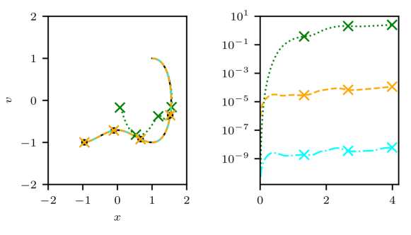
Figure 3: Comparison of the surrogate models with coordinate projection using $\mathbb{V}_{3}$ (4.2; $--$), coordinate projection using $\mathbb{V}_{5}$ (4.2; $\cdot-$) and no projection using $\mathbb{V}_{5}$ (4.5; $\cdots$) for Example 4 on $\mathbb{X}=[-2,2]^{2}$ in comparison to the exact solution (—): exemplary trajectories (left) and mean error over time averaged over $x^{0}\in\mathbb{X}$ (right).

While the additional projection step typically yields a significant improvement of the approximation quality, we provide some additional insight why the coordinate projection is particularly well suited for the Duffing oscillator considered in Example 4. The reasoning is the close relationship between the system equations (4.3) and the choice of the dictionary $\mathbb{V}_{5}$, which can be shown in a more general fashion: Let $\mathbb{V}$ be a dictionary including the coordinate functions, i.e., $\Psi$ can be written as (2.3), and assume that $f_{i}\in\mathbb{V}$ holds for $i\in[1:d]$ (each component of the right hand side (2.1) is contained in the dictionary). The representation (2.3) allows to rewrite the argument of the regression problem (2.4) as

$$\|\Psi(x(t;\hat{x}))-K\Psi(\hat{x})\|^{2}_{2}\!=\!\left\|\begin{pmatrix}x(t;\hat{x})-K_{[1:d]}\Psi(\hat{x})\\ \bar{\Psi}(x(t;\hat{x}))-K_{[d+1:N]}\Psi(\hat{x})\end{pmatrix}\right\|^{2}_{2}\!\!=\!\left\|\begin{pmatrix}\hat{x}+tf(\hat{x})+\mathcal{O}(t^{2})-K_{[1:d]}\Psi(\hat{x})\\ \bar{\Psi}(x(t;\hat{x}))-K_{[d+1:N]}\Psi(\hat{x})\end{pmatrix}\right\|^{2}_{2}\!\!,$$

where we tacitly imposed sufficient smoothness of the vector field $f$ such that $x(t;\hat{x})=\hat{x}+tf(\hat{x})+\mathcal{O}(t^{2})$ holds. Then, invoking $f_{i}\in\mathbb{V}$, the approximation error of the solution $\hat{K}_{[1:d]}$ is bounded by $\mathcal{O}(t^{2})$. In particular, we obtain

$$\hat{F}_{\pi}(\hat{x})=x(t;\hat{x})+\mathcal{O}(t^{2})$$

for all initial conditions $\hat{x}\in\mathbb{X}$.

5 Closest-Point Projections

In the following we assume that the set $M$ defined by (3.1), which is induced by $\Psi\in L^{2}(\mathbb{X},\mathbb{R})^{N}$, is a smooth and $d$-dimensional embedded manifold in $\mathbb{R}^{N}$, where continuous differentiability is a sufficient smoothness assumption for our purposes. Alternatively, one may consider any injective immersion $\Psi$ which satisfies any of the conditions of [12, Proposition 4.22].

Let $W\in\mathbb{R}^{N\times N}$ be a positive semi-definite matrix and define the weighted semi-inner product

$$\langle u_{1},u_{2}\rangle_{W}:=u_{1}^{\top}Wu_{2}\qquad\forall\,u_{1},u_{2}\in\mathbb{R}^{N}.$$

If $W$ is invertible or the weaker condition

$$\det(\mathrm{D}\Psi(x)^{\top}W\mathrm{D}\Psi(x))\neq 0\qquad\forall\,x\in\mathbb{X}$$ (5.1)

holds, then $W$ induces a Riemannian metric on $M$. This then defines the notion of distance on the manifold $M$.

Based on the chosen semi-inner product $\langle\cdot,\cdot\rangle_{W}$, we construct the closest-point projection.

Definition 5.

For a given $(N\times N)$-matrix $W=W^{\top}\geq 0$ satisfying Condition (5.1), the closest-point projection $\pi_{W}:\mathbb{R}^{N}\to M$ is defined as

$$\pi_{W}(z):=\operatorname{argmin}_{p\in M}\|z-p\|_{W}.$$ (5.2)

Condition (5.1) ensures that $\pi_{W}$ is well-defined in a neighbourhood of the manifold embedded in $\mathbb{R}^{N}$, and, in particular, $\pi_{W}(z)=z$ for all $z\in{M}$. Since the projection operator (5.2) is invariant under scalings of $W$, i.e., $\pi_{W}(z)=\pi_{\alpha W}(z)$ holds for all $z\in\mathbb{R}^{N}$ and $\alpha>0$, it suffices to consider semi-inner product $W$ satisfying ${\det}^{\dagger}(W)=1$. This corresponds to the choices of $W$ for which the Riemannian volume of $M$ is constant.

Next, we show that the coordinate projection is a closest-point projection.

Proposition 6.

Let $\Psi$ be given by Equation (2.3), i.e., $\Psi$ contains the coordinate functions. Then,

$$C:=\begin{pmatrix}I_{d}&0_{d\times N-d}\\ 0_{N-d\times d}&0_{N-d\times N-d}\end{pmatrix}\in\mathbb{R}^{N\times N}$$ (5.3)

induces a Riemannian metric on ${M}$, and the coordinate projection (4.1) coincides with the closest-point projection with $W=C$.

Proof.

We verify Condition (5.1) to show that $C$ induces a Riemannian metric on ${M}$. Let $x\in\mathbb{X}$ be given. Then, we have $\det(\mathrm{D}\Psi(x)^{\top}C\mathrm{D}\Psi(x))=\det(I_{d})\neq 0$, which can be directly inferred by rewriting the left hand side as

$$\det\left(\begin{pmatrix}I_{d}\\ \mathrm{D}\bar{\Psi}(x)\end{pmatrix}^{\top}\begin{pmatrix}I_{d}&0_{d\times N-d}\\ 0_{N-d\times d}&0_{N-d\times N-d}\end{pmatrix}\begin{pmatrix}I_{d}\\ \mathrm{D}\bar{\Psi}(x)\end{pmatrix}\right).$$

Now, for any $z\in\mathbb{R}^{N}$, one has

$$\pi_{C}(z) =\operatorname{argmin}_{p\in M}\|z-p\|_{C}$$

$$=\Psi\circ\operatorname{argmin}_{x\in\mathbb{X}}\|z-\Psi(x)\|_{C}$$

$$=\Psi\circ\operatorname{argmin}_{x\in\mathbb{X}}\left\|\begin{pmatrix}z_{[1:d]}-x\\ z_{[d+1:N]}-\bar{\Psi}(x)\end{pmatrix}\right\|_{C}$$

$$=\Psi\circ\operatorname{argmin}_{x\in\mathbb{X}}\left\|z_{[1:d]}-x\right\|=\Psi(z_{[1:d]}),$$

which completes the proof. ∎

We emphasize that the matrix $C$ is not invertible. Further, the closest-point projection $\pi_{W}$ is, in general, a nonlinear projection, and, may be implemented using variants of steepest descent or Newton’s method [1].

The following proposition shows that the error resulting from the closest-point projection is proportionally bounded to the approximation error in the regression problem (2.4).

Proposition 7.

The closest point projection of Definition 5 satisfies

$$\left\|\pi_{W}(\hat{K}\Psi(x))-\mathcal{K}^{t}\Psi(x)\right\|_{W}\leq 2\left\|\hat{K}\Psi(x)-\mathcal{K}^{t}\Psi(x)\right\|_{W}$$

for all $x\in\mathbb{R}^{d}$. That is, its error is bounded by twice the training error in the given metric $W$.

Proof.

Since $\mathcal{K}^{t}\Psi(x)\in M$, the definition of $\pi_{W}(\hat{K}\Psi(x))$ implies

$$\left\|\pi_{W}(\hat{K}\Psi(x))-\hat{K}\Psi(x)\right\|_{W}\leq\left\|\mathcal{K}^{t}\Psi(x)-\hat{K}\Psi(x)\right\|_{W}.$$

Hence, using the triangle inequality and the definition of the regression problem (2.4) weighted with $W$ yields the assertion. ∎

One may observe that the bound of Proposition 7 uses the semi-inner product $W$, which is not the metric used in the construction of the surrogate model $\hat{K}$, cp. the regression problem (2.4). However, we show in the following proposition that the solution of problem (2.4) also solves the weighted regression problem.

Proposition 8.

The solution $\hat{K}$ to the regression problem (2.4) satisfies

$$\hat{K} \in\operatorname{arg}\min_{K\in\mathbb{R}^{N\times N}\hskip 11.38092pt}\int_{\mathbb{X}}\|\Psi(x(t;\hat{x}))-K\Psi(\hat{x})\|^{2}_{W}\,\mathrm{d}\hat{x}$$ (5.4)

for all $W=W^{\top}\geq 0$, $W\in\mathbb{R}^{N\times N}$.

Proof.

Using $\Psi_{X},\Psi_{Y}$ given by (2.5), differentiation of the cost w.r.t. ${K}$ in an arbitrary direction $\Delta$ yields

$$2\int_{\mathbb{X}}\langle K\Psi(\hat{x})-\Psi(x(t;\hat{x}))\,,\,\Delta\Psi(\hat{x})\rangle_{W}\,\mathrm{d}\hat{x}= 2\langle\int_{\mathbb{X}}K\Psi(\hat{x})\Psi(\hat{x})^{\top}-\Psi(x(t;\hat{x}))\Psi(\hat{x})^{\top}\,\mathrm{d}\hat{x},\Delta\rangle_{W}$$

$$= 2\langle K\Psi_{X}-\Psi_{Y},\Delta\rangle_{W}=2\langle W(K\Psi_{X}-\Psi_{Y}),\Delta\rangle.$$

This expression is nullified for $\hat{K}=\Psi_{Y}\Psi_{X}^{-1}$, which is thus indeed a solution to the regression problem (5.4); independently of the chosen weighting matrix $W=W^{\top}\geq 0$. ∎

6 Geometric Projection

The choice of a suitable metric is a non-trivial task. We propose a geometrically-motivated one, which exhibits a superior performance as demonstrated in this section.

Definition 9.

Let $\Sigma\in\mathbb{R}^{N\times N}$ be given by

$$\Sigma=\int_{\mathbb{X}}(\hat{K}\Psi(x)-\mathcal{K}^{t}\Psi(x))(\hat{K}\Psi(x)-\mathcal{K}^{t}\Psi(x))^{\top}\,\mathrm{d}x$$ (6.1)

and be invertible. Then, the geometric projection $\pi_{W}$ is the closest point projection of Definition 5 associated with the metric $W=\det(\Sigma)^{1/N}\Sigma^{-1}$.

Recalling the scaling invariance, it is straightforward to see that the geometric projection is a special case of closest-point projection with the metric $W=\Sigma^{-1}$, where $\Sigma$ is defined as in (6.1). The geometric projection can be interpreted from a probabilistic viewpoint. Suppose that we approximate the Koopman operator based on normally distributed i.i.d. random variables, i.e., $\hat{K}\Psi(x)\sim N(\mathcal{K}^{t}\Psi(x),\Sigma)$ for every $x\in D$ with $\Sigma$ defined by (6.1). Then, for every $x\in D$, the likelihood of a point $p\in\mathbb{R}^{N}$ being equal to $\mathcal{K}^{t}\Psi(x)$ can be written as

$$\rho(\,p\,|\,\hat{K}\Psi(x))=\frac{\exp\left(-0.5\cdot\|p-\hat{K}\Psi(x)\|_{\Sigma^{-1}}^{2}\right)}{\sqrt{(2\pi)^{N}\det(\Sigma)}}.$$

If we restrict ourselves to look for points $p\in M$, then the maximum likelihood solution is exactly

$$\operatorname{argmax}_{p\in M}\rho(\,p|\,\hat{K}\Psi(x))=\pi_{W}(\hat{K}\Psi(x)),$$

where $W=\Sigma^{-1}$ holds.

Next, we consider the example of a pendulum to demonstrate the advantages of the geometric projection in comparison to its coordinate-based counterpart. To this end, we use the notation $\Delta t$ in the following to indicate the time step, i.e., $\hat{K}$ approximates $\mathcal{K}^{\Delta t}$.

Example 10.

Consider the pendulum with dynamics

$$\dot{x}=v,\qquad\dot{v}=-\sin(x)$$ (6.2)

on the domain $\mathbb{X}=[-\pi,\pi]\times[-3,3]$. We approximate the Koopman operator by taking $10,000$ data points $\hat{x}$ drawn uniformly i.i.d. from $\mathbb{X}$ and the respective solution $x(\Delta t;\hat{x})$ as described in Section 2 using monomial dictionaries $\mathbb{V}_{n}$, $n\in\mathbb{N}$, cp. (4.4).

The projection methods are compared by examining the approximated system dynamics (4.2) with those obtained through a high-order numerical integration scheme with step-size control. The one-step error at a given value $\hat{x}\in\mathbb{X}$ is

$$E_{1-\text{Step}}^{W}(\hat{x}):=\|\hat{F}_{\pi_{W}}(\hat{x})-x(\Delta t;\hat{x})\|$$ (6.3)

for a given projection $\pi_{W}$. Figure 4 shows the one-step errors for the coordinate and geometric projections using the dictionary $\mathbb{V}_{2}$.

Figure 4: Example 10 with dictionary $\mathbb{V}_{2}$: Comparison of the one-step errors (6.3) for the approximated dynamics using coordinate (left) and geometric projection (right), respectively.

For a better comparison and the impact of using, in addition, monomials of order three in the dictionary, Figure 5 shows the difference in one-step errors.

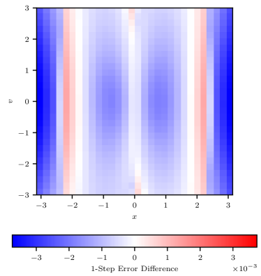
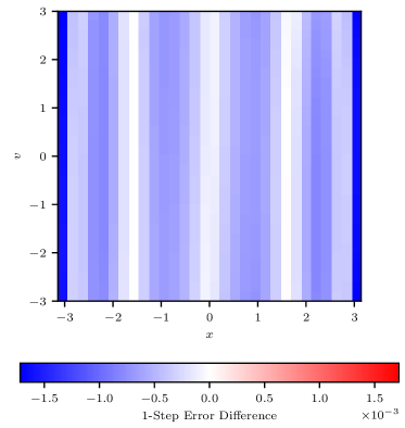
Figure 5: The difference in 1-Step errors $E_{1-\text{Step}}^{W}(\hat{x})-E_{1-\text{Step}}^{C}(\hat{x})$ for the approximated dynamics using geometric and coordinate projections and dictionary orders 2 (left) and 3 (right).

For $\mathbb{V}_{2}$, the geometric projection has a lower one-step error in most of the domain, which is consistent with the underlying regression problem, in which the $L^{2}$-error is minimized. For $\mathbb{V}_{3}$, the geometric projection has a lower one-step error everywhere. The underlying reasoning is that the geometric projection exploits its additional freedom by taking more dictionary elements into account to return to the manifold $M$.

The 1-step error depends on $\Delta t$ for any projection method. Figure 6 shows how the 1-step error statistics change for the coordinate and geometric projections depending on the time step $\Delta t$. Again, the geometric projection clearly outperforms its coordinate-based counterpart if the dictionary size increases, i.e., for $\mathbb{V}_{n}$ and $n\in\{3,4,5\}$ (see Figure 6 for $n=2,3$). Regardless of dictionary size, both projections degrade as the time-step is increased.

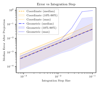
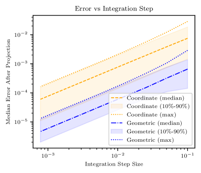
Figure 6: Comparison of median 1-step error for the geometric and coordinate projections using $\mathbb{V}_{2}$ (left) and $\mathbb{V}_{3}$ (right) depending on time step $\Delta t$.

Next, we consider the Lorenz system for a dictionary $\Psi$ without $\psi_{1}(x,y,z)=x$, i.e., the dictionary does not contain all coordinate functions, see also [13, Section III.C].

Example 11.

Consider the Lorenz system given by

$$\dot{x} =\sigma(y-x), \dot{y} =x(\rho-z)-y, \dot{z} =xy-\beta z,$$

on the domain $\mathbb{X}=[-20,20]\times[-20,20]\times[10,50]$.

In this case, the coordinate projection can be realised by selecting three observables from which $x,y,z$ can be recovered: $xz$, $y$, and $z$, i.e., $x$ can be reconstructed by $x=xz/z$ since $z\in[10,50]$. Figure 7 shows an examplary trajectory from the true and approximated dynamics using the dictionary $\mathbb{V}_{4}\setminus\{x\}$. While the geometric projection performs well without the coordinate function, the accuracy of the reconstructed coordinate projection is poor.

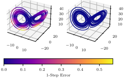
Figure 7: 1-step errors along a sample trajectory of Example 11 for the coordinate (left) and geometric projections (right) using the dictionary $\mathbb{V}_{4}\setminus\{x\}$.

7 Conclusions and outlook

Our key contributions are the following: First, we have demonstrated the need for a reprojection step whenever the dictionary is not Koopman invariant. Second, we proposed a general framework to conduct the reprojection step based on a large class of semi-inner products. In particular, it is not necessary that the coordinate functions are contained in the dictionary to conduct the reprojection step, see, e.g., the novel closest-point projection supposing invertibility of the map $\Psi$. Third, we have rigorously shown that the additional reprojection step essentially maintains the estimation error resulting from the regression problem and, indeed, significantly reduces the approximation error as shown in our numerical simulations. A key reason is that the chosen weighting does not interfere with the regression problem to be solved for computing the data-based compression $\hat{K}$.

Clearly, the proposed framework is directly applicable to nonlinear control-affine systems, if bilinear surrogate models are used, see, e.g., [18, 21] and the references therein. Here, already the coordinate projection has turned out to be very beneficial in simulation and experiments for non-holonomic robots [4] such that we expect clear benefits if the novel geometric projection is applied. This claim also applies to eDMD with control [20] since the weighting $W$ of the control in the augmented state may be set to zero.

Future work might be devoted to leveraging recently introduced concepts [16] for the analysis of systems with a globally-stable attractor in our setting more tailored towards control systems typically lacking such structures. Here, taking into account the recent results of [8] is of interest. Furthermore, we will leverage known results from regression [3] to further analyze and potentially improve the proposed framework.

References

- [1] P.-A. Absil, R. Mahony, and R. Sepulchre. Optimization algorithms on matrix manifolds. In Optimization Algorithms on Matrix Manifolds. Princeton University Press, 2009.
- [2] P. Bevanda, S. Sosnowski, and S. Hirche. Koopman operator dynamical models: Learning, analysis and control. Annu Rev Control, 52:197–212, 2021.
- [3] C. M. Bishop and N. M. Nasrabadi. Pattern recognition and machine learning, volume 4. Springer, 2006.
- [4] L. Bold, H. Eschmann, M. Rosenfelder, H. Ebel, and K. Worthmann. On Koopman-based surrogate models for non-holonomic robots. Preprint arxiv:2303.09144, 2023.
- [5] L. Bold, L. Grüne, M. Schaller, and K. Worthmann. Practical asymptotic stability of data-driven model predictive control using extended DMD, 2023. Preprint available on arXiv.
- [6] S. L. Brunton, B. W. Brunton, J. L. Proctor, and J. N. Kutz. Koopman invariant subspaces and finite linear representations of nonlinear dynamical systems for control. PloS one, 11(2):e0150171, 2016.
- [7] S. L. Brunton, J. L. Proctor, and J. N. Kutz. Discovering governing equations from data by sparse identification of nonlinear dynamical systems. Proceedings of the national academy of sciences, 113(15):3932–3937, 2016.
- [8] D. Goswami and D. A. Paley. Bilinearization, reachability, and optimal control of control-affine nonlinear systems: A Koopman spectral approach. IEEE Transactions on Automatic Control, 67(6):2715–2728, 2021.
- [9] S. Klus, F. Nüske, S. Peitz, J.-H. Niemann, C. Clementi, and C. Schütte. Data-driven approximation of the Koopman generator: Model reduction, system identification, and control. Physica D: Nonlinear Phenomena, 406:132416, 2020.
- [10] M. Korda and I. Mezić. Linear predictors for nonlinear dynamical systems: Koopman operator meets model predictive control. Automatica, 93:149–160, 2018.
- [11] M. Korda and I. Mezić. On convergence of extended dynamic mode decomposition to the Koopman operator. J. Nonlinear Sci., 28(2):687–710, 2018.
- [12] J. M. Lee. Introduction to Smooth manifolds. Springer, 2012.
- [13] Q. Li, F. Dietrich, E. M. Bollt, and I. G. Kevrekidis. Extended dynamic mode decomposition with dictionary learning: A data-driven adaptive spectral decomposition of the Koopman operator. Chaos: An Interdisciplinary J. Nonlinear Sci., 27(10):103111, 2017.
- [14] A. Mauroy and J. Goncalves. Linear identification of nonlinear systems: A lifting technique based on the Koopman operator. In 55th IEEE Conference on Decision and Control (CDC), pages 6500–6505, 2016.
- [15] A. Mauroy, I. Mezić, and Y. Susuki. The Koopman operator in systems and control. Springer Nature, Cham, Switzerland, Feb. 2020.
- [16] I. Mezić. Spectrum of the Koopman operator, spectral expansions in functional spaces, and state-space geometry. Journal of Nonlinear Science, 30(5):2091–2145, 2020.
- [17] F. Nüske, S. Peitz, F. Philipp, M. Schaller, and K. Worthmann. Finite-data error bounds for Koopman-based prediction and control. J. Nonlinear Sci., 33:14, 2023.
- [18] S. E. Otto and C. W. Rowley. Koopman operators for estimation and control of dynamical systems. Annu. Rev. Control Robot. Auton. Syst., 4:59–87, 2021.
- [19] F. Philipp, M. Schaller, K. Worthmann, S. Peitz, and F. Nüske. Error bounds for kernel-based approximations of the Koopman operator, 2023. Submitted, Preprint: arXiv:2301.08637.
- [20] J. L. Proctor, S. L. Brunton, and J. N. Kutz. Generalizing Koopman theory to allow for inputs and control. SIAM J. Appl. Dyn. Syst., 17(1):909–930, 2018.
- [21] M. Schaller, K. Worthmann, F. Philipp, S. Peitz, and F. Nüske. Towards reliable data-based optimal and predictive control using extended DMD. IFAC-PapersOnLine, 56(1):169–174, 2023.
- [22] H. Terao, S. Shirasaka, and H. Suzuki. Extended dynamic mode decomposition with dictionary learning using neural ordinary differential equations. Nonlinear theory appl. IEICE, 12(4):626–638, 2021.
- [23] M. O. Williams, M. S. Hemati, S. T. Dawson, I. G. Kevrekidis, and C. W. Rowley. Extending data-driven Koopman analysis to actuated systems. IFAC-PapersOnLine, 49(18):704–709, 2016.
- [24] M. O. Williams, I. G. Kevrekidis, and C. W. Rowley. A data–driven approximation of the Koopman operator: Extending dynamic mode decomposition. J. Nonlinear Sci., 25:1307–1346, 2015.
- [25] C. Zhang and E. Zuazua. A quantitative analysis of Koopman operator methods for system identification and predictions. Comptes Rendus. Mécanique, 351(S1):1–31, 2023.