Semiclassical descriptions of dissipative dynamics of strongly interacting Bose gases in optical lattices

Abstract

We develop semiclassical methods for describing real-time dynamics of dissipative Bose-Hubbard systems in a strongly interacting regime, which can be realized in experiments with ultracold gases. Specifically, we present two kinds of SU(3) truncated Wigner approximation (TWA) for solving an effective Lindblad master equation of the systems. The first one employs the discrete TWA for finite levels or spin systems and is based on a classical equation of motion in which the onsite dissipation term, as well as the onsite interaction term, is linearized in the phase space variables. The other approach utilizes a stochastic Langevin equation, including decoherence effects in terms of nonlinear drift force and stochastic force terms, in which the initial conditions of trajectories are weighted with a quasiprobability distribution for a typical initial quantum state. We apply these methods to the systems with two-body losses and compare their results with the exact numerical solutions for a small system. We show that the former approach can simulate correctly longer-time dynamics than the latter one. We also calculate the time evolution for a large size setup that is comparable to experiments. We numerically demonstrate that the discrete TWA approach is able to qualitatively capture the continuous quantum Zeno effect on dynamics subjected to a gradual change of the ratio between the hopping amplitude and the onsite interaction across the superfluid-Mott insulator crossover, which has been observed experimentally.

I Introduction

Rapid growth of technology for manipulating ultracold gases has enabled one to implement analog quantum simulators of open quantum many-body systems Müller et al. (2012); Schäfer et al. (2020); Altman et al. (2021); Diehl et al. (2008). Recent experiments have indeed realized interacting lattice systems with controllable dissipation, such as one-body losses Barontini et al. (2013); Labouvie et al. (2016), two-body losses Tomita et al. (2017); Honda et al. (2022), and inelastic photon scattering Patil et al. (2015); Lüschen et al. (2017); Bouganne et al. (2020). These artificial systems have been utilized as platforms for exploring novel macroscopic states and dynamics of many-body systems beyond the paradigm of equilibrium and nonequilibrium physics of isolated systems. Recent experimental studies on Bose gases in optical lattices include the observations of bistability in steady states caused by one-body losses Labouvie et al. (2016), anomalous subdiffusion of superfluid coherence in the presence of both two-body losses and inelastic photon scattering Bouganne et al. (2020), and the delay in melting of the Mott insulator due to the continuous quantum Zeno effects resulting from two-body losses Tomita et al. (2017). Such exploration of the nontrivial interplays between dissipation and many-particle correlations is relevant also to understanding and controlling various other systems, e.g., Bose-Einstein condensates coupled to optical cavity modes Brennecke et al. (2013); Chiacchio and Nunnenkamp (2019); Keßler et al. (2021), trapped ions Barreiro et al. (2011); Lin et al. (2013), and superconducting qubits inside a cavity Leghtas et al. (2013); Chen et al. (2022).

For further improvement of quantum simulators for open many-body systems, it is important to develop a numerical tool that can evaluate nontrivial outputs associated with the combined effects of interparticle interactions and dissipation. However, reliable and efficient classical simulations of real time evolution of a dissipative many-body system is in general hard mainly due to the exponential growth of the Hilbert-space dimension with respect to the system size. While some computational methods based on tensor networks have been developed and utilized Schröder et al. (2019); Luchnikov et al. (2019); Goto and Danshita (2020); Nakano et al. (2021), their efficient applications are typically limited to low entangled states in one dimension as in the case of isolated systems.

For higher dimensional open systems, there are various time-dependent mean-field approaches that can approximately evaluate the time dependence of local observables governed by microscopic master equations for mixed states. For instance, in Ref. Tomita et al. (2017), the time-dependent Gutzwiller approximation method Diehl et al. (2010); Tomadin et al. (2011) is employed to analyze the time evolution of a dissipative Bose-Hubbard system with two-body losses. It has been numerically shown that a site decoupling ansatz for many-body mixed states can nicely recover some qualitative features of the Zeno effect that can be observed in the local atomic density Tomita et al. (2017). However, in the Gutzwiller approach, for inducing crossover from a Mott insulator phase to a superfluid phase, one needs to introduce artificial noises as small perturbations. Such noises inevitably cause uncontrolled errors, leading to quantitative inaccuracy in the results. Moreover, due to its site decoupling nature, the Gutzwiller approach cannot properly describe offsite correlation functions. This drawback significantly limits the application of the Gutzwiller approach to ultracold-gas systems, e.g., not being able to evaluate the momentum distribution of atomic gases, an indispensable observable measured via time-of-flight images, because it is usually computed as a sum of offsite single-particle correlation functions in real space.

We also note that a dynamical mean-field theory (DMFT) approach based on a single-site impurity solver has been proposed to describe the quantum Zeno effect in higher dimensional dissipative Bose-Hubbard systems Seclì et al. (2022). Even though the DMFT approach is expected to be more quantitative than the Gutzwiller approach, it is not straightforward to calculate spatial correlation functions either. This difficulty stems from the locality of the formulation, in which the system sites are decomposed into an impurity site and its surrounding mean-field bath with only frequency dependence.

In this paper, we present truncated Wigner phase space methods for semiclassically analyzing dissipative dynamics of strongly interacting Bose-Hubbard systems. Phase space methods based on quasiprobability distributions such as the Wigner function, Husimi function, and Glauber-Sudarshan $P$ function provide a versatile tool to analyze open quantum systems Gardiner and Zoller (2004). In particular, the truncated Wigner approximation (TWA) in the Wigner function representation has recently emerged as a powerful semiclassical framework for approximately solving real time evolution of dissipative quantum systems coupled to the environment Keßler et al. (2020); Seibold et al. (2020); Hao et al. (2021); Huber et al. (2021); Singh and Weimer (2022); Mink et al. (2022); Huber et al. (2022). A generic feature of the TWA is that the dynamics of a quantum system is replaced with a set of fluctuating classical trajectories on phase space, whose initial conditions are statistically weighted with an initial state Wigner function expressing quantum fluctuations.

In a typical way of semiclassically expressing the dynamics of the isolated Bose-Hubbard model in its weakly interacting regime, trajectories are generated by the Hamilton equation for complex-valued field amplitudes, i.e., the discrete Gross-Pitaevskii (GP) equation Blakie et al. (2008); Polkovnikov (2010); Nagao et al. (2019); Ozaki et al. (2020). Although the TWA based on the GP equation no longer provides an appropriate description in the strongly interacting regime, there is an alternative representation, namely, the SU(3) TWA, which exactly describes onsite particle and hole fluctuations in strongly interacting states Davidson and Polkovnikov (2015); Fujimoto et al. (2020); Nagao et al. (2021). In this method, the equation of motion in the classical limit is given as the Hamilton equation for SU(3) pseudospin variables, and it is formally equivalent to the time dependent variational equation in the single-site Gutzwiller mean-field theory Nagao et al. (2021). However, in the case of a driven dissipative system, which is not governed by the von-Neumann equation for isolated systems, the classical trajectories cannot be accurately reproduced via the Hamilton equations alone. This is because dissipative forces emerge in addition to the Hamiltonian dynamics, representing the effects of decoherence that influence the coherent time evolution.

As a key step to the goal of realizing an efficient large scale classical simulation of the experimental setup, here in this paper, we develop and use two types of the generalized SU(3) TWA method to analyze an effective Lindblad master equation for the dissipative analog quantum simulator. The first approach is a discrete TWA (dTWA) formulation Schachenmayer et al. (2015); Kunimi et al. (2021) for the master equation and gives a direct generalization of the SU(3) dTWA representation for the isolated Bose-Hubbard model, which was previously discussed in Ref. Nagao et al. (2021). The second one is based on a continuous TWA representation of the Markovian time evolution built with a stochastic Langevin equation and a continuous Wigner distribution for the initial state. Since the Langevin equation derived here for the SU(3) TWA is inevitably nonlinear with respect to the dissipation strength in the master equation, such a description is merely approximate for any dissipation strength even if the offsite term, i.e., the hopping term in the Hamiltonian, is absent. By contrast, the classical equation of motion appearing in the dTWA formalism is linear with respect to the onsite dissipation strength, thus implying that the onsite two-body losses can be exactly captured independently of the dissipation strength. Therefore, an improved accuracy of the semiclassical description is anticipated in the first approach.

We demonstrate that these two different TWA approaches can qualitatively describe the continuous quantum Zeno effect in the non-unitary dynamics with strong dissipation. However, the resulting threshold of the dissipation strength for exhibiting the Zeno effect is different, depending on which approach is employed for the simulation. In particular, we show that, because of the linearity of the non-unitary contributions in the classical limit, the dTWA representation can produce reasonable threshold values of the dissipation strength separating Zeno and non-Zeno regimes in comparison with the experimental results on the time evolution of the atomic density as well as the momentum distribution.

The rest of this paper is organized as follows. In Sec. II, we introduce an effective Lindblad master equation for onsite two-body losses of the atoms in the quantum simulator. In Sec. III, we describe two different SU(3) TWA formalisms for the master equation, which are not equivalent to each other in the presence of dissipation. In Sec. IV, we show the numerical results to investigate the continuous Zeno effect. In Sec. V, we conclude this paper and describe future perspectives.

II Model

The system considered in this paper is an open quantum many-body system with controllable dissipation of local inelastic two-body losses. The relevant experimental system is a cold atomic analog quantum simulator reported in Ref. Tomita et al. (2017), where a highly-controlled dissipative Bose-Hubbard system is successfully realized, as outlined below.

In Ref. Tomita et al. (2017), Tomita et al. utilized a single-photon photoassociation (PA) laser technique to realize a controllable dissipative system built with ${}^{174}{\rm Yb}$ bosonic atoms in a three dimensional optical lattice. Shining a PA laser beam to this optical lattice system may convert pairs of two atoms doubly occupying the same site into ${}^{1}S_{0}+{}^{3}P_{1}$ molecules Tomita et al. (2017). These molecules are immediately disassociated into the two ground-state atoms with high kinetic energy, and thus these disassociated atoms escape from the system, as schematically illustrated in Fig. 1. An important point of this setup is that the strength of such an onsite inelastic two-body collision loss can be readily controlled via tuning the intensity of PA laser.

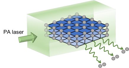
Figure 1: Schematic illustration of the analog quantum simulation experiment for a driven dissipative Bose-Hubbard system in Ref. Tomita et al. (2017). In order to effectively induce two-body loss dissipation, a PA laser is shined to an atomic system comprised of ${}^{174}{\rm Yb}$ atoms in a three-dimensional optical lattice.

The atomic system that is coherently coupled to the photo-associated molecular state is described by the Markovian-Lindblad master equation with a one-body loss Kraus operator for the molecules Tomita et al. (2017); Rousseau and Denteneer (2008). However, our focus is on the real-time dynamics of the atomic sector of this atom-molecule coupled system. We therefore define an effective density matrix operator ${\hat{\rho}}_{\rm eff}$ only for the atoms by adiabatically erasing the molecular degrees of freedom from the total density matrix of the composite system Tomita et al. (2017). This step can be carried out by using second order perturbation theory with some projection operators for the master equation. The time evolution equation for ${\hat{\rho}}_{\rm eff}$ is then found to be an effective Lindblad master equation that only includes the atomic field operators, i.e.,

$$\hbar\frac{\partial}{\partial t}{\hat{\rho}}_{\rm eff}=-i[{\hat{H}}_{\rm BH},{\hat{\rho}}_{\rm eff}]+L_{2}[{\hat{\rho}}_{\rm eff}].$$ (1)

The first commutator term expresses the unitary contribution to the dynamics generated by the Bose-Hubbard Hamiltonian in three dimensions Jaksch et al. (1998)

$${\hat{H}}_{\rm BH}=-J\sum_{\langle j,k\rangle}({\hat{a}}^{\dagger}_{j}{\hat{a}}_{k}+{\rm H.c.})+\frac{U}{2}\sum_{j}{\hat{a}}^{\dagger}_{j}{\hat{a}}^{\dagger}_{j}{\hat{a}}_{j}{\hat{a}}_{j},$$ (2)

where ${\hat{a}}_{j}$ and ${\hat{a}}^{\dagger}_{j}$ are the bosonic annihilation and creation operators at site $j$, respectively, satisfying the commutation relations $[{\hat{a}}_{j},{\hat{a}}^{\dagger}_{l}]=\delta_{j,l}$. $J$ and $U$ represent the hopping amplitude and the onsite interaction strength, respectively, and they are defined as functions of the optical lattice depth that can be readily controlled in the experimental setup.

In Eq. (1), the dissipative contribution in the presence of the PA laser is described by the non-unitary term $L_{2}[{\hat{\rho}}_{\rm eff}]$. For the setup that we consider here, the onsite losses of atoms are represented by

$$L_{2}[{\hat{\rho}}_{\rm eff}]=\frac{\hbar\Gamma_{\rm PA}}{4}\sum_{j}\left[2{\hat{a}}_{j}{\hat{a}}_{j}{\hat{\rho}}_{\rm eff}{\hat{a}}^{\dagger}_{j}{\hat{a}}^{\dagger}_{j}-\{{\hat{a}}^{\dagger}_{j}{\hat{a}}^{\dagger}_{j}{\hat{a}}_{j}{\hat{a}}_{j},{\hat{\rho}}_{\rm eff}\}\right],$$

where $\{\cdot,\cdot\}$ is the anti-commutator bracket. The inelastic collision rate $\Gamma_{\rm PA}$ is expressed as $\Gamma_{\rm PA}=\beta_{\rm PA}\int d{\bf r}|w({\bf r})|^{4}$, where $w({\bf r})$ is the lowest band Wannier function as a function of the lattice depth and $\bf r$ is the coordinate vector in real space. The coefficient $\beta_{\rm PA}$ can be controlled by varying the intensity of the PA laser, as described above. For more details, see also Ref. Tomita et al. (2017).

The controllability of the collision rate $\Gamma_{\rm PA}$ has been utilized in Ref. Tomita et al. (2017) to explore the continuous quantum Zeno effect on coherent many-body dynamics in the strongly interacting regime of the three-dimensional lattice system. This effect occurs as suppression of coherent tunneling processes between neighboring sites caused by strong dissipation of losses Zhu et al. (2014); Patil et al. (2015); Tomita et al. (2017); Asai et al. (2022); Honda et al. (2022). The quantum Zeno effect in many-body systems has also been an important concept in recent studies associated with measurement-induced entanglement transitions on quantum circuits Li et al. (2019); Koh et al. (2022). In the following, we analyze driven-dissipative dynamics of the experimental system by using SU(3) TWA methods for the master equation in Eq. (1). As a key consequence demonstrating the effectiveness of the SU(3) TWA, we will show that this approximation can qualitatively capture the dissipation-induced delay of the coherent time evolution, i.e., the continuous Zeno effect, observed experimentally in the atomic density and the momentum distribution of the system Tomita et al. (2017).

III Methods

The effective Lindblad master equation in Eq. (1) is a linear differential equation in the Hilbert space of the bosonic atoms. In the experiment, the onsite interaction $U$ is typically tuned to be in a sufficiently large value as compared with the hopping amplitude $J$, i.e., $U\gg J$. This condition implies that the relevant single-particle states of onsite occupation are only a few states around a mean filling state Altman and Auerbach (2002); Nagao et al. (2018, 2021). In this paper, we assume that the mean filling state at each site is the unit filling state $|1\rangle$, and the relevant onsite excitations around it are the vacuum state $|0\rangle$ and the doubly occupied state $|2\rangle$. Therefore, the Hilbert space dimension to be considered here is $n_{3,N}=3^{N}$, where $N$ represents the total number of sites. In this reduced Hilbert space, any physical operator, including the Bose-Hubbard Hamiltonian and the effective density matrix, can be represented as an expansion in tensor products of three-dimensional SU(3) base matrices such as the Gell-Mann matrices Georgi (2000).

III.1 SU(3) matrix representation of the dissipative Bose-Hubbard system

In order to approximately solve the effective Lindblad master equation in the reduced Hilbert space, we generalize the SU(3) TWA method to the controllable open quantum many-body system. An advantageous property of the SU(3) TWA is that the onsite interaction term in the Hamiltonian is transformed to a linear function of classical SU(3) spin variables, while the offsite hopping term after the transformation still takes the form of a nonlinear function. Therefore, for the strong interaction strength implying $U\gg J$, the classical equation of motion for SU(3) variables is found to have weak nonlinearity. Hence, the semiclassical description of the quantum dynamics is expected to be reasonable over a valid timescale, which can be longer than that for the conventional TWA with the GP equation Nagao et al. (2021). Previously, the SU(3) TWA was applied only for isolated systems Davidson and Polkovnikov (2015); Fujimoto et al. (2020); Nagao et al. (2021).

First, we briefly summarize how one effectively represents the dissipative Bose-Hubbard system in terms of SU(3) pseudospin variables. Let us define SU(3) pseudospin operators ${\hat{X}}^{(j)}_{\alpha}=({\hat{X}}^{(j)}_{\alpha})^{\dagger}$ $(\alpha=1,\cdots,8)$ acting on the reduced Hilbert space with the total dimension $n_{3,N}$. Each of these operators has a finite-dimensional tensor product representation as

$${\hat{X}}^{(j)}_{\alpha}\Leftrightarrow I\otimes\cdots I\otimes\underbrace{T_{\alpha}}_{j\text{\rm th}}\otimes I\otimes\cdots,$$ (3)

where eight Hermitian matrices $T_{\alpha}$ are referred to as SU(3) base matrices and $I$ is the three-dimensional unit matrix. The SU(3) base matrices are assumed to satisfy the $su(3)$ Lie algebras $[T_{\alpha},T_{\beta}]=if_{\alpha\beta\gamma}T_{\gamma}$ with a structure factor tensor $f_{\alpha\beta\gamma}$ and the repeated Greek indices imply Einstein’s convention for summation. With this definition, the SU(3) operators recast the commutation relations $[{\hat{X}}^{(j)}_{\alpha},{\hat{X}}^{(l)}_{\beta}]=if_{\alpha\beta\gamma}{\hat{X}}^{(j)}_{\gamma}\delta_{j,l}$. In this paper, we employ a conventional notation for the explicit matrix form of $T_{\alpha}$, which was also adopted in Refs. Davidson and Polkovnikov (2015); Nagao et al. (2021), i.e.,

$$T_{1} =\frac{1}{\sqrt{2}}\begin{bmatrix}0&1&0\\ 1&0&1\\ 0&1&0\end{bmatrix},\;\;\;T_{2}=\frac{1}{\sqrt{2}}\begin{bmatrix}0&-i&0\\ i&0&-i\\ 0&i&0\end{bmatrix},$$

$$T_{3} =\begin{bmatrix}1&0&0\\ 0&0&0\\ 0&0&-1\end{bmatrix},\;\;\;\;\;\;T_{4}=\begin{bmatrix}0&0&1\\ 0&0&0\\ 1&0&0\end{bmatrix},$$ (4)

$$T_{5} =\begin{bmatrix}0&0&-i\\ 0&0&0\\ i&0&0\end{bmatrix},\;\;\;\;\;\;\;T_{6}=\frac{1}{\sqrt{2}}\begin{bmatrix}0&-1&0\\ -1&0&1\\ 0&1&0\end{bmatrix},$$

$$T_{7} =\frac{1}{\sqrt{2}}\begin{bmatrix}0&i&0\\ -i&0&-i\\ 0&i&0\end{bmatrix},\;\;\;T_{8}=\frac{1}{\sqrt{3}}\begin{bmatrix}-1&0&0\\ 0&2&0\\ 0&0&-1\end{bmatrix}.$$

In the reduced Hilbert space, each annihilation operator reduces to a linear combination of the SU(3) operators, i.e.,

$${\hat{a}}_{j} \rightarrow|0\rangle\langle 1|_{j}+\sqrt{2}|1\rangle\langle 2|_{j}$$

$$\;\;\;=p_{1}{\hat{X}}_{1}^{(j)}+ip_{1}{\hat{X}}_{2}^{(j)}+p_{2}{\hat{X}}_{6}^{(j)}+ip_{2}{\hat{X}}_{7}^{(j)}.$$ (5)

Here, we assume that the highest (lowest) weight of $T_{3}$ corresponds to the local vacuum state $|0\rangle$ (the doubly occupied state $|2\rangle$). The linear coefficients of Eq. (5) are then uniquely determined as $p_{1}=\frac{1+\sqrt{2}}{2\sqrt{2}}$ and $p_{2}=\frac{\sqrt{2}-1}{2\sqrt{2}}$. Moreover, because of the linearization property of $T_{\alpha}$, implying that any polynomial of $T_{\alpha}$ can be recasted into a linear combination of $T_{\alpha}$ and $I$, the quadratic particle density operator ${\hat{n}}_{j}={\hat{a}}^{\dagger}_{j}{\hat{a}}_{j}$ becomes

$${\hat{n}}_{j}\rightarrow 1-{\hat{X}}_{3}^{(j)},$$ (6)

and the onsite interaction operator ${\hat{a}}^{\dagger}_{j}{\hat{a}}^{\dagger}_{j}{\hat{a}}_{j}{\hat{a}}_{j}$ is represented as

$${\hat{a}}^{\dagger}_{j}{\hat{a}}^{\dagger}_{j}{\hat{a}}_{j}{\hat{a}}_{j}\rightarrow\frac{2}{3}-{\hat{X}}^{(j)}_{3}-\frac{1}{\sqrt{3}}{\hat{X}}^{(j)}_{8}.$$ (7)

Combining these results, the Bose-Hubbard Hamiltonian is replaced with a SU(3) spin Hamiltonian. Its explicit form is given in Ref. Nagao et al. (2021). The simplified Hamiltonian is composed of a linear term of the SU(3) pseudospin operators, which is proportional to $U$, and a nonlinear term, which is proportional to $J$. If $J=0$, the unitary time evolution governed by the von-Neumann equation with the Hamiltonian is exactly described in this semiclassical approximation Nagao et al. (2021).

For applications to the effective Lindblad master equation in Eq. (1), the dissipative $L_{2}$ term has also to be rewritten in the pseudospin operators. Because of the linearization property of the base matrices, the two-body loss operator ${\hat{a}}^{2}_{j}$ for the doubly occupied sites, which provides the Kraus measurement operator in constructing $L_{2}[{\hat{\rho}}_{\rm eff}]$, also reads as a linear combination of ${\hat{X}}_{4}^{(j)}$ and ${\hat{X}}_{5}^{(j)}$, i.e.,

$${\hat{a}}^{2}_{j}\rightarrow\frac{1}{\sqrt{2}}{\hat{X}}_{4}^{(j)}+i\frac{1}{\sqrt{2}}{\hat{X}}_{5}^{(j)}.$$ (8)

Note that offsite dissipative terms spreading over multiple sites, which arise, e.g., in a dissipative hard-core boson system in Ref. García-Ripoll et al. (2009), cannot be straightforwardly linearized in onsite phase space variables of spins.

III.2 Method I: dTWA

Let us now explain the dTWA Schachenmayer et al. (2015); Piñeiro Orioli et al. (2017); Kunimi et al. (2021); Singh and Weimer (2022) to approximately calculate the time evolution of the dissipative interacting SU(3) spin system. The dTWA method for finite levels or spin systems formally uses a phase point operator to expand the density matrix operator. For the case of SU(3) spin systems with $N$ sites, an appropriate definition of phase point operator is given via its matrix representation, i.e., ${\mathscr{A}}^{\otimes N}=\bigotimes_{j=1}^{N}{\mathscr{A}}^{[j]}$ with ${\mathscr{A}}^{[j]}=\frac{1}{3}I+\frac{1}{2}{\bm{r}}^{(j)}\cdot{\bm{T}}$ Nagao et al. (2021) and the normalization conditions of $T_{\alpha}$ being ${\rm Tr}(T_{\alpha}T_{\beta})=2\delta_{\alpha\beta}$. Moreover, ${\bm{r}}^{(j)}=(r^{(j)}_{1},\cdots,r^{(j)}_{8})$ represents a spinor vector of eight real-valued discrete parameters. Using the phase point operator, one can expand the initial density matrix at $t=0$ such that $\rho(t=0)=\prod_{j}\sum_{{\bm{r}}^{(j)}}{\mathscr{W}}({\bm{r}}^{(1)},\cdots,{\bm{r}}^{(N)}){\mathscr{A}}^{\otimes N}$. The expansion coefficient ${\mathscr{W}}({\bm{r}}^{(1)},\cdots,{\bm{r}}^{(N)})$ is interpreted as a discrete Wigner function associated with the phase point operator. For a direct product state over real space, the discrete Wigner function is given as a spatially factorized distribution function, i.e., ${\mathscr{W}}({\bm{r}}^{(1)},\cdots,{\bm{r}}^{(N)})=\prod_{j}{\mathscr{W}}_{1}^{[j]}({\bm{r}}^{(j)})$. The local distribution ${\mathscr{W}}_{1}^{[j]}({\bm{r}}^{(j)})$ depends only on ${\bm{r}}^{(j)}$. The explicit form of ${\mathscr{W}}_{1}^{[j]}({\bm{r}}^{(j)})$ that we use in the main calculations will be introduced later.

With the initial density matrix expanded with the phase point operator described above, we now consider the non-unitary time evolution of the phase point operator, which is also generated by the effective Lindblad master equation in Eq. (1). Let us introduce a time-dependent phase point operator at time $t$ as ${\hat{\mathscr{A}}}^{\otimes N}_{t}[\{{\bm{r}}^{(k)}\}_{k=1}^{N}]$ with the initial condition ${\hat{\mathscr{A}}}^{\otimes N}_{t=0}={\hat{\mathscr{A}}}^{\otimes N}$. This operator has to evolve according to

$$\hbar\frac{\partial}{\partial t}{\hat{\mathscr{A}}}^{\otimes N}_{t}=-i[{\hat{H}}_{\rm BH},{\hat{\mathscr{A}}}^{\otimes N}_{t}]+L_{2}[{\hat{\mathscr{A}}}^{\otimes N}_{t}],$$ (9)

where ${\hat{H}}_{\rm BH}$ is expressed in terms of ${\hat{X}}^{(j)}_{\alpha}$. Moreover, we introduce one-site reduced phase point operators ${\mathscr{A}}_{j}^{(1)}(t)={\rm Tr}_{\underline{j}}{\mathscr{A}}^{\otimes N}_{t}$. Here, $\underline{j}$ denotes a trace operation over all sites except for site $j$. In parallel to this, two-site ones, three-site ones, and more higher rank ones are successively defined as ${\mathscr{A}}_{j,j^{\prime}}^{(2)}={\rm Tr}_{{\underline{j}},{\underline{j}}^{\prime}}{\mathscr{A}}^{\otimes N}_{t}$, ${\mathscr{A}}_{j,j^{\prime},j^{\prime\prime}}^{(3)}={\rm Tr}_{{\underline{j}},{\underline{j}}^{\prime},{\underline{j}}^{\prime\prime}}{\mathscr{A}}^{\otimes N}_{t}$, and so on. The time evolution equation of ${\mathscr{A}}_{j}^{(1)}$ is derived by tracing the $N-1$ site indices in Eq. (9). However, it is not a closed equation by ${\mathscr{A}}_{j}^{(1)}$ themselves. Indeed, some inseparable correlations in ${\mathscr{A}}_{j,j^{\prime}}^{(2)}$, i.e., ${\mathscr{B}}_{j,j^{\prime}}^{(2)}\equiv{\mathscr{A}}_{j,j^{\prime}}^{(2)}-{\mathscr{A}}_{j}^{(1)}{\mathscr{A}}_{j^{\prime}}^{(1)}$ may appear in the determination. In order to update the values of ${\mathscr{A}}_{j,j^{\prime}}^{(2)}$, the information of ${\mathscr{A}}_{j,j^{\prime},j^{\prime\prime}}^{(3)}$ is necessary, and more generally, updating ${\mathscr{A}}_{j,j^{\prime},\cdots}^{(s-1)}$ requires ${\mathscr{A}}_{j,j^{\prime},j^{\prime\prime},\cdots}^{(s)}$ at the past step. This hierarchy is known as the Bogoliubov–Born–Green–Kirkwood–Yvon (BBGKY) hierarchy in dynamics of multipoint correlation functions Pucci et al. (2016).

To truncate this hierarchy within the accuracy of dTWA, each two-site operator is approximated to a factorized operator ${\mathscr{A}}^{(2)}_{j,j^{\prime}}={\mathscr{A}}^{(1)}_{j}{\mathscr{A}}^{(1)}_{j^{\prime}}$, i.e., ${\mathscr{B}}_{j,j^{\prime}}^{(2)}=0$. Hence, the time evolution of the one-site operators can be determined in a closed manner. More explicitly, this approximation is equivalent to making a direct product ansatz, namely ${\mathscr{A}}^{\otimes N}_{t}[\{{\bm{r}}^{(k)}\}_{k=1}^{N}]=\bigotimes_{j}{\mathscr{A}}_{j,{\rm dTWA}}^{(1)}$ with ${\mathscr{A}}_{j,{\rm dTWA}}^{(1)}=\frac{1}{3}I+\frac{1}{2}{\bm{r}}^{(j)}_{\rm cl}(t;\{{\bm{r}}^{(k)}\}_{k=1}^{N})\cdot{\bm{T}}$. The time dependent parameters ${\bm{r}}^{(j)}_{\rm cl}(t)$, which are generally nonlinear functions of their initial values ${\bm{r}}^{(j)}={\bm{r}}^{(j)}_{\rm cl}(t=0)$, behave as a set of phase space variables propagated by a classical equation of motion. Quantum fluctuations in the initial state are incorporated in the discrete Wigner function ${\mathscr{W}}$. In numerical simulations, this Wigner function makes a statistical ensemble of ${\bm{r}}^{(j)}_{\rm cl}(t)$ to produce dynamical formation of offsite spatial correlations Kunimi et al. (2021).

Notice that, reflecting the trace conserving property of the time evolution generator in the master equation, which implies that $\langle{\hat{1}}\rangle(t)=1$ holds for all time, the coefficient in front of $I$ remains constant in ${\mathscr{A}}_{j,{\rm dTWA}}^{(1)}$. However, it is not necessarily the case if the non-unitary time evolution belongs to a specific class, such as non-unitary dynamics for a non-Hermitian Hamiltonian, which violates the normalization of the wave functions. A substantial discussion on this issue is found in Ref. Singh and Weimer (2022), where the authors attempt to solve the dTWA equation for the single site operator by adopting the quantum jump method, which requires semiclassical evaluations of quantum trajectories produced by a non-Hermitian Hamiltonian.

Hereinafter, we identify the time evolution equation of ${\bm{r}}^{(j)}_{\rm cl}$. The variables ${\bm{r}}^{(j)}_{\rm cl}$ are nothing but the discrete Weyl symbols of the SU(3) spin operators defined via the phase point operator, i.e., $r^{(j)}_{{\rm cl},\alpha}={\rm Tr}\left[T_{\alpha}{\mathscr{A}}^{(1)}_{j,{\rm dTWA}}(t)\right]$. From this, we obtain a nonlinear differential equation with the general form

$${\dot{r}}_{{\rm cl},\alpha}^{(j)}=-i\hbar^{-1}\{r^{(j)}_{{\rm cl},\alpha},H_{\rm BH}^{W}\}_{\rm P.B.}+F_{\alpha}^{(j)}[{\bm{r}}^{(j)}_{\rm cl}].$$ (10)

The Poisson bracket for the SU(3) spins can be defined as the symplectic operator acting on classical numbers $\{\cdot,\cdot\}_{\rm P.B.}=i\sum_{j}\frac{\overleftarrow{\partial}}{\partial r^{(j)}_{{\rm cl},\alpha}}f_{\alpha\beta\gamma}r^{(j)}_{{\rm cl},\gamma}\frac{\overrightarrow{\partial}}{\partial r^{(j)}_{{\rm cl},\beta}}$blue Davidson and Polkovnikov (2015). Note that the commutator contribution $\{r^{(j)}_{{\rm cl},\alpha},H_{\rm BH}^{W}\}_{\rm P.B.}$ in Eq. (10) gives rise to nonlinear interactions between spins at neighboring sites. For isolated systems, the differential equation in Eq. (10) reduces to the Hamilton equation to generate trajectories under conservative forces. However, in the presence of the onsite two-body losses, there is an additional contribution to the equation described by dissipative forces $F_{\alpha}^{(j)}$. These forces turn out to be linear functions of the phase-space variables, which are specified as

$$F_{1}^{(j)} =F_{6}^{(j)}=-\frac{\Gamma_{\rm PA}}{4}(r_{{\rm cl},1}^{(j)}+r_{{\rm cl},6}^{(j)}),$$

$$F_{2}^{(j)} =F_{7}^{(j)}=-\frac{\Gamma_{\rm PA}}{4}(r_{{\rm cl},2}^{(j)}+r_{{\rm cl},7}^{(j)}),$$

$$F_{3}^{(j)} =\Gamma_{\rm PA}\left(\frac{2}{3}-r_{{\rm cl},3}^{(j)}-\frac{1}{\sqrt{3}}r_{{\rm cl},8}^{(j)}\right),$$ (11)

$$F_{4}^{(j)} =-\frac{\Gamma_{\rm PA}}{2}r_{{\rm cl},4}^{(j)},\;\;\;F_{5}^{(j)}=-\frac{\Gamma_{\rm PA}}{2}r_{{\rm cl},5}^{(j)},$$

$$F_{8}^{(j)} =0.$$

The linearity of the $\Gamma_{\rm PA}$ term in Eq. (11) implies that local loss processes, e.g., those where two atoms occupying the same site escape from the system, can be exactly captured in the dTWA. In Sec. IV.4, we demonstrate numerically the exact solvability of the dTWA in the case of the site decoupling limit at $J=0$. Moreover, if $\Gamma_{\rm PA}=0$, the dTWA with Eq. (10) reduces to the one for the isolated Bose-Hubbard model provided previously in Ref. Nagao et al. (2021).

Within the dTWA, the quantum expectation value of an observable represented by an operator ${\hat{\cal O}}$ at time $t$, $\langle{\hat{\cal O}}(t)\rangle$, is given by a phase-space average, i.e.,

$$\langle{\hat{\cal O}}(t)\rangle=\left\langle{\cal O}[{\bm{r}}^{\alpha}_{\rm cl}(t;{\bm{r}}^{\beta})]\right\rangle^{\mathscr{W}}_{{\bm{r}}^{\beta}},$$ (12)

where the bracket symbol $\langle\cdots\rangle^{\mathscr{W}}_{{\bm{r}}^{\beta}}$ in the righthand side is an ensemble average over possible configurations of ${\bm{r}}^{\beta}$ and ${\cal O}[{\bm{r}}^{\alpha}_{\rm cl}(t;{\bm{r}}^{\beta})]$ is a classical function corresponding to ${\hat{\cal O}}$. The time dependence of the phase-space average is due to the classical trajectories ${\bm{r}}^{\alpha}_{\rm cl}(t;{\bm{r}}^{\beta})$, which are the solutions of Eq. (10) for snapshots of ${\bm{r}}^{\beta}$ distributed according to the discrete Wigner function ${\mathscr{W}}$. In this study, we numerically solve Eq. (10) by using a simple integration scheme of nonlinear ordinal differential equations, i.e., the explicit fourth-order Runge-Kutta scheme.

III.3 Method II: Fokker-Planck TWA

As described above, the local linearity is essential for the dTWA to be able to capture qualitative behavior of the dissipative dynamics caused by onsite two-body losses. To better understand the effectiveness of such a linearity in the classical limit, for comparison, here we also introduce more standard continuous TWA formulation with the form of the Fokker-Planck (FP) equation for the continuous Wigner function of $\rho_{\rm eff}$ Gardiner and Zoller (2004); Huber et al. (2021). We call this approach the FP-TWA, hereafter. For interacting spin systems, the FP-TWA is formulated on the basis of the continuous phase-space representation in terms of Schwinger’s constrained bosons with multi flavors or orthogonal sets of Hermitian bilinear operators in such bosons, i.e., the Jordan-Schwinger mapping of the special unitary group generators Polkovnikov (2010); Wurtz et al. (2018); Huber et al. (2021).

As the first step, we replace each SU(3) spin operator with a sum of a classical number and a first-order differential operator Wurtz et al. (2018), i.e.,

$${\hat{X}}_{\alpha}^{(j)}\rightarrow x_{\alpha}^{(j)}+\frac{i}{2}f_{\alpha\beta\gamma}x_{\gamma}^{(j)}\frac{\overrightarrow{\partial}}{\partial x_{\beta}^{(j)}}.$$ (13)

Here, the differential operator, which can be referred to as a Bopp operator, acts on the Wigner function $W_{\rm eff}\equiv({\hat{\rho}}_{\rm eff})_{W}$, which is defined as the continuous Weyl symbol of ${\hat{\rho}}_{\rm eff}$. The first contribution of Eq. (13) gives the classical limit of the operator ${\hat{X}}^{(j)}_{\alpha}$, i.e., the Weyl symbol of the SU(3) spin operator given as $x_{\alpha}^{(j)}=({\hat{X}}_{\alpha}^{(j)})_{W}$. The second contribution in Eq. (13) given as the form of differential operator emerges beyond the classical limit in order to restore the noncommutativity between the spin operators. Indeed, Eq. (13) implies that the commutator between ${\hat{X}}_{\alpha}^{(j)}$ and ${\hat{X}}_{\beta}^{(j)}$ is transformed as $[{\hat{X}}_{\alpha}^{(j)},{\hat{X}}_{\beta}^{(j)}]\rightarrow if_{\alpha\beta\gamma}x_{\gamma}^{(j)}=\{x_{\alpha}^{(j)},x_{\beta}^{(j)}\}_{\rm P.B.}$, and hence the amount of noncommutativity is quantified on the phase space by the corresponding Poisson bracket for the classical variables. The Bopp operator given above ignores higher-order derivatives beyond the leading order contribution of the first-order derivatives and thus allows one to readily derive the SU(3) TWA for open systems as well as isolated systems.

Substituting Eq. (13) to Eq. (1) leads to an effective FP equation for the distribution $W_{\rm eff}=W_{\rm eff}(\{x_{1}^{(j)},\cdots,x_{8}^{(j)}\})$ with a positive semidefinite diffusion matrix $D={\rm diag}_{j}[(D^{(j)}_{\alpha\beta})]$ Gardiner (2009); Gardiner and Zoller (2004),

$$\frac{\partial W_{\rm eff}}{\partial t} =\sum_{j}{\cal L}^{(j)}_{\rm FP}(W_{\rm eff}),$$ (14)

where

$${\cal L}^{(j)}_{\rm FP}(\bullet) =-\frac{\partial}{\partial x_{\alpha}^{(j)}}(f_{\alpha}^{(j)}\bullet)+\frac{1}{2}\frac{\partial^{2}}{\partial x_{\alpha}^{(j)}\partial x_{\beta}^{(j)}}(D^{(j)}_{\alpha\beta}\bullet)$$

is a local FP operator to propagate the Wigner function and the first (second) term of the right hand side is called the drift (diffusion) term. Since the diffusion matrix $D$ is positive semidefinite, the dynamics governed by this FP equation can be equivalently simulated in terms of stochastic classical trajectories generated by a stochastic Langevin equation for the SU(3) classical spins.

The general form of the Langevin equation, which is equivalent to Eq. (14), is given by the stochastic differential equation

$$dx_{\alpha}^{(j)}=f_{\alpha}^{(j)}dt+\sum_{q=1}^{2}g_{\alpha,q}^{(j)}\cdot dw_{q}^{(j)},$$ (15)

where $\alpha=1,2,\cdots,8$ and $q=1,2$. The drift term of the FP equation is translated into the deterministic forces $f_{\alpha}^{(j)}dt$, while the diffusion term gives rise to the stochastic forces $\sum_{q=1}^{2}g_{\alpha,q}^{(j)}\cdot dw_{q}^{(j)}$. The local noises $dw_{q}^{(j)}={\cal O}(dt^{1/2})$ must obey a Gaussian probability distribution around the zero mean value, whose variance is specified by the normalization conditions $dw_{q}^{(j)}dw_{q^{\prime}}^{(j^{\prime})}=dt\delta_{q,q^{\prime}}\delta_{j,j^{\prime}}$. In addition, the dot product between $g_{\alpha,q}^{(j)}$ and $dw_{q}^{(j)}$ has to be interpreted as the Itô product for random variables Gardiner (2009). The amplitudes of the stochastic forces are given by $g_{\alpha,q}^{(j)}$, which are determined such that the diffusion matrix is correctly recovered when one derives the FP equation from the Langevin equation, and we obtain that

$$g_{1,q=1}^{(j)} =g_{2,q=2}^{(j)}=\frac{\sqrt{\Gamma_{\rm PA}}}{2}x_{6}^{(j)},$$

$$g_{1,q=2}^{(j)} =-g_{2,q=1}^{(j)}=\frac{\sqrt{\Gamma_{\rm PA}}}{2}x_{7}^{(j)},$$

$$g_{3,q=1}^{(j)} =\sqrt{\Gamma_{\rm PA}}x_{4}^{(j)},$$

$$g_{3,q=2}^{(j)} =\sqrt{\Gamma_{\rm PA}}x_{5}^{(j)},$$

$$g_{4,q=1}^{(j)} =g_{5,q=2}^{(j)}=-\sqrt{\Gamma_{\rm PA}}x_{3}^{(j)},$$ (16)

$$g_{6,q=1}^{(j)} =g_{7,q=2}^{(j)}=-\frac{\sqrt{\Gamma_{\rm PA}}}{2}x_{1}^{(j)},$$

$$g_{7,q=1}^{(j)} =-g_{6,q=2}^{(j)}=\frac{\sqrt{\Gamma_{\rm PA}}}{2}x_{2}^{(j)}$$

with $g_{4,q=2}^{(j)}=g_{5,q=1}^{(j)}=0$ and $g_{8,q}^{(j)}=0$ for all $q$. These results are consistent with the factorization property of the diffusion matrix, i.e., $D^{(j)}=B_{j}B^{\rm T}_{j}$, where $B_{j}=[{\bm{g}}_{q=1}^{(j)},{\bm{g}}_{q=2}^{(j)},{\bm{0}},\cdots,{\bm{0}}]$ is an $8\times 8$ matrix.

For the dissipative system described by Eq. (1), the deterministic force vector $f_{\alpha}^{(j)}$ is composed of a unitary contribution from the Hamiltonian and a non-unitary contribution arising due to the two-body losses. Let us write $f_{\alpha}^{(j)}=f_{{\rm unitary},\alpha}^{(j)}+f_{{\rm PA},\alpha}^{(j)}$. The unitary contribution $f_{{\rm unitary},\alpha}^{(j)}$ is described by the Hamilton equation of motion Nagao et al. (2021) of the classical SU(3) Hamiltonian for the Bose-Hubbard Hamiltonian $\hat{H}_{\rm BH}$. It is formally given by

$$\hbar\frac{dx_{\alpha}^{(j)}}{dt} =-i\{x_{\alpha}^{(j)},H^{W}_{\rm BH}\}_{\rm P.B.},$$ (17)

where $H^{W}_{\rm BH}$ is the Weyl symbol of the SU(3) representation of the Bose-Hubbard Hamiltonian $\hat{H}_{\rm BH}$. The PA laser makes an additional contribution $f_{{\rm PA},\alpha}^{(j)}$, i.e., a non-unitary correction to the total deterministic dynamics in classical trajectories, which is explicitly given as

$$f_{{\rm PA},1}^{(j)} =-\frac{\Gamma_{\rm PA}}{4}\left(x_{1}^{(j)}-x_{4}^{(j)}x_{6}^{(j)}-x_{5}^{(j)}x_{7}^{(j)}\right),$$

$$f_{{\rm PA},2}^{(j)} =-\frac{\Gamma_{\rm PA}}{4}\left(x_{2}^{(j)}+x_{4}^{(j)}x_{7}^{(j)}-x_{5}^{(j)}x_{6}^{(j)}\right),$$

$$f_{{\rm PA},3}^{(j)} =-\frac{\Gamma_{\rm PA}}{2}\left(2x_{3}^{(j)}-x_{4}^{(j)}x_{4}^{(j)}-x_{5}^{(j)}x_{5}^{(j)}\right),$$

$$f_{{\rm PA},4}^{(j)} =-\frac{\Gamma_{\rm PA}}{2}\left(x_{3}^{(j)}+1\right)x_{4}^{(j)},$$

$$f_{{\rm PA},5}^{(j)} =-\frac{\Gamma_{\rm PA}}{2}\left(x_{3}^{(j)}+1\right)x_{5}^{(j)},$$ (18)

$$f_{{\rm PA},6}^{(j)} =-\frac{\Gamma_{\rm PA}}{4}\left(x_{6}^{(j)}+x_{1}^{(j)}x_{4}^{(j)}+x_{2}^{(j)}x_{5}^{(j)}\right),$$

$$f_{{\rm PA},7}^{(j)} =-\frac{\Gamma_{\rm PA}}{4}\left(x_{7}^{(j)}-x_{2}^{(j)}x_{4}^{(j)}+x_{1}^{(j)}x_{5}^{(j)}\right),$$

$$f_{{\rm PA},8}^{(j)} =0.$$

Notice here that the force vectors arising in the presence of the PA laser are given as nonlinear functions of $x_{\alpha}^{(j)}$, and the nonlinearity is measured by $\Gamma_{\rm PA}$. The FP-TWA for the Lindblad master equation is therefore not exact even in the zero hopping limit $J=0$, implying that the valid timescale of the approximation becomes shorter as $\Gamma_{\rm PA}$ increases. We will compare numerically the results obtained by the FP-TWA with those obtained by the dTWA to examine the limitation of the FP-TWA in detail in Sec. IV.4. When $\Gamma_{\rm PA}=0$ and $J=0$, the Langevin equation reduces to a linear Hamilton equation as in Eq. (17), and the FP-TWA becomes exact, as is expected. Therefore, for dissipative systems, these two approaches, i.e., the Bopp operator one and the phase point operator one, lead to a noticeable difference in the presence of the non-unitary contributions.

In the FP description, the quantum expectation value of an operator ${\hat{\cal O}}$ at time $t$ reads as

$$\langle{\hat{\cal O}}(t)\rangle=\left\langle\left\langle{\cal O}_{W}\left[\{x^{(j)}_{{\rm cl},\alpha}(t)\}\right]\right\rangle\right\rangle_{\rm Langevin+Initial\;noise}.$$ (19)

To evaluate the ensemble average, we draw the values of $x^{(j)}_{\alpha}(t=0)$ from a statistical ensemble for the initial quantum state at $t=0$. The initialized spins are then propagated with the Langevin equation (15) until the final time at $t=t_{1}>0$, so that we have a non-differentiable trajectory $x^{(j)}_{{\rm cl},\alpha}(t_{1})=x^{(j)}_{{\rm cl},\alpha}[t_{1};x^{(j)}_{{\rm cl},\alpha}(n\Delta t),\cdots,x^{(j)}_{{\rm cl},\alpha}(\Delta t),x^{(j)}_{{\rm cl},\alpha}(0)]$. In order to numerically integrate the Langevin equation, we employ the first-order Euler-Maruyama algorithm Gardiner (2009) with $\Delta t=t_{1}/(n+1)$, where $n$ is an integer giving a sufficiently small $\Delta t$. This trajectory, which can also be referred to as a path of the Wiener process, is a function of generated random numbers $dw_{q}^{(j)}(t)$ during the time sequence, and therefore it is not differentiable everywhere. Using the registered data of this trajectory, we evaluate ${\cal O}_{W}\left[\{x^{(j)}_{{\rm cl},\alpha}(t)\}\right]$ for each $t\in[0,t_{1}]$, which is a fluctuating classical function. We iteratively generate many stochastic trajectories and take the Monte Carlo average of ${\cal O}_{W}\left[\{x^{(j)}_{{\rm cl},\alpha}(t)\}\right]$ over these trajectories until we finally reach the convergence. By contrast to the dTWA case, the FP-TWA must successively generate Gaussian noises at each time step after taking initial noises at $t=0$ from the Wigner distribution. We should also note that higher order algorithms for solving the Langevin equation, such as the Platen scheme to second order of $\Delta t$ Breuer and Petruccione (2002), are quite hard to implement in practice because of the non-differentiable manner of trajectories.

III.4 Numerical sampling scheme for classical trajectories

Here, we describe the local discrete Wigner distribution to sample classical trajectories in the dTWA. As describe below, we employ the same distribution for the FP-TWA. Anticipating that we discuss the Zeno effect to diminish dynamical creation of doubly occupied sites, we choose a unit-filling Mott insulating state as the initial state of the atomic system. At sufficiently low temperatures, the initial state can be written as the direct product pure state $|\psi_{\rm Mott}\rangle=\prod_{j}{\hat{a}}^{\dagger}_{j}|0\rangle=\prod_{j}|1\rangle_{j}$. This wave function is the exact ground state of the Bose-Hubbard Hamiltonian for $J=0$ and at unit filling.

To adequately represent quantum fluctuations embedded in the Mott insulating state, we use the generalized discrete Wigner (GDW) sampling scheme for SU(3) matrices Zhu et al. (2019); Nagao et al. (2021). This sampling scheme is based on a projective decomposition of each SU(3) base matrix, i.e.,

$$T_{\alpha}=\sum_{a=1}^{8}\lambda^{(a)}_{\alpha}|\phi_{\alpha}^{(a)}\rangle\langle\phi_{\alpha}^{(a)}|,$$ (20)

where $\lambda^{(a)}_{\alpha}$ is the $a$th eigenvalue of $T_{\alpha}$ and $|\phi_{\alpha}^{(a)}\rangle$ is the corresponding eigenstate. The probability to find ${\hat{X}}^{(j)}_{\alpha}$ in $\lambda^{(a)}_{\alpha}$ is given by $p_{\alpha,a}^{(j)}=|\langle\phi^{(a)}_{\alpha}|1\rangle_{j}|^{2}\geq 0$. Since $T_{3}$ and $T_{8}$ are already diagonal in our definition, the classical variables $r_{3}^{(j)}$ and $r_{8}^{(j)}$ take $0$ and $2/\sqrt{3}$, respectively, with a probability of $1$. In addition, $r_{4}^{(j)}$ and $r_{5}^{(j)}$, which correspond to nondiagonal matrices, are zero also with a probability of $1$. However, the other variables, i.e., $r_{1}^{(j)}$, $r_{2}^{(j)}$, $r_{6}^{(j)}$, and $r_{7}^{(j)}$, discretely fluctuate over binary values in $\{-1,+1\}$ with an equal probability of $1/2$. Therefore, the local joint probability distribution for the variables, which provides the proper discrete Wigner function for the local Fock vector, reads as ${\mathscr{W}}^{[j]}_{1}(r_{1}^{(j)},\cdots,r_{8}^{(j)})=\delta(r_{3}^{(j)})\delta(r_{4}^{(j)})\delta(r_{5}^{(j)})\delta(r_{8}^{(j)}-2/\sqrt{3})\prod_{s=1,2,6,7}[\frac{1}{2}\delta(r_{s}^{(j)}-1)+\frac{1}{2}\delta(r_{s}^{(j)}+1)]$. We can easily check that this probability distribution gives the correct coefficient in the expansion of $|1\rangle\langle 1|$ with respect to ${\mathscr{A}}^{[j]}(r_{1}^{(j)},\cdots,r_{8}^{(j)})$. A physical understanding of this probability distribution is that the fluctuations of the four variables describe the phase fluctuations in the Mott insulating phase.

The same discrete Wigner function can also be utilized to perform the numerical sampling in the continuous FP-TWA. Although Gaussian Wigner functions for the exact continuous Wigner function are typically used for efficient sampling in spin systems Davidson and Polkovnikov (2015); Wurtz et al. (2018); Nagao et al. (2021), employing alternatively the GDW scheme has some advantages in numerics. For example, by contrast to the Gaussian Wigner one, specifically for direct product states, the distribution in the GDW scheme can reproduce arbitrary order correlations between the variables. Moreover, it has been demonstrated in Ref. Nagao et al. (2021) that the results consistent with those using the Gaussian Wigner functions are obtained in the SU(3) TWA based on the GDW scheme, at least, for the first and second order moments of the variables. Therefore, in this study, we choose the GDW scheme as an efficient initializer of Wiener trajectories in the FP-TWA, not the Gaussian Wigner scheme.

IV Numerical simulations

We now apply the generalized SU(3) TWA methods described in the preceding sections to the dissipative Bose-Hubbard system in three dimensions. We numerically demonstrate that both methods can describe the continuous quantum Zeno effect in the non-unitary many-body dynamics qualitatively within the accuracy of the semiclassical representations. In order to reduce the total runtime of the TWA simulations, we particularly parallelize the part of sampling random phase-space variables at $t=0$. The parallelization done with the function of message passing interface (MPI) makes a number of processes, as many as $n_{\rm MPI}=20\;000$ processes, run simultaneously in a single computational job. The task of calculating a single trajectory from an initial stochastic realization is assigned to each MPI precess. If a large number of Monte Carlo samples, e.g., $\chi$ samples with $\chi\gg 10^{4}$, are required for convergence, each MPI process is then assigned to generate $n_{\chi}$ trajectories and compute a partial average of an observable over them where $n_{\chi}>1$ and $n_{\chi}\times n_{\rm MPI}=\chi$.

IV.1 Stability of the unit filling Mott insulating state

As explored experimentally in Ref. Tomita et al. (2017), we study the stability of the unit filling Mott insulating state in the presence of the two-body loss dissipation by using the semiclassical methods described above. We numerically study the time evolution of the dissipative Bose-Hubbard system given in Eq. (1) at a fixed value of the hopping strength ($J=0.08U$) for several values of the dissipation strength. The initial state at $t=0$ is chosen to be the unit filling Mott insulating state $|\psi_{\rm Mott}\rangle$, i.e., the ground state of $\hat{H}_{\rm BH}$ in Eq. (2) with $J=0$ and no dissipation. Note that this setup was realized in the quantum simulation experiment by means of sudden changes of the optical lattice depth and the intensity of the PA laser Tomita et al. (2017). We assume that the total lattice number is $N=L^{3}=10^{3}=1000$ sites forming a cubic lattice with periodic boundary conditions. The measurable quantity to characterize the stability is the onsite atomic density $n_{j}(t)={\rm Tr}\left({\hat{\rho}}_{\rm eff}(t){\hat{n}}_{j}\right)$. If the PA laser is turned off, the density does not change in time because of the number conservation law of the system associated with the global U(1) symmetry. However, the number conservation law is violated due to two-body losses driven by the PA laser. Figures 2(a) and 2(b) display the semiclassical results calculated on the basis of the SU(3) dTWA and the SU(3) FP-TWA, respectively. As shown in these figures, the onsite atomic density $n_{j}(t)$ monotonically decreases in time for all three typical values of the dissipation strength $\Gamma_{\rm PA}$ represented here by a dimensionless parameter $\gamma=\hbar\Gamma_{\rm PA}/U$.

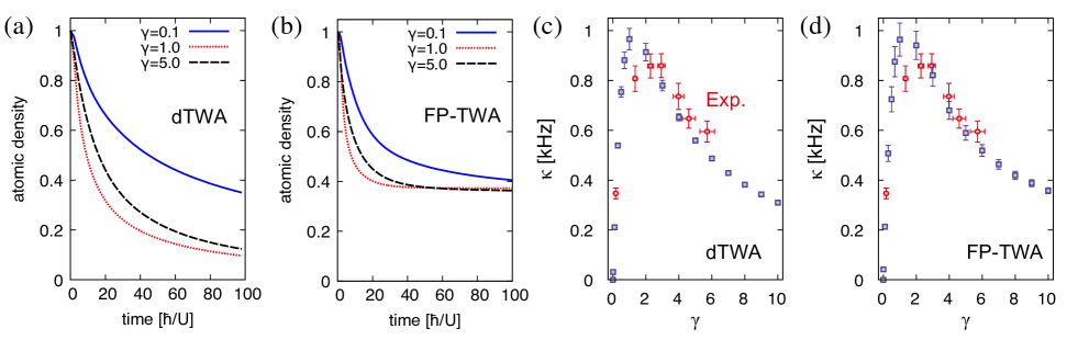
Figure 2: (a) SU(3) dTWA results for the non-unitary time evolution of the atomic density $n_{j}(t)$ starting from the unit filling Mott insulating state $|\psi_{\rm Mott}\rangle$ for three different values of the dissipation strength $\gamma=\hbar\Gamma_{\rm PA}/U$. The results for $\gamma=0.1$, $1.0$, and $5.0$ are shown by the blue solid, red dotted, black dashed lines, respectively. (b) Same as (a) but for SU(3) FP-TWA results. (c) Two-body loss rate $\kappa$ as a function of $\gamma$ (blue open squares) extracted from the dTWA results for $n_{j}(t)$ shown in (a). The error bar for each result denotes the standard estimation error for the fitting. We take the data points of the density $n_{j}(t)$ in (a) for the fitting such that the distance between adjacent points in the time axis is given by $\delta t_{\rm fit}=0.2\hbar/U$. (d) Same as (c) but for the SU(3) FP-TWA results. For comparison, the experimental results reported in Ref. Tomita et al. (2017) are also plotted by the red open circles in (c) and (d). Here in all calculations, we set the hopping amplitude $J=0.08U$.

In order to extract the two-body loss rate $\kappa$ from the behavior of the decay in $n_{j}(t)$, we utilize a fitting function with the form $f_{\kappa}(t)=(1+\kappa t)^{-1}$ for the early time regimes satisfying $n_{j}(t)>0.4$ Tomita et al. (2017). Note that this fitting function is the solution of a damping equation of the density associated with two-body losses, i.e., $\frac{dn_{j}}{dt}=-\kappa n^{2}_{j}$ with the initial conditions $n_{j}(t=0)=1$ Syassen et al. (2008). Figure 2(c) shows the loss rate $\kappa$ for the SU(3) dTWA as a function of $\gamma$. Note that $\gamma$ is independent of the optical lattice depth. Here we assume the recoil energy of the optical lattice $E_{\rm R}/\hbar\approx 2\pi\times 4.0$ kHz for the lattice depth $d_{\rm lat}=266$ nm. One of the main findings in Fig. 2(c) is the manifestation of the continuous quantum Zeno effect in the vicinity of $\gamma\sim 1$, which is qualitatively consistent with the experimental observation in Ref. Tomita et al. (2017). For more quantitative comparison, we also show in the same figure the corresponding experimental results and find that they are in good agreement with our theoretical results within the experimental errors. In the weak dissipation regime with $\gamma\lesssim 1$, the loss rate $\kappa$ becomes larger with increasing $\gamma$. As opposed to this behavior, in the strong dissipation regime with $\gamma\gtrsim 1$, the loss rate $\kappa$ decreases with increasing $\gamma$, which can be attributed to the suppression of double occupation of sites due to strong two-body losses, i.e., the Zeno effect Tomita et al. (2017).

We note that, in the setup of Ref. Tomita et al. (2017), the controllable range of $\gamma$ is limited to $0\leq\gamma\lesssim 5$. Our dTWA results strongly support that the continuous Zeno effect is much more enhanced when $\gamma$ is further raised above $\gamma=5$ beyond the experimentally accessible range. This is in accordance with the intuition anticipated for the Zeno effect and makes the experimental observation of the Zeno effect in Ref. Tomita et al. (2017) more substantial. Additionally, as shown in Fig. 2(d), the FP-TWA also produces a similar curve of $\kappa$ as a function of $\gamma$, implying almost the same threshold to the Zeno regime, but it has typically larger error bars in estimating the values due to the nonlinear properties of the Langevin equation.

Let us now discuss the qualitative difference between the two semiclassical descriptions by comparing these results. The onsite linearity of the dTWA leads to long-time behavior for $tU/\hbar\gtrsim 10$ that are qualitatively distinguishable from those in the FP-TWA. In particular, for the typical values of $\gamma$ in Fig. 2, the density $n_{j}(t)$ at, for example, $tU/\hbar=100$ in the dTWA significantly deviates from that in the FP-TWA, even though the short-time behavior agrees well for $tU/\hbar\lesssim 10$. Moreover, as shown in Fig. 2(b), $n_{j}(t)$ obtained by the FP-TWA for $\gamma=4$ and $5$ crosses at a certain time, while there is no such intersection found for the dTWA results in Fig. 2(a). In order to gain insight into the validity of the TWA descriptions, we will compare in Sec. IV.4 the semiclassical results for a small cluster with the numerically exact results of the master equation. There, we find that the long-time behavior obtained by the dTWA are qualitatively similar to those in the exact results, and that the FP-TWA is less qualitative than the dTWA due to the nonlinearity of the dissipative contribution. Therefore, we conclude that the dTWA results in Fig. 2 are more reliable.

IV.2 Linear sweep time sequence of the hopping

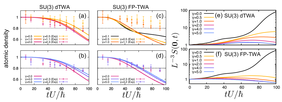
Figure 3: (a-b) SU(3) dTWA results of the non-unitary time evolution of the atomic density $n_{j}(t)$ for the atom loss dynamics at the unit filling Mott insulating state $|\psi_{\rm Mott}\rangle$ with the linear sweep time sequence crossing the ground state phase transition point of the Bose-Hubbard Hamiltonian, i.e., $J_{\rm ini}=0$ and $J_{\rm fin}=0.04U$. The values of the dissipation strength $\gamma$ are indicated in the figures. The time grid size for the Runge-Kutta scheme is set to be $\Delta t=2.0\times 10^{-3}$. (c-d) Same as (a-b) but for SU(3) FP-TWA results. Here, the time grid size for the Euler-Maruyama scheme is set to be $\Delta t=2.0\times 10^{-4}$. For comparison, the experimental results in Ref. Tomita et al. (2017) are also plotted by circles with error bars in (a)–(d). (e-f) Time evolution of the phase coherence extracted from the single particle correlation functions, i.e., $S({\bm{0}},t)$, for the linear sweep time sequence evaluated by (e) the SU(3) dTWA and (f) the SU(3) FP-TWA.

Next, we analyze how the two-body loss dissipation affects the coherent time evolution caused by a slow parameter change in the Hamiltonian. At zero temperature and for a commensurate mean filling, the Bose-Hubbard Hamiltonian $\hat{H}_{\rm BH}$ exhibits a second order quantum phase transition between a Mott insulating state and a superfluid state Fisher et al. (1989); Capogrosso-Sansone et al. (2007). In the three dimensional setup with the mean occupation tuned at unit filling, the phase transition occurs at $J_{\rm c}=0.0341U$. This exact critical value was numerically estimated in Ref. Capogrosso-Sansone et al. (2007) by employing a quantum Monte Carlo method. Note that the mean-field Gutzwiller approximation yields the critical point $J_{\rm c}^{\rm MFA}=0.0286U$ van Oosten et al. (2001), which is smaller than the exact value because of the less accuracy of the site decoupling approximation.

Here in our simulations, we prepare the unit filling Mott insulating state $|\psi_{\rm Mott}\rangle$ at $t=0$ and then slowly drives it with the Lindblad equation for a time-dependent hopping amplitude at a fixed value of $\gamma$. In order to realize a setup that is close to the real experiment, we assume a linear sweep time sequence of the hopping given by $J(t)=J_{\rm ini}+(J_{\rm fin}-J_{\rm ini})(t/\tau)$ for $0\leq t\leq\tau$ Tomita et al. (2017). $J_{\rm ini}$ and $J_{\rm fin}$ are the initial and final hopping amplitudes, which are set in the Mott insulating and superfluid sides, respectively. During this sweep, the onsite interaction strength $U$ remains constant. In the experiment reported in Ref. Tomita et al. (2017), the tuned parameter is the optical lattice depth and it is linearly ramped down from the Mott insulating regime to the superfluid regime. The dominant effect arising in the dynamics during the ramping down is the exponential increase of the hopping energy. Hence, the linear sweep time sequence of the hopping provides a reasonable simplification of the time sequence realized in the experiment.

Figures 3(a) and 3(b) show the SU(3) dTWA results of the atomic density $n_{j}(t)$ for the atom loss dynamics with the above time sequence of the hopping amplitude $J(t)$. We specifically choose $J_{\rm ini}=0$ and $J_{\rm fin}=0.04U$ such that $J_{\rm ini}<J_{\rm c}^{\rm MFA}<J_{\rm c}<J_{\rm fin}$ holds. The sweep time is taken to be $\tau=100\hbar/U$, for which non-adiabatic excitations of the system are sufficiently suppressed during the sweep. For the weak dissipation strength such as $\gamma=0.5$, the loss of atoms becomes significant at an onset time $tU/\hbar\sim 83.5$. Here, the onset time is defined as a time above which the atomic density is less than $0.8$, as indicated by a dotted line in Fig. 3(a). As shown in Fig. 3(a), the onset time shifts to an earlier time with further increasing $\gamma$ for $\gamma\lesssim 2$. Indeed, the onset times for $\gamma=1$ and $\gamma=2$ are $tU/\hbar\sim 73.9$ and $tU/\hbar\sim 71.1$, respectively. However, for the strong dissipation strength, i.e., $\gamma\gtrsim 2$, the onset time shifts to a later time with increasing $\gamma$, as shown in Fig. 3(b). This result manifests the continuous quantum Zeno effect in the sweep dynamics and a similar behavior has also been observed experimentally in Ref. Tomita et al. (2017). The threshold strength of $\gamma$ separating the Zeno and non-Zeno regimes is $\gamma\sim 2$, which also agrees well quantitatively with the experimental observation Tomita et al. (2017). Since the numerically exact result for a small cluster also supports a similar onset value, as demonstrated in Sec. IV.4, our result here is considered to be qualitatively reliable.

The SU(3) FP-TWA also describes the delay of the atomic loss in the sweep dynamics for the strong dissipation strength. However, it gives rise to a qualitatively different result, as shown in Figs. 3(c) and 3(d). Namely, in contrast to the dTWA result, the delay occurs already for $\gamma\gtrsim 0.1$, implying that the Zeno regime is broadened in the side of smaller $\gamma$. For instance, along the time slice at $t=40\hbar/U$ in Figs. 3(c) and 3(d), the atomic density is found to be significantly suppressed even for $\gamma=0.1$, and it starts to increase with further increasing $\gamma$ beyond the threshold. In other words, the nonlinearity of the FP-type approximation manifests itself in too much amount of suppression of the atomic density, and thus the Zeno regime is rather broadened within the SU(3) FP-TWA.

In Figs. 3(a)–3(d), we also plot the experimental results of the atomic density for $\gamma=0.5$, $1.1$, $2.3$, and $4.2$ reported in Ref. Tomita et al. (2017), which should be directly compared with our TWA results for $\gamma=0.5$, $1$, $2$, and $4$, respectively. Here, the experimental results are plotted along the time axis such that the values of $J/U$ during the sweep in the experiment are the same as the corresponding values in the linear sweep time sequence employed in our simulations. As shown in these figures, we find that, specifically in the SU(3) dTWA, the qualitative behavior of the $\gamma$ dependence of the melting dynamics is reasonably captured within the experimental error bars.

We further analyze the suppression of the superfluid phase coherence in the presence of the strong two-body loss dissipation. For this purpose, we consider a spatial Fourier transform of the equal-time single particle correlation function, i.e., the momentum distribution, defined by

$$S({\bf k},t)=\sum_{{\bf R}_{i},{\bf R}_{j}}e^{i{\bf k}\cdot({\bf R}_{i}-{\bf R}_{j})}{\rm Tr}\left[\hat{\rho}(t){\hat{a}}^{\dagger}_{i}{\hat{a}}_{j}\right],$$ (21)

where ${\bf R}_{i}$ represents the real space vector specifying site $i$ and ${\bf k}$ denotes the momentum vector in three dimensions. Note that this distribution is measurable in experiments by using the time-of-flight (TOF) imaging techniques Lewenstein et al. (2012). Here, we specifically set ${\bf k}=(0,0,0)$ for the purpose of quantifying the emergence of coherence over long distances after the hopping sweep. In addition, we note that no inhomogeneity effect due to a trapping potential for the gas is taken into account here.

Figure 3(e) shows the SU(3) dTWA results for $S({\bf 0},t)$. In the absence of dissipation, i.e., $\gamma=0$, the growth of long distance correlations is recovered within this approximation, implying a dynamical phase transition of the system from the Mott insulating phase to a superfluid phase. For the weak dissipation strength, i.e., $\gamma\leq 1$, this semiclassical method remains to produce large occupation of the zero momentum distribution at the final state, i.e., $L^{-3}S({\bf 0},t=\tau)\gg 1$. Hence, the phase coherence comprised of coherent bosons survives well against the weak dissipation. However, for the strong dissipation strength, i.e., $\gamma\gtrsim 2$, the distribution is found to be strongly suppressed such that $L^{-3}S({\bf 0},t=\tau)\sim 1$, implying that the strong dissipation stabilizes the Mott insulating state and leads to the delay of the evolution toward a superfluid phase due to the continuous Zeno effect. This result is consistent with the experimental observation in TOF absorption images Tomita et al. (2017), revealing that the phase coherence associated with superfluidity is suppressed by the strong dissipation.

On the other hand, the SU(3) FP-TWA gives rise to much stronger suppression of the phase coherence because of its nonlinearity in the dissipation force. For example, as shown in Fig. 3(f), $L^{-3}S({\bf 0},t=\tau)\sim 1$ is realized even for the weak dissipation strength such as $\gamma=0.5$. Moreover, for $\gamma\gtrsim 1$, the distribution at the final state is significantly suppressed, i.e., $L^{-3}S({\bf 0},t=\tau)\ll 1$, also implying the loss of phase coherence.

IV.3 Restored superfluid coherence after turning off the PA light

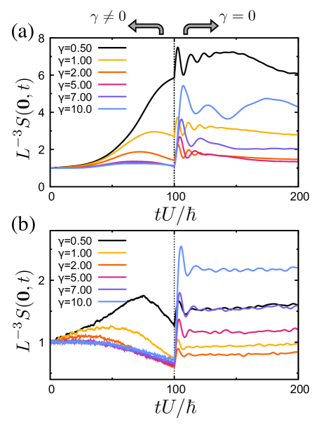
Figure 4: (a) SU(3) dTWA results for the non-unitary time evolution of the zero momentum distribution $S({\bf k}={\bf 0},t)$, where $\gamma$ varies from $\gamma\neq 0$ (indicated in the figure) to $\gamma=0$ at $t=\tau$, mimicking abrupt turning off of the PA light at $t=\tau$. For $t\leq\tau$, the linear sweep time sequence is applied, as in Fig. 3, while the hopping $J(t)=J_{\rm fin}$ for $t>\tau$. The vertical dotted line indicates the endpoint of the sweep at $t=\tau$. (b) Same as (a) but for SU(3) FP-TWA results.

Finally, we examine whether the SU(3) TWA can capture the restoration of the superfluid coherence after suddenly turning off the PA laser at $t=\tau$. A similar setup was implemented for the lattice ramp-down experiment in Ref. Tomita et al. (2017). It was observed in the experiment that after a certain hold time of the gas an interference pattern in TOF images is restored, implying the phase coherence reformation Tomita et al. (2017). This suggests that the suppression of superfluid coherence is not attributed to the heating caused by the PA laser and that the final state after the ramping down remains to be a Mott insulating state.

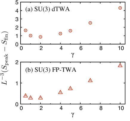
Figure 5: The restored peak height $\delta h=L^{-3}(S_{\rm peak}-S_{\rm fin})$ after turning off the PA laser, i.e., by setting $\gamma=0$ at the endpoint of the sweep (see Fig. 4), vs. the dissipation strength $\gamma$. The results are evaluated by (a) the SU(3) dTWA and (b) the SU(3) FP-TWA.

Figure 4 shows the SU(3) dTWA and FP-TWA results simulating the time evolution when $\gamma$ varies abruptly from $\gamma\neq 0$ to zero at $t=\tau$. We find that the increase of the zero momentum distribution occurs for each $\gamma$ after turning off the dissipation, implying the restoration of the phase coherence over long distances, as observed experimentally in the visibility measurements of TOF images Tomita et al. (2017). In the time region where $\gamma=0$, i.e., $t>\tau$, the momentum distribution at ${\bf k}={\bf 0}$ increases first up to a maximum peak, and then it eventually saturates afterward. Within the SU(3) TWA, the long time evolution for $t\gg\tau$ is expected to lead to a classical thermal state described by the Gibbs distribution for the classical chaotic Hamiltonian Wurtz et al. (2018), i.e., the SU(3) representation of the Bose-Hubbard model with a conserved filling factor.

In order to better characterize the properties of the restored peaks in the momentum distribution, let us define

$$S_{\rm peak}=\max_{t>\tau}[S({\bf k}={\bf 0},t)],\;\;S_{\rm fin}=S({\bf k}={\bf 0},t=\tau).$$

Figure 5 displays a restored peak height $\delta h=L^{-3}(S_{\rm peak}-S_{\rm fin})$ as a function of $\gamma$. In the SU(3) dTWA results shown in Fig. 5(a), the peak height $\delta h$ increases with increasing $\gamma$ for $\gamma\gtrsim 2$, while it decreases for $\gamma\lesssim 2$. The increase of $\delta h$ for $\gamma\gtrsim 2$ implies that much more particles stay in the system due to the stronger dissipation, i.e., the Zeno effect, before switching off the dissipation $\gamma$. Given the results in Figs. 3(a) and 3(b) on the atomic density in the linear sweep time sequence, the restored peak height $\delta h$ turns out to follow the total number of atoms surviving in the optical lattice at the end point of the sweep, i.e., $t=\tau$.

As shown in Fig. 5(b), a similar behavior of the $\gamma$ dependence of the peak height is also found in the SU(3) FP-TWA. Namely, $\delta h$ first decreases with increasing $\gamma$ and then starts to increase at a minimum point located around $1\leq\gamma\leq 2$. The presence of the minimum in this regime is also correlated to the behavior of the final state atom densities at $t=\tau$ shown in Figs. 3(c) and 3(d). However, we should note that the final states at $t=\tau$ are not reliable, even qualitatively, in the SU(3) FP-TWA, as implied by the numerically exact results in Sec. IV.4, and therefore we consult the SU(3) dTWA results to be compared with the experiment.

IV.4 Numerically exact results

Finally, we numerically examine the performance of the TWA schemes introduced here in this paper for the Lindblad master equation by comparing their results with the numerically exact ones.

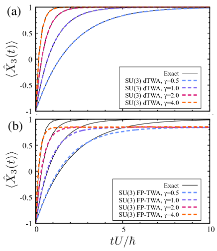
Figure 6: (a) Time evolution of $\langle X_{3}(t)\rangle$ for the single-site system with the two-body loss, corresponding to the $J=0$ limit of the dissipative Bose-Hubbard model, evaluated by the SU(3) dTWA. The initial state at $t=0$ is chosen to be the doubly occupied state $|2\rangle$. This state is the simultaneous eigenstate of ${\hat{X}}_{3}$ and ${\hat{X}}_{8}$, i.e., ${\hat{X}}_{3}|2\rangle=-|2\rangle$ and ${\hat{X}}_{8}|2\rangle=-\frac{1}{\sqrt{3}}|2\rangle$. Here, 1000 trajectories are used to obtain the smooth results as a function of time $t$. (b) Same as (a) but for the SU(3) FP-TWA results. Here, 100 000 trajectories are required to obtain the smooth results. For comparison, the exact solution of the master equation for each value of $\gamma$ is also provided by the solid line in (a) and (b).

In the case when the hopping amplitude is zero, i.e., $J=0$, the SU(3) dTWA reproduces the exact quantum time evolution generated by the master equation with a direct product state for the typical initial quantum state. This is attributed to the linearity of the classical equation of motion in the interaction $U$ term and the dissipation $\gamma$ term as implied in Eq. (10). Figure 6(a) displays numerical results calculated by the SU(3) dTWA for a single site system, demonstrating that this specific semiclassical representation successfully reproduces the exact solutions of the dynamics of $\langle{\hat{X}}_{3}(t)\rangle={\rm Tr}[\rho_{\rm eff}(t)T_{3}]$ for arbitrary dissipation strength at all time.

However, as shown in Fig. 6(b), the quantitative validity of the SU(3) FP-TWA is verified only within a finite timescale. This limitation is due to the nonlinearity in the dissipation term of the Langevin equation. For $\gamma=0.5$, the SU(3) FP-TWA simulation coincides well with the numerically exact solution until $tU/\hbar\sim 3$. After this timescale, the SU(3) FP-TWA result deviates from the numerically exact solution and finally flows to a false steady state with $\langle{\hat{X}}_{3}(t)\rangle<1$ for $tU/\hbar\gg 1$. Note that the exact steady state for the present setup is the trivial bosonic vacuum state $|0\rangle$, implying $\langle{\hat{X}}_{3}(t)\rangle=1$ for $tU/\hbar\gg 1$. For larger values of $\gamma$, i.e., $\gamma=1$, $2$, and $4$, the threshold time is estimated as $tU/\hbar\sim 1.5$, $1$, and $0.5$, respectively. Hence, the valid timescale of this approximation is shortened with increasing $\gamma$. Notice also that the time evolved states for these different values of $\gamma$ result in the same false steady state at long time. Comparing the results in Figs. 6(a) and  6(b), the local linearity of the dissipative force in the SU(3) dTWA is essential to reproduce the correct steady state reached via the successive onsite losses in time.

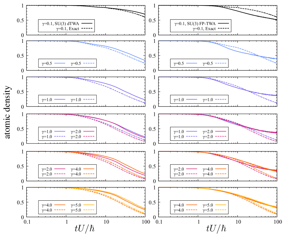
Figure 7: The SU(3) dTWA (left panels) and the FP-TWA (right panels) results of the non-unitary time evolution of the atomic density $n_{j}(t)$ for the dissipative Bose-Hubbard model on a four site ring (solid lines). The initial state at $t=0$ for the time evolution is the unit filling Mott insulating state $|\psi_{\rm Mott}\rangle$. The hopping amplitude $J$ is the same as in Fig. 2, i.e., $J=0.08U$, and the values of the dissipation strength $\gamma$ are indicated in the figures. For comparison, the numerically exact solutions are also plotted by dashed lines. In the SU(3) dTWA, the time grid size for the explicit fourth-order Runge-Kutta scheme is set to be $\Delta t=2.0\times 10^{-2}$ and the number of generated classical trajectories is $20\;000$. In the SU(3) FP-TWA, the grid size for the first-order Euler-Maruyama scheme is set to be $\Delta t=2.0\times 10^{-4}$ and the number of generated Langevin trajectories is $200\;000$.

We further examine how well the semiclassical representations can reproduce the exact solutions of the master equation in a multiple site case with a nonzero hopping. For this purpose, let us consider a chain composed of $L=4$ sites under periodic boundary conditions. Except for the spatial geometry of the system, the situation considered here is the same as that in Sec. IV.1. Namely, starting from the Mott-insulating state $|\psi_{\rm Mott}\rangle$ at unit filling, we suddenly turn on the dissipation $\gamma$ as well as the hopping $J$ at $t=0$ and numerically calculate the time evolution of the atomic density $n_{j}(t)$, where we choose $J=0.08U$.

The left panels of Fig. 7 compare the SU(3) dTWA results of the atomic density $n_{j}(t)$ with the numerically exact solutions for different values of $\gamma$. For $\gamma=0.1$, the result obtained by the SU(3) dTWA agrees very well with the exact solution until $tU/\hbar\sim 10$, but is merely qualitative at later time, where the deviation becomes larger as the time further evolves. However, for $\gamma\gtrsim 0.5$, the time regime in which the SU(3) dTWA description is quantitative is shortened up to $tU/\hbar\sim 1$. This is due to the approximate treatment of the offsite hopping term in the Bose-Hubbard Hamiltonian. In other words, the SU(3) dTWA cannot quantitatively evaluate the dynamical creation of double occupation per site at long time, which occurs via tunnelings of the atoms between sites. Regardless of such a limitation, it is noteworthy that the SU(3) dTWA can estimate a reasonable Zeno threshold value as compared to the exact dynamics, i.e., the delay of atom loss happens around $\gamma\sim 2$ in this one-dimensional system. Note also that the SU(3) dTWA results are always larger than the corresponding exact solutions, implying that higher order quantum corrections associated with offsite correlations give rise to the reduction of the atomic densities at all time.

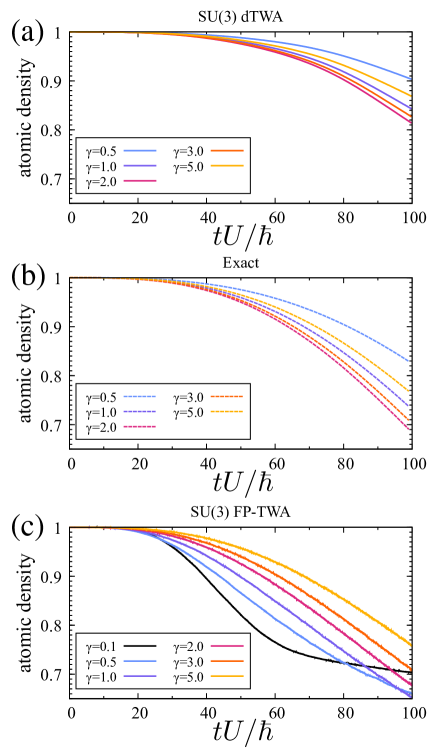
Figure 8: (a) Same as Figs. 3(a) and 3(b) but for a four site ring. The number of generated classical trajectories is $20\;000$. (b) Same as (a) but for the numerically exact solutions. (c) Same as (a) but for the SU(3) FP-TWA results. The number of the generated Langevin trajectories is $200\;000$.

The right panels of Fig. 7 show the SU(3) FP-TWA results of the atomic density $n_{j}(t)$ compared with the numerically exact solutions. For the weak dissipation strength, i.e., $\gamma=0.1$, the SU(3) FP-TWA result deviates form the exact solution around $tU/\hbar=2$. However, for the strong dissipation strength such as $\gamma=4$ and $5$, the SU(3) FP-TWA and exact results coincide rather well until $tU/\hbar\lesssim 6$. We should note that this coincidence is not controlled in this approximation. Although the SU(3) FP-TWA can capture the continuous Zeno effect for the strong dissipation strength, it estimates the threshold at $\gamma\sim 1$, which is smaller than the exact solution. Comparing the SU(3) dTWA and FP-TWA results, we conclude that the qualitative performance of the SU(3) FP-TWA is worse than that of the SU(3) dTWA at long time.

We also evaluate the performance of these semiclassical methods in the case of the time dependent linear sweep of the hopping amplitude discussed in Sec. IV.2. As shown in Fig. 8(a), the onset of the Zeno effect estimated by the SU(3) dTWA is around $\gamma\sim 2$, which is consistent with the numerically exact result shown in Fig. 8(b). However, as shown in Fig. 8(c), the FP-TWA estimates a wrong onset at $\gamma\sim 0.1$. Note that similarly a rather small onset of the Zeno effect is found in the three dimensional FP-TWA simulations in Fig. 3(c). As already discussed in Fig. 7, we also note that higher order corrections beyond the SU(3) dTWA reduce the atomic densities at all time for any $\gamma$. Finally, we should emphasize that although the qualitative behavior of the decay of the atomic density in the SU(3) dTWA is similar to that in the exact dynamics, apart from the systematic corrections with the same sign, the FP-TWA fails to capture even such qualitative behavior.

V Conclusions

In conclusions, we have generalized the SU(3) TWA method for the Bose-Hubbard system to the Lindblad dynamics in the presence of onsite dissipation terms. We have presented two semiclassical representations of the dynamics governed by the effective Lindblad master equation, namely the discrete TWA representation and the Fokker-Planck TWA representation. The two methods have been applied to the dissipative Bose-Hubbard system with the two-body losses, which has been previously addressed experimentally in Ref. Tomita et al. (2017). It has been demonstrated that these semiclassical representations can qualitatively capture the essential features of the continuous quantum Zeno effect in the dissipative non-unitary dynamics, as observed experimentally. In particular, the discrete TWA representation is found to produce reasonable thresholds of the dissipation strength separating between the Zeno and non-Zeno regimes, which are comparable to the experimental results of the analog quantum simulation Tomita et al. (2017). This is attributed to the onsite linearity of the classical equation of motion in the discrete TWA representation, which is to be used in the Monte Carlo simulations.

As a future study, it is interesting to apply these SU(3) TWA methods introduced here to other experiments associated with dissipative Bose-Hubbard systems Labouvie et al. (2016); Bouganne et al. (2020) and discuss the reproducibility of nontrivial driven-dissipative dynamical phenomena reported there. It is also interesting to improve the semiclassical methods based on onsite variables by using the cluster TWA method Wurtz et al. (2018) in order to treat more accurately offsite quantum correlations caused by the hopping term.