Coexisting periodic attractors
under the influence of noise in injected photonic oscillators

Abstract

The optical power spectrum is the prime observable to dissect, understand and design the long-time behavior of arrays of optically coupled semiconductor lasers. A long-standing issue has been identified within the literature on injection locking: how the thickness of linewidth and the lineshape waveform envelope correlates with the deterministic evolution of the slave laser oscillator and how the presence of noise and the dense proximity of coexisting limit cycles are shaping and influencing the overall spectral behavior. In addition we are critically interested in the regions where the basin of attraction has self-similar and fractal-like behavior, still, the long-time orbits are limit cycles, in this case, period-one (P1) and period-three (P3). Via numerical work, we find that the overall optical power spectrum is deeply imprinted with a strong influence from the underlying noise when the system lives in the region of the P1 and P3 limit cycles. Additionally, a qualitative comparison is made between the stochastic Langevin simulations and the recorded optical power spectra taken from older experiments that we revisit. Finally, we point to a possible set of next-generation applications in photonics and quantum technologies where such findings may have substantial implications.

I Introduction

An attractor of a dynamical system is a subset of the state space where the orbits originating from typical initial conditions tend as time evolves. It is a rather common feature for nonlinear dynamical systems to have multiple attractors. For each such dynamical state, its basin of attraction is the set of initial conditions that eventually lead to it. As a result, the qualitative behavior of the long-time evolution of a given system can be radically different depending on which basin of attraction the initial condition resides in.

To the best of our knowledge, there have been very few experimental in-depth studies of basins of attraction because following the evolution of initial conditions in low-frequency macroscopic systems is usually very time-consuming and system parameters tend to drift over the course of many data recording runs Roukes2007 . Fractal basin boundaries MCD85 , in particular, have been found numerically and investigated experimentally in man-made systems where the key oscillating frequency is rather slow.

A system that is of significant technological relevance and is well-known for demonstrating multiple attractor behavior is the optically injected laser. The complexity of this system involves a rich set of qualitatively different dynamical features, including stable and unstable steady states (fixed points) and self-sustained oscillations (limit cycles), as well as self-modulated quasiperiodic (tori) and chaotic orbits (strange attractors) ERN10 ; OHT13 ; WIE05 . The long-term dynamics of the injection-locking architecture enabled with semiconductor lasers, such as quantum well, quantum dot, and quantum cascade lasers on photonic integrated circuits or on a tabletop configuration with discrete devices has been investigated analytically, numerically, and experimentally for the past 50 years Costas2020 .

The speed of the free-running relaxation oscillation of these tunable photonic oscillators typically starts at a few GHz and may cross 84 GHz under strong injection and for large optical frequency detuning Herrera2021 . Therefore the mapping of the basins of attraction in such a system of ultra fast oscillators can be explored only numerically. Examples of such explorations and fine detailed numerical scans on regions of chaos and period 3 limit cycle orbits laying within the chaotic orbits, were reported for zero optical detuning in Jason2010 .

Semiconductor lasers are known to have a high level of intrinsic noise primarily due to spontaneous emission Agrawal90 which broadens and obscures their spectral properties. From a dynamical point of view such fluctuations may lead to noise-induced attractor switching and therefore affect the output waveform. Self-sustained oscillators that support robust limit cycles have a major technological significance with devices that generate periodic signals at an inherent frequency and are often engineered to enable highly accurate time or frequency references. Therefore it is of high importance to map out the dynamical regimes of such states and study how stochastic fluctuations interact with their basins of attraction. The prime observable through which these phenomena can be analyzed is the optical power spectrum.

One of the key technical issues that we are working forward to is to address the spectrum congestion and demand for higher data rates that are driving a push toward higher carrier frequencies in wireless communications, necessitating sources of exceptionally pure widely tunable radiofrequency carrier signals. Multiple applications may be influenced such as laser radar applications, optical metrology, and spectroscopy. It is worth noting that pivotal issues of current applications of quantum sensing are deeply dependent on the use of properly sharp linewidth as well as wide frequency tunable oscillators QuantumGYRO2023 and a range of geolocation applications SPIE2023 .

This paper is organized as follows: after the introductory section, the single-mode optical injection rate equation system is presented with noise terms incorporated. Next, we perform a detailed analysis of the deterministic dynamics in the regime of interest where the system’s behavior is dominated by the coexistence of four-wave mixing and period-three limit cycles. The corresponding basins of attraction are computed and their fractal-like structure is noted. The following section focuses on the optical power spectra corresponding to the observed dynamics, while the interplay of noise and the fractal-like basins of attraction and its imprint on the spectral properties of the emitted signal is discussed. In the conclusions we summarize our main findings and propose new directions for further studies.

II Injected Photonic Oscillator Model

The dynamic time evolution of an optically injected semiconductor laser subject to an externally imposed monochromatic signal is modeled, in dimensionless form, by three single-mode rate equations, one covering the dynamics of the amplitude $R$ of the electric field emitted out of the slave cavity, one for the phase offset $\phi$ between the two lasers, and one for the electronic carrier density into the nonlinear gain medium of the slave laser cavity, $N$:

$$\frac{dR}{dt} = NR+\eta\cos\phi+F_{a}$$ (1)

$$\frac{d\phi}{dt} = \Omega-\alpha N-\frac{\eta}{R}\sin\phi+\frac{F_{p}}{R}$$ (2)

$$T\frac{dN}{dt} = P-N-P(1+2N)R^{2}.$$ (3)

In the above system, $\eta$ is proportional to the amplitude of the externally injected field, $\Omega$ is the optical frequency detuning between the slave and master emission optical frequencies, $\alpha$ is the linewidth enhancement factor, $T$ is the ratio of the carrier to the photon lifetimes, $P$ denotes the electronic pumping current above the solitary laser threshold, and $t$ is the time normalized to the photon lifetime. In addition, fluctuations for the amplitude and the phase that the optical gain medium is generating into the slave cavity are incorporated. These fluctuations are represented by the Langevin noise sources $F_{a}(t)$ and $F_{p}(t)$, respectively. They are zero-mean, $\langle F_{i}(t)\rangle=0$, delta-correlated, $\langle F_{i}(t)F_{j}(t^{\prime})\rangle=D\delta_{ij}\delta(t-t^{\prime})$ ($(i,j=a,p)$) and $D$ is the noise intensity, proportional to the spontaneous emission rate PhysicsLetters1998 .

This set of three equations collects and fuses intelligently all the key features of the optical gain of the slave laser cavity and the stochastic dynamics of the optically injected laser, bringing into focus the two-time scales of the electrons (nanoseconds) and the photons (picoseconds), the strong phase-to-amplitude coupling via the linewidth enhancement factor, and the noise that drives and promotes the free-running relaxation oscillation sidebands of the slave laser Vahala1983

This unusually simple-looking rate equation model is well-established and has been the subject of investigations for more than five decades. It has been used to examine the bifurcation structure WIE05 , design multiple laser experiments on tabletop and chip scale configurations, and for spinning out a whole host of microwave photonic applications including wide-frequency tunable photonic oscillators Herrera2021 , bandwidth-enhancing emitters simpson1995 , and low-noise microwave oscillators Simpson2014 . Also, it has provided a framework for generating novel quantum states such as squeezed quantum mechanical states for injecting quantum light into interferometers, and laser ring gyros, and establishing next-generation phase modulators for hacking secure quantum key distribution communication links Yamamoto1 ; Yamamoto2 ; Yamamoto3 ; Yamamoto4 . In addition, recently, the strong four-wave mixing properties of the frequency tunable limit cycle were used as the “fictitious” four wave mixing medium for the generation of time crystals and optical frequency combs HIM23 .

III Coexisting Limit Cycles and their Fractal-Like Basin of Attraction

In this section, we focus on the deterministic behavior of the system in a specific dynamical regime that presents particularly interesting features. This regime corresponds to a finite, constant optical detuning expressed by the parameter $\Delta=\Omega/\omega_{r}$, where $\omega_{r}$ is the free-running angular relaxation frequency, which to a good approximation is equal to $\sqrt{2P/T}$ Herrera2021 .

We numerically integrate Eqs. (1-3) for $D=0.0$ in time using a standard fourth-order Runge-Kutta algorithm. Figure 1 depicts an orbit diagram that captures the rich complexity of the injection locking architecture for the specific choice of the detuning. In particular, we have plotted the extrema of the amplitude of the electric field in dependence of the injection strength $\eta$. Starting at $\eta=0.2$ where the only solution is a stable fixed point, the system, as $\eta$ decreases, undergoes a Hopf bifurcation at $\eta=0.167$ and a stable limit cycle is born. This is a well-known dynamical scenario of the optically injected laser model that has been extensively studied and experimentally confirmed in multiple types of laser oscillators, including quantum well and quantum dot lasers simpson1995 and recently quantum cascade oscillators wang2023 . In a series of papers in the 1990s, we recorded multiple transitions into chaos and coherence collapse states and performed a set of original stochastic and deterministic computations to prove the interplay of stochasticity and nonlinearity simpson1995 .

As $\eta$ decreases, a new periodic orbit is born, namely, a period-3 limit cycle as we discuss next, through a saddle-node (fold) bifurcation of limit cycles. This occurs at two values of the injection strength, $\eta=0.04$ and $\eta=0.00218$, while for intermediate values of $\eta$ these limit cycles undergo period-doubling bifurcations leading to a narrow chaotic region. A detailed bifurcation diagram showing the aforementioned bifurcation lines in the $(\Delta,\eta)$ parameter space is shown in Fig. 2 MATCONT .

Our focus of interest here are two regions for the injection strength ($\eta=0.008$ and $\eta=0.035$), marked by the vertical red lines in Fig. (2) and blown-up in Figs. 1(b) and (c), where two periodic limit cycles coexist. Specifically, a lower amplitude period-1 (P1) or four-wave mixing (FWM) limit cycle coexists with a higher amplitude period-3 (P3) limit cycle, born through a fold bifurcation. The time series of the electric field amplitude (left panel) and phase portraits (right panel) of these orbits are shown in Figs. (3) and (3) for $\eta=0.008$ and $\eta=0.035$ in (a) and (b), respectively. For the weal injection case ($\eta=0.008$), notice that compared to the P1 orbit (orange, light), the P3 limit cycle (blue, dark) is about three times larger in oscillation amplitude and occupies a larger region of the phase space $(R,N)$.

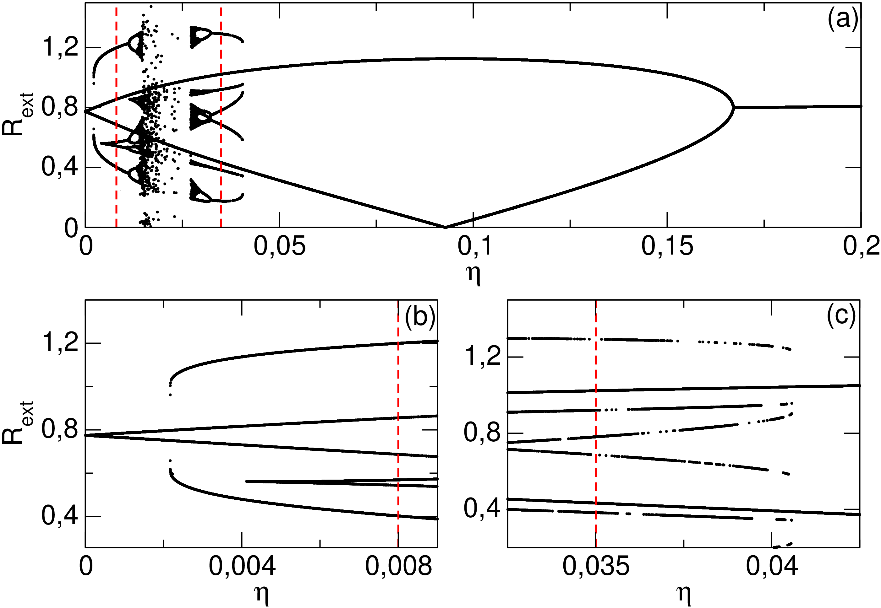
Figure 1: (a) Orbit diagram showing the extrema of the electric field amplitude for varying injection strength $\eta$, obtained by numerically integrating the rate equations Eqs. (1-3) for the following parameter values: $T=1000$, $\alpha=6$, $P=0.6$, and $\Delta=3$. Panels (b) and (c) show blow-ups around $\eta=0.008$ and $0.035$, respectively, marked by the vertical red dashed lines.

Figure 2: Bifurcation lines obtained by a numerical continuation of Eqs. (1-3) in the $(\Delta,\eta)$ parameter plane. “H” marks the Hopf bifurcation, “F” the fold (saddle-node) bifurcation of limit cycles, and ‘PD” the period-doubling bifurcation. Other parameter values are kept fixed to: $T=1000$, $\alpha=6$, $P=0.6$.

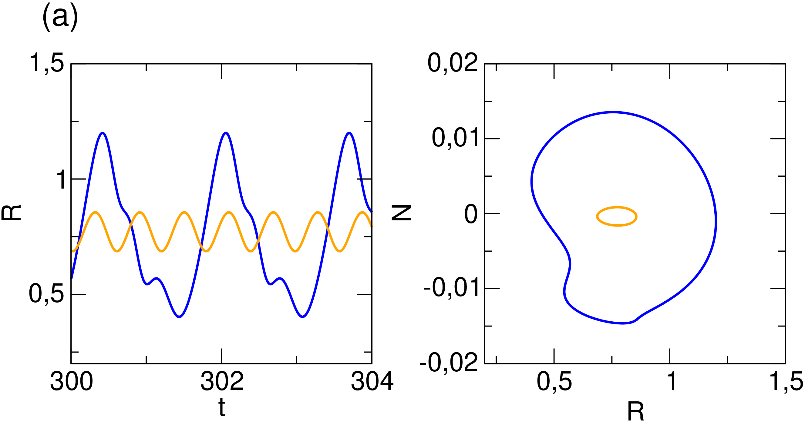
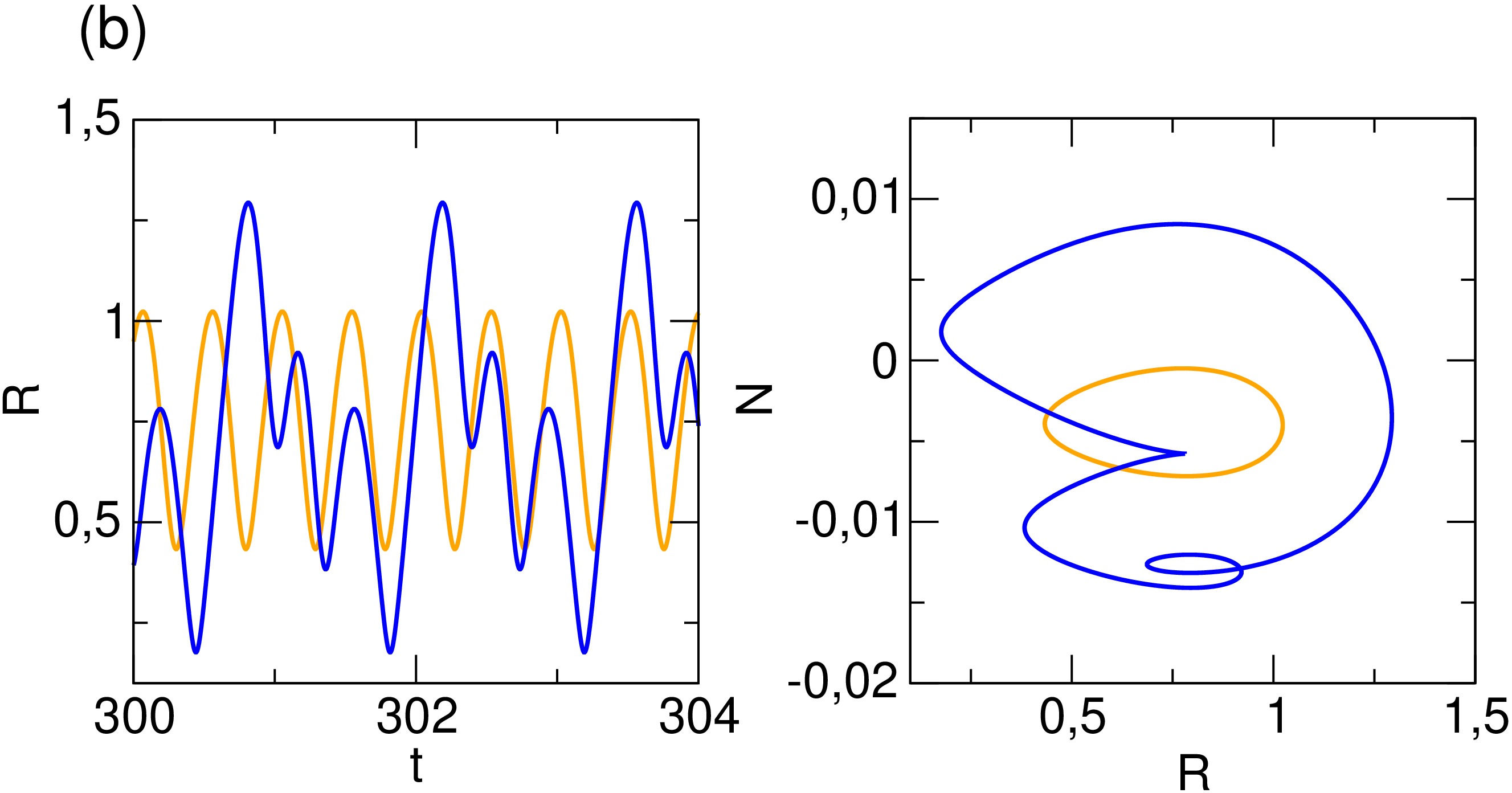
Figure 3: Deterministic time series of the electric field amplitude (left) and phase portraits in the $(R,N)$ plane (right) of the two limit cycles coexisting for a value of the injection rate (a) $\eta=0.008$ and (b) $0.035$, marked by the vertical red dashed lines in Fig. 1. Blue (dark) color corresponds to the period-3 solution and orange (light) color to the FWM (P1) solution. Other parameter values: $T=1000$, $\alpha=6$, $P=0.6$, $\Delta=3$, and $D=0.0$.

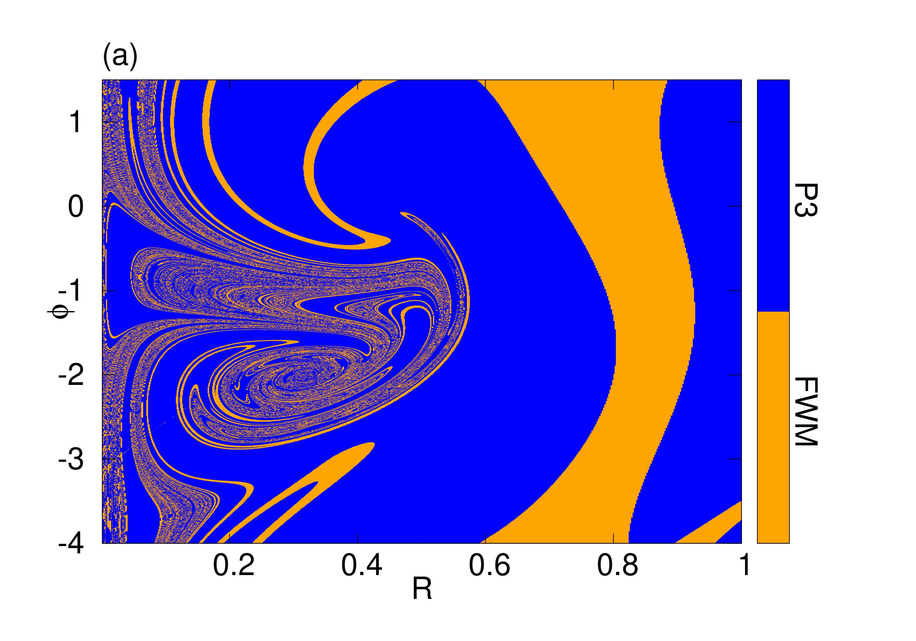
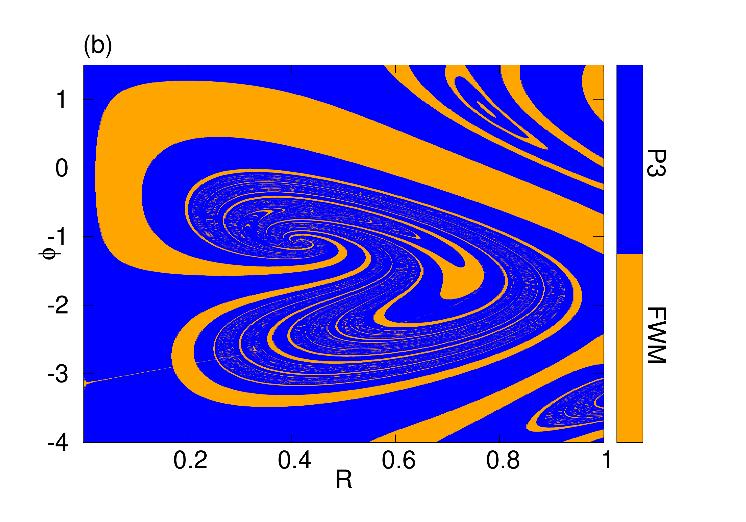
Figure 4: Basins of attraction in the $(R,\phi)$ plane for two values of injection strength (a) $\eta=0.008$ and (b) $0.035$. The initial condition for $N$ is set to zero. Blue (dark) color marks the initial conditions leading to a period-3 solution and orange (light) color marks the initial conditions leading to the coexisting FWM (period-1) solution. Other parameter values are: $T=1000$, $\alpha=6$, $P=0.6$, $\Delta=3$, and $D=0.0$.

.

The multistability exhibited by the model naturally renders it very sensitive to the choice of initial conditions. In order to illustrate this sensitivity, we have identified the basins of attraction of period-1 and period-3 oscillatory behavior for both values of the injection strength. These are displayed in Figs. 4 and  4, respectively, in the $(R,\phi)$ plane. Blue (dark) regions denote the set of initial conditions $(R(0),\phi(0))$ leading to P3 oscillations, while orange (light) regions are the ones leading to period-1 (FWM) oscillations. The other state variable is initially fixed to zero, $N(t=0)=0.0$. In both Fig. 4 and Fig. 4, it is observed that the sets of initial conditions leading to the P3 solution constitute a substantial part of the $(R,\phi)$ plane as indicated by the area occupied by the blue (dark) regions. Overall, the basins show a fractal-like composition as two long-time behavior of the limit cycles are mixed and intertwined. This behavior is similar to the P3/chaos region that has been found numerically for zero frequency optical detuning Jason2010 , with a key difference: in the latter, the system was lockedm while in this case the system is operating in an un-locked FWM region coexisting for large regions of the injection rate with a P3 orbit born out of a saddle mode bifurcation.

The knowledge of the basins of attraction of coexisting states is essential for determining the usefulness of the system in practical applications. For example, switching between outputs with different intensities and spectral properties may be utilized in optical communications LIU20 . In the following section, we study the effect of noise on the spectral linewidth and lineshape of the two coexisting limit cycles and the respective implications of the numerically found fractality in their basins of attraction.

IV Optical power spectra and the effect of noise

The Optical Power Spectrum has been the prime observable to dissect, understand and design the long-time behavior of optically coupled lasers. This fundamental quantity combines the amplitude and phase fluctuations of the recorded radiation emitted out of the slave laser cavity, where the noise of the laser amplifying medium as well as the nonlinear optical gain are encoded in the output radiation. Its numerical calculation is done based on the Fourier transform of the electric field $E(t)$, given by:

$$S(\omega)=\left|\int_{-\infty}^{+\infty}R(t)e^{i\phi(t)}e^{i\Omega t}e^{-i\omega t}dt\right|^{2}.$$ (4)

The deterministic power spectra (normalized to their maximum value) of the coexisting FWM (top panel, orange) and P3 (bottom panel, blue) orbits are depicted in Fig. 5 for both values of the injection strength, (a) $\eta=0.008$ and (b) $\eta=0.035$. As we anticipate, in the case of the period-1 limit cycle, apart from the power concentration around $\omega=0$, there is a prominent peak at the injected frequency $\omega=\Delta\omega_{r}$ ($\Delta=3$). On the other hand, in the case of the P3 limit cycle, we observe strong power concentrations at integer multiples of the free-running relaxation frequency $\omega_{r}$. Moreover, the linewidth of its center line is sharper than that of the corresponding FWM spectrum.

The basins of attraction serve as a guideline for obtaining the FWM or P3 spectrum on demand. However, in real-world conditions, noise is always present. The key question here is how noise affects the linewidth and the lineshape of two coexisting periodic limit cycles and what is the role of the numerically found fractality in their basins of attraction. We typically estimate the value of the noise intensity $D$ by connecting it with the linewidth of the center line of the FWM optical power spectrum and keep this value fixed to $0.001$ across all stochastic numerical simulations.

The stochastic differential equations are integrated numerically by applying Milstein’s method TOR14 which is suitable for systems that are driven by both additive and multiplicative noise terms in this case in the amplitude and phase variable of Eqs. (1) and (2) , respectively. The addition of noise helps the system alternate between period-1 and period-3 oscillatory motion, depending on the initial condition imposed by the random seed of each realization.

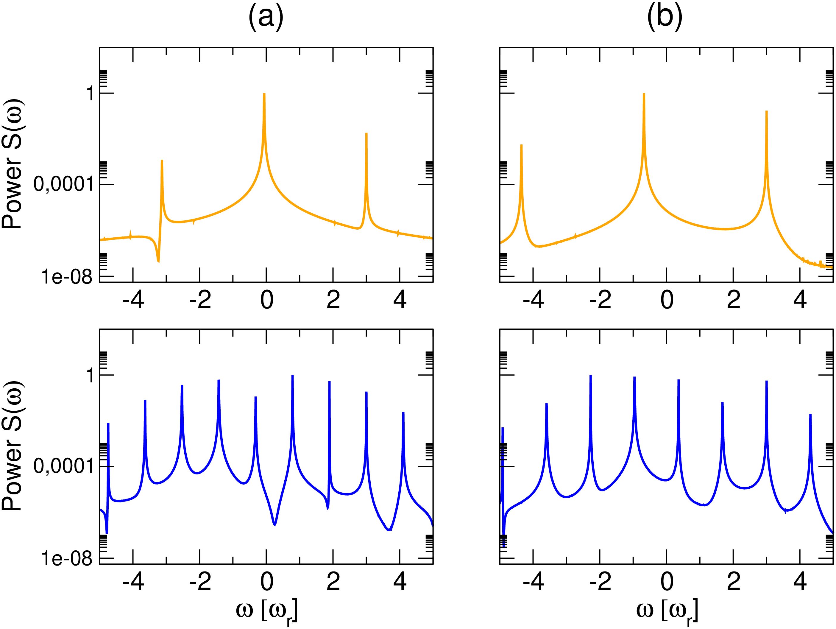
Figure 5: Deterministic optical power spectra for (a) $\eta=0.008$ and (b) $\eta=0.035$. Blue (dark) color corresponds to the optical power spectrum of the period-3 solution (P3) and orange (light) color to the optical power spectrum of the coexisting period-1 (FWM) solution. Other parameter values are: $T=1000$, $\alpha=6$, $P=0.6$, $\Delta=3$, and $D=0.0$.

In order to obtain a statistical average we executed 1000 noisy realizations for the two injection strength $\eta$ values. For $\eta=0.008$ all realizations land on the P3 periodic orbit, many after a very long transient time has elapsed. For $\eta=0.035$ about $35\%$ land on the P3 orbit, and the rest prefer the FWM orbit. Therefore we can conclude that noise favors absolutely the P3 orbit for weaker injection strength $\eta=0.008$, whereas for $\eta=0.035$ it prefers the FWM orbit. The corresponding noisy phase portraits are shown in Fig. 6 in green color, while the deterministic FWM and P3 orbits are also plotted on top for comparison.

Figure 6: Noisy (green) phase portraits in the $(R,N)$ plane for injection rate (a) $\eta=0.008$ and (b) $\eta=0.035$. The corresponding deterministic orbits are plotted on top: Blue (dark) color marks the P3 solution and the orange (light) color marks the FWM solution. Other parameter values are: $T=1000$, $\alpha=6$, $P=0.6$, $\Delta=3$, and $D=0.001$.

Next, we calculate the average spectrum over 100 noise realizations (each with a different random initial condition) comprising 1000 periods in total. These are plotted in Fig. (7), where the deterministic spectra are superimposed (and vertically shifted for visualization purposes), for the sake of comparison.

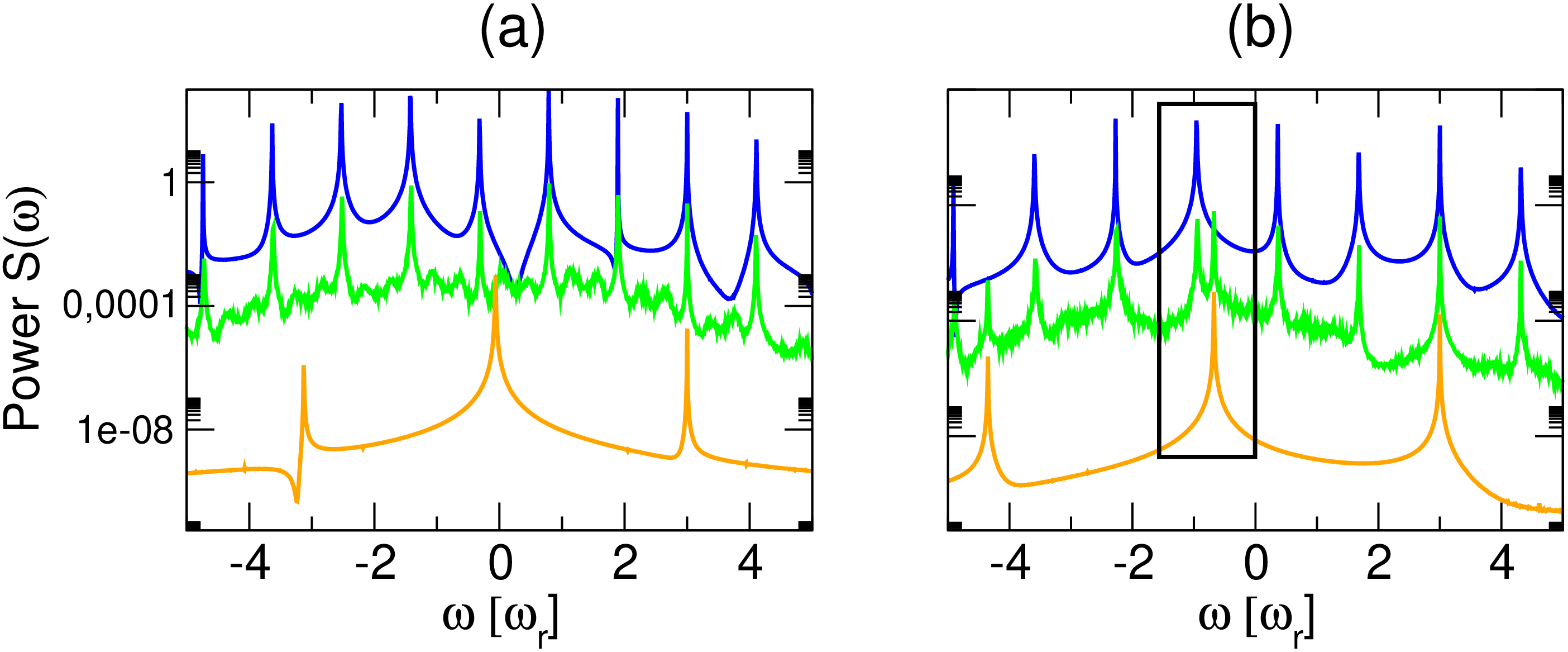
Figure 7: Noisy optical power spectrum for injection rate (a) $\eta=0.008$ and (b) $\eta=0.035$. The deterministic optical power spectra are included for comparison (shifted, for visualization purposes): Blue (dark) color marks the optical power spectrum of the P3 solution and the orange (light) color marks the optical power spectrum of the FWM solution. Other parameter values are: $T=1000$, $\alpha=6$, $P=0.6$, $\Delta=3$, and $D=0.001$.

For $\eta=0.008$ (Fig. 7 (a)), the noisy spectrum is similar to the noise-free P3 (blue, dark) spectrum since, as we discussed above, for weak injection strength noise favors this solution. Naturally, the primary spectrum peaks are thicker, and in addition, secondary smaller ones appear in between, due to the small fluctuations of the noise source. This was partly captured by the experimental measurement revisited in the Appendix, however, in that work, the optical power spectrum of the FWM signal was also recorded. The latter is predicted by our simulations too, but only as a very long transient phenomenon. On the other hand for $\eta=0.035$, the noisy spectrum reveals the primary peaks of both the FWM (orange, light) and the P3 (blue, dark) solution, marked by the black rectangle in Fig. 7 (b). This “mixed” spectrum image reflects the coexistence of the two orbits which for higher injection strengths persists, despite the fluctuations. This is a very interesting feature that was not observed in the reference experiment described in the Appendix which is definitely worth further investigation in a laboratory setting.

V Conclusions and Future Work

In this manuscript, we have systematically dissected the FWM and P3 region in the vicinity of optical detuning $\Delta=3$ for a wide region of the injection rate of the master laser. We find numerically two coexisting limit cycles one oscillating with period one and another oscillating with period three. At weak injection strengths, the period three limit cycle packs more intensity and is significantly more attracting than the period one solution. Deep numerical scanning of the basin of attraction of these two limit cycles reveals that the phase space has fractal features, making the system unpredictable and posing novel questions about the shape and the thickness of the linewidth of such emitted radiation where, in the presence of noise, the signal is a combination and/or fusion of the two outcomes. In future studies, we intend to further investigate such types of questions on the interplay of fractality and noise on the long-time optical spectra as well as how to engineer the basins and the strength of the noise to shape the spectral emission for a useful set of applications, such as coherent LIDAR, optical metrology and spectroscopy, and interferometric optical sensing. It is to be noted that key issues of current applications of quantum sensing are deeply dependent on the use of properly sharp RF linewidth as well as wide frequency low noise tunable photonic oscillators.

Acknowledgements

The VK research portfolio is supported via a VT Innovation Campus start-up, VT National Security Start-up, and generous gifts from private corporations including IDQ from Geneva to the Virginia Tech Foundation.

*

Appendix A

The work that motivated our study appeared in a book of abstracts of the annual Optical Society of America Conference in 1996 in Anaheim California Varangis1996 , as a rudimentary report on the combined theoretical and experimental study of the coexisting FWM and P3 limit cycles in the dynamical regime of optical detuning $\Delta=3$. Here, we briefly revisit the experimental setup and the main findings which are compared to the results of the present manuscript, in detail, in the main text.

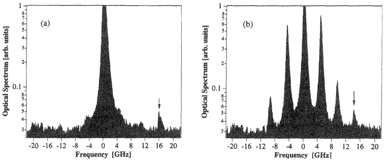
Figure 8: Experimentally recorded optical power spectra of an optically injected quantum well laser of HLP400 type, They were recorded by the scanning of the Fabry-Perot interferometer. The zero frequency in this figure is taken at the shifted center line. The master injection laser line is on the right marked by an arrow (positive detuning): (a) the FWM signal and (b) the P3 signal. Taken from Varangis1996

.

The experimental setup used in Varangis1996 consisted of two single longitudinal mode quantum well lasers, serving as master and slave, of HLP1400 type, emitting at a wavelength of 830 nm. The laser bars were temperature and current-stabilized and an optical isolator was used to prevent mutual light injection between the master and the slave elements. The radiation output of the lasers was monitored with the use of a Newport SR-240 scanning Fabry-Perot interferometer having a free spectral range (FSR) of 8 THz and linewidth resolution of 0.8 GHz. In Fig. 8 (respectively Fig. 2 in Varangis1996 ) we observe a typical four-wave mixing signal consisting of three emission lines: the slave center line, the four-wave mixing signal, and the regenerative line at the injected frequency. In Fig. 8 (b) we see in addition the appearance of a set of strong side bands at approximately 1/3 $f_{inj}$ and 2/3 $f_{inj}$. These sidebands are the manifestation of the period three isolated period solution, coexisting with the P1 signal.

References

- (1) I. Kozinsky, H. C. Postma, O. Kogan, A. Husain, and M. L. Roukes,Basins of attraction of a nonlinear nanomechanical resonator, Physical Review Letters 99, 207201 (2007).
- (2) W. McDonald, C. Grebogi, E. Ott, and J. A. Yorke, Fractal Basin Boundaries, Physica D 17, 125 (1985).
- (3) T. Erneux and P. Glorieux, Laser Dynamics, Cambridge University Press, Cambridge (2010).
- (4) J. Ohtsubo, Semiconductor Lasers: Stability, Instability and Chaos, Springer Series in Optical Sciences, Berlin (2013).
- (5) S. Wieczorek, B. Krauskopf, T.B. Simpson, and D. Lenstra, The dynamical complexity of optically injected semiconductor lasers, Phys. Rep. 416, 1 (2005).
- (6) C. Valagiannopoulos and V. Kovanis, Injection-locked photonic oscillators: Legacy results and future applications, IEEE Antennas and Propagation Magazine 63, 51-59, (2020).
- (7) D. Herrera, K. Tomkins, C. Valagiannopoulos, V. Kovanis, and L. Lester, Strongly Detuned Tunable Photonic Oscillators, IEEE Photonics Technology Letters 33, 1399 (2021).
- (8) V. Kovanis, A. Gavrielides, and J. A Gallas, Labyrinth Bifurcations in Optically Injected Diode Lasers, The European Physical Journal D 58, 181 (2010).
- (9) G. Agrawal, Noise in semiconductor lasers and its impact on optical communication systems , SPIE Laser Noise 1376, 224 (1990).
- (10) M. Sun, M. Lončar, V. Kovanis, and Z. Lin, Nonlinear Multi-Resonant Cavity Quantum Photonics Gyroscopes Quantum Light Navigation, arXiv preprint arXiv:2307.12167 (2023).
- (11) G. Himona, A. Famili, A. Stavrou, V. Kovanis, and Y. Kominis, Isochrons in tunable photonic oscillators and applications in precise positioning, Physics and Simulation of Optoelectronic Devices XXXI SPIE OPTO Proceedings 12415, 82 (2023).
- (12) P. M. Varangis, A. Gavrielides, V. Kovanis, and L. F. Lester, Linewidth Broadening Across a Dynamical Instability, Physics Letters A 250, 117 (1998).
- (13) K. Vahala, C. Harder and A. Yariv, Observation of relaxation resonance effects in the field spectrum of semiconductor lasers, Applied Physics Letters 42, 211 (1983).
- (14) T. B. Simpson, J.-M. Liu, A. Gavrielides, V. Kovanis, and P. M Alsing, Period-doubling cascades and chaos in a semiconductor laser with optical injection, Physical Review A 51, 4181 (1995).
- (15) T. Simpson, J.-M. Liu, M. Almulla, N. Usechak, and V. Kovanis, Limit-Cycle Dynamics With Reduced Sensitivity To Perturbations, Physical Review Letters, 112, 023901 (2014).
- (16) Y. Peng, S. Liu, V. Kovanis, and C. Wang, Radically Uniform Spike Trains in Optically Injected Quantum Cascade Oscillators, arXiv preprint arXiv:2304.05902 (2023).
- (17) H. A. Haus and Y. Yamamoto, Quantum Noise of an Injection-Locked Laser Oscillator, Physical Review A, 29, 1261 (1984).
- (18) S. Inoue, S. Machida, Y. Yamamoto, and H. Ohzu, Squeezing in an injection-locked semiconductor laser, Physical Review A 48, 2230 (1993).
- (19) L. Gillner, G. Björk, Y. Yamamoto. Quantum noise properties of an injection-locked laser oscillator with pump-noise suppression and squeezed injection, Physical Review A 41, 5053 (1990).
- (20) K. Takata and Y. Yamamoto, Data search by a coherent Ising machine based on an injection-locked laser network with gradual pumping or coupling, Physical Review A 89, 032319 (2014).
- (21) G. Himona, V. Kovanis, and Y. Kominis, Time crystals transforming frequency combs in tunable photonic oscillators, Chaos, 33, 043134 (2023).
- (22) A. Dhooge, W. Govaerts, and Yu. A. Kuznetsov, MATCONT: A MATLAB package for numerical bifurcation analysis of ODEs, ACM Transactions on Mathematical Software 29, 141 (2003).
- (23) Z. Liu and R. Slavík, Optical Injection Locking: From Principle to Applications, Journal of Lightwave Technology 38, Issue 1, pp. 43-59 (2020).
- (24) R. Toral and P. Colet, Stochastic numerical methods: an introduction for students and scientists, John Wiley & Sons (2014).
- (25) P. M. Varangis, A. Gavrielides, V. Kovanis, and T. Erneux, Observing dynamic Isolas in Optically Injected Semiconductor Lasers, Summaries of Papers Presented at the Quantum Electronics and Laser Science Conference, 07-07 June (1996), Anaheim, CA, USA.