Analytical model of space charge current for a cylindrical porous trap-limited dielectric

Abstract

In this study, analytical models for space charge limited current (SCLC) transport in a porous (or disordered) trap-limited dielectric are derived for both planar and cylindrical configuration. By considering the porous solid as a fractional object characterized by a parameter $\alpha\leq 1$, we formulate its fractional capacitance and determine the SCLC transport by using the transit time approach. At $\alpha$ = 1, it will recover the well-known Mott-Gurney (MG) law and Mark–Helfrich (MH) law for trap-free and trap-limited cases, respectively. For cylindrical geometry, our findings show an analytical form that is not available from the traditional methods. We anticipate the proposed analytical model will serve as a useful tool for characterizing the current-voltage measurements in SCLC transport in dielectric breakdown and organic electronics, where spatial porosity of the materials is inevitable. The introduced fractional parameter $\alpha$ extracted from such characterization can facilitate the quantitative determination of the relationship between spatial porosity and charge mobility.

I Introduction

Space charge limited current (SCLC) describes the high current transport in a medium that its electric potential field is strongly influenced by the space charge field of the injected current from the electrode. If the medium is free space, it is known as the one-dimensional (1D) Child-Langmuir (CL) law Child (1911); Langmuir (1913) for a vacuum planar gap of spacing $d$ and biased voltage $V_{0}$, given by

$$J_{CL} =\dfrac{4\epsilon_{0}}{9}\sqrt{\dfrac{2e}{m}}\dfrac{V_{0}^{3/2}}{d^{2}},$$ (1)

where $\epsilon_{0}$ is free-space permittivity, $e$ and $m$ are the electron’s charge and mass. Modern revision of the 1D CL law includes various effects such as quantum CL law, Lau et al. (1991); Ang, Kwan, and Lau (2003); Ang, Lau, and Kwan (2004); Bhattacharjee, Vartak, and Mukherjee (2008), multi-dimensional models Luginsland, Lau, and Gilgenbach (1996); Lau (2001); Koh, Ang, and Kwan (2005); Umstattd and Luginsland (2001); Sree Harsha et al. (2021), short-pulse effects Valfells et al. (2002); Ang and Zhang (2007); Pedersen, Manolescu, and Valfells (2010), Coulomb blockade Zhu and Ang (2011a), electromagnetic effects Chen et al. (2011), rough cathode Zubair and Ang (2016), sharp tip Zhu and Ang (2015), non-uniform emissions Chernin et al. (2020); Jassem et al. (2021); Sitek et al. (2021a); Chen et al. (2022); Sitek et al. (2021b) and others summarized in recent papers Zhang et al. (2017, 2021). For a trap-free solid, its SCLC model is known as the 1D Mott-Gurney (MG) law Lampert and Mark (1970):

$$J_{MG} =\dfrac{9}{8}\epsilon\mu\dfrac{V_{0}^{2}}{d^{3}},$$ (2)

where $\epsilon$ is the permittivity of the solid, and $\mu$ is the mobility. For a trap-limited solid with exponentially distributed traps, it is given by the Mark-Helfrich (MH) law Mark and Helfrich (1962); Lampert and Mark (1970):

$$J_{MH} =N_{c}\mu e^{1-l}\Big{[}\dfrac{\epsilon l}{N_{t}(l+1)}\Big{]}^{l}\left(\dfrac{2l+1}{l+1}\right)^{l+1}\dfrac{V_{0}^{l+1}}{d^{2l+1}}.$$ (3)

Here, $N_{c}$ denotes the effective density of states corresponding to the energy at the bottom of the conduction band, $N_{t}$ denotes the total trapped electron density, and $l=T_{t}/T\geq 1$ is the ratio of distribution of traps to the free carriers. Note the MH law will recover the same voltage scaling of the MG law at $l=1$. These MG and MH laws have been extended to higher dimensional models Chandra et al. (2007); Kee et al. (2022a), transition models Chandra, Ang, and Koh (2009); Paasch and Scheinert (2009); Zhang and Pantelides (2012); López Varo et al. (2012, 2014); Zhu et al. (2021), quantum MG law González (2015), 2D materials Greenwood et al. (2016); Ang, Zubair, and Ang (2017), arbitrary trap distribution model Stöckmann (2022) and atypical geometries Zhang et al. (2021). Recent applications have rekindled interests of SCLC in solids, such as charge transfer Röhr et al. (2018); Fratini et al. (2020), Schottky emission Akgül et al. (2021), doped nanowires Vermeersch et al. (2022), light-emitting diodes Torricelli, Zappa, and Colalongo (2010); Park, Kim, and Cho (2018), organic electronics Carbone, Kotowska, and Kotowski (2005); Carbone, Pennetta, and Reggiani (2009); Craciun, Wildeman, and Blom (2008); Matsushima and Murata (2009); Rojek, Schmechel, and Benson (2019), and silicon Schottky junctions loaded with nanocrystallines Tsormpatzoglou et al. (2006).

Unlike inorganic materials, spatial disorders or imperfections within organic materials cannot be ignored. Thus one may wonder if the traditional MG and MH law are accurate for the characterization of its SCL current transport in a spatially disordered solid. Such characterization in fitting the current-voltage (I-V) measurement with a correct model is important to estimate the mobility of charge transport. In a recent paper based on the fractional dimension, a model Zubair, Ang, and Ang (2018a) was developed to calculate the SCLC for a spatially disordered planar solid, which has shown better agreements over a wide range of organic materials. Its formulation is however limited to a simple planar geometry that cylindrical trap-free or trap limited diode with spatial disorders has not been developed. Such development is not trivial that even for the relatively simple cylindrical SCLC model for a vacuum gap remains analytically unsolved Zhu et al. (2013); Darr and Garner (2019); Song et al. (2021); Darr, Sree Harsha, and Garner (2021); Sree Harsha et al. (2021); Garner, Darr, and Harsha (2022).

Thus, we are interested to obtain the analytical results of both MG and MH laws in a cylindrical diode for a trap-limited dielectric. By considering the porous dielectric as a fractional object characterized by a parameter $\alpha\leq 1$ (a perfect solid is defined at $\alpha$ = 1), we first solve analytically for its cylindrical capacitance as a function of $\alpha$, and apply the transit-time method Zhu et al. (2013); Zhu and Ang (2011b) to calculate the corresponding SCLC. In doing so, we need to extend our recent fractional and planar capacitance model Kanwal et al. (2022) to a cylindrical trap-limited solid. From the obtained capacitance results, we will derive the analytical trap-limited SCLC model for arbitrary $\alpha\leq 1$ over a wide range of parameters. For verification, our model will recover to the well-known classical SCLC models at $\alpha$ = 1.

Note the fractional calculus Tarasov (2008, 2019) have been widely used to model a wide range of topics that is not possible to describe in details. Some examples are hydrodynamics Tarasov (2005); Balankin and Elizarraraz (2012), thermodynamics Tarasov (2016), electrodynamics Zubair, Mughal, and Naqvi (2012), chaotic systems Bukhari et al. (2022), quantum transport Xu et al. (2021); Kotimäki et al. (2013), exciton binding energy Ahmad et al. (2020), tunneling Zubair, Ang, and Ang (2018b), Fresnel coefficient Zubair et al. (2018), growth dynamics Kee et al. (2022b); Safdari et al. (2016), and others Sun et al. (2018). In Sec. II, we first illustrate our methods in re-deriving the prior results Zubair, Ang, and Ang (2018a); Zhu and Ang (2011b) using this fractional capacitance approach Kanwal et al. (2022) to prove its consistency. In Sec. III, we present the new findings of the fractional capacitance for a cylindrical diode and its corresponding trap-free and trap-limited SCLC line density. Finally, the paper concludes with a summary and some future works. The formulation presented in this paper can be regarded as the fractional models of the MG and MH laws for both planar and cylindrical geometries shown in Table I. Prior results and other methods are also added in the table for comparison.

Table 1: Space charge limited current (SCLC) models of trap-free (MG law) and trap-limited solid (MH law) for planar and cylindrical diode

	Planar		Cylindrical
Traditional approach	Non-fractional	Fractional	Non-fractional	Fractional
Trap-free solid	MG lawMott and Gurney (1948)	Zubair Zubair, Ang, and Ang (2018a)	MeltzerMeltzer (1960)
Trap-limited solid	MH law Mark and Helfrich (1962)	Zubair Zubair, Ang, and Ang (2018a)
Capacitance approach
Trap-free solid	ZhuZhu and Ang (2011b)	Eq. (15)	Zhu Zhu and Ang (2011b)	Eq. (32)
Trap-limited solid	ZhuZhu and Ang (2011b)	Eq. (26)	Zhu Zhu and Ang (2011b)	Eq. (37)

II Fractional Planar SCLC Model

In this section, we first show the derivation of the 1D MG law and 1D MH law for a porous dielectric by combining the concept of fractional capacitance Kanwal et al. (2022) and transit-time method Zhu and Ang (2011b) in a planar geometry. The objective is to show the consistency of fractional modeling in recovering the same analytical results based on prior traditional approaches.

II.1 Planar MG law for a trap-free solid

Consider a porous dielectric sandwiched between two electrodes at $z$ = 0 and $z=d$ with a biased voltage of $V_{0}$. The 1D dielectric planar slab has an area dimension of $L>>d$ at the $x-y$ plane. For simplicity, let’s assume a one-dimensional model in that we only have porosity in the $z$ direction, where the porosity is characterized by $0<\alpha\leq 1$. At $\alpha$ = 1, the model describes a perfect non-porous solid. Without any traps, the capacitance of such a porous dielectric is determined by solving the Laplace’s equation in non-integer dimensional spaces Kanwal et al. (2022), which gives

$${C}=\frac{{Q}}{{V_{0}}}=\left(\frac{\epsilon_{0}\epsilon_{r}}{\pi^{\alpha/2}}\right)\Gamma\left(\frac{\alpha}{2}\right)\left(\frac{L^{2}}{d^{\alpha}}\right),$$ (4)

where $\Gamma$ is the gamma function and the total charge $Q$ is

$${Q}=\left(\frac{\epsilon_{0}\epsilon_{r}}{\pi^{\alpha/2}}\right)\Gamma\left(\frac{\alpha}{2}\right)\left(\frac{L^{2}}{d^{\alpha}}\right)V_{0}.$$ (5)

The velocity $v$ of the charge transport inside the dielectric is determined by the mobility $\mu$ and electric field $E$ in the z-direction given by $v=\mu\times E$. The electrostatic potential $V(z)$ without the space charge effects can be solved by using the fractional Laplace’s equation given by Zubair and Ang (2016)

$$\nabla_{\alpha}^{2}V(z)=\frac{1}{c^{2}(\alpha,z)}\left(\frac{\partial^{2}V(z)}{\partial z^{2}}-\frac{\alpha-1}{z}\frac{\partial V(z)}{\partial z}\right)=0,\,\,c(\alpha,z)=\frac{\pi^{\alpha/2}}{\Gamma(\alpha/2)}z^{\alpha-1}.$$ (6)

The solutions of the electric field $E=|-\nabla_{\alpha}V(z)|$ and the electric potential $V(z)$ are

$$E=\frac{\alpha\Gamma(\alpha/2)V_{0}}{\pi^{\alpha/2}{{d}^{\alpha}}},$$ (7)

$$V(z)=\frac{V_{0}}{d^{\alpha}}z^{\alpha}.$$ (8)

For electrons transported from the cathode to the anode, its $z$-direction transit time across the porous solid is

$$\tau =\dfrac{\int_{0}^{d}dz^{\alpha}}{\nu}=(\frac{\pi^{\alpha/2}{\int_{0}^{d}{z}^{\alpha-1}dz}}{\Gamma(\alpha/2)})\frac{1}{\nu}$$ (9)

where $dz^{\alpha}=\dfrac{\pi^{\alpha/2}}{\Gamma(\alpha/2)}z^{\alpha-1}dz$ is a differential fractional length. Based on $v=\mu\times E$ and $E$ from Eq. (7), we have

$$\tau =\frac{\pi^{\alpha/2}{{d}^{\alpha}}}{\alpha\Gamma(\alpha/2)}\frac{\pi^{\alpha/2}{{d}^{\alpha}}V_{0}^{-1}}{\mu\alpha\Gamma(\alpha/2)}.$$ (10)

The transported current density scaling is $J\propto\frac{Q/A}{\tau}$, and the emitting area A is $L^{2}$. By using Eq. (5) and (9), we obtain

$$J =K\times\frac{\epsilon\mu\alpha^{3}\Gamma(\alpha/2)^{3}V_{0}^{2}}{\pi^{3\alpha/2}{{d}^{3\alpha}}}.$$ (11)

Here, the numerical constant $K=9/8$ may be determined as follows. Based on the relation of $J=\rho\times v$, and $v=\mu\times E$, Eq. (11) indicates $V(z)$ has a form of

$$V(z)=\frac{V_{0}}{{{d}^{3\alpha/2}}}{{z}^{3\alpha/2}},$$ (12)

which can be used to solve for the arriving velocity $v$ and the charge density $\rho$ at $z=d$:

$$\nu(d) =\mu\nabla_{\alpha}V(d)=\frac{3}{2}\mu\frac{\alpha\Gamma(\alpha/2)V_{0}}{\pi^{\alpha/2}{{d}^{\alpha}}},$$ (13)

$$\rho(d) =\epsilon\nabla_{\alpha}^{2}V(d)=\frac{3}{4}\epsilon\alpha^{2}\frac{\Gamma(\alpha/2)^{2}}{\pi^{\alpha}{{d}^{2\alpha}}}V_{0}.$$ (14)

Thus based on $J_{MG}=\rho({{d}})\nu({{d}})$, the fractional MG law for a porous trap-free dielectric is

$$J_{MG} =\frac{9}{8}\epsilon\mu\alpha^{3}\Big{[}\frac{\Gamma(\alpha/2)}{\pi^{\alpha/2}}\Big{]}^{3}\frac{V_{0}^{2}}{{{d}^{3\alpha}}}.$$ (15)

At $\alpha=1$, it recovers to Eq. (2), which is the classical 1D MG law for a $perfect$ trap-free solid without any porosity effect.

II.2 Planar MH law for a trap-limited solid

By using the same capacitance model described in Eq. (4), we re-derive the 1D planar MH law for a trap-limited porous dielectric slab. It is assumed that the slab is filled with an exponentially distributed trap in energy, which can be defined by the density of trap states as a function of band energy $E$: $N(E)=N_{0}e^{(E-E_{c})/kT_{t}}$, where $E_{c}$ is energy at the bottom of the conduction band, $T_{t}$ is the temperature of the distribution, $k$ is the Boltzmann’s constant and $N_{t}$ is the total electron trap density. When the solid is biased under an electric field, we assume that the quasi-Fermi level energy is likewise constant along the z-direction, denoted by $E_{f}$. Based on this condition, the density of the trapped electrons is

$$n_{t} =\rho_{t}/e=N_{t}e^{(E_{f}-E_{c})/kT_{t}},$$ (16)

and the density of free electrons at the valence band is,

$$n_{f}=\rho_{f}/e=N_{c}e^{(E_{f}-E_{c})/kT},$$ (17)

where $N_{c}$ is the effective density of states at the valence band, $\rho_{t}$ and $\rho_{f}$ are the charge densities of trapped and free electrons. By eliminating $E_{f}$ from Eqs. (16) and (17), we can obtain the relationship between $n_{f}$ and $n_{t}$ as

$$n_{f} =N_{c}\left(\frac{n_{t}}{N_{t}}\right)^{l}.$$ (18)

Taking into account that the bound charges on the capacitor are the injected electrons causing the traps to be filled up, we have $n_{t}={C}\times V_{0}/(e\int_{0}^{d}dz^{\alpha}A)$, and $\int_{0}^{d}dz^{\alpha}=\frac{\pi^{\alpha/2}}{\Gamma(\alpha/2)}\frac{{{d}^{\alpha}}}{\alpha}$, which gives

$$n_{t}=\frac{\epsilon\alpha^{2}\Gamma(\alpha/2)^{2}V_{0}}{e\pi^{\alpha}{{d}^{2\alpha}}}.$$ (19)

Combining Eqs. (18) and (19), the density of free electrons is

$$\rho_{f} =eN_{c}\left(\frac{\epsilon\alpha^{2}\Gamma(\alpha/2)^{2}V_{0}}{e\pi^{\alpha}{{d}^{2\alpha}}N_{t}}\right)^{l}.$$ (20)

Based on the same approach above in determining the fractional capacitance in Eq. (4) and mobility condition, the trap-limited SCL current density $J=\rho_{f}\times\nu$ becomes

$$J=\frac{e^{1-l}N_{c}\alpha^{2l+1}\Gamma(\alpha/2)^{2l+1}\mu V_{0}^{l+1}}{N_{t}^{l}\pi^{\alpha/2+\alpha l}{{d}^{2\alpha l+\alpha}}}.$$ (21)

From the continuity equation ($J$ is a constant), we have $J\propto(V^{l+1}(z))/({{z}^{2\alpha l+\alpha}})=(V_{0}^{l+1})/({{d}^{2\alpha l+\alpha}})$, and this implies that the electrical potential and electric field are in the form of

$$V(z) =\frac{V_{0}}{{{d}^{\frac{2\alpha l+\alpha}{l+1}}}}{{z}^{\frac{2\alpha l+\alpha}{l+1}}},$$ (22)

$$E =|-\nabla_{\alpha}V(z)|=\Big{[}\frac{2l\alpha+\alpha}{l+1}\Big{]}\frac{\Gamma(\alpha/2)}{\pi^{\alpha/2}}\frac{V_{0}}{{{d}^{\alpha}}}.$$ (23)

Using Poisson’s equation in fractional dimensions, trapped charge density can be calculated as $\rho_{t}=\epsilon\nabla_{\alpha}^{2}V(z)$ expressed as

$$\rho_{t}(z)=\frac{\epsilon\alpha^{2}l(2l+1)\Gamma(\alpha/2)^{2}}{(1+l)^{2}(\pi^{\alpha/2})^{2}}\frac{V_{0}}{{{z}^{2\alpha}}},$$ (24)

and the free electron density is

$$\rho_{f}(z)=eN_{c}\Big{[}\frac{\epsilon\alpha^{2}l(2l+1)\Gamma(\alpha/2)^{2}}{(1+l)^{2}(\pi^{\alpha/2})^{2}eN_{t}}\frac{V_{0}}{{{z}^{2\alpha}}}\Big{]}^{l}.$$ (25)

By evaluating the electron’s velocity [$v=\mu E$, Eq. (23)] and free charge density [Eq. (25)] at the anode ($z=d$) and applying $J_{MH}=\rho_{f}(z=d)\times\nu(z=d)$, we obtain the 1D fractional trap-limited current density or MH law:

$$J_{MH} =N_{c}e^{1-l}\mu\Big{[}\frac{\Gamma(\alpha/2)}{\pi^{\alpha/2}}\Big{]}^{2l+1}\Big{[}\frac{\epsilon\alpha l}{N_{t}(1+l)}\Big{]}^{l}\left(\frac{2l\alpha+\alpha}{1+l}\right)^{1+l}\frac{V_{0}^{1+l}}{{{d}^{2\alpha l+\alpha}}}.$$ (26)

At $\alpha=1$, it recovers to Eq. (3), which is the classical MH law for a $perfect$ trap-limited solid without any porosity effect. It is important that while Eqs. (15) and (26) are identical to the prior results reported Zubair, Ang, and Ang (2018a) as shown in Table I, the derivation approach is different in this paper, which is based on capacitance and transit time. Note these planar fractional models were shown to have good agreements in its comparison with various experimental measurements Zubair, Ang, and Ang (2018a).

III Fractional cylindrical SCLC Model

In this section, we show the new analytical cylindrical models of MG law and MH law for a porous dielectric cylindrically shaped capacitor. Consider that the anode (outer electrode) and the cathode are located at $r=b$ and $r=a$ with $b>a$, where $r$ denotes the radial coordinate. For simplicity, $r$ is normalized by $a$ as $\bar{r}=r/a$ and electrical potential is normalized by $V_{0}$ as $\bar{V}=V/V_{0}$. The bar over the parameters represents the normalized expressions. The porosity of the cylindrical dielectric (in $r$-direction) is characterized by $0<\alpha\leq 1$. By converting the fractional Laplacian and gradient operators from Cartesian to cylindrical coordinate Zubair et al. (2023), the fractional cylindrical capacitance model can be determined analytically as follows:

$$\begin{split}\nabla_{\alpha}^{2}\bar{V}&=\frac{1}{c^{2}(\alpha,\bar{r})}\left(\frac{\partial\bar{V}^{2}}{\partial\bar{r}^{2}}-\frac{1}{\bar{r}}\frac{q}{p}\frac{\partial\bar{V}}{\partial\bar{r}}\right)=0,\,\ c(\alpha,\bar{r})=\frac{\pi^{\alpha/2}}{\Gamma(\alpha/2)}\bar{r}^{\alpha-1},\\ \nabla_{\alpha}\bar{V}&=\frac{s}{c(\alpha,\bar{r})}\frac{\partial\bar{V}}{\partial\bar{r}},\end{split}$$ (27)

Here, we have $q=\left((\alpha-1)-\sin(\phi)^{2}\right)(\cos(\phi))^{2(1-\alpha)}+\left((\alpha-1)-\cos(\phi)^{2}\right)(\sin(\phi))^{2(1-\alpha)}$, $p=\cos(\phi)^{2}(\cos(\phi))^{2(1-\alpha)}+\sin(\phi)^{2}(\sin(\phi))^{2(1-\alpha)}$, $s=\cos(\phi)(\cos(\phi))^{1-\alpha}+\sin(\phi)(\sin(\phi))^{1-\alpha}$, where the $\phi$ is the azimuthal angle. By comparing to the prior results at $\alpha=1$ case (see Fig below), we find that $\phi=0$ shows the best agreement. At $\phi=0$, we have $q=\alpha-1$, $p$ = 1 and $s$ = 1. In doing so, the solutions of the electric field $\bar{E}=|-\nabla_{\alpha}\bar{V}(\bar{r})|$ and the electric potential $\bar{V}(\bar{r})$ are, respectively, $\bar{V}(\bar{r})=\frac{\bar{r}^{\frac{p+q}{p}}-1}{\bar{b}^{\frac{p+q}{p}}-1}$, and $\bar{E}=\frac{\pi^{-\frac{\alpha}{2}}s\Gamma\left(\frac{\alpha}{2}\right)(p+q)\bar{r}^{\frac{p+q}{p}-\alpha}}{p\left(\bar{b}^{\frac{p+q}{p}}-1\right)}$, where $\bar{b}=b/a$, $q=\alpha-1$, $p$ = 1 and $s$ = 1. The normalized charge $\bar{Q}$ is determined via the surface charge density $\bar{\rho_{s}}({\bar{r}=\bar{b}})=\epsilon_{r}\bar{E}$, which gives

$$\bar{Q} =\bar{\rho_{s}}\bar{r}\int_{0}^{2\pi}\,d{\phi}\int_{0}^{\bar{L}}d\bar{z}.$$ (28)

Finally, the normalized capacitance $\bar{C}(\alpha)=C(\alpha)/C_{0}$ for a fractal-based porous cylindrical capacitor as a function of $\alpha$ is

$$\bar{C}(\alpha) =\frac{2\pi^{1-\frac{\alpha}{2}}s\bar{L}\Gamma\left(\frac{\alpha}{2}\right)(p+q)\epsilon_{r}\bar{b}^{-\alpha+\frac{p+q}{p}+1}}{p\left(\bar{b}^{\frac{p+q}{p}}-1\right)}.$$ (29)

Note in the derivation above, the normalized parameters are $\bar{E}=E/E_{0}$, $\bar{V}=V/V_{0}$, $\bar{r}=r/a$, $\bar{z}=z/a$, $\bar{\rho_{s}}=\rho_{s}/\rho_{0}$, $\bar{Q}=Q/Q_{0}$, $\bar{L}=L/a$, and $\bar{C}=C/C_{0}$, with normalization constants $E_{0}=V_{0}/a$, $\rho_{0}=\epsilon_{0}E_{0}$, $Q_{0}=aL\rho_{0}$ and $C_{0}=Q_{0}/V_{0}$.

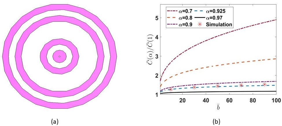
Figure 1: (a) Cross-sectional view of cantor-shaped Mica cylinder (second iteration) with a removal factor of 1/3, which has $\alpha=0.925$ (from box counting method). The pink region is dielectric and the white region is air. (b) The enhancement of the cylindrical capacitance over the $\alpha$ = 1 limit as a function of $\bar{b}$ for different $\alpha$. The asterisks (at $\alpha=0.925$) are the CST simulation results for comparison.

To verify Eq. (29), we create a cylindrical cantor-like (in radial direction) fractal structure with a removal factor of $1/3$ using CST studio suite (see Fig 1(a)). The pink and white regions are dielectric ($\epsilon_{r}=6$) and air space, respectively. Using box-counting method, it has an overall fractional value of $\alpha=(1.776+1)/3=0.925$, where $1.776$ is the fractional value of the 2D cross section of the cylindrical capacitor (Fig. 1a). In Fig 1(b), we plot the ratio of $\bar{C}(\alpha)$ to $\bar{C}(1)$ as a function of $\bar{b}$ = 1 to 100 for various $\alpha$ = 0.7, 0.8, 0.9, 0.925, and 0.97. It shows enhancement as the porosity of a cylinder increases (smaller $\alpha<1$). At $\alpha$ = 0.925, good agreement is observed between the calculated and simulated results.

III.1 Cylindrical MG law for a trap-free solid

In this section, the 1D MG law for a porous cylindrical diode is derived using the fractional capacitance obtained above. When an electron transits the cylindrical gap between anode and cathode, the average normalized electron’s velocity $<\bar{\nu}>$ is calculated by

$$<\bar{\nu}> =\frac{\int_{1}^{\bar{b}}\bar{\nu}(\bar{r})d\bar{r}}{\int_{1}^{\bar{b}}d\bar{r}^{\alpha}}=\dfrac{\alpha\Gamma(\alpha/2)\bar{V}}{\pi^{\alpha/2}(\bar{b}^{\alpha}-1)}$$ (30)

where $\bar{\nu}=\nu/\nu_{0}$ with $\nu_{0}=\mu V_{0}/a$ and the corresponding average transit time is $<\bar{\tau}>=\int_{1}^{\bar{b}}d\bar{r}^{\alpha}/\bar{<\nu>}$. The normalized current line density is defined as $\bar{I}=\frac{I/L}{I_{0}/a}=\dfrac{\bar{Q}}{<\bar{\tau}>}$, and we have

$$\begin{split}\bar{I}&=\frac{2\pi^{1-\frac{3\alpha}{2}}\alpha^{2}s\bar{L}\epsilon_{r}\Gamma\left(\frac{\alpha}{2}\right)^{3}(p+q)\bar{V}^{2}\bar{b}^{-\alpha+\frac{q}{p}+2}}{p\left(\bar{b}^{\alpha}-1\right)^{2}\left(\bar{b}^{\frac{p+q}{p}}-1\right)}=\frac{2\pi^{1-\frac{3\alpha}{2}}\alpha^{3}\bar{b}\bar{L}\epsilon\Gamma\left(\frac{\alpha}{2}\right)^{3}\bar{V}^{2}}{\left(\bar{b}^{\alpha}-1\right)^{3}}\end{split}$$ (31)

where all the constants are $q=\alpha-1$, $p$ = 1 and $s$ = 1 as shown above. The normalized time scale and line current density are $\tau_{0}=\mu V_{0}/a^{2}$ and $I_{0}=Q_{0}\tau_{0}^{-1}$. Considering the current continuity condition, we determine the electric potential as $\bar{V}(\bar{r})=\frac{(\bar{r}^{\alpha}-1)^{3/2}}{(\bar{b}^{\alpha}-1)^{3/2}}$. Using this expression, we can obtain the electron velocity and charge density at the anode $(\bar{r}=\bar{b})$ by solving $\nabla_{\alpha}\bar{V}$ and $\epsilon_{r}\times\nabla^{2}_{\alpha}\bar{V}$ at $\phi=0$ defined in Eq. (27), which are $\bar{\nu}(\bar{r}=\bar{b})=\frac{3}{2}\frac{\alpha\Gamma(\alpha/2)}{\pi^{\alpha/2}(\bar{b}^{\alpha}-1)}$, and $\bar{\rho}(\bar{r}=\bar{b})=\frac{3}{4}\frac{\alpha^{2}\epsilon_{r}\Gamma\left(\frac{\alpha}{2}\right)^{2}}{\pi^{\alpha}\left(\bar{b}^{\alpha}-1\right)^{2}}$. The cylindrical MG law for a porous solid is determined by $\bar{I}(\alpha)=2\pi\bar{b}\bar{\nu}(\bar{r}=\bar{b})\bar{\rho}(\bar{r}=\bar{b})$:

$$\begin{split}\bar{I}(\alpha)&=\frac{9\pi^{1-\frac{3\alpha}{2}}\alpha^{3}\epsilon_{r}\bar{b}\Gamma(\alpha/2)^{3}}{4(\bar{b}^{\alpha}-1)^{3}}.\end{split}$$ (32)

III.2 Cylindrical MH law for a trap-limited solid

To extend the cylindrical model for a trap-filled porous solid, we first, suppose that the injected electrons will fill up the traps bounded given by

$$\bar{Q_{t}} =\bar{\rho_{t}}\int_{0}^{2\pi}d\phi\int_{1}^{\bar{b}}\bar{r}d\bar{r}^{\alpha}=\bar{C}\bar{V}$$ (33)

Using Eq. (18), the line charge density of the free electrons is

$$\bar{Q_{f}} =\int_{0}^{2\pi}d\phi\int_{1}^{\bar{b}}\bar{r}d\bar{r}^{\alpha}\quad\bar{e}\bar{N_{c}}\Big{[}\dfrac{\bar{C}\bar{V}}{\bar{e}\bar{N_{t}}\int_{0}^{2\pi}d\phi\int_{1}^{\bar{b}}\bar{r}d\bar{r}^{\alpha}}\Big{]}^{l}.$$ (34)

Using this $\bar{Q_{f}}$ and Eq. (30), the current line density can be calculated as $\bar{I}=\bar{Q_{f}}\times<\bar{\nu}>/\int_{1}^{\bar{b}}d\bar{r}^{\alpha}$:

$$\begin{split}\bar{I}&=\frac{2^{l+1}\pi^{1-\frac{\alpha}{2}}\alpha^{2}\Gamma\left(\frac{\alpha}{2}\right)\left(\bar{b}^{\alpha+1}-1\right)\bar{V}}{(\alpha+1)\left(\bar{b}^{\alpha}-1\right)^{2}}\left(\frac{\epsilon_{r}\pi^{1-\alpha}\alpha(\alpha+1)\bar{b}\bar{L}\bar{V}\Gamma\left(\frac{\alpha}{2}\right)^{2}}{\left(\bar{b}^{\alpha}-1\right)\left(\bar{b}^{\alpha+1}-1\right)}\right)^{l}.\end{split}$$ (35)

The electrical potential is in the form of

$$\bar{V}(\bar{r}) =\frac{\left(\bar{r}^{\alpha}-1\right)^{\frac{2+l}{l+1}}\left(\bar{r}^{\alpha+1}-1\right)^{\frac{l-1}{l+1}}}{\left(\bar{b}^{\alpha}-1\right)^{\frac{2+l}{l+1}}\left(\bar{b}^{\alpha+1}-1\right)^{\frac{l-1}{l+1}}},$$ (36)

and the MH law for a cylindrical porous solid becomes

$$\bar{I}(\alpha) =2\pi\bar{b}\bar{\nu}(\bar{b})\bar{\rho_{f}}(\bar{b}).$$ (37)

Here, $\bar{\nu}(\bar{b})$ and $\bar{\rho_{f}}(\bar{b})$ is respectively, the electron’s velocity and free electron density at the anode, which are

$$\bar{\nu}(\bar{b}) =\frac{\Gamma\left(\frac{\alpha}{2}\right)\{(\alpha+2\alpha l+l-1)\bar{b}^{\alpha+1}-(\alpha+1)(l-1)\bar{b}-\alpha(l+2)\}}{\pi^{\frac{\alpha}{2}}(l+1)\left(\bar{b}^{\alpha}-1\right)\left(\bar{b}^{\alpha+1}-1\right)},$$ (38)

$$\bar{\rho_{f}}(\bar{b}) =\bar{e}\bar{N_{c}}\left(\frac{\bar{\rho_{t}}(\bar{b})}{\bar{e}\bar{N_{t}}}\right)^{l},$$ (39)

$$\bar{\rho_{t}}(\bar{b}) =\frac{1}{(l+1)^{2}\left(\bar{b}^{\alpha}-1\right)^{2}\left(\bar{b}^{\alpha+1}-1\right)^{2}}\Big{[}\pi^{-\alpha}\Gamma\left(\frac{\alpha}{2}\right)^{2}\epsilon_{r}\bar{b}^{-\alpha}\{(5\alpha-\left(2\alpha^{2}+3\alpha+1\right)l^{2}-$$

$$\quad{}2\alpha(2\alpha+1)l+1)\bar{b}^{2\alpha+1}+\left(-\alpha+\left(2\alpha^{2}+3\alpha+1\right)l^{2}+\left(\alpha^{2}-2\alpha-2\right)l+1\right)\bar{b}^{3\alpha+2}-$$

$$\quad{}(\alpha+1)\left(l^{2}-1\right)\bar{b}+\alpha^{2}(l+2)\bar{b}^{\alpha}+2(\alpha+1)(l-1)(2\alpha+\alpha l+l+1)\bar{b}^{\alpha+1}+$$

$$\quad{}(\alpha+1)(l-1)(-2\alpha+l-1)\bar{b}^{\alpha+2}-2(\alpha+1)(l-1)(\alpha l+l-1)\bar{b}^{2\alpha+2}\}\Big{]}.$$ (40)

In Fig. 2, we show the the enhancement of the MH law: $\bar{I}(\alpha)$ over its limit at $\alpha=1$ (classical MH law) as a function of $\bar{b}$ = 1 to 100 for $\alpha=$0.7, 0.8, 0.9 and 0.97. Four cases of different traps ($l=$1, 3, 5 and 7) are presented to see the effect of trap-limited current. At $l=$1, we recover the trap-free case (or MG law) as shown in Eq. (32).

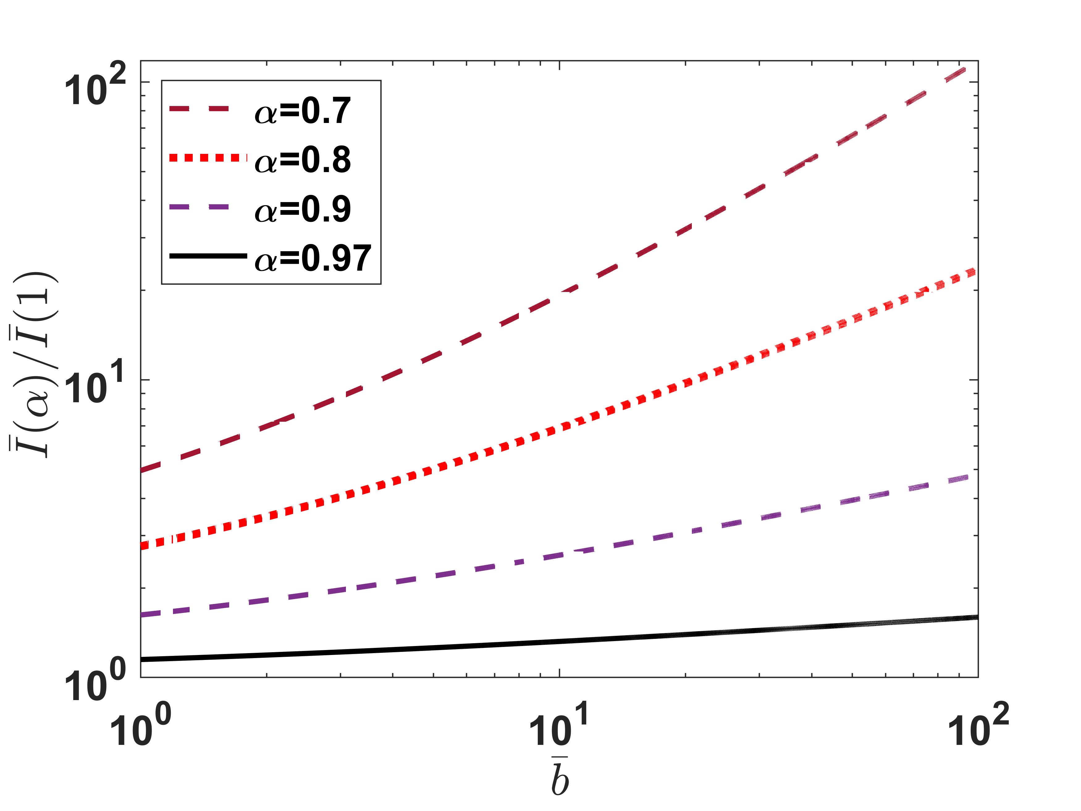
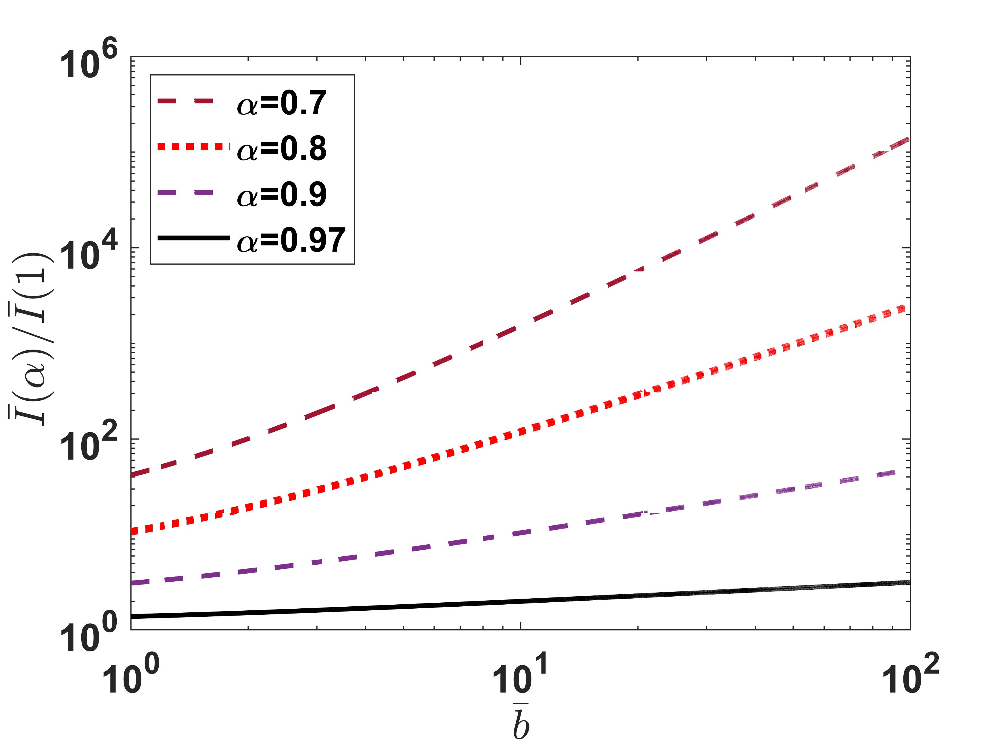
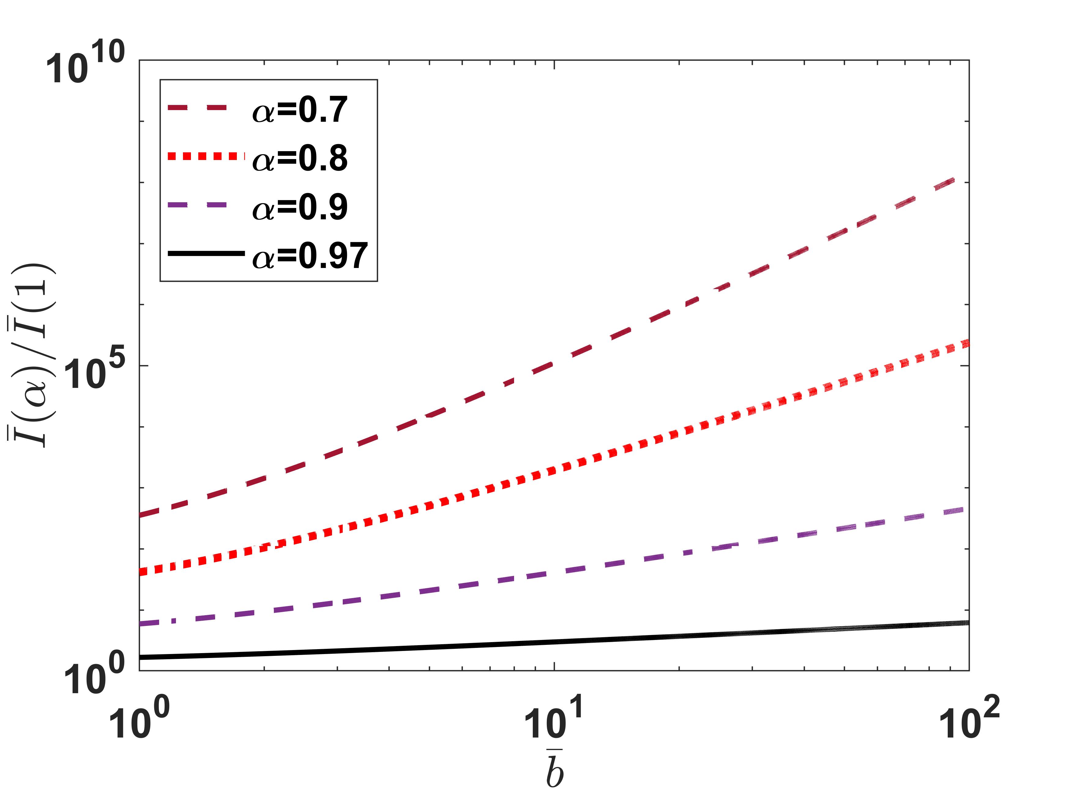
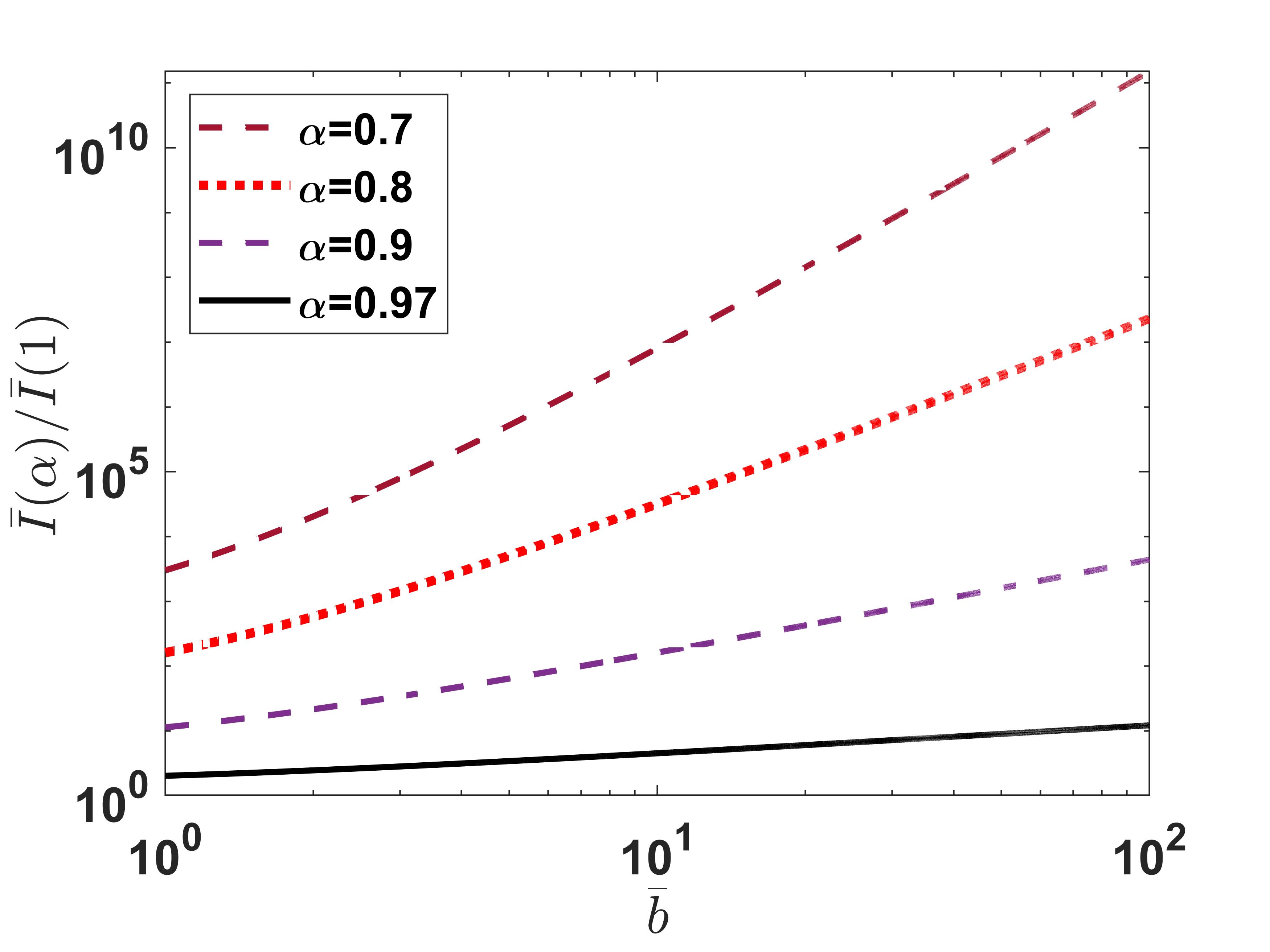
Figure 2: Enhancement of the cylindrical MH law with $\alpha<$ 1 over the limit at $\alpha$ = 1 as a function of $\bar{b}$ for (a) $l$=1 [MG law], (b) $l$=3, (c) $l$=5, and (d) $l$=7.

Due to the absence of MH law for cylindrical diode without porosity effects (perfect solid), we compare our fractional cylindrical MH law at $\alpha=1$ and $l=1$ (or MG law) with a prior result Meltzer (1960) in Fig. 3(a), which shows good agreements over a wide range of $\bar{b}$ = 1 to 100. For cylindrical diode with large aspect ratio of $\bar{b}=b/a\rightarrow\infty$, our analytical results also agree with a prior analytical formulation Zhu and Ang (2011b) at $\bar{b}\geq$ 10. It is important to note that our newly derived analytical formulation of cylindrical MH law for a porous solid [Eqs. (37) to (40)] is applicable for any $l$, $\alpha$, and $\bar{b}$.

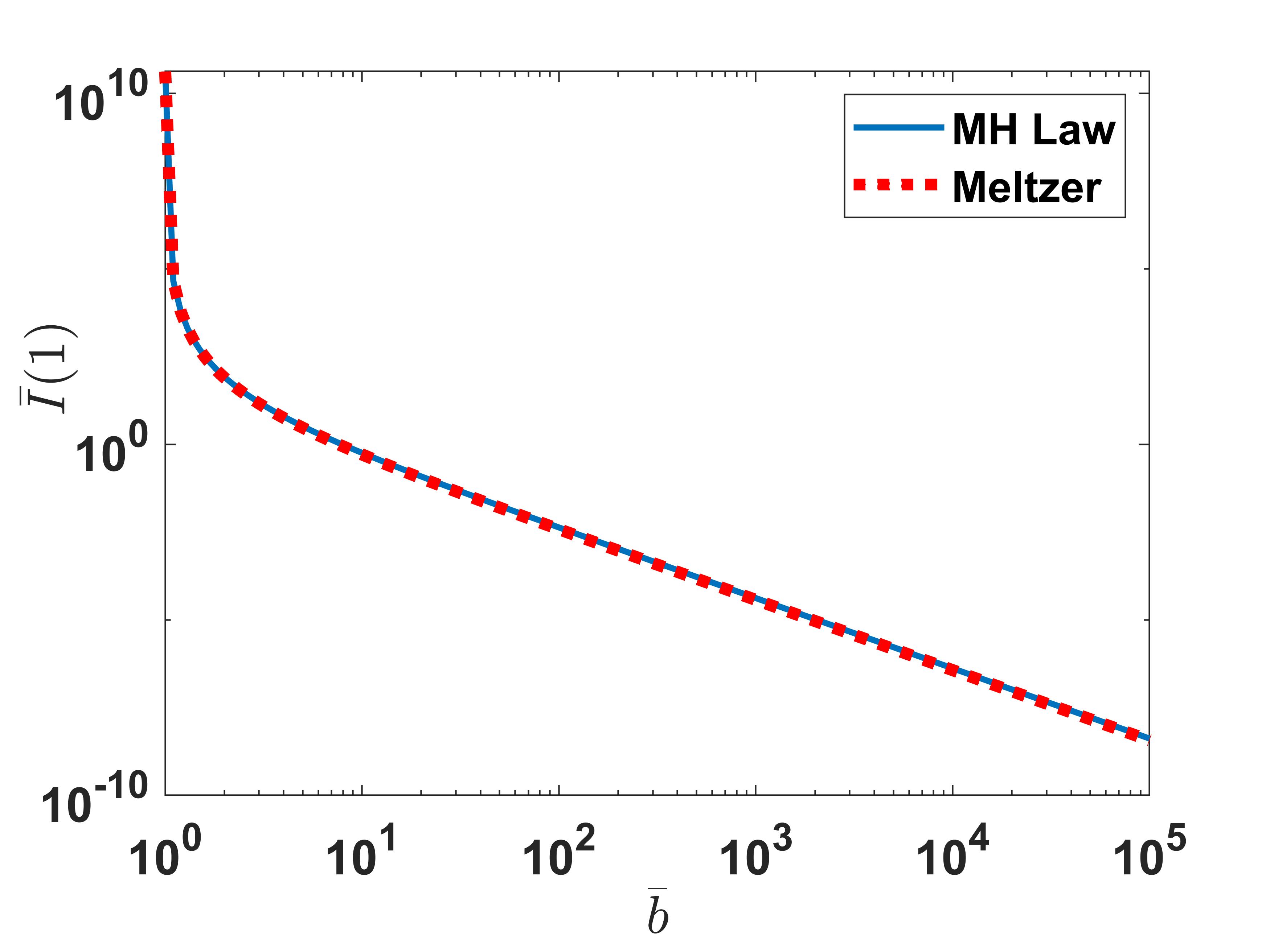
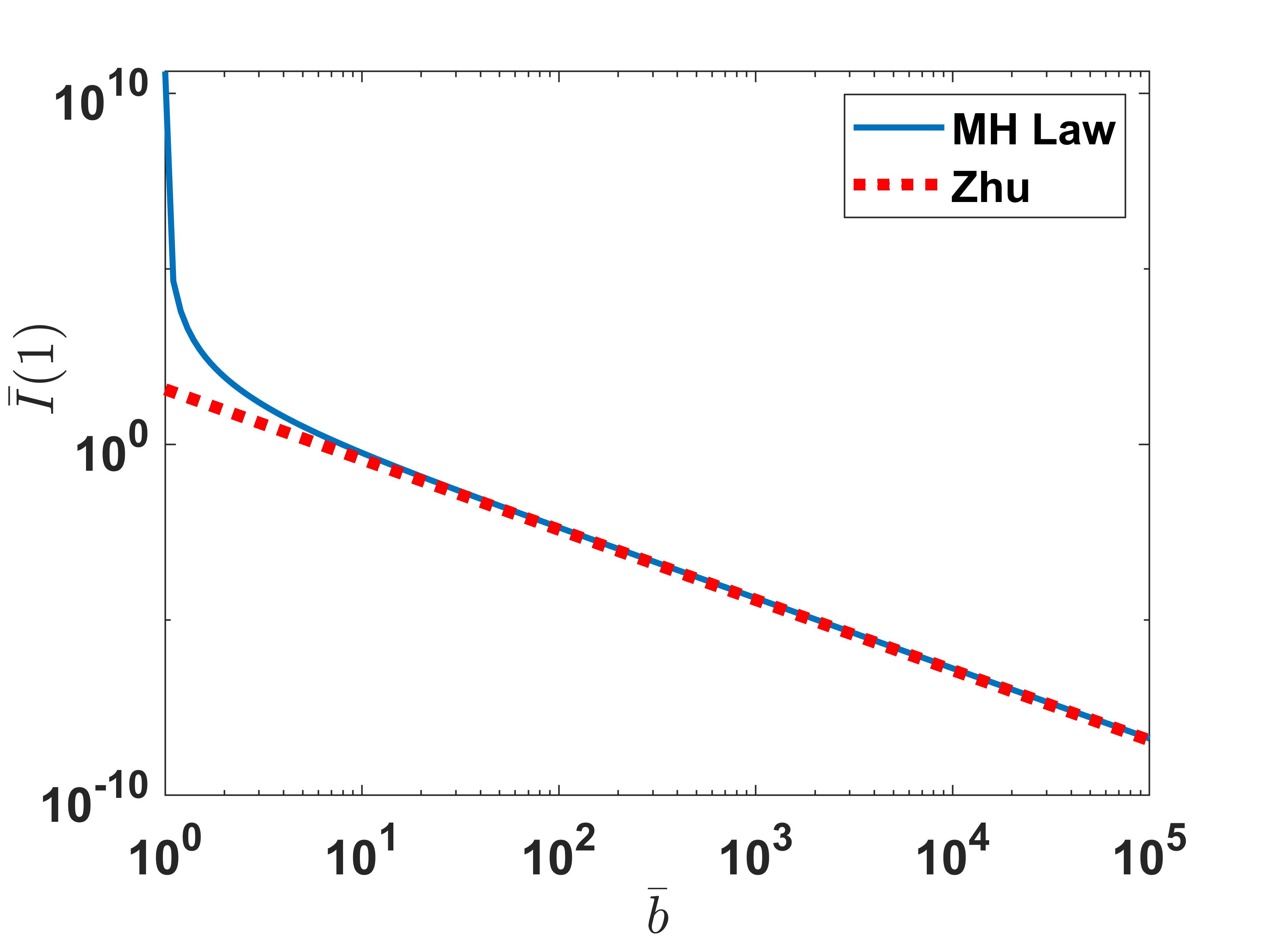
Figure 3: Comparison of the derived analytical MH law at $\alpha=1$ and $l=1$ from Eq. (37) with two prior works: (a) by Meltzer Meltzer (1960) and (b) by Zhu Zhu and Ang (2011b) at $\bar{b}\rightarrow\infty$.

IV Conclusion

In this work, we have presented a cylindrical space charge limited current (SCLC) model or MH law for a porous trap-limited dielectric characterized by $\alpha\leq$ 1. The analytical model is derived for the first time by using different formulations involving capacitance and transit time models. The results are verified in recovering the planar case and at $\alpha$ = 1 limit (perfect solid without porosity), such as Mott-Gurney (MG) law and Mark-Helfrich (MH) law for trap-free and trap-limited case respectively. In the applications of SCLC transport in organic electronics and dielectric breakdown, where the spatial porosity of the material is ubiquitous, this novel model can be a valuable tool for characterizing the porosity by fitting our analytical model to the current-voltage measurements.

AUTHOR DECLARATIONS

Conflict of Interest

The authors have no conflicts to disclose.

Data Availability

The data that support the findings of this study are available from the corresponding author upon reasonable request.

References

- Child (1911) C. D. Child, “Discharge from hot CaO,” Phys. Rev. (Series I) 32, 492 (1911).
- Langmuir (1913) I. Langmuir, “The effect of space charge and residual gases on thermionic currents in high vacuum,” Phys. Rev. 2, 450 (1913).
- Lau et al. (1991) Y. Y. Lau, D. Chernin, D. G. Colombant, and P.-T. Ho, “Quantum extension of Child-Langmuir law,” Phys. Rev. Lett. 66, 1446 (1991).
- Ang, Kwan, and Lau (2003) L. K. Ang, T. J. T. Kwan, and Y. Y. Lau, “New scaling of Child-Langmuir law in the quantum regime,” Phys. Rev. Lett. 91, 208303 (2003).
- Ang, Lau, and Kwan (2004) L. K. Ang, Y. Y. Lau, and T. J. T. Kwan, “Simple derivation of quantum scaling in Child-Langmuir law,” IEEE Trans. Plasma Sci. 32, 410–412 (2004).
- Bhattacharjee, Vartak, and Mukherjee (2008) S. Bhattacharjee, A. Vartak, and V. Mukherjee, “Experimental study of space-charge-limited flows in a nanogap,” Appl. Phys. Lett. 92, 191503 (2008).
- Luginsland, Lau, and Gilgenbach (1996) J. Luginsland, Y. Y. Lau, and R. Gilgenbach, “Two-dimensional Child-Langmuir law,” Phys. Rev. Lett. 77, 4668 (1996).
- Lau (2001) Y. Y. Lau, “Simple theory for the two-dimensional Child-Langmuir law,” Phys. Rev. Lett. 87, 278301 (2001).
- Koh, Ang, and Kwan (2005) W. Koh, L. K. Ang, and T. J. T. Kwan, “Three-dimensional Child-Langmuir law for uniform hot electron emission,” Phys. Plasmas 12, 053107 (2005).
- Umstattd and Luginsland (2001) R. J. Umstattd and J. W. Luginsland, “Two-dimensional space-charge-limited emission: Beam-edge characteristics and applications,” Phys. Rev. Lett. 87, 145002 (2001).
- Sree Harsha et al. (2021) N. R. Sree Harsha, M. Pearlman, J. Browning, and A. L. Garner, “A multi-dimensional Child–Langmuir law for any diode geometry,” Phys. Plasmas 28, 122103 (2021).
- Valfells et al. (2002) Á. Valfells, D. Feldman, M. Virgo, P. O’shea, and Y. Y. Lau, “Effects of pulse-length and emitter area on virtual cathode formation in electron guns,” Phys. Plasmas 9, 2377–2382 (2002).
- Ang and Zhang (2007) L. K. Ang and P. Zhang, “Ultrashort-pulse Child-Langmuir law in the quantum and relativistic regimes,” Phys. Rev. Lett. 98, 164802 (2007).
- Pedersen, Manolescu, and Valfells (2010) A. Pedersen, A. Manolescu, and Á. Valfells, “Space-charge modulation in vacuum microdiodes at THz frequencies,” Phys. Rev. Lett. 104, 175002 (2010).
- Zhu and Ang (2011a) Y. Zhu and L. K. Ang, “Child–Langmuir law in the coulomb blockade regime,” Appl. Phys. Lett. 98, 051502 (2011a).
- Chen et al. (2011) S. Chen, L. Tai, Y. Liu, L. K. Ang, and W. Koh, “Two-dimensional electromagnetic Child–Langmuir law of a short-pulse electron flow,” Phys. Plasmas 18, 023105 (2011).
- Zubair and Ang (2016) M. Zubair and L. K. Ang, “Fractional-dimensional Child-Langmuir law for a rough cathode,” Phys. Plasmas 23, 072118 (2016).
- Zhu and Ang (2015) Y. B. Zhu and L. K. Ang, “Space charge limited current emission for a sharp tip,” Phys. Plasmas 22, 052106 (2015).
- Chernin et al. (2020) D. Chernin, Y. Y. Lau, J. J. Petillo, S. Ovtchinnikov, D. Chen, A. Jassem, R. Jacobs, D. Morgan, and J. H. Booske, “Effect of nonuniform emission on miram curves,” IEEE Trans. Plasma Sci. 48, 146–155 (2020).
- Jassem et al. (2021) A. Jassem, D. Chernin, J. J. Petillo, Y. Y. Lau, A. Jensen, and S. Ovtchinnikov, “Analysis of anode current from a thermionic cathode with a 2-D work function distribution,” IEEE Trans. Plasma Sci. 49, 749–755 (2021).
- Sitek et al. (2021a) A. Sitek, K. Torfason, A. Manolescu, and Á. Valfells, “Space-charge effects in the field-assisted thermionic emission from nonuniform cathodes,” Phys. Rev. Appl. 15, 014040 (2021a).
- Chen et al. (2022) D. Chen, R. Jacobs, J. Petillo, V. Vlahos, K. L. Jensen, D. Morgan, and J. Booske, “Physics-based model for nonuniform thermionic electron emission from polycrystalline cathodes,” Phys. Rev. Appl. 18, 054010 (2022).
- Sitek et al. (2021b) A. Sitek, K. Torfason, A. Manolescu, and Á. Valfells, “Edge effect on the current-temperature characteristic of finite-area thermionic cathodes,” Phys. Rev. Appl. 16, 034043 (2021b).
- Zhang et al. (2017) P. Zhang, Á. Valfells, L. K. Ang, J. W. Luginsland, and Y. Y. Lau, “100 years of the physics of diodes,” Appl. Phys. Rev. 4, 011304 (2017).
- Zhang et al. (2021) P. Zhang, Y. S. Ang, A. L. Garner, Á. Valfells, J. W. Luginsland, and L. K. Ang, “Space-charge limited current in nanodiodes: Ballistic, collisional, and dynamical effects,” J. Appl. Phys. 129, 100902 (2021).
- Lampert and Mark (1970) M. A. Lampert and P. Mark, Current injection in solids (Academic press, 1970).
- Mark and Helfrich (1962) P. Mark and W. Helfrich, “Space-charge-limited currents in organic crystals,” J. Appl. Phys. 33, 205–215 (1962).
- Chandra et al. (2007) W. Chandra, L. K. Ang, K. L. Pey, and C. M. Ng, “Two-dimensional analytical Mott-Gurney law for a trap-filled solid,” Appl. Phys. Lett. 90, 153505 (2007).
- Kee et al. (2022a) C. Y. Kee, Y. S. Ang, E.-P. Li, and L. K. Ang, “Analytical scaling of trap-limited current in 2-D ultrathin dielectrics,” IEEE Trans. Electron Devices (2022a).
- Chandra, Ang, and Koh (2009) W. Chandra, L. K. Ang, and W. S. Koh, “Two-dimensional model of space charge limited electron injection into a diode with schottky contact,” J. Phys. D: Appl. Phys. 42, 055504 (2009).
- Paasch and Scheinert (2009) G. Paasch and S. Scheinert, “Space-charge-limited currents in organics with trap distributions: Analytical approximations versus numerical simulation,” J. Appl. Phys. 106, 084502 (2009).
- Zhang and Pantelides (2012) X.-G. Zhang and S. T. Pantelides, “Theory of space charge limited currents,” Phys. Rev. Lett. 108, 266602 (2012).
- López Varo et al. (2012) P. López Varo, J. Jiménez Tejada, J. López Villanueva, J. Carceller, and M. Deen, “Modeling the transition from ohmic to space charge limited current in organic semiconductors,” Org. Electron. 13, 1700–1709 (2012).
- López Varo et al. (2014) P. López Varo, J. Jiménez Tejada, J. López Villanueva, and M. Deen, “Space-charge and injection limited current in organic diodes: A unified model,” Org. Electron. 15, 2526–2535 (2014).
- Zhu et al. (2021) Y. B. Zhu, K. Geng, Z. S. Cheng, and R. H. Yao, “Space-charge-limited current injection into free space and trap-filled solid,” IEEE Trans. Plasma Sci. 49, 2107–2112 (2021).
- González (2015) G. González, “Quantum theory of space charge limited current in solids,” J. Appl. Phys. 117, 084306 (2015).
- Greenwood et al. (2016) A. Greenwood, J. Hammond, P. Zhang, and Y. Lau, “On relativistic space charge limited current in planar, cylindrical, and spherical diodes,” Phys. Plasmas 23, 072101 (2016).
- Ang, Zubair, and Ang (2017) Y. S. Ang, M. Zubair, and L. K. Ang, “Relativistic space-charge-limited current for massive dirac fermions,” Phys. Rev. B 95, 165409 (2017).
- Stöckmann (2022) F. Stöckmann, “An exact evaluation of steady-state space-charge-limited currents for arbitrary trap distributions,” in Volume 64, Number 2 April 16 (De Gruyter, 2022) pp. 475–484.
- Röhr et al. (2018) J. A. Röhr, X. Shi, S. A. Haque, T. Kirchartz, and J. Nelson, “Charge transport in spiro-ometad investigated through space-charge-limited current measurements,” Phys. Rev. Appl. 9, 044017 (2018).
- Fratini et al. (2020) S. Fratini, M. Nikolka, A. Salleo, G. Schweicher, and H. Sirringhaus, “Charge transport in high-mobility conjugated polymers and molecular semiconductors,” Nat. Mater. 19, 491–502 (2020).
- Akgül et al. (2021) F. D. Akgül, S. Eymur, Ü. Akın, Ö. F. Yüksel, H. Karadeniz, and N. Tuğluoğlu, “Investigation of Schottky emission and space charge limited current (SCLC) in Au/SnO2/n-Si Schottky diode with gamma-ray irradiation,” J. Mater. Sci.: Mater. Electron. 32, 15857–15863 (2021).
- Vermeersch et al. (2022) R. Vermeersch, G. Jacopin, B. Daudin, and J. Pernot, “DX center formation in highly Si doped AlN nanowires revealed by trap assisted space-charge limited current,” Appl. Phys. Lett. 120, 162104 (2022).
- Torricelli, Zappa, and Colalongo (2010) F. Torricelli, D. Zappa, and L. Colalongo, “Space-charge-limited current in organic light emitting diodes,” Appl. Phys. Lett. 96, 51 (2010).
- Park, Kim, and Cho (2018) J. H. Park, J. K. Kim, and J. Cho, “Observation of space-charge-limited current in AlGaN/GaN ultraviolet light-emitting diodes,” Mater. Lett. 214, 217–219 (2018).
- Carbone, Kotowska, and Kotowski (2005) A. Carbone, B. Kotowska, and D. Kotowski, “Space-charge-limited current fluctuations in organic semiconductors,” Phys. Rev. letters 95, 236601 (2005).
- Carbone, Pennetta, and Reggiani (2009) A. Carbone, C. Pennetta, and L. Reggiani, “Trapping-detrapping fluctuations in organic space-charge layers,” Appl. Phys. Lett. 95, 318 (2009).
- Craciun, Wildeman, and Blom (2008) N. Craciun, J. Wildeman, and P. Blom, “Universal arrhenius temperature activated charge transport in diodes from disordered organic semiconductors,” Phys. Rev. Lett. 100, 056601 (2008).
- Matsushima and Murata (2009) T. Matsushima and H. Murata, “Observation of space-charge-limited current due to charge generation at interface of molybdenum dioxide and organic layer,” Appl. Phys. Lett. 95, 301 (2009).
- Rojek, Schmechel, and Benson (2019) K. Rojek, R. Schmechel, and N. Benson, “Ultra-fast measurement circuit for transient space charge limited current in organic semiconductor thin films,” Meas. Sci. Technol. 31, 015901 (2019).
- Tsormpatzoglou et al. (2006) A. Tsormpatzoglou, D. Tassis, C. Dimitriadis, L. Dózsa, N. Galkin, D. Goroshko, V. Polyarnyi, and E. Chusovitin, “Deep levels in silicon Schottky junctions with embedded arrays of -FeSi2 nanocrystallites,” J. Appl. Phys. 100, 074313 (2006).
- Zubair, Ang, and Ang (2018a) M. Zubair, Y. S. Ang, and L. K. Ang, “Thickness dependence of space-charge-limited current in spatially disordered organic semiconductors,” IEEE Trans. Electron Devices 65, 3421–3429 (2018a).
- Zhu et al. (2013) Y. B. Zhu, P. Zhang, Á. Valfells, L. K. Ang, and Y. Y. Lau, “Novel scaling laws for the Langmuir-Blodgett solutions in cylindrical and spherical diodes,” Phys. Rev. Lett. 110, 265007 (2013).
- Darr and Garner (2019) A. M. Darr and A. L. Garner, “A coordinate system invariant formulation for space-charge limited current in vacuum,” Appl. Phys. Lett. 115, 054101 (2019).
- Song et al. (2021) M. Song, Q. Zhou, H. Zhang, W. Yang, Q. Sun, and Y. Dong, “Comment on “a coordinate system invariant formulation for space-charge limited current in vacuum” [Appl. Phys. Lett. 115, 054101 (2019)],” Appl. Phys. Lett. 119, 206101 (2021).
- Darr, Sree Harsha, and Garner (2021) A. M. Darr, N. R. Sree Harsha, and A. L. Garner, “Response to “comment on ‘a coordinate system invariant formulation for space-charge limited current in vacuum’” [Appl. Phys. Lett. 119, 206101 (2021)],” Appl. Phys. Lett. 119, 206102 (2021).
- Garner, Darr, and Harsha (2022) A. L. Garner, A. M. Darr, and N. R. S. Harsha, “A tutorial on calculating space-charge-limited current density for general geometries and multiple dimensions,” IEEE Trans. Plasma Sci. 50, 2528–2540 (2022).
- Zhu and Ang (2011b) Y. Zhu and L. K. Ang, “Analytical re-derivation of space charge limited current in solids using capacitor model,” J. Appl. Phys. 110, 094514 (2011b).
- Kanwal et al. (2022) S. Kanwal, C. Y. Kee, S. Y. Low, M. Zubair, and L. K. Ang, “Capacitance for fractal-like disordered dielectric slab,” J. Appl. Phys. 132, 024104 (2022).
- Tarasov (2008) V. E. Tarasov, “Fractional vector calculus and fractional Maxwell’s equations,” Ann. Phys. 323, 2756–2778 (2008).
- Tarasov (2019) V. E. Tarasov, ed., Applications in Physics, Part B (De Gruyter, Berlin, Boston, 2019).
- Tarasov (2005) V. E. Tarasov, “Fractional hydrodynamic equations for fractal media,” Ann. Phys. 318, 286–307 (2005).
- Balankin and Elizarraraz (2012) A. S. Balankin and B. E. Elizarraraz, “Map of fluid flow in fractal porous medium into fractal continuum flow,” Phys. Rev. E 85, 056314 (2012).
- Tarasov (2016) V. E. Tarasov, “Heat transfer in fractal materials,” Int. J. Heat Mass Transfer 93, 427–430 (2016).
- Zubair, Mughal, and Naqvi (2012) M. Zubair, M. J. Mughal, and Q. A. Naqvi, “Differential electromagnetic equations in fractional space,” in Electromagnetic Fields and Waves in Fractional Dimensional Space (Springer, 2012) pp. 7–16.
- Bukhari et al. (2022) A. H. Bukhari, M. A. Z. Raja, N. Rafiq, M. Shoaib, A. K. Kiani, and C.-M. Shu, “Design of intelligent computing networks for nonlinear chaotic fractional Rossler system,” Chaos, Solitons & Fractals 157, 111985 (2022).
- Xu et al. (2021) X.-Y. Xu, X.-W. Wang, D.-Y. Chen, C. M. Smith, and X.-M. Jin, “Quantum transport in fractal networks,” Nat. Photonics 15, 703–710 (2021).
- Kotimäki et al. (2013) V. Kotimäki, E. Räsänen, H. Hennig, and E. J. Heller, “Fractal dynamics in chaotic quantum transport,” Phys. Rev. E 88, 022913 (2013).
- Ahmad et al. (2020) S. Ahmad, M. Zubair, O. Jalil, M. Q. Mehmood, U. Younis, X. Liu, K. W. Ang, and L. K. Ang, “Generalized scaling law for exciton binding energy in two-dimensional materials,” Phys. Rev. Appl. 13, 064062 (2020).
- Zubair, Ang, and Ang (2018b) M. Zubair, Y. S. Ang, and L. K. Ang, “Fractional Fowler–Nordheim law for field emission from rough surface with nonparabolic energy dispersion,” IEEE Trans. Electron Devices 65, 2089–2095 (2018b).
- Zubair et al. (2018) M. Zubair, Y. S. Ang, K. J. A. Ooi, and L. K. Ang, “Fractional Fresnel coefficients for optical absorption in femtosecond laser-induced rough metal surfaces,” J. Appl. Phys. 124, 163101 (2018).
- Kee et al. (2022b) C. Y. Kee, C. Chua, M. Zubair, and L. K. Ang, “Fractional modeling of urban growth with memory effects,” Chaos 32, 083127 (2022b).
- Safdari et al. (2016) H. Safdari, M. Z. Kamali, A. Shirazi, M. Khalighi, G. Jafari, and M. Ausloos, “Fractional dynamics of network growth constrained by aging node interactions,” PLOS ONE 11, e0154983 (2016).
- Sun et al. (2018) H. Sun, Y. Zhang, D. Baleanu, W. Chen, and Y. Chen, “A new collection of real world applications of fractional calculus in science and engineering,” Commun. Nonlinear Sci. Numer. Simul. 64, 213–231 (2018).
- Mott and Gurney (1948) N. F. Mott and R. W. Gurney, Electronic processes in ionic crystals (Clarendon Press, 1948).
- Meltzer (1960) B. Meltzer, “Space-charge-limited currents in cylindrical and spherical insulator diodes,” Int. J. Electron. 8, 171–176 (1960).
- Zubair et al. (2023) M. Zubair, A. Fatima, N. Raheem, Y. S. Ang, M. Q. Mehmood, and Y. Massoud, “Coordinate system invariant formulation of fractional-dimensional Child-Langmuir law for a rough cathode,” Adv. Phys. Res. (2023).