Online Interior-point Methods for Time-varying Equality-constrained Optimization

Abstract

An important challenge in the online convex optimization (OCO) setting is to incorporate generalized inequalities and time-varying constraints. The inclusion of constraints in OCO widens the applicability of such algorithms to dynamic but safety-critical settings such as the online optimal power flow (OPF) problem. In this work, we propose the first projection-free OCO algorithm admitting time-varying linear constraints and convex generalized inequalities: the online interior-point method for time-varying equality constraints (OIPM-TEC). We derive simultaneous sublinear dynamic regret and constraint violation bounds for OIPM-TEC under standard assumptions. For applications where a given tolerance around optima is accepted, we propose a new OCO performance metric – the epsilon-regret – and a more computationally efficient algorithm, the epsilon OIPM-TEC, that possesses sublinear bounds under this metric. Finally, we showcase the performance of these two algorithms on an online OPF problem and compare them to another OCO algorithm from the literature.

Online convex optimization, Optimization algorithms, Time-varying systems, Machine learning

1 Introduction

Online convex optimization (OCO) with time-varying constraints, henceforth referred to as constrained OCO, is an emerging field with many practical applications including network resource allocation [1], portfolio selection [2], and control of electric grids [3] or of multi-energy systems [4]. In OCO, an agent makes sequential decisions to minimize an environment-determined loss function [2, 5, 6]. Constrained OCO adds the requirement that the decision sequence is subject to time-varying constraints. Integrating online or time-varying constraints is essential to ensure effective implementation of OCO algorithms in safety-critical applications. The performance of a constrained OCO algorithm is measured both in terms of its regret and its constraint violation [7, 5]. These represent the cumulative distance from optimality and from feasibility, respectively. Regret can be calculated either by comparing the decision sequence to the best fixed decision in hindsight (static regret) or to the round-optimal decision (dynamic regret) [8]. The dynamic regret is a tighter metric than the static regret as a bounded dynamic regret guarantees a bounded static regret [9]. When designing an OCO algorithm, the objective is to obtain sublinear regret and constraint violation bounds which imply the time-averaged regret and constraint violation will go to zero as the time-horizon goes to infinity [2, 5, 9]. This means implemented decisions will be optimal and feasible, on average, over a long time horizon.

A promising application of constrained OCO is the online optimal power flow (OPF) problem. The OPF problem consists of finding the optimal power generation profile that minimizes costs for the operator of the electric grid while ensuring that all loads are adequately supplied and that physical and safety limits are respected [10]. This problem is non-convex and thus NP-hard to solve. For this reason, multiple convex relaxations of the OPF have been formulated to compute an approximated solution in polynomial time [10, 11, 12]. However, the tightest relaxations are conic relaxations that leverage generalized inequalities [12]. This makes solving these problems tedious and time-consuming in large-scale systems. In modern power grids, the integration of renewable energy sources introduce power fluctuations on a significantly faster timescale when compared to conventional generators [13]. This makes the traditional approach of solving the OPF every 15-30 minutes [3, 14] unable to conform to the renewable timescale. The efficiency, adaptability, and resiliency of constrained OCO algorithms can overcome this limitation.

However, solving a conic relaxation of the OPF problem in an OCO context is challenging for multiple reasons. First and foremost is the integration of time-varying equality constraints linked to changes in power demand. Addressing the generalized inequalities associated with the conic constraints is also an obstacle. Many OCO algorithms use a projection step [9, 15, 16] onto the feasible space defined by these constraints. This is problematic because when the feasible space is the cone of positive semi-definite (PSD) matrices or a second-order cone – as is the case in the relaxed OPF – the projection can be as costly as solving the offline problem. Additionally, the less stringent static regret is ill-adapted to an online OPF setting. A fixed solution satisfying the constraints at all timesteps may incur arbitrarily large losses or might not exist at all [9]. Therefore, a candidate OCO algorithm for the online OPF is one admitting time-varying equality constraints, being projection-free, and possessing a sublinear dynamic regret and constraint violation. We propose an online optimization approach based on a primal interior-point method that possesses these three qualities.

Related work

Although many constrained OCO approaches can be found in the literature, none possesses all three required properties necessary to effectively solve the online OPF. The majority of OCO algorithms that admit time-varying constraints use static regret as a performance metric. This metric uses the best fixed decision in hindsight as the comparator sequence. A common approach in this setting is to use a virtual queue to ensure a bounded static regret while satisfying long-term or slowly varying constraints. This approach is equivalent to solving a modified Lagrangian system. Virtual queues are used in [17, 18, 19, 20] to achieve sublinear static regret and constraint violation bounds. The model-based augmented Lagrangian method (MALM) presented in [15] which possesses sublinear regret and constraint violation bounds has been shown to experimentally outperform many of these previous methods. A projection-free OCO algorithm utilising barrier functions as regularizers is presented in [21] which achieves sublinear static regret. This approach does not admit time-varying equality constraints or a dynamic regret bound.

Algorithms with dynamic regret bounds have also been developed to handle time-varying constraints. An online saddle-point method (MOSP) proposed in [9] and an approach using virtual queues presented in [16] possess sublinear dynamic regret and constraint violation bounds. These bounds are, however, predicated on strict limits on objective and constraint function variations as well as time-varying stepsizes. Both these algorithms rely on a costly projection step for conic constraints. Sublinear dynamic regret and constraint violation is obtained in [7] even for non-convex functions. The bounds are looser than those of [9, 16] and the algorithm requires a projection at every iteration. A primal-dual mirror descent approach was proposed in [22] for distributed OCO and analyzed using dynamic regret but the authors only obtained constraint violation bounds that grow linearly with time. A second-order method was presented in [23] for unconstrained optimization which was extended in [24] to admit time-varying equality constraints. Both these approaches have tight dynamic regret bounds but are incompatible with inequality constraints.

Approaches to iteratively solve the OPF have also been presented. An algorithm based on a quasi-Newton update was used to solve the OPF in real-time in [25]. Although this algorithm has good tracking performance under strict conditions, the authors did not derive a bound on constraint violation. A distributed feedback controller is designed in [26] but uses a linear approximation of the OPF rather than a conic relaxation. A model-free online feedback optimization algorithm is presented in [27]. This approach is shown to converge to optimal solutions of the OPF problem but does not have theoretical guarantees on tracking or constraint violation.

In this paper, we present the first constrained OCO algorithm capable of satisfying all three necessary conditions for effective resolution of the online OPF. This is achieved by extending the OPEN-M algorithm from [24] to integrate generalized inequalities using an interior-point method-like update. Our contributions can be summarized as follows:

• We present the first projection-free OCO algorithm that admits convex generalized inequalities and time-varying linear equality constraints while achieving tight sublinear dynamic regret and constraint violation bounds.

• We introduce the notion of epsilon-regret in which one accepts being in an epsilon-neighbourhood of the optimal solution and propose an efficient algorithm possessing tight epsilon-regret and constraint violation bounds.

• We illustrate the performance of our approaches by solving an online OPF based on the 33-bus Matpower case.

2 Preliminaries

In this section, we define useful terms, lay down important assumptions, and introduce the Newton’s step which will be used in the analysis of our main results.

2.1 Definitions

In this work, our goal is to solve time-varying equality constrained OCO problems subject to generalized inequality constraints described in (1). The generalized inequality constraints can, for example, be defined with respect to the cone of positive semidefinite matrices or a second-order cone. Formally, let $\mathbf{c}\in\mathbb{R}^{N}$ be our objective vector with $N\in\mathbb{N}$ the dimension of the decision variable. Let $\mathbf{x}_{t}\in\mathbb{R}^{N}$ be the decision vector at any time $t=0,1,2,...,T$ where $T\in\mathbb{N}$ is the time horizon. All functions $g_{i}(\mathbf{x}):\mathbb{R}^{N}\mapsto\mathbb{R}^{K_{i}}$, $i=1,2,...,I$, $I\in\mathbb{N}$, $K_{i}\in\mathbb{N}$ are assumed to be convex and self-concordant. Self-concordancy is defined in (4) and is a common assumption in the interior-point literature [28, 29]. Let the matrix $\mathbf{A}\in\mathbb{R}^{P\times N}$ be a full row-rank matrix with $P\in\mathbb{N}$, $P<N$. Let the vector $\mathbf{b}_{t}\in\mathbb{R}^{P}$ be time-varying. In the sequel, the norm $\left\lVert\cdot\right\rVert$ denotes the Euclidean norm. In summary, we tackle the following online optimization problem:

$$\begin{split}\min_{\mathbf{x}_{t}}&\quad\mathbf{c}^{\top}\mathbf{x}_{t}\\ \text{s.t.}\quad&g_{i}(\mathbf{x}_{t})\preceq 0,\quad\text{for }i=1,2,3,...,I\\ &\mathbf{A}\mathbf{x}_{t}-\mathbf{b}_{t}=0.\end{split}$$ (1)

We define the optimal decision, $\mathbf{x}_{t}^{*}$, at every timestep as:

$$\mathbf{x}_{t}^{*}\in\operatorname*{arg\,min}_{\mathbf{x}} \quad\mathbf{c}^{\top}\mathbf{x}$$

$$\text{s.t.}\quad g_{i} (\mathbf{x})\preceq 0,\quad\text{for }i=1,2,3,...,I$$

$$\mathbf{A}\mathbf{x}-\mathbf{b}_{t}=0.$$

To measure the performance of constrained OCO algorithms, two metrics are employed: regret and constraint violation. These represent the cumulative distance from optimality and from feasibility, respectively. In this work, dynamic regret is used which uses the round-optimal solution $\mathbf{x}_{t}^{*}$ as a comparator. This can be formally defined as:

$$R_{\text{d}}(T)=\sum_{t=1}^{T}\mathbf{c}^{\top}\mathbf{x}_{t}-\mathbf{c}^{\top}\mathbf{x}_{t}^{*}.$$ (2)

The constraint violation is null if every decision is feasible and positive otherwise. It is defined as:

$$\text{Vio}(T)=\sum_{t=1}^{T}\left[\sum_{i}\left[\text{Tr}\Big{(}g_{i}(\mathbf{x}_{t})\Big{)}\right]^{+}+\left\lVert\mathbf{A}\mathbf{x}_{t}-\mathbf{b}_{t}\right\rVert\right],$$ (3)

where $[x]^{+}$ denotes the $\max\{x,0\}$ operator and Tr denotes the trace operator. We define the cumulative variation between optimal decisions $V_{T}$ as:

$$V_{T}=\sum_{t=1}^{T}\left\lVert\mathbf{x}_{t}^{*}-\mathbf{x}_{t-1}^{*}\right\rVert.$$

Similarly, we define the cumulative variation in the right-hand term of the time-varying equality constraint $\mathbf{b}$ as:

$$V_{\mathbf{b}}=\sum_{t=1}^{T}\left\lVert\mathbf{b}_{t}-\mathbf{b}_{t-1}\right\rVert.$$

Let $\left\lVert\cdot\right\rVert_{\mathbf{x}}$ denote the Hessian norm as in [29]. For any vector $\mathbf{z}\in\mathbb{R}^{N}$ in the domain of a function $f(\mathbf{x})\in\mathbb{R}^{N}\mapsto\mathbb{R}$, the Hessian norm is:

$$\left\lVert\mathbf{z}\right\rVert_{\mathbf{x}}^{2}=\mathbf{z}^{\top}\nabla^{2}f(\mathbf{x})\mathbf{z}.$$

The Hessian norm will be used extensively in the analysis of our proposed constrained OCO algorithms.

An important property of functions that guarantee convergence of interior-point methods is self-concordance [28, 29]. Self-concordance can be defined as all functionals for which any $\mathbf{x}_{1}$, $\mathbf{x}_{2}$ $\in\mathbb{R}^{N}$ such that $\left\lVert\mathbf{x}_{2}-\mathbf{x}_{1}\right\rVert_{\mathbf{x}_{1}}<1$, satisfy the following condition:

$$\frac{\left\lVert\mathbf{v}\right\rVert_{\mathbf{x}_{2}}}{\left\lVert\mathbf{v}\right\rVert_{\mathbf{x}_{1}}}\leq\frac{1}{1-\left\lVert\mathbf{x}_{2}-\mathbf{x}_{1}\right\rVert_{\mathbf{x}_{1}}},$$ (4)

where $\mathbf{v}\in\mathbb{R}^{N}$ is a non-zero vector. Next, we define the barrier functional $\phi(\mathbf{x})\in\mathbb{R}^{N}\mapsto\mathbb{R}$ as follows:

$$\phi(\mathbf{x})=\sum_{i=1}^{I}-\log\big{(}-g_{i}(\mathbf{x})\big{)}.$$

This barrier functional is convex and self-concordant over its domain [28].

Interior-point methods do not attempt to solve (1) directly. Instead, a sequence of convex optimization problems related to the original problem are solved. This is achieved in the following way. Let $\eta\in\mathbb{R}^{+}$ be a positive barrier parameter. This barrier parameter is useful in defining the following equality-constrained problem:

$$\begin{split}\min_{\mathbf{x}_{t}}\quad&\eta\mathbf{c}^{\top}\mathbf{x}_{t}+\phi(\mathbf{x}_{t})\\ \text{s.t.}\quad&\mathbf{A}\mathbf{x}_{t}-\mathbf{b}_{t}=0.\end{split}$$ (5)

Problem (5) is of interest because when $\eta\rightarrow\infty$, the solutions of (1) and (5) coincide. The strategy is, therefore, to incrementally increase $\eta$, iteratively solving the original problem.

In the sequel, we use the following notation:

$$d(\mathbf{x}_{t},\eta)\stackrel{{\scriptstyle\text{def}}}{{=}}\eta\mathbf{c}^{\top}\mathbf{x}_{t}+\phi(\mathbf{x}_{t}).$$ (6)

This represents the objective function we seek to minimize at every timestep $t$ given a barrier parameter $\eta$.

Finally, we denote the feasible set by $D_{f}\stackrel{{\scriptstyle\text{def}}}{{=}}\left\{\mathbf{x}\in\mathbb{R}^{N}|\sum_{i}g_{i}(\mathbf{x})\preceq 0,\mathbf{A}\mathbf{x}-\mathbf{b}_{t}=0\right\}$.

2.2 Assumptions

Certain sufficient conditions need to be met to ensure the regret and constraint violation suffered by the algorithms are sublinear. These are standard in the interior-point literature [11] and will hold for any convex relaxation of the OPF problem [10].

1. The relative interior of the feasible set $D_{f}$ forms a closed and convex set.

2. The feasible set $D_{f}$ is non-empty. This implies there exists at least one feasible point and that Slater’s condition holds.

3. The barrier functional $\phi(\mathbf{x})$ is a self-concordant barrier functional of complexity $v_{f}\in\mathbb{R}^{+}$. That is,

   $$\begin{split}\sup_{\mathbf{x}}\quad\left\lVert\nabla^{2}\phi^{-1}(\mathbf{x})\nabla\phi(\mathbf{x})\right\rVert^{2}_{\mathbf{x}}&\leq v_{f}.\end{split}$$ (7)

   The complexity of standard barrier functionals can be reasonably bounded by the dimension of the decision space, i.e., $v_{f}=O(N)$ [28]. For example, the barrier functionals used for the space of positive semi-definite (PSD) matrices, second-order cones, quadratic functions, and linear functions all satisfy (7) [29, Section 2.3].

2.3 Newton Step

To define the Newton’s step, we use the following formalism:

$$\mathbf{y}_{t} =\begin{bmatrix}\mathbf{x}_{t}\\ \bm{\nu}_{t}\end{bmatrix}$$

$$r_{t}(\mathbf{y},\eta) =\begin{bmatrix}\nabla d(\mathbf{x}_{t},\eta)+\mathbf{A}^{\top}\bm{\nu}\\ \mathbf{A}\mathbf{x}_{t}-\mathbf{b}_{t}\end{bmatrix}$$

$$\mathbf{D}(\mathbf{y}_{t}) =\begin{bmatrix}\nabla^{2}d(\mathbf{x}_{t})&\mathbf{A}^{\top}\\ \mathbf{A}&0\end{bmatrix}=\begin{bmatrix}\nabla^{2}\phi(\mathbf{x}_{t})&\mathbf{A}^{\top}\\ \mathbf{A}&0\end{bmatrix}.$$

We notice that $\mathbf{D}$ is the gradient of $r$ and is independent of both time $t$ and barrier parameter $\eta$.

The infeasible Newton’s step, $n_{t}(\mathbf{y}_{t},\eta)$, at round $t$ associated to a barrier parameter $\eta$ is defined as:

$$n_{t}(\mathbf{y}_{t},\eta)=\Delta\mathbf{y}_{t}=-\mathbf{D}(\mathbf{y}_{t})^{-1}r_{t}(\mathbf{y}_{t},\eta),$$

where $t$ denotes the current round.

We now present a sequence of lemmas that will later be used to to prove our main results in Section 3.

Lemma 1

Consider the following functional:

$$\Gamma(\mathbf{y})=\Gamma(\mathbf{x},\bm{\nu})=d(\mathbf{x})+\bm{\nu}^{\top}\mathbf{A}\mathbf{x}-\bm{\nu}^{\top}\mathbf{b}_{t}.$$

Then $\Gamma$ is self-concordant and $\nabla\Gamma(\mathbf{y})=r(\mathbf{y})$ and $\nabla^{2}\Gamma(\mathbf{y})=\mathbf{D}(\mathbf{y})$.

Proof 2.1.

The third derivative of $\Gamma(\mathbf{y})$ coincides with the third derivative of $d(\mathbf{x})$ having no dependency in $\bm{\nu}$. Because the third derivative of $d(\mathbf{x})$ is bounded by assumption, this provides a bound on the third derivative of $\Gamma(\mathbf{y})$. By [29, Section 2.5], we have that $\Gamma(\mathbf{y})$ is self-concordant.

Lemma 2.2.

Let $\Gamma$ be a self-concordant function. The following holds:

$$\left\lVert\mathbf{D}^{-1}(\mathbf{y}_{1})\mathbf{D}(\mathbf{y}_{2})\right\rVert_{\mathbf{y}_{1}}\leq\frac{1}{(1-\left\lVert\mathbf{y}_{1}-\mathbf{y}_{2}\right\rVert_{\mathbf{y}_{1}})^{2}}.$$

Proof 2.3.

The inequalities follow directly from the definition of self-concordance [29]. We have:

$$\left\lVert\mathbf{D}^{-1}(\mathbf{y}_{1})\mathbf{D}(\mathbf{y}_{2})\right\rVert_{\mathbf{y}_{1}} =\max_{\mathbf{v}}\frac{\mathbf{v}^{\top}\mathbf{D}(\mathbf{y}_{2})\mathbf{D}^{-1}(\mathbf{y}_{1})\mathbf{D}(\mathbf{y}_{2})\mathbf{v}}{\left\lVert\mathbf{v}\right\rVert_{\mathbf{y}_{1}}^{2}}$$

$$= \max_{\mathbf{v}}\frac{\left\lVert\mathbf{v}\right\rVert^{2}_{\mathbf{y}_{2}}}{\left\lVert\mathbf{v}\right\rVert^{2}_{\mathbf{y}_{1}}}\leq\left(\frac{1}{1-\left\lVert\mathbf{y}_{2}-\mathbf{y}_{1}\right\rVert_{\mathbf{y}_{1}}}\right)^{2},$$

and we have established the inequality.

Lemma 2.4.

If $\exists m\in\mathbb{R}$ such that $\left\lVert\nabla^{2}\phi(\mathbf{x})\right\rVert\geq m$, for all $\mathbf{x}\in D_{f}$ then,

$$\left\lVert\mathbf{D}^{-1}(\mathbf{y})\right\rVert\leq\frac{1}{m}\quad\forall\mathbf{y}\quad\text{s.t. }\mathbf{x}\in D_{f}.$$

Proof 2.5.

By construction we have:

$$\left\lVert\mathbf{D}(\mathbf{y})\right\rVert\geq \left\lVert\nabla^{2}\phi(\mathbf{x})\right\rVert\geq m\quad\forall\mathbf{y},\mathbf{x},$$

and the result follows from [23, Lemma 1].

The dual-feasible nature of every point on the central path provides an estimation of the error for each iteration. Defining the next iterate as $\mathbf{y}^{+}=\mathbf{y}+n_{t}(\mathbf{y},\eta)$, Lemma 2.6 formalizes this concept.

Lemma 2.6.

For any pair $\{\mathbf{y},\eta\}$ such that $\left\lVert n_{t}(\mathbf{y},\eta)\right\rVert_{\mathbf{y}}\leq 1$, we have:

$$\left\lVert n_{t}(\mathbf{y}^{+},\eta)\right\rVert_{\mathbf{y}^{+}}\leq\frac{\left\lVert n_{t}(\mathbf{y},\eta)\right\rVert^{2}_{\mathbf{y}}}{(1-\left\lVert n_{t}(\mathbf{y},\eta)\right\rVert_{\mathbf{y}})^{2}}.$$ (8)

Proof 2.7.

From the definition of the Newton’s step, we have:

$$\left\lVert n_{t}(\mathbf{y},\eta)\right\rVert_{\mathbf{y}}^{2}=r_{t}(\mathbf{y},\eta)^{\top}\mathbf{D}(\mathbf{y})^{-1}r_{t}(\mathbf{y},\eta).$$

We can now express $\left\lVert n_{t}(\mathbf{y}^{+},\eta)\right\rVert_{\mathbf{y}^{+}}$ as:

$$\left\lVert n_{t}(\mathbf{y}^{+},\eta)\right\rVert^{2}_{\mathbf{y}^{+}}$$

$$\quad=r_{t}(\mathbf{y}^{+},\eta)^{\top}\mathbf{D}(\mathbf{y}^{+})^{-1}r_{t}(\mathbf{y}^{+},\eta)$$

$$\quad=r_{t}(\mathbf{y}^{+},\eta)^{\top}\mathbf{D}(\mathbf{y})^{-1}\mathbf{D}(\mathbf{y})\mathbf{D}(\mathbf{y}^{+})^{-1}r_{t}(\mathbf{y}^{+},\eta)$$

$$\quad\leq\left\lVert\mathbf{D}(\mathbf{y})\mathbf{D}(\mathbf{y}^{+})^{-1}\right\rVert_{\mathbf{y}}r_{t}(\mathbf{y}^{+},\eta)^{\top}\mathbf{D}(\mathbf{y})^{-1}r_{t}(\mathbf{y}^{+},\eta)$$

$$\quad=\left\lVert\mathbf{D}(\mathbf{y})\mathbf{D}(\mathbf{y}^{+})^{-1}\right\rVert_{\mathbf{y}}\left\lVert\mathbf{D}(\mathbf{y})^{-1}r_{t}(\mathbf{y}^{+},\eta)\right\rVert^{2}_{\mathbf{y}},$$

where $\mathbf{D}(\mathbf{y})^{\top}=\mathbf{D}(\mathbf{y})$ because $\mathbf{D}$ is symmetric. Using Lemma 2.2, we can bound the first term by:

$$\left\lVert\mathbf{D}(\mathbf{y})\mathbf{D}(\mathbf{y}^{+})^{-1}\right\rVert_{\mathbf{y}} \leq\frac{1}{(1-\left\lVert\mathbf{y}^{+}-\mathbf{y}\right\rVert_{\mathbf{y}})^{2}}$$

$$=\frac{1}{(1-\left\lVert n_{t}(\mathbf{y},\eta)\right\rVert_{\mathbf{y}})^{2}.}$$

Therefore, we have that:

$$\left\lVert n_{t}(\mathbf{y}^{+},\eta)\right\rVert_{\mathbf{y}^{+}}\leq\frac{\left\lVert\mathbf{D}(\mathbf{y})^{-1}r_{t}(\mathbf{y}^{+},\eta)\right\rVert_{\mathbf{y}}}{1-\left\lVert n_{t}(\mathbf{y},\eta)\right\rVert_{\mathbf{y}}}.$$ (9)

We now bound the numerator of (9). We have:

$$\left\lVert\mathbf{D}(\mathbf{y})^{-1}r_{t}(\mathbf{y}^{+},\eta)\right\rVert_{\mathbf{y}}$$

$$\quad=\left\lVert\mathbf{D}(\mathbf{y})^{-1}r_{t}(\mathbf{y}^{+},\eta)-\mathbf{D}(\mathbf{y})^{-1}r_{t}(\mathbf{y},\eta)-n_{t}(\mathbf{y},\eta)\right\rVert_{\mathbf{y}}$$

$$\quad\leq\int_{0}^{1}\left\lVert\mathbf{D}(\mathbf{y})^{-1}\mathbf{D}\big{(}\mathbf{y}-\tau n_{t}(\mathbf{y},\eta)\big{)}\right\rVert_{\mathbf{y}}\left\lVert n_{t}(\mathbf{y},\eta)\right\rVert_{\mathbf{y}}\text{d}\tau$$

$$\quad\quad\quad\quad+\int_{0}^{1}\left\lVert n_{t}(\mathbf{y},\eta)\right\rVert_{\mathbf{y}}\text{d}\tau.$$

Using Lemma 2 yields:

$$\left\lVert\mathbf{D}(\mathbf{y})^{-1}r_{t}(\mathbf{y}^{+},\eta)\right\rVert_{\mathbf{y}} \leq\int_{0}^{1}\frac{\left\lVert n_{t}(\mathbf{y},\eta)\right\rVert_{\mathbf{y}}}{(1-\tau\left\lVert n_{t}(\mathbf{y},\eta)\right\rVert_{\mathbf{y}})^{2}}\text{d}\tau$$

$$\quad\quad\quad\quad\quad\quad\quad\quad+\left\lVert n_{t}(\mathbf{y},\eta)\right\rVert_{\mathbf{y}}$$

$$=\left[\frac{-1}{1-\tau\left\lVert n_{t}(\mathbf{y},\eta)\right\rVert_{\mathbf{y}}}\right]_{0}^{1}+\left\lVert n_{t}(\mathbf{y},\eta)\right\rVert_{\mathbf{y}}$$

$$=\frac{\left\lVert n_{t}(\mathbf{y},\eta)\right\rVert^{2}_{\mathbf{y}}}{(1-\left\lVert n_{t}(\mathbf{y},\eta)\right\rVert_{\mathbf{y}})},$$ (10)

Substituting (10) into (9) completes the proof.

An important consequence of Lemma 2.6 is if we have an initial pair $\{\mathbf{y},\eta\}$ such that $\left\lVert n_{t}(\mathbf{y},\eta)\right\rVert_{\mathbf{y}}\leq\frac{1}{4}$, the next iterate satisfies the following inequality:

$$\left\lVert n_{t}(\mathbf{y}^{+},\eta)\right\rVert_{\mathbf{y}^{+}}\leq\frac{1}{9}.$$

It is possible to determine a point’s proximity to the optimum using the norm of the Newton’s step computed from this point. This result is presented in Lemma 2.8.

Lemma 2.8.

For any pair $\{\mathbf{y},\eta\}$ such that $\left\lVert n_{t}(\mathbf{y},\eta)\right\rVert_{\mathbf{y}}\leq 1$ we have:

$$\left\lVert\mathbf{y}^{\eta}-\mathbf{y}\right\rVert_{\mathbf{y}}\leq\left\lVert n_{t}(\mathbf{y},\eta)\right\rVert_{\mathbf{y}}+\frac{3\left\lVert n_{t}(\mathbf{y},\eta)\right\rVert_{\mathbf{y}}^{2}}{(1-\left\lVert n_{t}(\mathbf{y},\eta)\right\rVert_{\mathbf{y}})^{3}},$$

where $\mathbf{y}^{\eta}=\begin{bmatrix}\mathbf{x}^{\eta}\\ \bm{\nu}^{\eta}\end{bmatrix}$ denotes the optimal primal and dual variables such that:

$$\mathbf{x}^{\eta} \in\operatorname*{arg\,min}_{\mathbf{x}}\eta\mathbf{c}^{\top}\mathbf{x}-\phi(\mathbf{x})$$

$$\quad\quad\text{s.t.}\quad\eta\mathbf{c}-\nabla\phi(\mathbf{x}^{\eta})+\mathbf{A}^{\top}\bm{\nu}^{\eta}=0.$$

Proof 2.9.

The proof follows from Lemma 2.6 and the analysis from [29, Section 2.2.5].

In the specific case where $\left\lVert n_{t}(\mathbf{y}^{+},\eta)\right\rVert_{\mathbf{y}^{+}}\leq\frac{1}{9}$, this implies:

$$\left\lVert\mathbf{y}^{\eta}-\mathbf{y}^{+}\right\rVert_{\mathbf{y}^{+}}\leq\frac{1}{6}.$$

Lemma 2.10.

If $\left\lVert\mathbf{y}^{\eta}-\mathbf{y}\right\rVert_{\mathbf{y}}\leq\frac{1}{6}$, where $\mathbf{y}$ is a primal-dual feasible point, then:

$$\left\lVert\mathbf{y}^{\eta}-\mathbf{y}\right\rVert_{\mathbf{y}^{\eta}}\leq\frac{1}{5}.$$

Proof 2.11.

From the definition of self-concordance we have:

$$\left\lVert\mathbf{y}^{\eta}-\mathbf{y}\right\rVert_{\mathbf{y}^{\eta}} \leq\frac{\left\lVert\mathbf{y}-\mathbf{y}^{*}\right\rVert_{\mathbf{y}}}{1-\left\lVert\mathbf{y}-\mathbf{y}^{\eta}\right\rVert_{\mathbf{y}}}=\frac{\frac{1}{6}}{\frac{5}{6}}=\frac{1}{5}.$$

Lemma 2.12.

Consider problem (5). Let $\Delta\mathbf{b}_{t}\stackrel{{\scriptstyle\text{def}}}{{=}}\mathbf{b}_{t+1}-\mathbf{b}_{t}$ be the change in the online parameter $\mathbf{b}_{t}$ between rounds. If $\left\lVert n_{t}(\mathbf{y},\eta)\right\rVert\leq\frac{1}{9}$ and $\left\lVert\Delta\mathbf{b}_{t}\right\rVert\leq\sqrt{\frac{3m}{160}}$ for all $t$, then:

$$\left\lVert n_{t+1}(\mathbf{y},\eta)\right\rVert\leq\frac{1}{4}.$$

Proof 2.13.

First, we remark that the only change between rounds is the parameter $\mathbf{b}_{t}$. Therefore,

$$r_{t+1}(\mathbf{y},\eta)=r_{t}(\mathbf{y},\eta)+\begin{bmatrix}\mathbf{0}\\ \Delta\mathbf{b}_{t}\end{bmatrix}.$$

Let $\Delta\mathbf{r}_{t}=\begin{bmatrix}\mathbf{0}\\ \Delta\mathbf{b}\end{bmatrix}$. Thus, $\left\lVert\Delta\mathbf{r}_{t}\right\rVert=\left\lVert\Delta\mathbf{b}_{t}\right\rVert$. The Hessian norm of the Newton’s step becomes:

$$\left\lVert n_{t+1}(\mathbf{y},\eta)\right\rVert_{\mathbf{y}}^{2} =(r_{t}(\mathbf{y},\eta)+\Delta\mathbf{r})^{\top}\mathbf{D}(\mathbf{y})^{-1}(r_{t}(\mathbf{y},\eta)+\Delta\mathbf{r}_{t})$$

$$\leq 2 r_{t}(\mathbf{y},\eta)^{\top}\mathbf{D}(\mathbf{y})^{-1}r_{t}(\mathbf{y},\eta)+2\Delta\mathbf{r}_{t}^{\top}\mathbf{D}(\mathbf{y})^{-1}\Delta\mathbf{r}_{t}$$

$$= \frac{2}{81}+2\left\lVert\Delta\mathbf{b}_{t}\right\rVert^{2}\left\lVert\mathbf{D}(\mathbf{y})^{-1}\right\rVert$$

$$= \frac{2}{81}+\frac{2\left\lVert\Delta\mathbf{b}_{t}\right\rVert^{2}}{m}\leq\frac{1}{16},$$

where we used the bound on $\left\lVert\Delta\mathbf{b}\right\rVert$ to obtain the final inequality.

From [29, Section 2.3.1], we have that the restriction of any barrier functional to a subspace or translation of a subspace results in a barrier functional whose complexity barrier is smaller than that of the original functional. This implies that if $\left\lVert\phi(\mathbf{x})\right\rVert_{\mathbf{x}}^{2}\leq v_{f}$ any feasible pair $\mathbf{x},\bm{\nu}$ satisfy:

$$\begin{bmatrix}\nabla\phi(\mathbf{x})+\mathbf{A}^{\top}\bm{\nu}\\ \mathbf{0}\end{bmatrix}^{\top}\mathbf{D}(\mathbf{x})^{-1}\begin{bmatrix}\nabla\phi(\mathbf{x})+\mathbf{A}^{\top}\bm{\nu}\\ \mathbf{0}\end{bmatrix}\leq v_{f}.$$

Defining

$$h(\mathbf{y})\stackrel{{\scriptstyle\text{def}}}{{=}}\mathbf{D}(\mathbf{x})^{-1}\begin{bmatrix}\nabla\phi(\mathbf{x})+\mathbf{A}^{\top}\bm{\nu}\\ \mathbf{0}\end{bmatrix},$$

we notice that $\left\lVert h(\mathbf{y})\right\rVert_{\mathbf{y}}\leq\sqrt{v_{f}}$. We will use this result in Lemma 2.14.

Lemma 2.14.

For a feasible pair $\{\mathbf{y},\eta\}$ where $\left\lVert n_{t}(\mathbf{y},\eta)\right\rVert_{\mathbf{y}}\leq\frac{1}{9}$, there exists a parameter $1<\beta\leq 1+\frac{1}{8\sqrt{v_{f}}}$ such that for $\eta^{+}=\beta\eta$, we have:

$$\left\lVert n_{t}(\mathbf{y},\eta^{+})\right\rVert_{\mathbf{y}}\leq\frac{1}{4}.$$

Proof 2.15.

We can decompose the Newton’s step taken at any feasible point in the following way:

$$n_{t}(\mathbf{y},\eta) =-\mathbf{D}(\mathbf{x})^{-1}\begin{bmatrix}\eta\mathbf{c}+\nabla\phi(\mathbf{x})+\mathbf{A}^{\top}\bm{\nu}\\ \mathbf{0}\end{bmatrix}$$

$$=-\mathbf{D}(\mathbf{x})^{-1}\left(\begin{bmatrix}\eta\mathbf{c}\\ \mathbf{0}\end{bmatrix}+\begin{bmatrix}\nabla\phi(\mathbf{x})+\mathbf{A}^{\top}\bm{\nu}\\ \mathbf{0}\end{bmatrix}\right).$$

This allows us to express $n_{t}(\mathbf{y},\eta^{+})$ as a function of $n_{t}(\mathbf{y},\eta)$:

$$n(\mathbf{y},\eta^{+})=\frac{\eta^{+}}{\eta}n_{t}(\mathbf{y},\eta)+\left(\frac{\eta^{+}}{\eta}-1\right)h(\mathbf{y}).$$

Taking the Hessian norm on both sides leads to:

$$\left\lVert n_{t}(\mathbf{y},\eta^{+})\right\rVert_{\mathbf{y}} \leq\frac{\eta^{+}}{\eta}\left\lVert n_{t}(\mathbf{y},\eta)\right\rVert_{\mathbf{y}}+\left|1-\frac{\eta^{+}}{\eta}\right|\left\lVert h(\mathbf{y})\right\rVert_{\mathbf{y}}$$

$$\leq\frac{\eta^{+}}{\eta}\left\lVert n_{t}(\mathbf{y},\eta)\right\rVert_{\mathbf{y}}+\left|1-\frac{\eta^{+}}{\eta}\right|\sqrt{v_{f}}.$$

By assumption, $\left\lVert n_{t}(\mathbf{y},\eta)\right\rVert_{\mathbf{y}}\leq\frac{1}{9}$. Letting $\frac{\eta^{+}}{\eta}=\beta\leq 1+\frac{1}{8\sqrt{v_{f}}}$ we obtain:

$$\left\lVert n_{t}(\mathbf{y},\eta^{+})\right\rVert_{\mathbf{y}} \leq\frac{1}{9}\left(1+\frac{1}{8\sqrt{v_{f}}}\right)+\frac{\sqrt{v_{f}}}{8\sqrt{v_{f}}}\leq\frac{1}{4},$$

where we use the fact that $\sqrt{v_{f}}\geq 1$ [29, Section 2.2] to complete the proof.

Lemma 2.16.

Let $\mathbf{x}^{\eta}_{t}\in\operatorname*{arg\,min}_{\mathbf{x}}\{\eta\mathbf{c}^{\top}\mathbf{x}+\phi(\mathbf{x})$ s.t. $\mathbf{A}\mathbf{x}-\mathbf{b}_{t}=0\}$. If $\bar{\mathbf{x}}$ is a feasible point then,

$$\mathbf{c}^{\top}(\bar{\mathbf{x}}-\mathbf{x}^{\eta}_{t}) \leq\frac{v_{f}}{\eta_{t}}(1+\left\lVert\bar{\mathbf{x}}-\mathbf{x}^{\eta}_{t}\right\rVert_{\mathbf{x}^{\eta}_{t}}).$$ (11)

Proof 2.17.

The above identity follows from [29, Section 2.4.1] for a linear objective.

Finally, we relate $\left\lVert\mathbf{y}_{t}-\mathbf{y}_{t}^{\eta}\right\rVert_{\mathbf{y}}$ to $\left\lVert\mathbf{x}_{t}-\mathbf{x}_{t}^{\eta}\right\rVert_{\mathbf{x}}$ in Lemma 2.18.

Lemma 2.18.

For any primal-dual feasible point $\mathbf{y}$, we have:

$$\left\lVert\mathbf{y}_{t}-\mathbf{y}_{t}^{\eta}\right\rVert_{\mathbf{y}}\geq\left\lVert\mathbf{x}_{t}-\mathbf{x}_{t}^{\eta}\right\rVert_{\mathbf{x}}.$$

Proof 2.19.

Recall from the definition of the Hessian norm:

$$\left\lVert\mathbf{y}_{t}-\mathbf{y}_{t}^{\eta}\right\rVert_{\mathbf{y}}^{2} =(\mathbf{y}_{t}-\mathbf{y}_{t}^{\eta})^{\top}\mathbf{D}(\mathbf{y})(\mathbf{y}_{t}-\mathbf{y}_{t}^{\eta})$$

$$\geq\begin{bmatrix}\mathbf{x}_{t}-\mathbf{x}_{t}^{\eta}\\ \mathbf{0}\end{bmatrix}^{\top}\mathbf{D}(\mathbf{y})\begin{bmatrix}\mathbf{x}_{t}-\mathbf{x}_{t}^{\eta}\\ \mathbf{0}\end{bmatrix}$$

$$=(\mathbf{x}_{t}-\mathbf{x}^{\eta}_{t})^{\top}\nabla^{2}\phi(\mathbf{x}_{t})(\mathbf{x}_{t}-\mathbf{x}^{\eta}_{t})$$

$$=\left\lVert\mathbf{x}_{t}-\mathbf{x}_{t}^{\eta}\right\rVert_{\mathbf{x}_{t}}^{2}.$$

Taking the square root on both sides, we obtain the desired result completing the proof.

3 Algorithms

Suppose we have an initial primal-dual point $\mathbf{x}_{0}$, $\bm{\nu}_{0}$ and an initial barrier parameter $\eta_{0}$ such that $\left\lVert n_{0}(\mathbf{y}_{0},\eta_{0})\right\rVert_{\mathbf{y}_{0}}\leq\frac{1}{9}$ and $\mathbf{A}\mathbf{x}_{0}=\mathbf{b}_{0}$. We propose the online interior-point method for time-varying equality constraints (OIPM-TEC) presented in Algorithm 1.

Algorithm 1 OIPM-TEC

Parameters: $\mathbf{A}$, $\beta$

Initialization: Receive $\mathbf{x}_{0}\in\mathbb{R}^{n}$, $\bm{\nu}_{0}\in\mathbb{R}^{p}$, $\eta_{0}\in\mathbb{R}^{+}$ such that $\left\lVert n_{0}(\mathbf{y}_{0},\eta_{0})\right\rVert_{\mathbf{y}_{0}}\leq\frac{1}{9}$.

for $t=0,1,2...T$ do

   Implement the decision $\mathbf{x}_{t}$.

   Observe the outcome $\mathbf{c}^{\top}\mathbf{x}_{t}$ and the new constraint $\mathbf{b}_{t}$.

   Perform $t$-step:

   $\tilde{\mathbf{y}}_{t+1}$ $=\mathbf{y}_{t}-\begin{bmatrix}\nabla^{2}\phi(\mathbf{x}_{t})&\mathbf{A}^{\top}\\ \mathbf{A}&\mathbf{0}\end{bmatrix}^{-1}\begin{bmatrix}\nabla d(\mathbf{x}_{t},\eta_{t})+\mathbf{A}^{\top}\bm{\nu}\\ \mathbf{A}\mathbf{x}-\mathbf{b}_{t}\end{bmatrix}$.

   Perform $\eta$-step:

   $\eta_{t+1}=\eta_{t}\beta$,

   $\mathbf{y}_{t+1}$ $=\tilde{\mathbf{y}}_{t+1}-\begin{bmatrix}\nabla^{2}\phi(\tilde{\mathbf{x}}_{t})&\mathbf{A}^{\top}\\ \mathbf{A}&\mathbf{0}\end{bmatrix}^{-1}\begin{bmatrix}\nabla d(\tilde{\mathbf{x}}_{t},\eta_{t+1})+\mathbf{A}^{\top}\bm{\nu}\\ \mathbf{0}\end{bmatrix}$.

end for

Theorem 3.20.

If Assumptions 1-3 hold and supposing an initial point $\mathbf{x}_{0}$, $\bm{\nu}_{0}$ and an initial barrier parameter $\eta_{0}$ such that $\left\lVert n_{0}(\mathbf{y}_{0},\eta_{0})\right\rVert_{\mathbf{y}_{0}}\leq\frac{1}{9}$, then the regret and constraint violation of Algorithm 1 are bounded by:

$$R_{\text{{d}}}(T) \leq\frac{11v_{f}\beta}{5\eta_{0}(\beta-1)}+cV_{T}$$ (12)

$$\text{{Vio}}(T) \leq V_{\mathbf{b}}.$$ (13)

The dynamic regret and constraint violation are, therefore, $O(V_{T}+1)$ and $O(V_{\mathbf{b}})$, respectively.

Proof 3.21.

We first derive some properties of the algorithm. Suppose at each round we have $\mathbf{y}_{t-1}$ such that $\left\lVert n_{t-1}(\mathbf{y}_{t-1},\eta_{t-1})\right\rVert_{\mathbf{y}_{t-1}}\leq\frac{1}{9}$. Then, when observing the new vector $\mathbf{b}_{t}$, Lemma 2.12 yields $\left\lVert n_{t}(\mathbf{y}_{t-1},\eta_{t-1})\right\rVert_{\mathbf{y}_{t-1}}\leq\frac{1}{4}$. By Lemma 2.6, this implies that the point $\tilde{\mathbf{y}}$ obtained after the $t$-step will respect:

$$\left\lVert n_{t}(\tilde{\mathbf{y}}_{t},\eta_{t-1})\right\rVert_{\tilde{\mathbf{y}}_{t}}\leq\frac{1}{9}.$$

After updating $\eta$, Lemma 2.14 yields:

$$\left\lVert n_{t}(\tilde{\mathbf{y}}_{t},\eta_{t})\right\rVert_{\tilde{\mathbf{y}}_{t}}\leq\frac{1}{4}.$$

After the $\eta$-step from Lemma 2.6 we have:

$$\left\lVert n_{t}(\mathbf{y}_{t},\eta_{t})\right\rVert_{\mathbf{y}_{t}}\leq\frac{1}{9}.$$

Lemma 2.8 leads to:

$$\left\lVert\mathbf{y}_{t}-\mathbf{y}_{t-1}^{\eta_{t}}\right\rVert_{\mathbf{y}_{t}}\leq\frac{1}{6}.$$

Now, applying Lemma 2.10, we get:

$$\left\lVert\mathbf{y}_{t}-\mathbf{y}_{t-1}^{\eta_{t}}\right\rVert_{\mathbf{y}_{t-1}^{\eta_{t}}}\leq\frac{1}{5}.$$

Finally, Lemma 2.18 yields,

$$\left\lVert\mathbf{x}_{t}-\mathbf{x}_{t-1}^{\eta_{t}}\right\rVert_{\mathbf{x}_{t-1}^{\eta_{t}}}\leq\frac{1}{5}.$$ (14)

It follows that because we initially have $\left\lVert n_{0}(\mathbf{y}_{0},\eta_{0})\right\rVert_{\mathbf{y}_{0}}\leq\frac{1}{9}$ by assumption, then $\left\lVert n_{t-1}(\mathbf{y}_{t-1},\eta_{t-1})\right\rVert_{\mathbf{y}_{t-1}}\leq\frac{1}{9}$ for all $t$.

Defining $c=\left\lVert\mathbf{c}\right\rVert$, we now re-express the regret as:

$$R_{\text{d}}(T) =\sum_{t=1}^{T}f(\mathbf{x}_{t})-f(\mathbf{x}^{*}_{t})$$

$$\leq \sum_{t=1}^{T}\mathbf{c}^{\top}\left(\mathbf{x}_{t}-\mathbf{x}^{\eta_{t}}_{t-1}+\mathbf{x}^{\eta_{t}}_{t-1}-\mathbf{x}^{*}_{t-1}+\mathbf{x}^{*}_{t-1}-\mathbf{x}^{*}_{t}\right)$$

$$\leq \sum_{t=1}^{T}\mathbf{c}^{\top}\left(\mathbf{x}_{t}-\mathbf{x}^{\eta_{t}}_{t-1}+\mathbf{x}^{\eta_{t}}_{t-1}-\mathbf{x}^{*}_{t-1}\right)+c\left\lVert\mathbf{x}^{*}_{t-1}-\mathbf{x}^{*}_{t}\right\rVert$$

$$= \sum_{t=1}^{T}\mathbf{c}^{\top}\big{(}\mathbf{x}_{t}-\mathbf{x}^{\eta_{t}}_{t-1}\big{)}+\sum_{t=1}^{T}\mathbf{c}^{\top}\big{(}\mathbf{x}^{\eta_{t}}_{t-1}-\mathbf{x}^{*}_{t-1}\big{)}+cV_{T}.$$ (15)

Next, we bound the first terms of (3.21). The first sum represents the estimation error between the current decision and the optimum at a given $\eta$. Using Lemma 2.16,

$$\sum_{t=1}^{T}\mathbf{c}^{\top}\big{(}\mathbf{x}_{t}-\mathbf{x}^{\eta_{t}}_{t-1}\big{)} \leq\sum_{t=1}^{T}\frac{v_{f}}{\eta_{t}}\left(1+\left\lVert\mathbf{x}_{t}-\mathbf{x}^{\eta_{t}}_{t-1}\right\rVert_{\mathbf{x}^{\eta_{t}}_{t-1}}\right)$$

$$\leq v_{f}\sum_{t=1}^{T}\frac{1}{\eta_{t}}\left(1+\frac{1}{5}\right)$$

$$=\frac{6v_{f}}{5\eta_{0}}\sum_{t=1}^{T}\left(\frac{1}{\beta}\right)^{t}\leq\frac{6v_{f}\beta}{5\eta_{0}(\beta-1)},$$

where we used (14) to obtain the second inequality.

From [28, Chapter 9], we have that any optimizer $\mathbf{x}_{t}^{\eta}$ of the functional $d_{t}(\mathbf{x}_{t},\eta)$ for a particular $\eta$ has an optimality gap of at most $\frac{v_{f}}{\eta}$, i.e., $\mathbf{c}^{\top}(\mathbf{x}_{t}^{\eta}-\mathbf{x}_{t}^{*})\leq\frac{v_{f}}{\eta}$. Therefore,

$$\sum_{t=1}^{T}\mathbf{c}^{\top}(\mathbf{x}^{\eta_{t}}_{t-1}-\mathbf{x}^{*}_{t-1}) \leq\sum_{t=1}^{T}\frac{v_{f}}{\eta_{t}}$$

$$=\frac{v_{f}}{\eta_{0}}\sum_{t=1}^{T}\left(\frac{1}{\beta}\right)^{t}\leq\frac{v_{f}\beta}{\eta_{0}(\beta-1)}.$$

Thus, the regret bound is :

$$R_{\text{d}}(T)\leq cV_{T}+\frac{11v_{f}\beta}{5\eta_{0}(\beta-1)}.$$

As for constraint violation, we have:

$$\text{Vio}(T)=\sum_{t=1}^{T}\left[\sum_{i}\left[\text{Tr}\Big{(}g_{i}(\mathbf{x}_{t})\Big{)}\right]^{+}+\left\lVert\mathbf{A}\mathbf{x}_{t}-\mathbf{b}_{t}\right\rVert\right].$$

We note that iterates are always in the feasible space defined by the inequality constraints $g_{i}(\mathbf{x})$. This is because, at each round, a unit-step is taken in the Newton direction which lies in the feasible space of the self-concordant functional [29]. It follows that, $g_{i}(\mathbf{x}_{t})\preceq 0\forall t,i$. We also observe that iterates are always feasible with respect to the previous round’s equality constraints. This is again because of the unit-step taken during the $t$-step [28]. Using this fact, we can write:

$$\text{Vio}(T) =\sum_{t=1}^{T}\big{[}0+\left\lVert\mathbf{A}\mathbf{x}_{t}-\mathbf{b}_{t}\right\rVert\big{]}$$

$$=\sum_{t=1}^{T}\left\lVert\mathbf{b}_{t-1}-\mathbf{b}_{t}\right\rVert=V_{\mathbf{b}},$$

which completes the proof.

When operating power grids, the exact optimal solution is not always required. Indeed there is a non-zero tolerance-region around the optimum that the electric grid operator can accept. For example, if the objective is cost-minimization, a solution to the OPF within a few cost units would fall within the tolerance of the grid operator. To translate this to a more traditional OCO framework, we can define an epsilon-regret $R_{\epsilon}(T)$ as:

$$R_{\epsilon}(T)=\sum_{t=1}^{T}\left[f_{t}(\mathbf{x}_{t})-f_{t}(\mathbf{x}_{t}^{*})-\epsilon\right]^{+},$$ (16)

where $0\leq\epsilon$ is the desired tolerance. We remark that the epsilon-regret is null if all decisions are within our tolerance and positive otherwise. Note that epsilon-regret is a weaker metric than dynamic regret. A bounded dynamic regret implies a bounded epsilon-regret.

If instead of requiring sublinear dynamic regret, we are only interested in sublinear epsilon-regret, an algorithm can be used which only requires a $t$-step, the epsilon online interior-point method for time-varying equality constraints ($\epsilon$OIPM-TEC). This algorithm is presented in Algorithm 2.

Algorithm 2 $\epsilon$OIPM-TEC

Parameters: $\mathbf{A}$, $\mathbf{c}$

Initialization: Receive $\mathbf{x}_{0}\in\mathbb{R}^{n}$, $\bm{\nu}_{0}\in\mathbb{R}^{p}$, $\eta\in\mathbb{R}^{+}$ such that $\left\lVert n_{0}(\mathbf{y}_{0},\eta)\right\rVert_{\mathbf{y}_{0}}\leq\frac{1}{9}$.

for $t=0,1,2...T$ do

   Implement the decision $\mathbf{x}_{t}$.

   Observe the outcome $\mathbf{c}^{\top}\mathbf{x}_{t}$ and the new constraint $\mathbf{b}_{t}$.

   $\mathbf{y}_{t+1}$ $=\mathbf{y}_{t}-\begin{bmatrix}\nabla^{2}\phi(\mathbf{x}_{t})&\mathbf{A}^{\top}\\ \mathbf{A}&\mathbf{0}\end{bmatrix}^{-1}\begin{bmatrix}\nabla d(\mathbf{x}_{t},\eta_{t})+\mathbf{A}^{\top}\bm{\nu}\\ \mathbf{A}\mathbf{x}-\mathbf{b}_{t}\end{bmatrix}$.

end for

Theorem 3.22.

Let $\epsilon\geq 0$ be the tolerance. If Assumptions 1-3 hold and we have the initial point $\mathbf{x}_{0}$, $\bm{\nu}_{0}$, and $\eta$ such that $\eta\geq\frac{11v_{f}}{5\epsilon}$ and $\left\lVert n_{0}(\mathbf{y}_{0},\eta)\right\rVert_{\mathbf{y}_{0}}<\frac{1}{9}$, then the epsilon-regret and constraint violation of Algorithm 2 are bounded by:

$$R_{\epsilon}(T) \leq cV_{T}$$ (17)

$$\text{{Vio}}(T) \leq V_{\mathbf{b}}.$$ (18)

Proof 3.23.

The constraint violation is bounded by $V_{\mathbf{b}}$ following the same reasoning as for Algorithm 1.

Similarly to Algorithm 1, the point $\mathbf{y}_{t+1}$ obtained after the Newton’s step will respect: $\left\lVert n_{t}(\mathbf{y}_{t},\eta_{t-1})\right\rVert_{\tilde{\mathbf{y}}_{t}}\leq\frac{1}{9}.$ Applying Lemmas 2.8, 2.10, and 2.18 successively, we have: $\left\lVert\mathbf{x}_{t+1}-\mathbf{x}_{t}^{\eta}\right\rVert_{\mathbf{x}_{t}^{\eta}}\leq\frac{1}{5}$. We can therefore re-express the epsilon-regret as:

$$R_{\epsilon}(T) =\sum_{t=1}^{T}\left[f_{t}(\mathbf{x}_{t})-f_{t}(\mathbf{x}_{t}^{*})-\epsilon\right]^{+}$$

$$\leq\sum_{t=1}^{T}\left[\frac{v_{f}}{\eta}\left(1+\left\lVert\mathbf{x}_{t+1}-\mathbf{x}_{t}^{\eta}\right\rVert_{\mathbf{x}_{t}^{\eta}}\right)+\frac{v_{f}}{\eta}-\epsilon\right]^{+}+cV_{T}$$

$$\leq\sum_{t=1}^{T}\left[\frac{11v_{f}}{5\eta}-\epsilon\right]^{+}+cV_{T}.$$ (19)

Because $\eta\geq\frac{11v_{f}}{5\epsilon}$ by assumption, $\epsilon\geq\frac{11v_{f}}{5\eta}$. Therefore the leftmost sum of (3.23) is zero. This implies that $R_{\epsilon}(T)\leq cV_{T}$, thus completing the proof.

4 Numerical Experiment

We now illustrate the performance of our algorithms in an online OPF problem. In the online OPF, the grid operator seeks to serve time-varying loads within a fixed network while minimizing the generation costs. Consider a set of buses $\mathcal{B}$ on which lies a set of generators $\mathcal{G}$ connected to a set of loads $\mathcal{D}$ by power lines $\mathcal{L}$. The admittance of every line $ij\in\mathcal{L}$ is given by $\gamma_{ij}\in\mathbb{C}$.

At time $t$, this problem’s decision variables are the real and reactive power injections at every bus given by $p_{i,t}$ and $q_{i,t}$, respectively. The dependant variables are the voltages, $v_{i,t}$ at each bus. The parameters are the minimum and maximum power limits on active and reactive generation ($\underline{p},\underline{q},\overline{p},\overline{q})$, the apparent power limits in the power lines ($\overline{k}_{ij}$) and the voltage limits $(\underline{v},\overline{v})$. The active and reactive demand at every bus at time $t$ is given by $p_{d,t}$ and $q_{d,t}$, respectively. Finally, in order to obtain a second-order cone relaxation of the problem, the matrix $W\in\mathbb{C}^{\text{card}\mathcal{B}^{2}}$ is formed where every element $W_{ij}$ for $ij\in\mathcal{L}$ represents the product $v_{i}v_{j}^{*}$, with ^∗ denoting the complex conjugate [12]. At time $t$, the online OPF problem takes the following form:

$$\min \quad s_{t}$$

s.t. $$\sum_{i\in\mathcal{G}}a_{i}p_{i,t}^{2}+b_{i}p_{i,t}-s_{t}\leq 0$$

$$\underline{p_{i}}\leq p_{i,t}\leq\overline{p_{i}}\quad\forall i\in\mathcal{G}$$

$$\underline{q_{i}}\leq q_{i,t}\leq\overline{q_{i}}\quad\forall i\in\mathcal{G}$$ (20)

$$\underline{v}^{2}\leq W_{ii,t}\leq\overline{v}^{2}\quad\forall i\in\mathcal{N}$$

$$\left\lVert(W_{ii,t}-W_{ij,t})\gamma^{*}_{ij}\right\rVert\leq\overline{k}_{ij}\quad\forall ij\in\mathcal{L}$$

$$\left\lVert\begin{matrix}2W_{ij,t}\\ W_{ii,t}-W_{jj,t}\end{matrix}\right\rVert\leq W_{ii,t}+W_{jj,t}$$

$$p_{i,t}+p_{d,t}+\jmath q_{i,t}+\jmath q_{d}=\sum_{j\in\mathcal{N}}(W_{ii}-W_{ij})\gamma^{*}_{ij}$$

where $\jmath$ is the imaginary number. We consider a time-varying extension of the second-order cone relaxation of the Matpower 33-bus case network presented in [30]. To represent demand fluctuation, a random variation $\Delta p_{d,t}$ is added to every load at every timestep. For this experiment, every variation is independent and taken as: $\Delta p_{d,t}=\frac{0.01\zeta}{\sqrt{t}}$ where $\zeta$ is uniformly sampled in $[0,1]$ at every round. The load variation diminishes with the square root of $t$ ensuring that the variation in optima ($V_{T}$) and in the online parameter $\mathbf{b}_{t}$ ($V_{\mathbf{b}}$) are sublinear. If the offline problem, at a given timestep, is unsolvable, new random variables $\zeta$ are selected. The time horizon is set at $T=2000$. For OIPM-TEC, the initial barrier parameter is set to $\eta_{0}=1$ and the parameter $\beta$ is set to $1.02$. For $\epsilon$OIPM-TEC, the barrier parameter is set to $\eta=10^{4}$. The initial primal-dual point $\mathbf{x}_{0},\bm{\nu}_{0}$ for both algorithms is determined from the offline optimal solution of the Matpower 33-bus network. The acceptable tolerance $\epsilon=0.015$ is selected for the epsilon-regret which represents less than $0.001\%$ of the offline optimal cost. This value is equivalent to $0.015\$$/hr in this case. As a comparison, the MOSP algorithm [9] is also applied to problem (4) using the same initial primal point as OIPM-TEC. In the MOSP implementation, the time-varying equality constraints are relaxed to inequality constraints such that $\mathbf{A}\mathbf{x}_{t}-\mathbf{b}_{t}\leq\mathbf{0}$. This enables the operator to over-serve loads and should be strictly respected at the optimum. The other linear inequality constraints are implemented directly while a projection is used to satisfy the second-order cone constraints. The parameters of the algorithm are set to : $\alpha=\mu=t^{-\frac{1}{3}}$, where $t$ denotes the current round.

The resulting regret (dynamic regret and epsilon regret are considered) and constraint violation suffered by the three algorithms are presented in Figures 1 and 2. We remark that all algorithms achieve sublinear epsilon-regret and constraint violation. However, the epsilon-regret suffered by OIPM-TEC, while higher than that of $\epsilon$OIPM-TEC, is much lower than for MOSP. Both OIPM-TEC and $\epsilon$OIPM-TEC exhibit sublinear constraint violation terms that outperform MOSP.

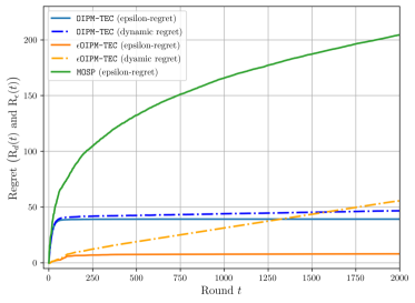
Figure 1: Regret comparison of OIPM-TEC, $\epsilon$OIPM-TEC, and MOSP

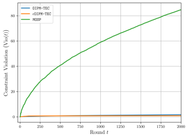
Figure 2: Constraint violation comparison of OIPM-TEC, $\epsilon$OIPM-TEC, and MOSP

5 Conclusion

In this work, an online optimization algorithm using an interior-point method-like update capable of solving the online OPF is presented. This algorithm, the OIPM-TEC, admits time-varying equality constraints and generalized inequalities while possessing a $O(V_{T}+1)$ dynamic regret bound and a $O(V_{\mathbf{b}})$ constraint violation bound. Additionally, if there exists an acceptable tolerance when solving an online optimization problem, the $\epsilon$OIPM-TEC algorithm is capable of ensuring the tightest possible bound with respect to $T$ on regret and constraint violation. These two algorithms are applied to an online OPF example showcasing their performance compared to other methods from the literature.

The possibility of using OCO approaches to solve the OPF bridges the gap between traditional OCO algorithms with performance guarantees and real-time OPF approaches like [25] and [26] that enjoy good real-world performance. A possible future direction is the development of online primal-dual interior-point methods which could increase numerical stability.

References

References

- [1] X. Cao, J. Zhang, and H. V. Poor, “A virtual-queue-based algorithm for constrained online convex optimization with applications to data center resource allocation,” IEEE Journal of Selected Topics in Signal Processing, vol. 12, no. 4, pp. 703–716, 2018.
- [2] E. Hazan, “Introduction to online convex optimization,” Foundations and Trends® in Machine Learning, vol. 2, no. 3-4, pp. 157–325, 2015.
- [3] Z. Wang, W. Wei, J. Z. F. Pang, F. Liu, B. Yang, X. Guan, and S. Mei, “Online optimization in power systems with high penetration of renewable generation: Advances and prospects,” IEEE/CAA Journal of Automatica Sinica, vol. 10, no. 4, pp. 839–858, 2023.
- [4] A. Lesage-Landry, H. Wang, I. Shames, P. Mancarella, and J. A. Taylor, “Online convex optimization of multi-energy building-to-grid ancillary services,” IEEE Transaction on Control Systems Technology, 2019.
- [5] S. Shalev-Shwartz, “Online learning and online convex optimization,” Foundations and Trends® in Machine Learning, vol. 4, no. 2, pp. 107–194, 2012.
- [6] M. Zinkevich, “Online convex programming and generalized infinitesimal gradient ascent,” in Proceedings of the 20th international conference on machine learning (icml-03), 2003, pp. 928–936.
- [7] J. Mulvaney-Kemp, S. Park, M. Jin, and J. Lavaei, “Dynamic regret bounds for constrained online nonconvex optimization based on Polyak-Lojasiewicz regions,” IEEE Transactions on Control of Network Systems, pp. 1 – 12, 2022.
- [8] E. C. Hall and R. M. Willett, “Online convex optimization in dynamic environments,” IEEE Journal of Selected Topics in Signal Processing, vol. 9, no. 4, pp. 647–662, 2015.
- [9] T. Chen, Q. Ling, and G. B. Giannakis, “An online convex optimization approach to proactive network resource allocation,” IEEE Transactions on Signal Processing, vol. 65, pp. 6350–6364, 2017.
- [10] S. H. Low, “Convex relaxation of optimal power flow—part I: Formulations and equivalence,” IEEE Transactions on Control of Network Systems, vol. 1, no. 1, pp. 15–27, 2014.
- [11] J. Kardoš, D. Kourounis, O. Schenk, and R. Zimmerman, “Beltistos: A robust interior point method for large-scale optimal power flow problems,” Electric Power Systems Research, vol. 212, p. 108613, 2022.
- [12] J. A. Taylor, Convex optimization of power systems. Cambridge University Press, 2015.
- [13] J. A. Taylor, S. V. Dhople, and D. S. Callaway, “Power systems without fuel,” Renewable and Sustainable Energy Reviews, vol. 57, pp. 1322–1336, 2016.
- [14] F. Zohrizadeh, C. Josz, M. Jin, R. Madani, J. Lavaei, and S. Sojoudi, “A survey on conic relaxations of optimal power flow problem,” European Journal of Operational Research, vol. 287, no. 2, pp. 391–409, 2020.
- [15] H. Liu, X. Xiao, and L. Zhang, “Augmented langragian methods for time-varying constrained online convex optimization,” arXiv preprint arXiv:2205.09571, 2022.
- [16] Q. Liu, W. Wu, L. Huang, and Z. Fang, “Simultaneously achieving sublinear regret and constraint violations for online convex optimization with time-varying constraints,” Performance Evaluation, vol. 152, 2021.
- [17] H. Yu and M. J. Neely, “A low complexity algorithm with O() regret and O(1) constraint violations for online convex optimization with long term constraints,” Journal of Machine Learning Research, vol. 21, no. 1, pp. 1–24, 2020.
- [18] D. J. Leith and G. Iosifidis, “Penalized ftrl with time-varying constraints,” in Machine Learning and Knowledge Discovery in Databases, M.-R. Amini, S. Canu, A. Fischer, T. Guns, P. Kralj Novak, and G. Tsoumakas, Eds. Cham: Springer Nature Switzerland, 2023, pp. 311–326.
- [19] X. Cao and K. J. R. Liu, “Online convex optimization with time-varying constraints and bandit feedback,” IEEE Transactions on Automatic Control, vol. 64, pp. 2665–2680, 2018.
- [20] M. J. Neely and H. Yu, “Online convex optimization with time-varying constraints,” 2017.
- [21] J. D. Abernethy, E. Hazan, and A. Rakhlin, “Interior-point methods for full-information and bandit online learning,” IEEE Transactions on Information Theory, vol. 58, no. 7, pp. 4164–4175, 2012.
- [22] P. Sharma, P. Khanduri, L. Shen, D. J. Bucci, and P. K. Varshney, “On distributed online convex optimization with sublinear dynamic regret and fit,” in 2021 55th Asilomar Conference on Signals, Systems, and Computers, 2021, pp. 1013–1017.
- [23] A. Lesage-Landry, J. A. Taylor, and I. Shames, “Second-order online nonconvex optimization,” IEEE Transactions on Automatic Control, vol. 66, no. 10, pp. 4866–4872, 2021.
- [24] J.-L. Lupien and A. Lesage-Landry, “An online newton’s method for time-varying linear equality constraints,” IEEE Control Systems Letters, vol. 7, pp. 1423–1428, 2023.
- [25] Y. Tang, K. Dvijotham, and S. Low, “Real-time optimal power flow,” IEEE Transactions on Smart Grid, vol. 8, no. 6, 2017.
- [26] E. Dall’Anese and A. Simonetto, “Optimal power flow pursuit,” IEEE transactions on Smart Grid, vol. 9, no. 2, 2018.
- [27] M. Picallo, L. Ortmann, S. Bolognani, and F. Dörfler, “Adaptive real-time grid operation via online feedback optimization with sensitivity estimation,” Electric Power Systems Research, vol. 212, p. 108405, 2022.
- [28] S. Boyd and L. Vandenberghe, Convex Optimization. Cambridge University Press, 2004.
- [29] J. Renegar, A Mathematical View of Interior-Point Methods in Convex Optimization. Society for Industrial and Applied Mathematics, 2001.
- [30] R. D. Zimmerman, C. E. Murillo-Sánchez, and R. J. Thomas, “Matpower: Steady-state operations, planning, and analysis tools for power systems research and education,” IEEE Transactions on Power Systems, vol. 26, no. 1, pp. 12–19, 2011.