Easing the equilibration of spin systems with quenched disorder in Population Annealing by topological-defect-driven non-local updates

Abstract

Population Annealing, the currently state-of-the-art algorithm for solving spin-glass systems, sometimes finds hard disorder instances for which its equilibration quality at each temperature step is severely damaged. In such cases one can therefore not be sure about having reached the true ground state without vastly increasing the computational resources. In this work we overcome this problem by proposing a quantum-inspired modification of Population Annealing. Here we focus on three-dimensional random plaquette gauge model which ground state energy problem seems to be much harder to solve than standard spin-glass Edwards-Anderson model. In analogy to the Toric Code, by allowing single bond flips we let the system explore non-physical states, effectively expanding the configurational space by the introduction of topological defects that are then annealed through an additional field parameter. The dynamics of these defects allow for the effective realization of non-local cluster moves, potentially easing the equilibration process. We study the performance of this new method in three-dimensional random plaquette gauge model lattices of various sizes and compare it against Population Annealing. With that we conclude that the newly introduced non-local moves are able to improve the equilibration of the lattices, in some cases being superior to a normal Population Annealing algorithm with a sixteen times higher computational resource investment.

I Introduction

Spin-glass models and, more generally, spin systems with quenched disordered interactions, consist of a set of particles or nodes, each taking a value from a range of possibilities (binary in case of the Ising models [1]) with randomly valued interactions between them, where the topology of the connections can be arbitrarily complex. Due to spin frustration and randomness such models exhibit tremendously rich behaviors and have long been one of the main focuses of statistical physics. Analytically challenging even at the mean-field level [2] and numerically hard for non-planar topologies [3], their study continues to rely mostly on numerical simulations.

In the last decades, spin-glass models have proven useful beyond their applications in physics, for example as models related to the behavior of neural networks [4, 5] and to the real-world optimization problems, especially for those that accept a Quadratic Unconstrained Binary Optimization (QUBO) mapping [6, 7]. In the QUBO picture, an optimization problem is mapped to a set of binary variables such that its ground state configuration encodes the optimal solution to the original problem. QUBO mapping applications range from fields as diverse as protein folding [8, 9], to logistics [10, 11, 12] and many others, and therefore devising ways to efficiently find the ground states of spin glass models constitutes a goal of utmost importance for both scientific and industrial problems.

Many physics-inspired algorithms have been devised for that end. One way is to use standard Markov chain Monte Carlo (MCMC) methods to mimic thermal fluctuations and utilise various temperatures to explore the rugged energy landscapes of spin-glass systems. Inspired by the process of slow thermal cooling and heating in the metallurgic industry, Simulated Annealing (SA) [13] was one of the first algorithms of such type to prove its value in real-life applications already several decades ago. As an evolution of SA and taking advantage of massively parallel computing platforms such as Graphics Processing Units (GPU) available nowadays, recently proposed Population Annealing (PA) [14, 15] is an extended ensemble Monte Carlo algorithm that combines SA’s thermal annealing with a population of independent replicas of the system under study. Thermal annealing is then significantly sped up by replicas population resampling procedure done according to the Gibbs distribution. For thermally equilibrated and sufficiently large replicas population, resampling allows to change population temperature in a single step while the population remains approximately equilibrated. This has been found to improve, in many cases, the performance of the algorithm over SA [16]. Although PA is a sequential Monte Carlo method [17] it still relies on basic a Metropolis algorithm [18] to independently equilibrate each of the replicas after every resampling step, in order to ensure that the correlations between replicas introduced by resampling are eliminated. The Metropolis algorithm is known to slowly equilibrate, e.g. in the critical region or in case of rugged landscapes [19], in which it gets trapped by local minima. The latter is problematic in spin systems with quenched disorder at low temperatures, for example when studying three-dimensional Edwards-Anderson (EA) spin-glass systems [20]. This fact can sometimes cause PA to encounter hard disorder instances for which population cannot be properly equilibrated [17]. One way to overcome the Metropolis’ algorithm deficiencies is to use cluster moves. In case of uniform, ferromagnetic, Ising models the celebrated Swendsen-Wang [21] and Wolff algorithms [22] work very efficiently. The case of spin-glass models is more problematic as clusters may grow fast, potentially spanning the whole lattice. The Houdayer cluster algorithm [23] of isoenergetic moves was designed specifically for those models. It offers substantial speed up in two dimensions and it has recently been efficiently adapted in three dimensions (and other connection topologies), even though only in specific temperature and frustration windows [24]. Therefore the search for finding efficient cluster moves in Monte Carlo algorithms for spin-glass models, especially moves compatible with massively parallel computations, remains an important challenge.

On the other hand, while the new advances on Quantum Annealing (QA) machines [25, 26] pose them as firm contenders to efficiently solve these kind of QUBO problems, they’re still far away from surpassing classical computation. As a counterpart, new quantum-inspired algorithms for classical computers have been recently developed, taking advantage from current dominant position of such platforms. Simulated Quantum Annealing (SQA) [27] constitutes the paradigmatic example within this field, in which a classical simulation of the adiabatic transition of a wave function from the initial state to the ground state of the spin-glass model is performed. In this case, the simulation of a coherent exploration of the Hilbert space upon changing Hamiltonian replaces the simulation of thermal annealing.

In this work we propose a new quantum-inspired method to improve the exploration of the optimization and quenched disorder spin problems in PA, by the evolution (annealing) of certain local constrains. Taking inspiration from the quantum Toric Code [28], the creation, movement and annihilation of topological defects within the lattice allows for the conduction of non-local moves. In two dimensions such moves can be performed on the standard spin-glass random-bond Ising model with an expanded configurational space (i.e. allowing for topological defects) and are equivalent to cluster updates. In three dimensions we propose a numerically hard model, equivalent to the random 3d random plaquette gauge model (RPGM) [29], which expanded configurational space allows for respective topological defects and non-local moves, even though the analogy with the spins clusters is not that straightforward. The evolution of such defect states starts with relaxed constrains (free defect creation) and is controlled externally by the increase of a field parameter added into the original Hamiltonian that progressively penalizes their proliferation. The preparation of the starting thermally equilibrated replica population is straightforward in any temperature as defect constrains are relaxed. Therefore annealing can be now conducted starting from any temperature, and can be performed in a two-dimensional parameter space (temperature and defect control parameter). In this regard we define an adaptive step procedure that is able to optimize the annealing of the system in this parameter space, gaining flexibility over PA, which is seen to increase the thermalization of the systems without compromising other related and desired properties. Importantly, the proposed method is itself a variation of PA, and is therefore massively parallelizable as well, leading to parallelizable effective non-local moves.

One should note that an efficient general solution to the numerically hard (NP-complete in the worst scenario) spin-glass and optimization problems, with increasing lattice sizes, is most probably impossible on classical computers. Yet even for systems and lattice sizes amenable for current computational resources, the hard disorder cases are the limiting factor. Different annealing methods (temperature in PA, adiabatic wave function changes in SQA, topological defect constrains in the present variation of PA) have the potential to address different hard disorder cases. Indeed that is what we observe: disorder cases that are difficult for standard PA are usually not that hard in our Defect-driven PA.

The paper is organized as follows. In Section II we first give a description of PA and discuss a metric for the confidence of the solution found corresponding to the global minimum, which will eventually allow us to compare the newly proposed method. We then introduce the random 3d Ising gauge theory model in plaquette representation that we named Random Field Wall (RFW) model and describe its topological defects dynamics, to finally propose the Defect-driven Population Annealing (DPA) modification. In Section III we first discuss the hardness of the RFW model and compare it against the EA one, apply DPA to RFW lattices of linear sizes $L=4,6,8$, and compare the results against the state-the-art PA algorithm. Finally, we conclude this work with a discussion in Section IV.

II Methodology

II.1 Population Annealing

Population Annealing is a generalized ensemble extension of SA in which a family of a total of $R_{0}$ replicas of the same system are independently simulated in parallel. PA starts considering all $R_{0}$ replicas at infinite temperature, at which equilibration is easy but encountering the global ground state is difficult, and anneals the population towards a low temperature at which equilibration is difficult but the probability of finding the ground state is higher. We denote the annealing schedule as $S_{\beta}=[\beta_{0},...,\beta_{N_{T}}]$, with $\beta$ the inverse temperature and $\beta_{i}<\beta_{i+1}$ $\forall i$, where $i$ labels each resampling and equilibrating step. Equilibration of the replicas is performed through a Markov Chain Monte Carlo (MCMC) method for a number of sweeps $N_{\rm{sweeps}}$, and then the population is resampled according to the Gibbs distribution, which is known to enhance the efficiency of the algorithm compared to SA. This resampling step includes elimination and proliferation of replicas that somewhat resembles the selection part of a genetic algorithm, in which replicas with a lower energy (that is, better fitness) are set to have several offspring, while those having a higher one tend to be eliminated. When resampling from an inverse temperature $\beta$ to $\beta^{\prime}$, the normalized weight for replica $j$ is defined as

$$\tau_{j}(\beta,\beta^{\prime})=R_{0}\frac{e^{-(\beta^{\prime}-\beta)E_{j}}}{\sum_{r}e^{-(\beta^{\prime}-\beta)E_{r}}},$$ (1)

where $R_{0}$ is the initial number of replicas of the system and the index $r$ runs over all replicas, and we choose its number of descendants $n_{j}$ as

$$n_{j}=\begin{cases}\left\lceil{\tau_{j}}\right\rceil&\quad\text{with probability }P_{\rm{ceil}}=\tau_{j}-\left\lfloor{\tau_{j}}\right\rfloor\\ \left\lfloor{\tau_{j}}\right\rfloor&\quad\text{with probability }P_{\rm{floor}}=1-P_{\rm{ceil}}.\end{cases}$$ (2)

This choice of probability minimizes the variance of $n_{j}$ and lets the population’s size vary around a mean value $R_{0}$ with a fluctuation of $\sqrt{R_{0}}$. This choice reduces the correlation between replicas in the descendant population [17].

An additional and important advantage of PA is that it yields an estimate of the free energy of the simulated system at no additional cost. For the annealing schedule $S_{\beta}$ described above, the estimated free energy at inverse temperature $\beta_{k}$, $\tilde{F}(\beta_{k})$ is [30]:

$$-\beta_{k}\tilde{F}(\beta_{k})=N_{s}\ln 2+\sum_{i=0}^{k-1}\ln Q(\beta_{i},\beta_{i+1}),$$ (3)

where $N_{s}$ is the total number of spins in the system and $Q(\beta,\beta^{\prime})$ is the normalization factor used by PA in the computation of the resampling weights, Eq. (1):

$$Q(\beta,\beta^{\prime})=\frac{1}{R}\sum_{r}e^{-(\beta^{\prime}-\beta)E_{r}}.$$ (4)

II.2 Confidence on the solution found

Due to their heuristic nature, algorithms such as SA or PA may not reach the global, true ground state of a certain model at hand. In such cases, one has to conform with a measure of the likelihood of the solution found being a global minimum, or as close as possible to it. Specifically for PA, we can assess this likelihood by means of measuring two different parameters on the final population of the algorithm’s run. The first one, $g_{0}$, is the fraction of replicas that, in the final population, are in the same minimum energy state detected during the entire simulation, $g_{0}=N_{0}/R$, with $N_{0}$ counting the number of times that this state appears in the final stage. The second considered parameter is the effective number of surviving families $N_{\rm{eff}}$, which measures the number of replicas that have found the lowest energy state independently. The effective number of surviving families can be measured as

$$N_{\rm{eff}}=\exp[S_{f}],$$ (5)

with

$$S_{f}=-\sum\nu_{j}\log\nu_{j},$$ (6)

the family entropy and $\nu_{j}$ the fraction of replicas present at the end of the simulation that descend from replica $j$ in the initial population. Effectively, family entropy is a measure of the equilibration or thermalization of the sample [17].

In the case of PA, the only way to be sure of having found the ground state would be to use an infinitely large population or an infinitely slow annealing process. So if the size of the final population $R$ is large enough and the same lowest energy state appears frequently in thermal equilibrium, we are able to confidently state that the found configuration is the global minimum. Therefore, the higher both parameters $g_{0}$ and $N_{\rm{eff}}$ are after a simulation, the higher confidence we might have in the solution found being the global ground state of the system. The problem in PA is then to make sure that those two parameters are high enough, and particularly the latter, since it has been seen that it sometimes encounters hard instances for which thermalization is harder, and that therefore exhibit a very low final family entropy [17, 31]. In the following, we explore problems of different hardnesses, with a focus on those that PA finds the hardest to solve.

II.3 Bond and wall representations of the models and Toric code topological defects

For simplicity, consider first a standard 2d spin lattice with only nearest neighbours interactions, defined by Hamiltonian

$$H=\sum_{\langle i,j\rangle}J_{ij}s_{i}^{z}s_{j}^{z},$$ (7)

with periodic boundary conditions. We can shift to its bond representation by applying the change of variable $\sigma_{b}^{z}=s_{i}^{z}s_{j}^{z}$:

$$H=\sum_{b}J_{b}\sigma_{b}^{z}.$$ (8)

In the bond picture of a spin lattice the new binary variables $\sigma_{b}$ represent the state of the bond between two spins, which depends on their relative alignment instead of that of the spins themselves. The bond is either said to be up (the spins connected by it have the same value, thus $\sigma_{b}^{z}=1$), or down (the spins are not aligned and $\sigma_{b}^{z}=-1$). Note that therefore a bond configuration can be translated into a spin one with up to a decision of the value of an initial spin, which corresponds to the up-down degeneracy of the spin picture.

However, in contrast to the spin representation, not all $\left\{\sigma_{b}^{z}\right\}_{b}$ configurations represent a physical state. For a bond configuration to represent a physical state of the Ising model, the products of the bonds in any close path must be 1 (see Fig. 1). To account for this we introduce plaquette and line operators:

$$B_{\square}=\prod_{b\in\square}\sigma_{b}^{z},$$ (9)

$$B_{|}=\prod_{b\in|}\sigma_{b}^{z},$$ (10)

where $b\in\square$ and $b\in|$ are the indices of the bonds pertaining to a given plaquette and line, respectively. Note that $B_{\square}$ is equivalent to TC’s $B$ operator, while the spin flip is equivalent to TC’s star operator, $A_{s}$,

$$s_{i}^{x}=\prod_{b\in+}\sigma_{b}^{x},$$ (11)

where $b\in+$ are the indices of the bonds surounding spin $s_{i}$. The condition for being able to recover a proper spin configuration translates into assuring that:

• All plaquettes yield 1.

• All straight lines across the lattice (both horizontal and vertical) yield 1.

If this condition is not fulfilled for a given plaquette or line, we say that it contains a (topological) defect (see Fig. 1). In what follows we refer to such configurations as non-physical.

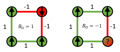
Figure 1: Physical states in the bond representation are characterized by $B_{\square}=1$. When a plaquette yields $B_{\square}=-1$, spins located on its vertices cannot be unequivocally determined and therefore the configuration does not represent a physical state of the Ising model. We thus say it contains a defect.

Let us now shift to an appropriate 3d extension of such a 2d Ising model with topological defects in bond representation. The Kramers-Wannier dual [32] to the 3d uniform Ising model is the 3d Ising gauge theory model [33] where spins are located on lattice edges and are subjected to plaquette interactions on each cube face. The latter model can be represented as a "wall model" where the walls are the new binary variables taking values of cube face plaquettes, the plaquette interaction $J$ is now a field acting on walls, and walls are not independent variables but are subjected to the constrain that in each cube the product of all 6 planes must equal 1. The given configuration of walls determines energy and represents all $2^{N}$ gauge-equivalent states (where $N$ is the number of vertices), thus in this representation entropy is greatly reduced. To visualize the 3d wall model consider an extrusion onto the new dimension of the elements of the 2d bond model described so far. This means that we add an extra dimension to all of them, and therefore degrees of freedom change as

• Spins (points) become edge spins (lines).

• Bonds (lines) become walls (planes).

And with respect to operators (constrains)

• Plaquettes (which may contain a defect) become cubes (which may contain a defect).

• Lines (which may contain a defect) become planes (which may contain a defect).

As we previously had a total of 4 spins connected by bonds (each bond connecting two single spins) and forming a plaquette surrounded by 4 bonds that could have a defect in it, we now have 12 edge spins connected by walls (each wall connecting four edges) and all of them forming a cube surrounded by 6 walls that can contain a defect as well (see Fig. 2). In this case, the change of variable between edge spin and wall models is

$$\eta_{w}^{z}=e_{i}^{z}e_{j}^{z}e_{s}^{z}e_{t}^{z},$$ (12)

where $e_{\{i,j,s,t\}}$ are the edge spins surrounding wall $\eta_{w}$.

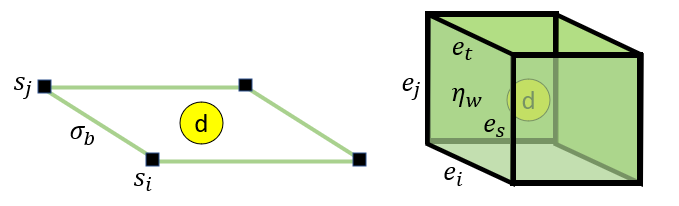
Figure 2: The 3d Random Field Wall (RFW) model is a generalization of the random 2d bond model. By extruding a plaquette and all its elements onto an extra dimension, we obtain a cube surounded by edge spins which are 4-to-4 connected by a wall. The site enclosed inside the cube can hold a defect.

Plaquette and line operators translate to cube and plane operators as

$$B_{c}=\prod_{w\in c}\eta_{w}^{z},$$ (13)

$$B_{p}=\prod_{w\in p}\eta_{w}^{z},$$ (14)

respectively and, again, the physicality of the lattice is imposed by $B_{c}=1$ $\forall c$ and $B_{p}=1$ $\forall p$. In Eqs. (13) and (14), $w\in c$ and $w\in p$ are the indices of the walls defining the cube $c$ and the plane $p$, respectively. If we now consider quenched disorder signs of plaquette interactions in 3d Ising gauge model we get the 3d random plaquette gauge model, which appeared recently in a study of stability of topological quantum memory [29] based on the TC. Following Monte Carlo simulations revealed that small concentration of negative sign plaquettes drives such system from the "Higgs phase" to the disordered "confining phase" [34, 35]. Furthermore, the phase structure of the 3d RPGM model was studied using Wu-Wang duality [36]. Here we study 3d random plaquette gauge model with Gaussian disorder for plaquette interactions in the "wall model" representation that we named 3d Random Field Wall (RFW) model. This model is not dual to the 3d Edwards-Anderson spin-glass model (also called random-bond Ising model), which consists of up/down spins arranged in a cubic lattice with only nearest-neighbor couplings, whose values are drawn from a normal distribution. In fact 3d RFW relation to the spin-glass physics is unclear. Replica symmetric mean-field solutions for random gauge theories [37] predict occurrence of "gauge-glass" phase although probably realized in higher dimensions. Still, we found the problem of finding the ground state of the 3d RFW model to be numerically hard (harder than 3d Anderson-Edwards spin-glass model for typical disorder case) and therefore suitable for testing PA and our algorithm. Finally, we note that the original 2d spin lattice can be seen as a special case of a 3d RFW lattice with a single layer of cubes, and in which we restrict the spin and wall flips to those perpendicular to the lattice plane.

II.4 Defects dynamics

Besides the usual spin-flip movement, Eq. (11) (and Eq. (15) for the 3d case, see below), we can now introduce TC topological defects into the lattice by allowing single-bond (-wall) flips with the operator $\sigma_{b}^{x}$ ($\eta_{w}^{x}$), thus extending the configurational space beyond the one representing physically feasible solutions. Note that this operator not only can create a pair of defects but can also make them move independently of each other around the lattice and eventually annihilate them if they happen to collide. This defect propagation introduces cluster-based, non-local dynamics into the MCMC simulation: if the pair of defects created follow a longer closed path until they collide, all the spins enclosed in it are effectively updated as a cluster, since all surrounding bonds have been updated (see an example in Fig. 3).

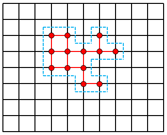
Figure 3: Allowing single-bond flips enables cluster, non-local updates in the lattice. By applying single bond-flips, a pair of defects can be created and moved around the lattice. When they collide and annihilate, the closed path they have followed (blue line) effectively realizes a non-local cluster update of the spins it encloses (red dots). The inner bonds are left unchanged in such update.

From this perspective, the spin flip operator can be seen as creating a pair of defects and moving them around a given spin (vertex), see Fig 4. Analogously to the 2d case, for the RFW the edge spin flip consists of updating all walls surrounding a given edge-spin

$$e_{\mu}^{x}=\prod_{w\in+}\eta_{w}^{x},$$ (15)

where $w\in+$ are indices of the walls located around the edge spin $\mu$.

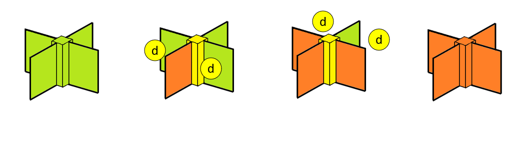
Figure 4: Graphical representation of an edge spin flip. Green and orange colors label $\pm 1$ values for the walls and the edge spin, while yellow means that there are defects in the adjacent cubes and therefore the edge cannot be unequivocally determined.

II.5 Defect-driven Population Annealing

We are now ready to introduce our algorithm, which combines PA’s features with the non-local cluster updates discussed before. We refer to this modification as Defect-driven Population Annealing (DPA). To this aim, we introduce an additional field parameter $\kappa$, with which we control the appearance of defects in the lattice by assigning an energy penalty to each of these generated defects. First of all, note that at any time we can count the number of cube and plane defects within a lattice, $N_{c}^{(D)}$ and $N_{p}^{(D)}$, with the help of operators Eq. (13) and Eq. (14), as

$$N_{c}^{(D)}=N_{c}-\sum_{c}B_{c},$$ (16)

$$N_{p}^{(D)}=N_{p}-\sum_{p}B_{p},$$ (17)

where the summations run over all cubes and all planes in the lattice, and $N_{c}$ and $N_{p}$ are the total number of cubes and planes, respectively. Accounting for this penalty the Hamiltonian reads

$$H=\sum_{w}J_{w}\eta_{w}^{z}+\kappa\left[\left(N_{c}-\sum_{c}B_{c}\right)+\left(N_{p}-\sum_{p}B_{p}\right)\right].$$ (18)

By initializing the simulation at $\kappa=0$ we ensure that the system can be readily thermalized at any chosen temperature and acquires a lot of defects. On the other hand, by changing the value of $\kappa$ to high values, at the final stages of the annealing process those configurations containing defects are penalized and rare. The configurations without defects correspond to the physical configurations of the model we want to solve. As in PA, we run the simulation on a population of $R_{0}$ independent replicas, and at each step in the annealing schedule we let them evolve with an MCMC procedure to ensure thermal equilibration, after which a resampling step is also carried out. Since at every resampling step both $\beta$ and $\kappa$ are updated, the normalized weights now are

$$\tau_{j}(\beta,\beta^{\prime},\kappa,\kappa^{\prime})=R_{0}\frac{e^{-[\beta^{\prime}E_{j}(\kappa^{\prime})-\beta E_{j}(\kappa)]}}{\sum_{r}e^{-[\beta^{\prime}E_{r}(\kappa^{\prime})-\beta E_{r}(\kappa)]}},$$ (19)

with $E(\kappa)=\sum_{w}J_{w}\eta_{w}+\kappa[N_{c}^{(D)}+N_{p}^{(D)}]$.

II.5.1 Family entropy-preserving annealing

As have been discussed, a bad thermalization of the system is characterized by a low final value of family entropy, which is reduced everytime a resampling step is carried on the population. In standard Population Annealing, in which a linear schedule in $\beta$ is classically used in the literature, the family entropy tends to follow a geometric decay, Fig. 5. Instead, in order to maximize its value during the whole simulation, we propose to adapt the annealing process such that, at each resampling step, a constant portion of the number of surviving families is lost. This way the family entropy follows an exponential decay towards an objective value, which we can tune externally. To this end we implement an adaptive step procedure for both annealing schedules, $S_{\kappa}$ and $S_{\beta}$. Before each resampling step $(\beta,\kappa)\to(\beta^{\prime},\kappa^{\prime})$, we compute the optimal values of $\kappa^{\prime}$ and $\beta^{\prime}$ such that the obtained family entropy follows the specified decay

$$\frac{N_{\rm{eff}}(t_{n})}{R_{0}}=\left(\frac{N_{\rm{eff}}^{\rm{desired}}}{R_{0}}\right)^{\frac{t_{n}}{N_{T}}},$$ (20)

where $t_{n}$ is the simulation step, $N_{\rm{eff}}(t_{n})$ is the number of surviving families at that time, and $N_{\rm{eff}}^{\rm{desired}}$ is the objective number of surviving families at the end of the simulation.

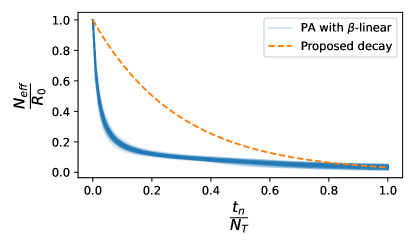
Figure 5: Entropy-preserving annealing. Comparison between the decay in family entropy obtained in PA simulations of $L=4$ RFW lattices with a $\beta$-linear annealing schedule (blue lines) and the objective, implemented decay (orange line). Each blue line is the decay obtained for a different disorder. Although final family entropy may seem very similar in this scale, its fluctuations in PA simulations describe differences between hard and easy disorder cases.

One can intuitively see that $g_{0}$ and the final $N_{\rm{eff}}$ can be somewhat interchanged, as each resampling step may eliminate replicas with high energy values from independent families in order to replicate a more optimal one. As we shall see later, the drive through the two-dimensional $(\beta,\kappa)$-space allows the system to minimize the loss of surviving families, yielding values on the upper section of the range of the blue lines in Fig. 5, while still maximizing the final $g_{0}$. This will happen to be achievable even for these hardest cases for which PA does not properly equilibrate the population and thus yields a negligible family entropy. However, if a too ambitious final objective family entropy is set, it might come at the cost of a large loss of $g_{0}$. In that case, an extra resampling step at a very low temperature can be applied, such that we trade one for the other by effectively replicating those states with the lowest energy.

II.5.2 Remaining defects

It may happen that only annealing through $\kappa$ is not enough to ensure that we get rid of the defects at the end of the simulation and that some of them get stuck in potential traps, thus ending up with physically unfeasible lattices. In such cases two additional procedures can be applied. On the one hand, an N-fold way algorithm [38] among the already existing defects only (thus they can be moved and annihilated, but no new defects can be created) is used to increase their mobility and speed up their dynamics. On the other hand, an attraction potential between defects can be used to reduce the probability of them getting stuck inside potential traps while forcing them to collide. This is done by the introduction into Hamiltonian Eq. (18) of the additional term

$$H_{G}=G\sum_{i=1}^{N_{\rm{def}}}{\sum_{j=0}^{i-1}{\frac{1}{D_{ij}^{\alpha}}}},$$ (21)

where $G$ is a negative constant that can be tuned, $N_{\rm{def}}$ is the number of defects present in the lattice, $D_{ij}$ is the euclidean distance between defects at sites $i$ and $j$, and $\alpha$ can be used to make the interaction potential shorter or longer ranged.

III Results

III.1 Hardness of the RFW model

One of the standard and most widely used spin glass models is the so-called Edwards-Anderson model [20], for which reliable results on its 3-dimensional version have been reported for sizes of up to $L=10$ [16], or equivalently, a total of $N_{s}=1000$ spins. Bigger lattice sizes have also been explored in the literature, but with a lower degree of confidence on the quality of the thermalization achieved [17]. As discussed earlier, the RFW model does not correspond to the standard 3d-EA model but allows for the effective dynamics of topological defects. This model is, as we show below, much more difficult to solve for typical disorder cases as much more computational resources must be used in order to properly thermalize it. This difference in computational hardness can be seen straightforwardly when standard PA is used by measuring the free energy of the system. The free energy is given by $F=E_{0}-TS$, where $E_{0}$ is the energy of the global ground state of the system, $T$ is the temperature and $F$ and $S$ are the free energy and the entropy of the system at that temperature, respectively. At temperatures sufficiently low (both $T$ and $S$ close to 0), the free energy and the ground-state energy will coincide and thus their ratio will approach 1. Alternatively, a ratio close to 1 serves as a hint that the global ground state has been found and that the model has been properly thermalized at low temperatures.

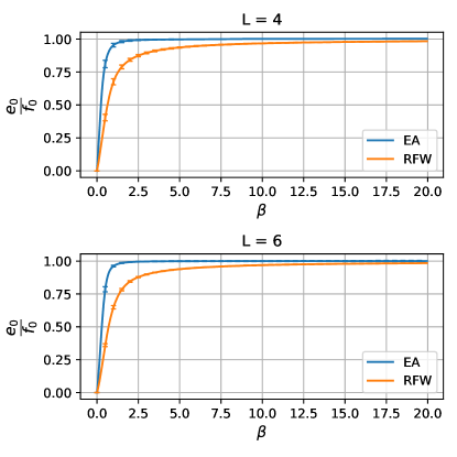
Figure 6: RFW models are computationally harder than their EA counterparts. Comparison of the ratio between the minimum energy found and the estimated free energy, at a given $\beta$ during a simulation, for EA and RFW models. Solid lines indicate the average among 100 different disorder realizations and error bars indicate the standard deviation of such disorders over their average. Lattice sizes of $L=4$ (top panel) and $L=6$ (bottom panel).

We solve 100 different disorder realizations of the EA and RFW models for $L=4$ and $L=6$ with PA and keep track of the ratio ${}^{E_{0}}\!/_{\tilde{F}}$ as a function of the inverse temperature. For a fair comparison, we used the same computational resources and the same annealing schedule for both models. We plot the disorder-averaged results in Fig. 6, where at each point the ratio is calculated with the minimum energy found until then, $e_{0}$ and the free energy estimate at that temperature given by PA, $f_{0}$. The rather small error bars represent the standard deviation of the individual lines over the mean, indicating that there is little variability between different disorders for both EA and RFW models. There is also little difference when comparing lattice sizes of the same model, although the curve for RFW appears to be consistently quite lower than that for EA. Concretely, we see that $\beta=5$ seems to be more than enough to confidently state that PA has found the global ground state for both lattice sizes of the EA model, while going to $\beta=20$ (and therefore using up to four times more computational time) still does not yield a convincing ratio for the RFW model.

Furthermore, we also take a look at the PA’s acceptance ratio of MC updates for various instances of both models as a function of the inverse temperature $\beta$, Fig. 7. We observe that $\beta=5$ seems to be a sufficiently low temperature for both models, since the acceptance ratio is already very low ($\beta=5$ is the standard value used in the literature to solve the EA model [17], and the values are even higher than those obtained for RFW lattices). We nonetheless check and confirm that for RFW the minimum energy found during the whole simulation is the exact same one already found at $\beta=5$, which means that from then on the only factor improving the results is the resampling of the population. Combining the results shown in Figs. 6 and 7 we conclude that the increase in ${}^{e_{0}}\!/_{f_{0}}$ with high values of $\beta$ observed for the RFW lattice model can only be due to the decrease of the $TS$ term, which means that this model has much more entropy at lower temperatures and therefore is more difficult to thermalize. This entropy is not related to the gauge freedom of the underlying 3d RPGM as the wall representation removed it. Rather it is perhaps related to the non-ordered nature of the "confining phase" in 3d RPGM versus the spin-glass order in the 3d EA model.

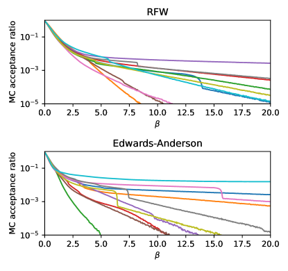
Figure 7: RFW and EA models have similar MC acceptance ratios when solved using the PA algorithm. Population annealing’s acceptance ratios of MC updates for different disorders of RFW lattices (top panel) and Edwards-Anderson lattices (bottom panel), as a function of inverse temperature $\beta$. Each line is the result obtained for a different disorder.

Another way we can take a look at the comparably much greater difficulty of the RFW model is by reducing the spin frustration created by the disorder by tuning the ratio of negative-valued bonds it contains. To do so, we generate normal Gaussian distributions, take their absolute value and change the sign of a randomly selected portion of them. The lower the ratio of negative bonds that the disorder instance has, the lesser the amount of frustrated spins it can potentially have, and thus the easier it will be to find its minimum energy configuration, eventually reaching the trivial limit of a ferromagnetic disorder. We consider three different ratios of negative bonds, $r_{nb}=\{0.25,0.10,0.02\}$ and solve a total of 1000 disorder instances of RFW lattices of size $L=4$ for each of them with PA. In the top panels of Fig. 8 we show the histograms of the measured parameters discussed in previous sections, $g_{0}$ and ${}^{N_{\rm{eff}}}\!/_{R_{0}}$ for such cases, along with those obtained for unbiased Gaussian disorders (equivalent to $r_{nb}=0.5$) and those obtained for $L=4$ lattices under the Edwards-Anderson model. Again, we use the same parameters for all of them. In the center panels of Fig. 8 we plot the dependence of the mean values of such histograms with $r_{nb}$, with error bars showing its standard deviations. We observe how the histograms tend to shift to higher values for smaller $r_{nb}$ and therefore for easier disorders.

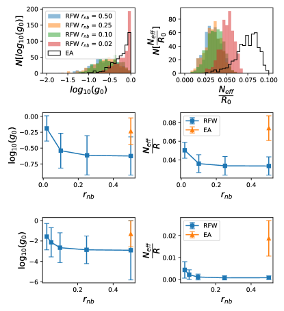
Figure 8: The hardness of RFW models against EA clearly emerges when varying the frustration level of the solved lattices. Top panels: histograms of $g_{0}$ and ${}^{N_{\rm{eff}}}\!/_{R_{0}}$ obtained for $L=4$ RFW lattices of various ratio of negative bonds, $r_{nb}$, along with the ones obtained for Edwards-Anderson lattices. Center panels: mean values and standard deviations of such histograms, as a function of $r_{nb}$. Bottom panels: mean values with standard deviations of the same histograms but for $L=6$ lattices. All simulations are obtained with PA with the same set of parameters. Legends in left and right panels are the same but are not shown to improve visibility of the plots.

We highlight two main consequences from the results shown in Fig. 8. On the one hand, we confirm that, as discussed earlier, higher values of $g_{0}$ and the family entropy are correlated with higher confidence in the solution found being the global ground state and, therefore, can be used as a metric to this end. On the other hand, it shows how strikingly harder the RFW model is compared to typical Edwards-Anderson instances with uncorrelated disorders, obtaining comparable values of $g_{0}$ only when restricting the frustration of disorders to a ratio of negative bonds of about $2\%$, while still getting much worse values for the family entropy. Looking at the same curves for $L=6$, we observe pretty similar results, bottom panels of Fig. 8. Although the $g_{0}$ obtained for the EA model is approximately equal to the one obtained for RFW with about $2\%$ negative bonds, the family entropy is still far from it even for such low-frustration cases. It is also worth noting that, for $L=6$, this difference is even greater than for $L=4$.

Further, we implement $L=8$ RFW lattices with Gaussian disorder ($r_{nb}=0.5$), and attempt to solve them with standard PA using a large amount of computational resources. For equally large EA lattices, the parameter set $(R_{0},N_{T},N_{\rm{sweeps}})=(5\cdot 10^{5},200,10)$ is reported to be more-than-adequate resources in [16], where $R_{0}$ is the initial population size, $N_{T}$ is the number of temperatures in the annealing schedule and $N_{\rm{sweeps}}$ is the number of sweeps carried on per temperature (each sweep consists of attempting $N_{\rm{spins}}$ MC updates on the lattice). For comparison, in our simulations we used $(R_{0},N_{T},N_{\rm{sweeps}})=(2.6\cdot 10^{5},500,20)$ and repeatedly solved 20 different disorder realizations in order to see how many times the algorithm converged to the same minimum energy state. Among all of them, the convergence ratios between independent runs varied from a minimum of $0\%$ (in 11 out of the 20 studied disorders) to a maximum of $12\%$ (in only three of them).

In light of these conclusions about the hardness of the present model, in what follows we restrict ourselves to a thorough study of RFW lattices of $L=4$ and $L=6$ with purely Gaussian disorders (this is, $r_{nb}=0.5$). Finally, we present some preliminary results for $L=8$ lattices as well.

III.2 Comparison between PA and DPA

In order to gain an insight into how the different algorithms perform, we solve, for each lattice size, several disorders with couplings randomly drawn from a Gaussian distribution and compare the obtained $g_{0}$ and $N_{\rm{eff}}$. For a fair comparison, we should spend the same amount of computational work $W$ on both PA and DPA simulations. For that, we define the computational work $W$ as the total number of MCMC updates attempted during a simulation, namely

$$W=N_{\rm{sweeps}}N_{T}R_{0}$$ (22)

with $N_{T}$ the total number of steps in the annealing schedule, $N_{\rm{sweeps}}$ the number of sweeps per temperature, and $R_{0}$ the initial number of replicas. Note that, as discussed above and according to Eq. (2), the population size at step $i$, $R_{i}$, fluctuates during the simulation and therefore a more accurate formula would be $W=N_{\rm{therm}}\sum_{i=0}^{N_{T}}R_{i}$. However, since we use a resampling protocol that minimizes fluctuations in population size, we can accurately approximate $R_{0}\approx N_{T}^{-1}\sum R_{i}$ and use the former. It should also be noted that the contribution of the resampling steps to the total computational work can be neglected. To study a fair comparison between both algorithms, we always use the same initial number of replicas and the same number of temperatures in the annealing schedules. In PA we implement the widely used linear in inverse temperature schedule, $S_{\beta}=[0,5]$. For the DPA simulations, after an exploration of the parameter space we found $(\beta_{0},\kappa_{0})=(0,0)$ and $(\beta_{0},\kappa_{0})=(2,0)$ to be, generally, good starting points for the entropy-preserving adaptive steps in the $L=4$ and $L=6$ cases, respectively. For $L=8$ we used $(\beta_{0},\kappa_{0})=(2,0)$ as well, even though due to long simulation times the exploration of the parameter space was not that extensive and thus this initial point is more prompt to be optimized. Our method is therefore able to thermalize the system at finite temperatures as long as $\kappa_{0}=0$, which shows it has a better plasticity over PA.

Nevertheless, since in DPA we perform one spin flip and one wall flip per iteration, we distinguish between two different measures of computational work. In the first scenario, assuming that random number generation is the main bottleneck in MC algorithms, a strictly fair comparison would impose that $N_{\rm{sweeps}}^{(PA)}=2N_{\rm{sweeps}}^{(DPA)}$, even if this evidently yields a much poorer thermalization for the former. On the other hand, if a fast enough random number generator is assumed, one can directly count the computational work as the total number of MCMC updates attempted along the simulation. As we have discussed previously, each spin flip consists of four wall flips and, conversely, each wall flip can be counted as one fourth of a spin flip. This means that, in this case, to use the same $W$ one has to impose $N_{\rm{sweeps}}^{P(A)}=\frac{5}{4}N_{\rm{sweeps}}^{(DPA)}$ (recall that each thermalization step in DPA consists of one spin flip and one wall flip, which equate to five walls being updated). We address and compare both scenarios using $N_{\rm{sweeps}}^{(PA)}=10$ and $N_{\rm{sweeps}}^{(DPA)}=5$ for the first and $N_{\rm{sweeps}}^{(PA)}=10$ and $N_{\rm{sweeps}}^{(DPA)}=8$ for the second.

III.2.1 $L=4$

We first apply the new method to the study of $L=4$ RFW lattices and take a look at the histograms of the parameters $g_{0}$ and $N_{\rm{eff}}$ obtained for 500 different disorders, comparing the solutions obtained for the same disorders with a regular PA algorithm. We plot our results in Fig. 9, the left panels corresponding to the first scenario discussed ($W$ limited by the amount of random numbers) and the right panels corresponding to the second ($W$ limited by the number of MC updates). The top graphs show the histograms for $g_{0}$, the middle graphs the histograms for ${}^{N_{\rm{eff}}}\!/_{R_{0}}$, and the bottom graphs the scatter plot relating both parameters for each of the solved disorders. In these bottom panels, we also mark the disorders that regular PA finds to be the hardest to solve, identified as those obtaining the lowest values of family entropy (red crosses) and how these same disorders score when solved by DPA (black crosses). In this case, we consider a disorder to be hard whenever PA is not able to reach a final effective number of surviving families ${}^{N_{\rm{eff}}}\!/_{R_{0}}=0.015$ or, equivalently, about 2$\%$ of all instances of disorder.

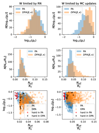
Figure 9: DPA outperforms PA for L=4 lattices when MCMC process simulations are the computational bottleneck. Histograms of $g_{0}$ and $N_{\rm{eff}}/R$ obtained by solving, by both PA and DPA, a total of $N_{\rm{dis}}=500$ different disorders of $L=4$ RFW lattices, with bonds randomly distributed according to a normal distribution. Simulations using the same amount of random numbers (left panels) and of MCMC updates (right panels). Crosses in the bottom panels mark these instances PA finds the hardest (red), and how these same instances score in DPA (black).

In the first scenario (Fig. 9, left panels) we observe a certain trade-off between parameters (Fig. 9, top left and center left panels), resulting in an equivalent performance of the two methods. The fact that the adaptive steps procedure over the two control parameter space ($\beta$, $\kappa$) is able to properly drive the evolution of the system and set an objective cutoff family entropy is nevertheless noticeable (Fig. 9, center left panel). Also, the fact that the the family entropy is no worse than for PA is relevant, taking into account that, in this scenario, the total amount of spin updates is lower and thus one might expect a worse thermalization. With the cut-off imposed on family entropy, scores on this parameter are increased even for hard cases, but they seem to lay, generally, in the lower range for DPA as well (Fig. 9, bottom left panel).

On the other hand, in the second scenario (Fig. 9, right panels) we see a substantial improvement with the DPA method, as the histograms for both measured parameters seem to be shifted towards bigger values and thus imply better metrics than those obtained with standard PA (Fig. 9, top right and center right panels). As can be seen in the bottom right panel, even some of the hard cases’ metrics are improved, as they manage to escape from the lower range of family entropy without diminishing its $g_{0}$ score.

In Fig. 10 we take a closer look at the results obtained by the two methods, by comparing the measured parameters obtained by both for each of the solved disorder realizations. A brighter color indicates a higher density of points and the red straight line is plotted to indicate the region in which both methods yield the same results for a given parameter. We also marked those disorder instances classically labeled as hard for PA with red crosses. Again, the left and right panels correspond to the first and second scenarios, respectively.

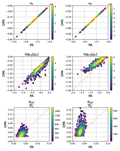
Figure 10: DPA provides on average higher family entropies than PA when solving $L=4$ lattices. Comparison of results obtained by PA and DPA for $L=4$ RFW lattices for the three measured parameters. From top to bottom: ground state energy, $g_{0}$ and effective number of surviving families. Simulations using the same amount of random numbers (left) and of MCMC updates (right).

Most importantly, as can be seen in the top panels of Fig. 10, both algorithms find the same ground state energy for all disorders. The distribution of $g_{0}$ and $N_{\rm{eff}}$ is shown in the center and bottom panels, respectively. In them we can see that for the same amount of RN consumed (first scenario, left panels) the obtained $g_{0}$ is slightly higher for PA but certainly comparable to DPA for the vast majority of disorders (Fig. 10, middle left panel), even for most of the hardest instances. On the other hand, the family entropy is better with the new method (Fig. 10, bottom left panel), which implies that a better thermalization of the replicas is achieved (again, recall that the number of total spin updates is lower, and thus this could have been expected to be lower as well). In the second scenario, DPA obtains clearly better results than PA for both parameters, $g_{0}$ (Fig. 10, middle right panel), and $N_{\rm{eff}}$ (Fig. 10, bottom right panel).

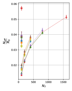
Figure 11: Hard cases on PA require more adiabatic annealing processes to reach an equivaent family entropy to DPA. Study of the amount of computational power that would have to be invested to solve $L=4$ RFW lattices with PA, in order to obtain a similar final family entropy as with DPA, for hard instance for which $g_{0}^{PA}\approx g_{0}^{DPA}$. Error bars are standard deviations over $N_{\rm{rep}}=100$ repetitions of the same process at each value of $N_{T}$. Square markers are obtained with DPA and triangle ones with PA using an increasing number of temperature steps. Each color indicates a different disorder.

Lastly, we focus on cases of disorder realizations that are hard for the PA algorithm, that is these cases resulting in low family entropy. From Eq. (1) follows that a possible way to overcome the difficulty of equilibration and improving the final family entropy obtained by PA is to reduce the differences $\Delta\beta=\beta^{\prime}-\beta$ by increasing the number of temperature steps. Following this idea, to further contrast both methods, we now take a collection of disorders that PA finds difficult to equilibrate and for which a very similar $g_{0}$ is obtained for PA and DPA, so that they lay close to the $g_{0}^{PA}=g_{0}^{DPA}$ red line in the center panels of Fig. 10, and repeatedly solve them several times with an increasing number of temperature steps in the PA annealing schedule (i.e. more adiabatically). For the cases at hand, we find that for PA to obtain a family entropy similar to that obtained by DPA, we would have to invest approximately between 4 and 16 times as much computational power depending on the disorder instance, Fig. 11. Furthermore, one should also note here that, contrary to the addition of more replicas, that extra computational effort would not be parallelizable in PA, since the annealing schedule must always be followed sequentially.

III.2.2 $L=6$

We now apply the same study to $L=6$ RFW lattices. As for the $L=4$ case, we solve several different Gaussian disorders with both PA and DPA considering the two scenarios discussed above, and plot the obtained histograms in Fig. 12. For the first scenario, (Fig. 12, left panels), we again see a certain trade-off between $g_{0}$ and $N_{\rm{eff}}$. Nevertheless, the gain in family entropy is now more noticeable than for smaller lattices, as now PA does encounter some hard instances for which it obtains a single surviving family, preventing adequate thermalization. On the contrary, the adaptive steps in DPA are capable of driving the population toward nonzero values, thus ensuring proper thermalization (Fig. 12 center left panel). When considering the computational work limited by the number of MC updates, the $g_{0}$ obtained with DPA is comparable to that obtained with PA, while the gain in family entropy remains the same. Again, those hard instances of PA are properly thermalized under DPA. On top of that, comparing the results obtained for each individual disorder between the two scenarios (Fig. 12 bottom panels), we see that, while for PA the hard instances are more or less evenly distributed along the range of $g_{0}$ values, they are shifted towards bigger values, especially for the second scenario.

Looking at the top panels of Fig. 13 we again confirm that both methods find the same ground-state energy for all disorder realizations. Speaking of $g_{0}$, the hardest instances are more or less uniformly distributed around their mean in both scenarios (Fig. 13 middle panels), while shifted towards PA when restricted by the generation of random numbers, but centered between the two methods when restricted by the amount of MC updates.

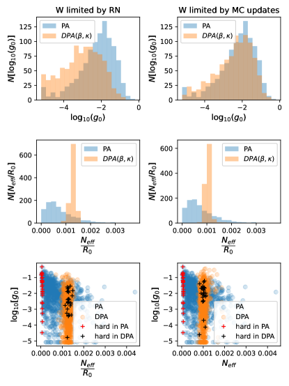
Figure 12: DPA enables thermalization of $L=6$ lattices, even when these are hard for the PA algorithm. Histograms of $g_{0}$ and $N_{\rm{eff}}/R$ obtained by solving, by both PA and DPA, a total of $N_{\rm{dis}}=1000$ different disorders of $L=6$ RFW lattices, with bonds randomly distributed according to a normal distribution. Simulations using the same amount of random numbers (left) and of MCMC updates (right). Crosses in the bottom panels mark these instances PA finds the hardest (red), and how these same instances score in DPA (black).

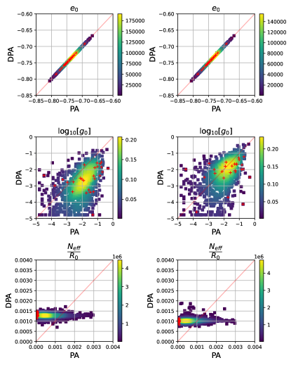
Figure 13: DPA provides on average higher family entropies than PA when solving $L=6$ lattices. Comparison of results obtained by PA and DPA for $L=6$ RFW lattices for the three measured parameters. From top to bottom: ground state energy, $g_{0}$ and effective number of surviving families. Simulations using the same amount of numbers (left) and of MCMC updates (right).

We finally study in Fig. 14, as in the case $L=4$, a collection of instances that PA finds hard and that obtain a similar value of $g_{0}$ with both methods. Again, we use an increasingly adiabatic process in PA to see how much more computational power would be necessary to get results comparable to those obtained with PA. In this case, DPA achieves an equivalent performance to PA with about between 2 and 5 more computational investment, depending on the instance. We note a more linear behaviour of the family entropy with $N_{T}$ than in Fig. 14, probably because the considered values of $N_{T}$ are not big enough. This indicates that $L=6$ is on the limit of our numerical capabilities.

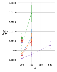
Figure 14: Hard cases on PA require more adiabatic annealing processes to reach an equivaent family entropy to DPA. Study of the amount of computational power that would have to be invested to solve $L=6$ RFW lattices with PA, in order to obtain a similar final family entropy as with DPA, for hard instances for which $g_{0}^{PA}\approx g_{0}^{DPA}$. Error bars are standard deviations over $N_{rep}=100$ repetitions of the same process at each value of $N_{T}$. Square markers are obtained with DPA and triangle ones with PA using an increasing number of temperature steps. Each color indicates a different disorder.

III.2.3 $L=8$

In order to study hard EA disorders on big lattice sizes for which a proper thermalization is not guaranteed, one classically relies on running many times the same instance independently. We apply this methodology to $L=8$ RFW lattices with Gaussian disorder to test how both algorithms perform. Concretely, we study 20 different disorder instances and run each of them 50 times with each algorithm, considering the computational work limited by the amount of MC updates (second discussed scenario in previous sections). As the systems are not thermalized, we only focus here on the minimum energies per spin found during the simulations, $e_{min}$, and not on the previously discussed metrics. Contrarily to what should be expected from a thermalized system, none of the algorithms clearly converges to the same energy among different runs for a given disorder. In fact, when studying it with PA, for 11 out of the 20 studied cases the same minimum energy was not found in any of the runs. For 4 of them the minimum energy was found twice, for 2 of them four times and only for the 3 easiest ones it was repeatedly found six times. In Fig. 15 we show, for one of the three easy studied instances (top panel) and for one of the 11 hard ones (bottom panel), the minimum energies found among independent runs by each algorithm.

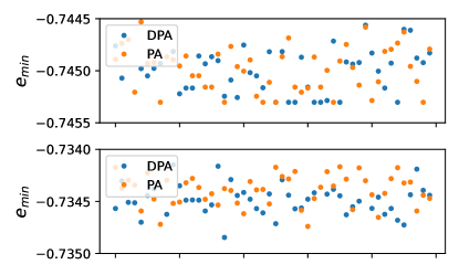
Figure 15: Both algorithms have a low convergence ratio to the same minimum energy state among independent runs. Upper panel: example of an easy case, for which both algorithms find the same solution after running it several times (both PA and DPA show a convergence ratio of $12\%$). Bottom panel: example of a hard case, for which both algorithms completely fail to converge towards any minimum energy state, and for which DPA finds the best solution between the two.

On the one hand, we observe that the spread of the minimum energies found among several runs of the same disorder tends to be larger with DPA than with PA, probably due to the larger configurational space caused by the introduction of topological defects. On the other hand, when comparing the minimum energy found with both algorithms, we observe that DPA generally performs better, yielding lower energies (see Fig. 16, the "tie" cases contain easy disorders). The fact that DPA generally finds states with lower energies when solving hard instances for which thermalization is poor (or, equivalently, for which no convergence to the same solution is achieved) indicates that the proposed non-local moves are indeed useful to explore energy landscape in hard disorder instances, effectively allowing the system escape local minima.

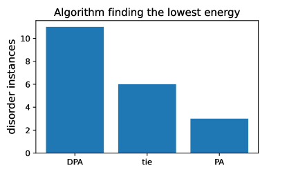
Figure 16: DPA finds lower energy states. When studying non-thermalized RFW $L=8$ lattices, DPA is generally able to find lower energies than PA using the same computational resources (in the same amount of MCMC updates scenario). Results obtained after solving 20 different disorder instances, 50 times each with each algorithm.

IV Conclusions and outlook

In this paper we introduced a method, inspired by the Toric Code, of exploring rugged energy landscape of 2d random-bond Ising and 3d random plaquette gauge models based on creation, movement and annihilation of topological defects. The advantages of this approach are: (i) from the point of view of the original phase space of the models, the effect of the dynamics of the topological defects is equivalent to non-local moves, which allow the system to overcome energy barriers that other exploration strategies based on thermal fluctuation or tunneling don’t, (ii) topological defect moves are compatible with massively parallel implementations. The disadvantage of this approach is a substantial enlargement of the phase space in the early stages of simulation.

We implemented this method in a state-of-the-art Population Annealing algorithm by adding moves related to topological defects and an extra field parameter in the Hamiltonian, $\kappa$, which energetically penalizes them. The presented Defect-driven Population Annealing (DPA) algorithm utilizes annealing in a two-parameter space: the temperature and the $\kappa$, where starting temperature may now be arbitrary. This offers additional application flexibility, but leaves the annealing path undetermined. To this end we devised a new family entropy-preserving adaptive step procedure that effectively navigates the $(\beta,\kappa)$-space in order to drive the replica population towards an objective value of final family entropy.

We have tested the new algorithm on the 3d random plaquette gauge model, as the 2d random bond Ising model lacks numerically hard disorder cases. We leave the problem of algorithm performance in 2d random bond Ising model for future study. The ground state problem of the 3d RPGM with Gaussian disorder was solved in a representation we named random field wall model, using standard PA as a benchmark. We found that the RFW model is substantially more numerically demanding than the 3d Edwards-Anderson model, which limited our thorough simulations to lattice sizes $L=4$ and $L=6$. Bigger lattices have been explored, but we leave its thorough study for a future extension of the present work. The results for DPA on those lattices have shown that it is capable of improving thermalization in comparison with PA, effectively avoiding running out of family entropy even for the hardest disorder instances. When focusing on the instances that PA finds the hardest, we have been able to observe that DPA can be superior to regular PA with a computational investment 2 to 16 times higher, approximately, depending on the case. Yet sometimes DPA trades improvement of family entropy for decrease in $g_{0}$ metric. Finally, when studying hard cases for which thermalization is not properly achieved, the proposed non-local moves still show an advantage in overcoming energy barriers and thus yield lower energies. It is also worth noting that the results are greatly improved when a fast enough random number generator is used, such that the Monte Carlo updates themselves constitute the real bottleneck for the simulations and thus the fair measure of the computational work invested.

V Acknowledgments

D.C.G. acknowledges funding from Generalitat de Catalunya (AGAUR Doctorats Industrials 2019, 2n termini). ICFO group acknowledges support from: ERC AdG NOQIA; Ministerio de Ciencia y Innovation Agencia Estatal de Investigaciones (PGC2018-097027-B-I00/10.13039/501100011033, CEX2019-000910-S/10.13039/501100011033, Plan National FIDEUA PID2019-106901GB-I00, FPI, QUANTERA MAQS PCI2019-111828-2, QUANTERA DYNAMITE PCI2022-132919, Proyectos de I+D+I “Retos Colaboración” QUSPIN RTC2019-007196-7); MICIIN with funding from European Union NextGenerationEU (PRTR-C17.I1) and by Generalitat de Catalunya; Fundació Cellex; Fundació Mir-Puig; Generalitat de Catalunya (European Social Fund FEDER and CERCA program, AGAUR Grant No. 2021 SGR 01452, QuantumCAT  U16-011424, co-funded by ERDF Operational Program of Catalonia 2014-2020); Barcelona Supercomputing Center MareNostrum (FI-2023-1-0013); EU (PASQuanS2.1, 101113690); EU Horizon 2020 FET-OPEN OPTOlogic (Grant No 899794); EU Horizon Europe Program (Grant Agreement 101080086 — NeQST), National Science Centre, Poland (Symfonia Grant No. 2016/20/W/ST4/00314); ICFO Internal “QuantumGaudi” project; European Union’s Horizon 2020 research and innovation program under the Marie-Skłodowska-Curie grant agreement No 101029393 (STREDCH) and No 847648 (“La Caixa” Junior Leaders fellowships ID100010434: LCF/BQ/PI19/11690013, LCF/BQ/PI20/11760031, LCF/BQ/PR20/11770012, LCF/BQ/PR21/11840013). Views and opinions expressed are, however, those of the author(s) only and do not necessarily reflect those of the European Union, European Commission, European Climate, Infrastructure and Environment Executive Agency (CINEA), nor any other granting authority. Neither the European Union nor any granting authority can be held responsible for them.

References

- BRUSH [1967] S. G. BRUSH, Rev. Mod. Phys. 39, 883 (1967).
- Parisi [2007] G. Parisi, “Mean field theory of spin glasses: statics and dynamics,” (2007), arXiv:0706.0094 [cond-mat.dis-nn] .
- Barahona [1982] F. Barahona, Journal of Physics A: Mathematical and General 15, 3241 (1982).
- Amit et al. [1985] D. J. Amit, H. Gutfreund, and H. Sompolinsky, Phys. Rev. A 32, 1007 (1985).
- van Hemmen [1986] J. L. van Hemmen, Phys. Rev. A 34, 3435 (1986).
- Lucas [2014] A. Lucas, Frontiers in Physics 2 (2014), 10.3389/fphy.2014.00005.
- Lucas [2019] A. Lucas, Quantum Information Processing 18 (2019), 10.1007/s11128-019-2323-5.
- Irbäck et al. [2022] A. Irbäck, L. Knuthson, S. Mohanty, and C. Peterson, Phys. Rev. Res. 4, 043013 (2022).
- Oliveira et al. [2018] N. M. D. Oliveira, R. M. D. A. Silva, and W. R. D. Oliveira, International Journal of Quantum Information 16, 1840007 (2018), https://doi.org/10.1142/S0219749918400075 .
- Hernández et al. [2020] F. Hernández, K. Díaz, M. Forets, and R. Sotelo, in 2020 IEEE Congreso Bienal de Argentina (ARGENCON) (2020) pp. 1–1.
- Phillipson and Chiscop [2021] F. Phillipson and I. Chiscop, in Computational Science – ICCS 2021, edited by M. Paszynski, D. Kranzlmüller, V. V. Krzhizhanovskaya, J. J. Dongarra, and P. M. A. Sloot (Springer International Publishing, Cham, 2021).
- Sales and Araos [2023] J. F. A. Sales and R. A. P. Araos, “Adiabatic quantum computing for logistic transport optimization,” (2023), arXiv:2301.07691 [quant-ph] .
- Kirkpatrick et al. [1983] S. Kirkpatrick, C. D. Gelatt, and M. P. Vecchi, Science 220, 671 (1983).
- Gubernatis [2003] J. Gubernatis, The Monte Carlo Method in the Physical Sciences: Celebrating the 50th Anniversary of the Metropolis Algorithm : Los Alamos, New Mexico, 9-11 June 2003 (American Institute of Physics, 2003).
- Machta [2010] J. Machta, Phys. Rev. E 82, 026704 (2010).
- Wang et al. [2015a] W. Wang, J. Machta, and H. G. Katzgraber, Phys. Rev. E 92, 013303 (2015a).
- Wang et al. [2015b] W. Wang, J. Machta, and H. G. Katzgraber, Phys. Rev. E 92, 063307 (2015b).
- Metropolis [1953] N. e. a. Metropolis, The Journal of Chemical Physics 21 (1953), 10.1063/1.1699114.
- Newman and Barkema [1999] M. E. J. Newman and G. T. Barkema, Monte Carlo methods in statistical physics (Clarendon Press, Oxford, 1999).
- Edwards and Anderson [1975] S. F. Edwards and P. W. Anderson, Journal of Physics F: Metal Physics 5, 965 (1975).
- Swendsen and Wang [1987] R. H. Swendsen and J.-S. Wang, Phys. Rev. Lett. 58, 86 (1987).
- Wolff [1989] U. Wolff, Phys. Rev. Lett. 62, 361 (1989).
- Houdayer [2001] J. Houdayer, The European Physical Journal B - Condensed Matter and Complex Systems 22, 479 (2001).
- Zhu et al. [2015] Z. Zhu, A. J. Ochoa, and H. G. Katzgraber, Phys. Rev. Lett. 115, 077201 (2015).
- Finnila et al. [1994] A. Finnila, M. Gomez, C. Sebenik, C. Stenson, and J. Doll, Chemical Physics Letters 219, 343 (1994).
- Morita [2008] S. Morita, Journal of Mathematical Physics 49 (2008), 10.1063/1.2995837.
- Crosson and Harrow [2016] E. Crosson and A. W. Harrow, 2016 IEEE 57th Annual Symposium on Foundations of Computer Science (FOCS), , 714 (2016).
- Kitaev [2003] A. Kitaev, Annals of Physics 303, 2 (2003).
- Dennis et al. [2002] E. Dennis, A. Kitaev, A. Landahl, and J. Preskill, Journal of Mathematical Physics 43, 4452 (2002), https://pubs.aip.org/aip/jmp/article-pdf/43/9/4452/8171926/4452_1_online.pdf .
- Ebert et al. [2022] P. L. Ebert, D. Gessert, and M. Weigel, Phys. Rev. E 106, 045303 (2022).
- Barzegar et al. [2018] A. Barzegar, C. Pattison, W. Wang, and H. G. Katzgraber, Phys. Rev. E 98, 053308 (2018).
- Kramers and Wannier [1941] H. A. Kramers and G. H. Wannier, Phys. Rev. 60, 252 (1941).
- Wegner [1971] F. J. Wegner, J. Math. Phys. 12, 2259 (1971).
- Wang et al. [2003] C. Wang, J. Harrington, and J. Preskill, Annals of Physics 303, 31 (2003).
- Ohno et al. [2004] T. Ohno, G. Arakawa, I. Ichinose, and T. Matsui, Nuclear Physics B 697, 462 (2004).
- Takeda and Nishimori [2004] K. Takeda and H. Nishimori, Nuclear Physics B 686, 377 (2004).
- Arakawa and Ichinose [2004] G. Arakawa and I. Ichinose, Annals of Physics 311, 152 (2004).
- Bortz et al. [1975] A. Bortz, M. Kalos, and J. Lebowitz, Journal of Computational Physics 17, 10 (1975).