Enhancing the performance of an open quantum battery by adjusting its velocity

Abstract

The performance of open quantum batteries (QBs) is severely limited by decoherence due to the interaction with the surrounding environment. So, protecting the charging processes against decoherence is of great importance for realizing QBs. In this work we address this issue by developing a charging process of a qubit-based open QB composed of a qubit-battery and a qubit-charger, where each qubit moves inside an independent cavity reservoir. Our results show that, in both the Markovian and non-Markovian dynamics, the charging characteristics, including the charging energy, efficiency and ergotropy, regularly increase with increasing the speed of charger and battery qubits. Interestingly, when the charger and battery move with higher velocities, the initial energy of the charger is completely transferred to the battery in the Markovian dynamics. In this situation, it is possible to extract the total stored energy as work for a long time. Our findings show that open moving-qubit systems are robust and reliable QBs, thus making them a promising candidate for experimental implementations.

Keywords: Open quantum batter, Markovian and non-Markovian charging process, Ergotropy, Atomic motion.

1 introduction

In recent years, with advancements in quantum thermodynamics, there has been a radical change of perspective in the framework of energy manipulation based on the electrochemical principles. The possibility to create an alternative and efficient energy storage device at small scale introduces the concept of the quantum battery (QB), which was proposed by Alicki and Fennes in the 2013’s [1], and subsequently became into a significant field of research. As their name indicates, QBs are finite dimensional quantum systems that are able to temporarily store energy in their quantum degrees of freedom for later use. The fundamental strategy for developing the idea of QBs is based on their non-classical features such as quantum coherence, entanglement and many-body collective behaviors that can be cleverly exploited to achieve more efficient and faster charging processes than the macroscopic counterpart [2, 3, 4, 5, 6, 7]. A QB is charged based on an interaction protocol between QB itself with either an external field or a quantum system which serves as a charger. It is then discharged into a consumption hub based on the same protocol. When the battery enters into an interaction with the charger, it transitions from a lower energy level into the higher ones and will be charged. So far, a variety of powerful charging protocols have been proposed in different platforms, including two-level systems [8, 9, 10], harmonic oscillators [11], and hybrid light-matter systems [12, 13, 14]. Some proposals have been also devoted to implement QBs based on the two-level systems such as trapped ions [15, 16], cold atoms [17] and superconducting qubits [18].

Due to the fact that a real quantum system inevitably interacts with its environment, studying QBs from the open quantum systems perspective is attracting considerable interest. The interaction of a QB with its surrounding environments causes the leakage of the coherence of battery to the environment, leading to decoherence effect in the battery. Such an adverse effect often plays a negative role in the charging and discharging performance of QBs [20, 19, 21]. Decoherence brought during the charging process tends to lead QBs to a non-active (passive) equilibrium state in which work extracting from the QBs is often impossible [22] in a cyclic unitary process. The environmental-induced noises also affect QBs that are disconnected from both charger and consumption hub and cause self-discharging of that QBs [23, 24, 25]. Therefore, designing a more robust battery against the environmental dissipations is valuable step for implementation of QBs in the real-life. Recently, researchers have devoted efforts not only to studying the effect of the environment on QBs, but also to exploit non-classical effect as well as to developing open system protocols to stabilize the charging cycle performance through quantum control techniques. For example, Kamin et al [26] studied the charging performance of a qubit-based QB charged by the mediation of a non-Markovian environment. They revealed the non-Markovian property is beneficial for improving charging cycle performance. In Ref. [27], the authors studied dynamics of a continuous variable QB coupled weakly to the squeezed thermal reservoir and managed to control the performance of the charging process by boosting the quantum squeezing of reservoir. A feasible route for harnessing loss-free dark states for stabilizing the stored energy of a qubit-based open QB has been introduced in [28]. In addition to the above considerations, several other protocols have been developed to protect the charging cycle of QBs such as feedback control method [29, 30, 31], convergent iterative algorithm [32], Bang-Bang modulation of the intensity of an external Hamiltonian [33], inhiring an auxiliary quantum system [34], modulating the detuning between system and reservoir [35], stimulated Raman adiabatic passage technique [36], engineering quantum environments [37], etc.

On the other hand, according to the previous studies on the Markovian and non-Markovian dynamics of open two-qubit systems, translational motion of qubits provides novel insights for stabilizing qubit-qubit entanglement against the environmental induced dissipations by suitably adjusting the velocities of the qubits [38, 39, 40, 41, 42, 43, 44, 45]. We want here to use this safeguard capability of the motional properties to improve the charging cycle performance of the open qubit-based QBs. For this end, we consider a moving-biparticle system composed of a qubit-battery and a qubit-charger that independently interacts with their local environments. The battery qubit here is charged with the help of the dipole-dipole interaction with the charger qubit. We will investigate how the translational motion of qubits affects the charging process of QB. Our results show that translational motion of qubits always plays a constructive role in protecting QB from decay induced by the environment. This work is organized as follows: in Sec. 2, we introduce and describe several figures of merit for characterizing the performance of QBs. In Sec. 3, we illustrate our model and obtain explicit expressions for the reduced density matrix of the QB and the charger. In Sec. 4 we present the results of our numerical simulations in the context of their physical significance. Finally, Sec. 5 concludes this paper.

2 Figures of Merit

Let us consider a QB modeled as a quantum system with d-dimensional Hilbert space $\mathcal{H}$ and Hamiltonian $H_{B}$ such that

$$H_{B}=\sum_{i=1}^{d}\varepsilon_{i}|\varepsilon_{i}\rangle\langle\varepsilon_{i}|,$$ (1)

with non-degenerate energy levels $\varepsilon_{i}\leq\varepsilon_{i+1}$. Internal energy of QB is given by $Tr(\rho_{B}H_{B})$, where $\rho_{B}$ is the state of the battery. Charging a QB means brings the quantum system from a lower energy state $\rho_{B}$ to a higher energy state $\rho_{B}^{\prime}$, while discharging refers to the inverse process, i.e., brings the quantum system from a higher energy state $\rho_{B}^{\prime}$ to a lower one $\rho_{B}^{\prime\prime}$:

$$\texttt{Tr}\left\{\left(\rho_{B}^{\prime}-\rho_{B}\right)H_{B}\right\}\geq 0,\qquad\qquad\qquad\qquad charging$$

$$\texttt{Tr}\left\{\left(\rho_{B}^{\prime\prime}-\rho_{B}^{\prime}\right)H_{B}\right\}\geq 0.\qquad\qquad\qquad\quad\;\;discharging$$ (2)

Therefore, in a charging process, the actual stored energy of QB at time $t$, regarding the initial energy, can be expressed as follows [1]

$$\Delta E_{B}=\texttt{Tr}\{\rho_{B}(t)H_{B}\}-\texttt{Tr}\{\rho_{B}(0)H_{B}\}.$$ (3)

A complete converting the stored energy into valuable work is impossible without dissipation of heat according to the second law of thermodynamics. The maximum amount of energy extracted from a given quantum state $\rho_{B}=\sum_{i}r_{i}|r_{i}\rangle\langle r_{i}|$, ($r_{i}\geq r_{i+1}$) through a cyclic unitary operation is called ergotropy [46]. This quantity can be defined as [46, 47, 48]

$$\mathcal{W}=\texttt{Tr}\{\rho_{B}H_{B}\}-\texttt{min}_{U}\,\texttt{Tr}\{U\rho_{B}U^{\dagger}H_{B}\},$$ (4)

where the minimization is taken over all possible unitary transformations acting locally on such system. It has been shown in [46] that no work can be extracted from the passive counterpart of $\rho_{B}$ with the form $\sigma_{\rho_{B}}=\sum_{i}r_{i}|\varepsilon_{i}\rangle\langle\varepsilon_{i}|$. The unique unitary transformation $U=\sum_{i}|\varepsilon_{i}\rangle\langle r_{i}|$ on the $\rho$ minimizes $\texttt{Tr}(U\rho_{B}U^{\dagger}H_{B})$, and when inserted in Eq. (4) yields the following expression for the ergotropy

$$\mathcal{W}=\sum_{i,j}r_{j}\varepsilon_{i}\left(|\langle r_{j}|\varepsilon_{i}\rangle|^{2}-\delta_{ij}\right).$$ (5)

In order to quantify the amount of extractable energy, the efficiency $\eta$ is defined as the ratio between the ergotropy $\mathcal{W}$ and the total charging energy $\Delta E_{B}$

$$\eta=\frac{\mathcal{W}}{\Delta E_{B}}.$$ (6)

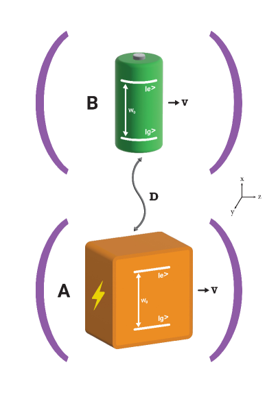
Figure 1: Schematic illustration of a qubit-based open QB composed of a qubit-battery and a qubit-charger moving along the z-axis of two distinct but identical cavity reservoir. The qubits move with constant speed $v$ and are also coupled to each other through the dipole-dipole interaction.

3 Open Moving-Quantum Battery

The open QB under consideration is composed of an atomic two-qubit system, the qubit $A$ as a charger and the qubit $B$ as a quantum battery, coupled to each other trough the dipole-dipole interaction. The battery and charger qubits coupled locally to two independent zero-temperature cavity reservoirs (see Fig. 1). We assume that each qubit moves along the $z$-axis of its cavity at a constant non-relativistic speed $v$. For simplicity we neglect here any scattering [49] or trapping [50] effects and consider the translational motion of the atom qubits being classically. Under the dipole and rotating wave approximation, the entire system is ruled by Hamiltonian (setting $\hbar=1$)

$$H=H_{0}+H_{int},$$ (7)

with

$$H_{0}=H_{A}+H_{B}+H_{R_{A}}+H_{R_{B}}=\sum_{j=A,B}\left(\frac{\omega_{0}}{2}\sigma_{z}^{j}+\sum_{k}\omega_{k}^{j}a_{k}^{j{\dagger}}a_{k}^{j}\right),$$

$$H_{int}=H_{A-B}+H_{A-R_{A}}+H_{B-R_{B}}=D\left(\sigma_{+}^{A}\sigma_{-}^{B}+\sigma_{-}^{A}\sigma_{+}^{B}\right)+\sum_{j=A,B}\sum_{k}f_{k}^{j}(z)\left(\mathfrak{g}_{k}^{j}\sigma_{+}^{j}a^{j}_{k}+H.c.\right).$$ (8)

Here, H.c. stands for Hermitian conjugate, $\sigma_{z}^{j}$, $\sigma_{+}^{j}$, and $\sigma_{-}^{j}$ $(j=A,B)$ are, respectively, the population inversion, raising and lowering operators of the $j$th qubit with transition frequency $\omega_{0}$. $a_{k}^{j\dagger}$ and $a^{j}_{k}$ are, respectively, the creation and annihilation operators of the $k$th mode of the cavity reservoir $j$ with the frequency $\omega_{k}^{j}$. Also, $D$ is coupling constant of the dipole-dipole interaction between the battery and charger qubits, and $\mathfrak{g}_{k}^{j}$ is the coupling constant between the $j$th qubit and $k$th mode of in the cavity reservoir $j$. The effect of translation motion of the battery and charger qubits has been included in the model by introducing the $z$-dependent shape function $f_{k}^{j}(z)$ in the Hamiltonian $H_{int}$. When the battery and charger qubits are moving with same constant velocity $v$, the shape function $f_{k}^{j}(z=vt)$ can be taken into account as

$$f_{k}^{j}(z)=\sin[\omega_{k}^{j}(\beta t-\Gamma)],\qquad\qquad j=A,B$$ (9)

where, $\Gamma=L/c$ with $L$ being the size of the cavity. Also, $\beta=v/c$ where $c$ refers to the speed of light in the vacuum space. This particular form of the shape function can be obtained by imposing an appropriate boundary condition on the cavity reservoirs [51, 39]. Here we describe the translational motion of both battery and charger qubits by classical mechanics ($z=vt$). To this end, we will choose the values of the parameters in such a way that the de Broglie wavelength of qubit $\lambda_{B}$ is significantly smaller than the wavelength $\lambda_{0}$ associated with the resonant transition $\omega_{0}=\omega_{n}$ ($\omega_{n}$ is the central frequency of the cavity field mode) [52, 53]. Furthermore, we consider a situation in which the photon momentum is relatively small than the atomic momentum and thus we neglect the atomic recoil caused by the interaction with the electric field [54]. In the optical regime, to ignore the atomic recoil and consider the translational motion of atoms as classical, the velocity of qubits should be $v\gg 10^{-3}$ [39].

In the interaction picture (IP) generated by the unitary transformation $U=e^{-iH_{0}t}$, the Hamiltonian (3) can be written as follows

$$H_{IP}=D\left(\sigma_{+}^{A}\sigma_{-}^{B}+\sigma_{-}^{A}\sigma_{+}^{B}\right)+\sum_{j=A,B}\sum_{k}f_{k}^{j}(z)\left(\mathfrak{g}_{k}^{j}\sigma_{+}^{j}a_{k}^{j}e^{i(\omega_{0}-\omega_{k}^{j})t}+\mathfrak{g}_{k}^{j\ast}\sigma_{-}^{j}a_{k}^{j{\dagger}}e^{-i(\omega_{0}-\omega_{k}^{j})t}\right).$$ (10)

It is straightforward to show that the total excitation operator $\hat{\mathcal{N}}=\sum_{j=A,B}\left(\sum_{k}\hat{a_{k}}^{j\dagger}\hat{a_{k}}^{j}+\frac{1}{2}\hat{\sigma}_{z}^{j}\right)+1$, commutes with the total Hamiltonian, i.e. $[H,\hat{\mathcal{N}}]=0$ and therefor it is the constant of the motion. This allows us to decompose Hilbert space of the entire qubit-cavity system, $\mathcal{H}=\mathcal{H}_{q}\otimes\mathcal{H}_{R}$ spanned by the basis $\{\left|i_{A},j_{B}\right\rangle\otimes\left|n_{1},n_{2},...,n_{k},...\right\rangle_{R_{A}}|_{n_{1},n_{2},...=0}^{\infty}\otimes\left|m_{1},m_{2},...,m_{k},...\right\rangle_{R_{B}}|_{m_{1},m_{2},...=0}^{\infty}\}$ $\left(i,j=e,g\right)$ into the excitation subspaces, as follows

$$\mathcal{H}=\oplus_{n=0}^{\infty}\mathcal{H}_{n}.$$ (11)

As a result of this decomposition, the dynamics of the entire qubit-reservoir system can be restricted to the excitation subspaces labeled by the total excitation number $n$. Here we are interested to explore dynamics of the entire system in the single-excitation subspace $\mathcal{H}_{1}$ spanned by vectors $\{\left|g_{A},g_{B}\right\rangle\otimes\left|1_{k}\right\rangle_{R_{A}}\left|0_{k}\right\rangle_{R_{B}}|_{k=0}^{\infty},\left|g_{A},g_{B}\right\rangle\otimes\left|0_{k}\right\rangle_{R_{A}}\left|1_{k}\right\rangle_{R_{B}}|_{k=0}^{\infty},\left|e_{A},g_{B}\right\rangle\otimes\left|0_{k}\right\rangle_{R_{A}}\left|0_{k}\right\rangle_{R_{B}},\left|g_{A},e_{B}\right\rangle\otimes\left|0_{k}\right\rangle_{R_{A}}\left|0_{k}\right\rangle_{R_{B}}\}$ in which the single excitation is either in one of the qubits or in the k-th mode of one of cavity reservoirs. We consider a normalized initial state of entire qubit-reservoir as a superposition of $\left|e_{A},g_{B}\right\rangle\left|0_{k}\right\rangle_{R_{A}}\left|0_{k}\right\rangle_{R_{B}}$ and $\left|g_{A},e_{B}\right\rangle\left|0_{k}\right\rangle_{R_{A}}\left|0_{k}\right\rangle_{R_{B}}$ states with the following form

$$|\Psi(0)\rangle=\big{[}c_{1}(0)|e_{A},g_{B}\rangle+c_{2}(0)|g_{A},e_{B}\rangle\big{]}\otimes|0\rangle_{R_{A}}|0\rangle_{R_{B}}.$$ (12)

For times $t>0$, we expand the state vector $|\Psi(t)\rangle$ in terms of the vector basis of the single-excitation subspace $\mathcal{H}_{1}$ as

$$\left|\Psi(t)\right\rangle=\big{[}c_{1}(t)\left|e_{A},g_{B}\right\rangle+c_{2}(t)\left|g_{A},e_{B}\right\rangle\big{]}\otimes\left|0_{k}\right\rangle_{R_{A}}\left|0_{k}\right\rangle_{R_{B}}$$

$$+\left|g_{A},g_{B}\right\rangle\otimes\sum_{k}\big{[}d_{k}(t)\left|1_{k}\right\rangle_{R_{A}}\left|0_{k}\right\rangle_{R_{B}}+d_{k}^{\prime}(t)\left|0_{k}\right\rangle_{R_{A}}\left|1_{k}\right\rangle_{R_{B}}\big{]},$$ (13)

where the time-dependent amplitudes satisfy the normalization requirement

$$\sum_{i=1}^{2}|c_{i}(t)|^{2}+\sum_{k}(|d_{k}(t)|^{2}+|d_{k}^{\prime}(t)|^{2})=1.$$ (14)

By taking the partial traces over the field modes and subsystem A (B), the reduced time-dependent density operator for the battery (charger) in the $\{\left|e\right\rangle,\left|g\right\rangle\}$ basis is obtained as

$$\rho_{A}(t)=|c_{1}(t)|^{2}\left|e_{A}\right\rangle\left\langle e_{A}\right|-\left(1-|c_{1}(t)|^{2}\right)\left|g_{A}\right\rangle\left\langle g_{A}\right|,$$ (15a)

$$\rho_{B}(t)=|c_{2}(t)|^{2}\left|e_{B}\right\rangle\left\langle e_{B}\right|-\left(1-|c_{2}(t)|^{2}\right)\left|g_{B}\right\rangle\left\langle g_{B}\right|.$$ (15b)

Inserting Eq. (3) into the time dependent Schrödinger equation $H_{IP}|\Psi(t)\rangle=i\frac{d}{dt}|\Psi(t)\rangle$, with $H_{IP}$ given in (10), leads to the following set of differential equations for time-dependent amplitudes

$$i\dot{c_{1}}(t)=Dc_{2}(t)+\sum_{k}\mathfrak{g}_{k}^{A}f_{k}^{A}(z)d_{k}(t)e^{i(\omega_{0}-\omega_{k}^{A})},$$ (16a)

$$i\dot{c_{2}}(t)=Dc_{1}(t)+\sum_{k}\mathfrak{g}_{k}^{B}f_{k}^{B}(z)d_{k}^{\prime}(t)e^{i(\omega_{0}-\omega_{k}^{B})},$$ (16b)

$$i\dot{d}_{k}(t)=\mathfrak{g}_{k}^{A\ast}f_{k}^{A}(z)c_{1}(t)e^{-i(\omega_{0}-\omega_{k}^{A})t},$$ (16c)

$$i\dot{d}_{k}^{\prime}(t)=\mathfrak{g}_{k}^{B\ast}f_{k}^{B}(z)c_{2}(t)e^{-i(\omega_{0}-\omega_{k}^{B})t}.$$ (16d)

By integrating Eqs. (16c) and (16d) with the initial condition $d_{k}(0)=0$ and $d_{k}^{\prime}(0)=0$ and putting their solutions, respectively, in Eqs. (16a) and (16b), we get the following integro-differential equations for the amplitudes $c_{1}(t)$ and $c_{2}(t)$

$$\dot{c_{1}}(t)=-iDc_{2}(t)+\int_{0}^{t}F_{A}(t-t^{\prime})c_{1}(t^{\prime})dt^{\prime},$$ (17a)

$$\dot{c_{2}}(t)=-iDc_{1}(t)+\int_{0}^{t}F_{B}(t-t^{\prime})c_{2}(t^{\prime})dt^{\prime},$$ (17b)

where

$$F_{A}(t-t^{\prime})=\sum_{k}|\mathfrak{g}_{k}^{A}|^{2}e^{i(\omega_{0}-\omega_{k}^{A})(t-t^{\prime})}\sin[\omega_{k}^{A}(\beta^{A}t-\Gamma)]\sin[\omega_{k}^{A}(\beta^{A}t^{\prime}-\Gamma)],$$ (18a)

$$F_{B}(t-t^{\prime})=\sum_{k}|\mathfrak{g}_{k}^{B}|^{2}e^{i(\omega_{0}-\omega_{k}^{B})(t-t^{\prime})}\sin[\omega_{k}^{B}(\beta^{B}t-\Gamma)]\sin[\omega_{k}^{B}(\beta^{B}t^{\prime}-\Gamma)],$$ (18b)

are the memory correlation function of the reservoirs $A$ and $B$, respectively. For simplicity, we suppose $F_{A}(t-t^{\prime})=F_{B}(t-t^{\prime})=F(t-t^{\prime})$. In the limit of a large number of modes ( in the continuum limit ), the correlation function $F(t-t^{\prime})$ takes the following form

$$F(t-t^{\prime})=\int d\omega J(\omega)e^{i(\omega_{0}-\omega)(t-t^{\prime})}\sin[\omega(\beta t-\Gamma)]\sin[\omega(\beta t^{\prime}-\Gamma)],$$ (19)

in which $J(\omega)$ is the spectral density of the cavity reservoirs and has the Lorentzian form [51, 55]

$$J(\omega)=\frac{1}{2\pi}\frac{\gamma\lambda^{2}}{(\omega_{0}-\omega-\Delta)^{2}+\lambda^{2}},$$ (20)

where $\lambda$ defines the spectral width of the coupling which is connected to the memory time $\tau_{E}$ by the relation $\tau_{E}=\lambda^{-1}$ and $\gamma$ refers to the qubit-environment coupling strength which is related to the relaxation time scale $\tau_{R}$ by $\tau_{R}\approx\gamma^{-1}$. Also $\Delta$ is the detuning of $\omega_{0}$ and the central frequency of the cavity. The weak and strong coupling regimes can be distinguished by comparing $\tau_{E}$ and $\tau_{R}$, in other words with an increasing $\frac{\tau_{E}}{\tau_{R}}=\frac{\gamma}{\lambda}$ ratio, the interaction will transition into a strong coupling or a non-Markovian regime [55].
By inserting the Eq. (20) into the Eq. (19) and after some calculations, in the continuum limit ($\Gamma\rightarrow\infty$), the correlation function is simplified as

$$F(t-t^{\prime})=\frac{\gamma\lambda}{4}\cosh[\beta\overline{\lambda}(t-t^{\prime})]e^{-(\lambda-i\Delta)|t-t^{\prime}|}$$ (21)

with $\overline{\lambda}=\lambda+i(\omega_{0}-\Delta)$.
In view of (21), taking the Laplace transformations of both sides of the differential Eqs. (17a) and (17b) and using the convolution property $\mathcal{L}[\int_{0}^{t}\mathbf{A}(t-t^{\prime})\mathbf{B}(t^{\prime})dt^{\prime}]=\mathbf{A}(s)\mathbf{B}(s)$ yields

$$sc_{1}(s)-c_{1}(0)=-iDc_{2}(s)-F(s)c_{1}(s),$$ (22a)

$$sc_{2}(s)-c_{2}(0)=-iDc_{1}(s)-F(s)c_{2}(s),$$ (22b)

where the functions $c_{1}(s)$ and $c_{2}(s)$ are the Laplace transformations of the $c_{1}(t)$ and $c_{2}(t)$, respectively, and $F(s)$ is the Laplace transforms of $F(t-t^{\prime})$ which has the following explicit form

$$F(s)=\frac{\gamma\lambda}{4}\frac{s+\overline{\lambda}}{(s+\overline{\lambda})^{2}-\beta^{2}\overline{\lambda}\,^{2}}.$$ (23)

By reformulating the Eqs. (22a) and (22b), we get a general solution for $c_{1}(s)$ and $c_{2}(s)$ as follows

$$c_{1}(s)=\frac{s+F(s)}{\big{(}s+F(s)\big{)}^{2}+D^{2}}c_{1}(0)-i\frac{D}{(s+F(s))^{2}+D^{2}}c_{2}(0),$$ (24a)

$$c_{2}(s)=\frac{s+F(s)}{\big{(}s+F(s)\big{)}^{2}+D^{2}}c_{2}(0)-i\frac{D}{(s+F(s))^{2}+D^{2}}c_{1}(0).$$ (24b)

In continuation, by applying the inverse Laplace transformation on the both side of the above equations, we obtain finally $c_{1}(t)$ and $c_{2}(t)$, as

$$c_{1}(t)=\frac{1}{2}\bigg{(}c_{1}(0)\Re(\mathcal{M}(t))-ic_{2}(0)\Im(\mathcal{M}(t))\bigg{)},$$ (25a)

$$c_{2}(t)=\frac{1}{2}\bigg{(}c_{2}(0)\Re(\mathcal{M}(t))-ic_{1}(0)\Im(\mathcal{M}(t))\bigg{)},$$ (25b)

where, $\Re(x)$ ($\Im(x)$) is real (imaginary) part of $x$, and

$$\mathcal{M}(t)=\sum_{i,j,k=1}^{3}\varepsilon_{ijk}\frac{e^{q_{i}t}(q_{j}-q_{k})\bigg{(}(q_{i}+\overline{\lambda})^{2}-\beta^{2}\overline{\lambda}^{2}\bigg{)}}{\prod_{i=1}^{3}\prod_{j=i+1}^{3}(q_{i}-q_{j})},$$ (26)

with $\varepsilon_{ijk}$ is the Levi-Civita symbol and $q_{i}(i=1,2,3)$ are the roots of

$$q^{3}+q^{2}(2\overline{\lambda}-i\text{D})+q\left(\frac{\gamma\lambda}{4}+\overline{\lambda}(\overline{\lambda}-2i\text{D})-\beta^{2}\overline{\lambda}^{2}\right)+\frac{\gamma\lambda\overline{\lambda}}{4}+i\text{D}\overline{\lambda}^{2}\left(\beta^{2}-1\right)=0.$$ (27)

With substitution (25a) and (25b), respectively, into the reduced density matrices (15b) and (15a), and then using the $\Delta E_{A(B)}=\texttt{Tr}\{\rho_{A(B)}(t)H_{A(B)}\}-\texttt{Tr}\{\rho_{A(B)}(0)H_{A(B)}\}$ , the internal energy of the charger and battery are deduced as

$$\Delta E_{A}=\omega_{0}\left(|c_{1}(t)|^{2}-|c_{1}(0)|^{2}\right),\quad\quad\Delta E_{B}=\omega_{0}\left(|c_{2}(t)|^{2}-|c_{2}(0)|^{2}\right).$$ (28)

On the other hand, one can obtain ergotropy of the battery by substitution Eq. (15b) with Eq. (4). So, we have

$$W_{B}=\omega_{0}\left(2|c_{2}(t)|^{2}-1\right)\Theta\left(|c_{2}(t)|^{2}-\frac{1}{2}\right),$$ (29)

where $\Theta(x-x_{0})$ is the Heaviside function, which satisfies $\Theta(x-x_{0})=0$ for $x<x_{0}$, $\Theta(x-x_{0})=\frac{1}{2}$ for $x=x_{0}$ and $\Theta(x-x_{0})=1$ for $x>x_{0}$.

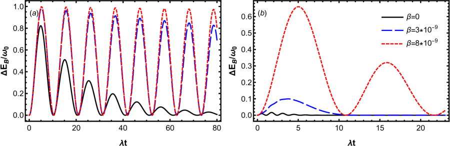
Figure 2: Dynamics of the stored energy $\Delta E_{B}(t)$ for the different values of $\beta$ by setting $\omega_{0}=1.5\times 10^{9}\lambda$, $D=0.3\lambda$ and $\Delta=0.3\lambda$. The panels (a) displays the Markovian dynamics with $\gamma=0.1\lambda$, while the panels (b) displays the non-Markovian dynamic with $\gamma=20\lambda$.

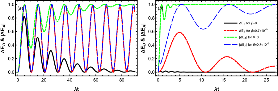
Figure 3: Dynamics of the stored energy $\Delta E_{B}$ and internal energy of charger $|\Delta E_{A}|$ for the different values of $\beta$ by setting $\omega_{0}=1.5\times 10^{9}\lambda$, $D=0.3\lambda$ and $\Delta=0$. The panels (a) displays the Markovian dynamics with $\gamma=0.1\lambda$, while the panels (b) displays the non-Markovian dynamic with $\gamma=20\lambda$.

4 Numerical Results and Discussion

In this section, we will analyze the charging dynamics of the introduced open moving-battery in the weak and strong coupling regimes. In particular, we explore the role of the movement of QB on the dynamical behavior of performance indicators including stored energy, ergotropy and efficiency. In our following analysis, we choose the optical regime parameters [56, 57] and consider that qubit transition frequency as $\omega_{0}=1.5\times 10^{9}\lambda$. In what follows, we consider an initial condition in which the battery is initially empty and the charger has the maximum energy, i.e. $c_{1}(0)=0$, $c_{2}(0)=1$.

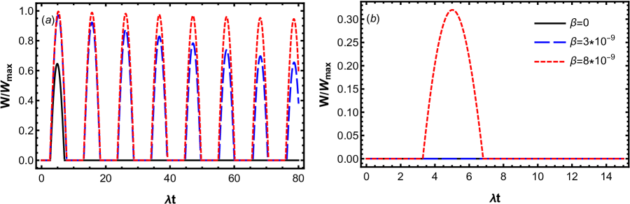
Figure 4: Dynamics of ergotropy $W_{B}$ for the different values of $\beta$ by setting $\omega_{0}=1.5\times 10^{9}\lambda$, $D=0.3\lambda$ and $\Delta=0$. The panels (a) displays the Markovian dynamics with $\gamma=0.1\lambda$, while the panels (b) displays the non-Markovian dynamic with $\gamma=20\lambda$.

In Fig. 2, we plot the Markovian and non-Markovian dynamics of the stored energy $\Delta E_{B}$ for the initial state $\left|\Psi(0)\right\rangle=\left|g\right\rangle_{A}\left|e\right\rangle_{B}\otimes\left|0\right\rangle_{R_{B}}\left|0\right\rangle_{R_{B}}$, by considering different values of the QB speed $\beta$. In panel (a), the battery is charged in the Markovian dynamics with $(\gamma=0.1\lambda)$, while in panel (b), it is charged in a non-Markovian dynamics with $(\gamma=20\lambda)$. Here we consider a situation at which the charger and battery’s qubits are both in resonance with the reservoir modes by setting $\Delta=0$. According to this figure, the positive impact of the translational motion of the charger and batter’s qubits in controlling the stored energy of battery is clearly visible in both Markovian and non-Markovian charging processes. As can be seen in both Figs. 2(a) and (b), when the charger and battery’s qubits are at rest inside their cavity reservoirs, the stored energy in the battery $\Delta E_{B}$ decays into zero at sufficiently long times. However the rate of these decays decreases regularly by gradual growth of the qubit velocity, and therefore the energy stored in the battery and consequently the charging process is strongly protected from the environmental noises. Comparing Fig. 2(a) with Fig. 2(b) clearly reveals a fundamental difference between Markovian and non-Markovian charging processes. The maximal amount of stored energy in the Markovian charging process is more than those of the non-Markovian charging process. The reason stems from the nature of the qubit-cavity coupling. In the non-Markovian charging process, the coupling strength of charger’s qubit to the cavity modes is greater than its coupling to the battery’s qubit, therefore, the initial internal energy of charger has more tendency to evolve toward the reservoir than to the battery. Moreover, since the motional effect of QB has been included in battery-cavity and charger-cavity coupling strength, it seems that increasing speed of QB decreases the charger-cavity coupling strength in favor of to charger-battery coupling strength, which increases the energy stored in the battery.

In order to get more insight to this area and a deeper understanding of the relationship between the charger and battery energy, in Fig. 2 we have illustrated the energy stored in the battery at the end of charging process as well as the energy that the charger loses at the same time. Here $\Delta E_{B}$ and $|\Delta E_{A}|$ have been plotted as a function of the dimensionless time $\lambda t$ for the qubit velocities $\beta=0$ and $\beta=0.7\times 10^{-9}$ in the Markovian and non-Markovian regimes. In the non-Markovian charging process, $|\Delta E_{A}|$ is much more than $\Delta E_{B}$ for a given $\beta$ as shown in Fig. 3(b). This implies that the internal energy of the charger is not completely transferred to the battery. Fig. 3(b) also shows that, when the charger and battery’s qubits are at rest inside their cavity reservoirs, the charger’s qubit immediately loses a large amount of its initial energy without being transferred to the battery. However, increasing the qubit velocity (decreasing the ratio of charger-cavity coupling strength to charger-battery coupling strength) during the non-Markovian process, decreases the initial loss-rate of the charger, and therefore improves the energy transfer in the charging processes.

The relationship between the charger and battery energy in the Markovian charging process is drastically different from that in the non-Markovian charging process. One can infer from Fig. 3(a) that, for the static battery-charger system ($\beta=0$), the total energy of the charger can be transferred to the battery in the Markovian short-charging process, where we have $|\Delta E_{A}|=\Delta E_{B}$. Interestingly, when the qubits move with the velocity $\beta=0.7\times 10^{-9}$, $|\Delta E_{A}|=\Delta E_{B}$ holds at any charging time. So, we conclude again that a robust Markovian charging against the arisen dissipation can be achieved, when the qubits move with higher velocities.

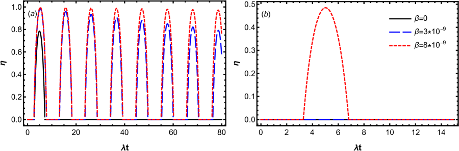
Figure 5: Dynamics of efficiency $\eta(t)$ for the different values of $\beta$ by setting $\omega_{0}=1.5\times 10^{9}\lambda$, $D=0.3\lambda$ and $\Delta=0$. The panels (a) displays the Markovian dynamics with $\gamma=0.1\lambda$, while the panels (b) displays the non-Markovian dynamic with $\gamma=20\lambda$.

In the following, we examine the influence of translational motion of the battery-charger system on the dynamics of ergotropy. In Fig. 4, we plot $W/W_{max}$ as a function of $\lambda t$ for the different values of $\beta$ in the Markovian (Fig. 4(a)) and non-Markovian (Fig. 4(b)) regimes. Our numerical results in Fig. 4(a) and (b) illustrate that, the effect of translational motion of QB on the ergotropy is also constructive in both Markovian and non-Markovian regimes. Fig. 4(b) shows that, in the non-Markovian regime, in the cases of stationary ($\beta=0$) and slowly moving ($\beta=3\times 10^{-9}$) qubits, we are not able to extract useful work from the QB, but in this regime a considerable work can be extracted, as the qubits move with a higher velocity ($\beta=0.8\times 10^{-9}$). Our numerical results in Fig. 4(a) illustrate that, the effect of translational motion of QB on the ergotropy is more considerable in the Markovian case. We observe that, in the Markovian regime, increasing the speed of QB $\beta$ (decreasing the qubit-reservoir coupling) not only boosts the ergotropy, but also increases the number of time zones in which work can be extracted. Accordingly, a strong robust charging process can be established in the higher speed limit, in which the extractable work approaches to its maximum value.

Finally, we examine the effect of translational motion of QB on the Markovian and non-Markovian charging efficiency. The results for Markovian and non-Markovian charging processes are presented in Fig. 5(a) and 5(b), respectively. Here we consider the same parameter values as Fig. 4. Comparing Figs. 4 and 3 reveals that both ergotropy and efficiency are positively affected by the translational motion of QB. However the efficiency is influenced more than the ergotropy; the amount of increment in efficiency is more than the ergotropy in both Markovian and non-Markovian charging processes.

5 Outlook and summary

To summarize, we proposed a mechanism for robust charging process of an open qubit-based quantum battery (QB) whose robustness can be well controlled by the translational motion of the charger and battery in both Markovian and non-Markovian dynamical regimes. Both the battery and charger’s qubits move with a same speed inside two separated identical environments, and are directly coupled by the dipole-dipole interaction. We showed that the stored energy, ergotropy and efficiency of the moving QB regularly increased with the gradual growth of the charger and battery speed, thereby improving its charging performance. The constructive role of the translational movement of QB in controlling the charging process arises from the attachment of qubits velocities to the qubit-reservoir coupling strength (see Eq. (3)). According to the adopted charging protocol, a weak qubit-reservoir coupling is required for a strongly robust charging process which can be fulfilled by adjusting $\beta$ to the higher velocities.

Our results represent a further control strategy to have a robust QB with a natural implementation in cavity-QED context. The strategy can be easily implemented also in the circuit-QED setups where the qubit position slowly varies linearly with time and also the qubit-cavity interaction is tuned through a sinusoidal position-dependent coupling [58].

In perspective, we believe that this strategy can be used to control the performance of the discharging of a qubit-based QB to an available consumption hub. Further efforts in this field can be devoted to use the proposed strategy for improving the performance of the two-photon based charging process where the moving-QB is coupled with a cavity reservoir by means of a two-photon relaxation.

Data availability
The datasets used and analysed during the current study available from the corresponding author on reasonable request.

References

- [1] R. Alicki and M. Fannes, Entanglement boost for extractable work from ensembles of quantum batteries, Phys. Rev. E 87, 042123 (2013).
- [2] P. Strasberg, G. Schaller, T. Brandes, and M. Esposito, Quantum and information thermodynamics: A unifying framework based on repeated interactions, Phys. Rev. X 7, 021003 (2016).
- [3] S. Vinjanampathy and J. Anders, Quantum thermodynamics, Cont. Phy. 57, 545 (2016).
- [4] J. Goold, M. Huber, A. Riera, L. del Rio, and P. Skrzypczyk, The role of quantum information in thermodynamics: a topical review, J. Phys. A: Math. Theor. 49, 143001 (2016).
- [5] M. Campisi, P. Hänggi, and P. Talkner, Colloquium: Quantum fluctuation relations: Foundations and applications, Rev. Mod. Phys. 83, 1653 (2011).
- [6] D. Gelbwaser-Klimovsky, W. Niedenzu and G. Kurizki, Thermodynamics of quantum systems under dynamical control, Adv. At. Mol. Opt. Phys., 64, 329 (2015).
- [7] M. Horodecki and J. Oppenheim,Fundamental limitations for quantum and nanoscale thermodynamics, Nature Comm. 4, 2059 (2013).
- [8] D. Farina, G. M. Andolina, A. Mari, M. Polini and V. Giovannetti, powerful charging of quantum batteries, Phys. Rev. B 99, 035421 (2019).
- [9] Y-Y. Zhang, T-R. Yang, L. Fu and X. Wang, Powerful harmonic charging in a quantum battery, Phys. Rev. E 99, 052106 (2019).
- [10] L. Fusco, M. Paternostro, and G. D. Chiara, Work extraction and energy storage in the Dicke model, Phys. Rev. E 94, 052122 (2016).
- [11] R. R. Rodriguez, B. Ahmadi, P. Mazurek, S. Barzanjeh, R. Alicki and P. Horodecki, catalysis in charging quantum batteries, Phys. Rev. A 107, 042419 (2023).
- [12] J. Carrasco, J. R. Maze, C. Hermann-Avigliano and F. Barra, collective enhancement in dissipative quantum batteries, Phys. Rev. E. 105, 064119 (2022).
- [13] M. Gumberidze, M. Kolár and R. filip, Measurement induced Synthesis of coherent Quantum Batteries, Sci. Rep 9, 19628 (2019).
- [14] D. Ferraro, M. Campisi, G. M. Andolina, V. Pellegrini and M. Polini, High-power collective charging of a solid-state quantum battery, Phys. Rev. Lett. 120, 117702 (2018).
- [15] P. Forn-Dílaz, J. J. Garcíla-Ripoll, B. Peropadre, J.-L. Orgiazzi, M. A. Yurtalan, R. Belyansky, C. M. Wilson, and A. Lupascu, Ultrastrong coupling of a single artificial atom to an electromagnetic continuum in the nonperturbative regime, Nat. Phys. 13, 39 (2016).
- [16] Bruzewicz, C.D.; Chiaverini, J.; McConnell, R.; Sage, J.M. Trapped-Ion Quantum Computing: Progress and Challenges. Appl. Phys. Rev. 2019, 6, 021314..
- [17] K. Baumann, C. Guerlin, F. Brennecke, and T. Esslinger, The dicke quantum phase transition with a superfluid gas in an optical cavity, Nature (London) 464, 1301 (2010)
- [18] Devoret, M.H.; Schoelkopf, R. J. Superconducting Circuits for Quantum Information: An Outlook. Science 2013, 339, 1169
- [19] D. Farina, G. M. Andolina, A. Mari, M. Polini, and V. Giovannetti, Charger-mediated energy transfer for quantum batteries: Anopen-system approach. Phys. Rev. B 99, 035421 (2019).
- [20] C. Ou, R. V. Chamberlin and S. Abe, Lindbladian operators, von Neumann entropy and energy conservation in time-dependent quantum open systems, Physica A 466, 450 (2017).
- [21] M. Carrega, A. Crescente, D. Ferraro, and M. Sassetti, Dissipative dynamics of an open quantum battery. New J. Phys. 22, 083085 (2020).
- [22] F. Barra, Dissipative charging of a quantum battery, Phys. Rev. Lett. 122, 210601 (2019).
- [23] A. C. Santos, Quantum advantage of two-level batteries in self-discharging process, Phys. Rev. E 103, 042118 (2021).
- [24] L. P. Garcia-Pintos, A. Hamma, A. del Campo, Fluctuations in extractable work bound the charging power of quantum batteries. Phys. Rev. Lett. 125, 040601 (2020).
- [25] F. H. Kamian, F. T. Tabesh, S. Salimi, F. Kheirandish, and A. C. Santos, Non-markovian effects on charging and selfdischarging processes of quantum batteries, New J. Phys. 22, 083007 (2020).
- [26] F. T. Tabesh, F. H. Kamin, and S. Salimi, Environmentmediated charging process of quantum batteries, Phys. Rev. A 102, 052223 (2020).
- [27] F. Centrone, L. Mancino, M. Paternostro, Charging batteries with quantum squeezing, https://doi.org/10.48550/arXiv.2106.07899.
- [28] J. Q. Quach and W. J. Munro, Using dark states to charge and stabilise open quantum batteries, Phys. Rev. Applied 14, 024092 (2020).
- [29] M. T. Mitchison, J. Goold and J. Prior, Charging a quantum battery with linear feedback control, Quantum 5, 500 (2021).
- [30] Y. Yao and X. Q. Shao, Phys. Rev. E Optimal charging of open spin-chain quantum batteries via homodyne-based feedback control, 106, 014138 (2022).
- [31] S. Borisenok, Ergotropy of quantum battery controlled via target attractor feedback, J. Appl. Phys. 12, 43 (2020).
- [32] R. R. Rodriguez, B. Ahmadi, G. Suarez, P. Mazurek, S. Barzanjeh, P. Horodecki, Optimal quantum control of charging quantum batteries, arXiv:2207.00094 [quant-ph].
- [33] F. Mazzoncini, V. Cavina, G. M. Andolina, P. A. Erdman and V. Giovannetti, Optimal control methods for quantum batteries, Phys. Rev. A 107 (2023) 032218.
- [34] N. Behzadi and H. Kassani, Mechanism of controlling robust and stable charging of open quantum batteries, J. Phys. A: Math. Theor. 55, 425303 (2022).
- [35] J. L. Li, H. Z. Shen and X. X. Yi, Quantum batteries in non-Markovian reservoirs, Opt. Lett 21, 5614 (2022).
- [36] A. C. Santos, B. Çakmak, S. Campbell and N.T. Zinner, Stable adiabatic quantum batteries, Phys. Rev. E 100, 032107 (2019).
- [37] J. Liu, D. Segal, Boosting quantum battery performance by structure engineering, arXiv:2104.06522 [quant-ph].
- [38] J. Taghipour, B. Mojaveri and A. Dehghani, Witnessing entanglement between two two-level atoms coupled to a leaky cavity via two-photon relaxation, Eur. Phys. J. Plus 137, 772 (2022).
- [39] A. Mortezapour, M. A. Borji, and R. L. Franco, Protecting entanglement by adjusting the velocities of moving qubits inside non-Markovian environments, Laser Phys. Lett 14, 055201 (2017).
- [40] W. Chao and F. Mao-Fa, The entanglement of two moving atoms interacting with a single-mode field via a three-photon process, Chin. Phys. B 19, 020309 (2010).
- [41] S. Golkar and M. K. Tavassoly and A. Nourmandipour, Entanglement dynamics of moving qubits in a common environment, J. Opt. Soc. Am. B 37, 400 (2020).
- [42] S. Golkar and M. K. Tavassoly And A. Nourmandipour, Qubit movement-assisted entanglement swapping, Chin. Phys. B. 29, 050304 (2020).
- [43] B. Mojaveri, A. Dehghani and J. Taghipour, Control of entanglement, single excited-state population and memory-assisted entropic uncertainty of two qubits moving in a cavity by using a classical driving field, Eur. Phys. J. Plus 137, 1065 (2022).
- [44] J. Taghipour, B. Mojaveri and A. Dehghani, Witnessing entanglement between two two-level atoms moving inside a leaky cavity under classical control, Mod. Phys. Lett. A 37, 2250141 (2022).
- [45] Q. Wang, R. Liu, H. M. Zou, D. Long and J. Wang, Entanglement dynamics of an open moving-biparticle system driven by classical-field, Phys. Scr. 97, 055101, (2022).
- [46] A. E. Allahverdyan, R. Balian and T. M. Nieuwenhuizen, Maximal work extraction from finite quantum systems. Eur. phys. Lett 67, 565 (2004).
- [47] G. Francica, J. Goold, F. Plastina, and M. Paternostro, Daemonic ergotropy: enhanced work extraction from quantum correlations, npj Quantum Inf. 3, 12 (2017).
- [48] B. Çakmak, Ergotropy from coherences in an open quantum system, Phys. Rev. E 102, 042111 (2020).
- [49] B.G. Englert, J. Schwinger, A.O. Barut and M.O. Scully, Reflecting slow atoms from a micromaser field, Eur. Phys. Lett 14, 25 (1991).
- [50] S. Haroche, M. Brune and J.M. Raimond, Trapping atoms by the vacuum field in a cavity, Eur. Phys. Lett 14, 19 (1991).
- [51] C. Leonardi and A. Vagliea, Non-markovian dynamics and spectrum of a moving atom strongly coupled to the field in a damped cavity, Opt. Commun 97, 130 (1993).
- [52] F. Nosrati, A. Mortezapour and R. Lo Franco, Validating and controlling quantum enhancement against noise by the motion of a qubit, Phys. Rev. A. 101, 012331 (2020).
- [53] R. J. Cook, Atomic motion in resonant radiation: An application of Ehrenfest’s theorem, Phys. Rev. A. 20, 224 (1979).
- [54] M. Wilkens, Z. Bialynicka-Birula and P. Meystre, Spontaneous emission in a Fabry-Pérot cavity: The effects of atomic motion, Phys. Rev. A. 45, 477 (1992).
- [55] H. P. Breuer and F. Petruccione, The Theory of Open Quantum Systems (Oxford University Press, Oxford, New York, 2002).
- [56] C. J. Hood et al., The Atom-Cavity Microscope: Single Atoms Bound in Orbit by Single Photons, Science 287, 1447 (2000).
- [57] P. W. H. Pinkse et al., Trapping an atom with single photons, Nature 404, 365 (2000).
- [58] P. J. Jones, J. A. M. Huhtamäki, K. Y. Tan and M. Möttönen, Tunable electromagnetic environment for superconducting quantum bits, Sci. Rep. 3, 1987 (2013).