RGB-D-Fusion: Image Conditioned Depth Diffusion of Humanoid Subjects

Abstract

We present RGB-D-Fusion, a multi-modal conditional denoising diffusion probabilistic model to generate high resolution depth maps from low-resolution monocular RGB images of humanoid subjects. RGB-D-Fusion first generates a low-resolution depth map using an image conditioned denoising diffusion probabilistic model and then upsamples the depth map using a second denoising diffusion probabilistic model conditioned on a low-resolution RGB-D image. We further introduce a novel augmentation technique, depth noise augmentation, to increase the robustness of our super-resolution model.

I Introduction

From immersive communications, games, virtual production, to virtual try-on and virtual fitting rooms, having an accurate 3D presentation of the body of a person is fundamental. For this, one would typically need to use a professional 3D capture stage with many cameras pointing at the person in the center of the stage, and then put all the videos together using a 3D reconstruction algorithm, such as the ones proposed by Guo et al. (2019), Collet et al. (2015) or Pagés et al. (2018). These setups are complex (huge amount of data to manage, complicated calibration processes, high processing times) and expensive (a high number of cameras, professional lighting, computers, GPUs, networks and more), so to overcome these challenges, modern deep learning techniques aim to simplify the capture process by replacing the multi-camera setup with a single camera, from a single viewpoint. For example, Saito et al. (2019), Saito et al. (2020), and Xiu et al. (2022) generate a full body 3D model of a person, Escribano et al. (2022) propose a way to generate the textures of occluded areas. However, all these techniques output relatively low-resolution considering the target application, and they struggle with complicated poses where depth is difficult to convey from a single viewpoint.

To overcome these challenges, some approaches include additional information into the capturing process, including depth, which typically comes from a consumer-level depth sensor. Although new generation consumer-level depth sensors have significantly improved during the last few years, they still present high levels of noise and sometimes fail to capture details when the subjects are at a distance where their body can be fully captured (at around 2m and farther), and they are still sensitive to sun light (which interferes with the infra-red light these sensors typically use), dark materials (which absorb infra-red light) and non-Lambertian surfaces.

In this work, we propose a new approach to generate high-resolution depth maps of humans using a single low-resolution image as input, using denoising diffusion probabilistic models (DDPMs). Our multi-modal DDPM was trained using high-resolution depth maps, extracted from a large dataset of photorealistic 3D models captured by Volograms (Pagés et al., 2021), which allows us to obtain depth maps with higher accuracy than consumer-level depth sensors.

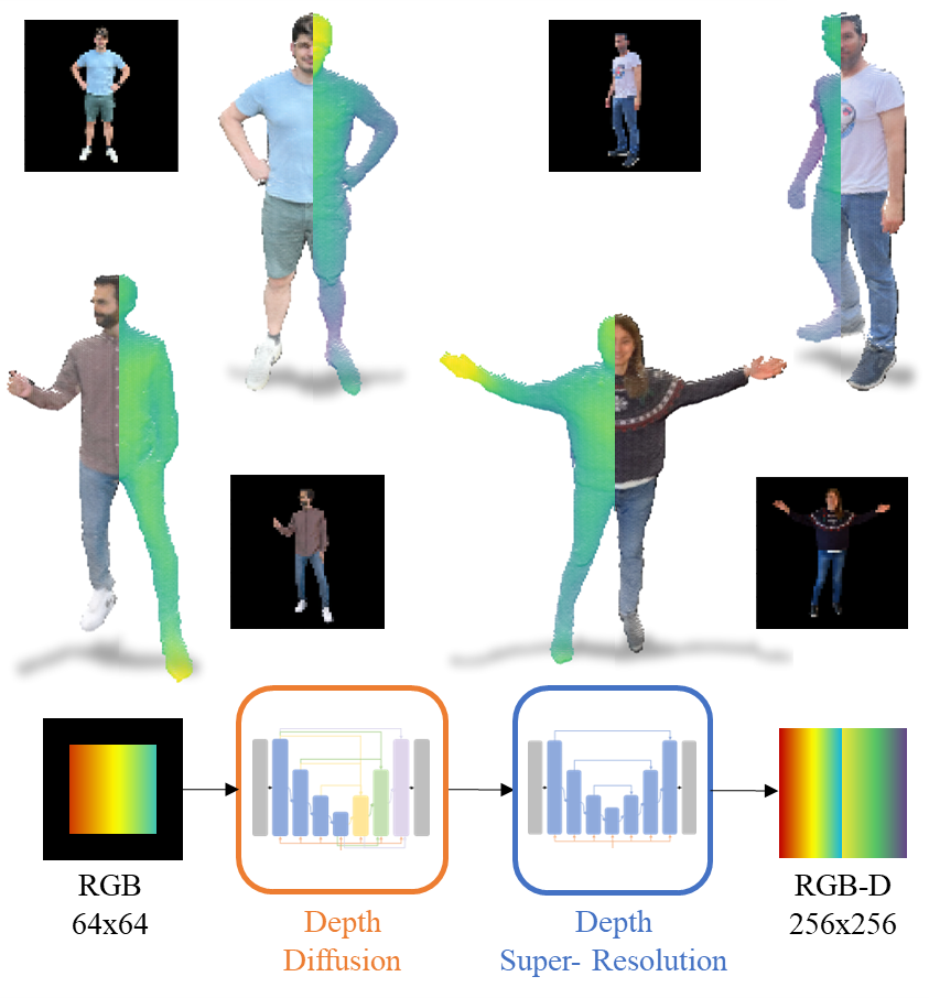
Figure 1: Our RGB-D-Fusion framework generates a high-resolution RGB-D image from a low-resolution RGB image of humanoid subjects. First, a low resolution depth map is generated using a conditional DDPM. Then, the depth is upsampled to a higher resolution using a second DDPM.

Following the taxonomy for multi-modal deep learning systems by Zhan et al. (2022) we frame RGB-D-Fusion as a multi-modal generative translation task using a joint data representation of our input modalities RGB and depth. No alignment is performed between these modalities since our data is perfectly aligned during generation. We further perform parallel data co-learning since our RGB and depth pairs inherently share a direct correspondence between their instances.

We summarize our main contributions of this paper as follows:

1. We provide a framework for high resolution dense monocular depth estimation using diffusion models.

2. We perform super-resolution for dense depth data conditioned on a multi-modal RGB-D input condition using diffusion models.

3. We introduce a novel augmentation technique, namely depth noise, to enhance the robustness of the depth super-resolution model.

4. We perform rigorous ablations and experiments to validate our design choices.

II Related Work

In this section, we situate our work within a broader context and offer a concise summary of other relevant studies.

II-A Denoising Diffusion Probabilistic Models

Denoising diffusion models are a type of generative deep learning models first formulated by Sohl-Dickstein et al. (2015) and further extended to Denoising Diffusion Probabilistic models (DDPMs) by Ho et al. (2020); Nichol and Dhariwal (2021). These models use a Markov Chain to gradually convert one simple and well-known distribution (e.g. a Gaussian distribution) into a usually more complex data distribution the model can sample from.

Diffusion models have been applied to many applications and modalities including image generation (Dhariwal and Nichol, 2021), image-to-image translation (Saharia et al., 2022a), super-resolution (Ho et al., 2021; Saharia et al., 2021), video (Ho et al., 2022; Harvey et al., 2022; Yang et al., 2022), audio (Kong et al., 2021; Lee et al., 2022), text-to-image (Ramesh et al., 2022; Nichol et al., 2022a; Saharia et al., 2022b), and simultaneous multi-modal generation (Ruan et al., 2023).

In the generative learning trilemma formulated by Xiao et al. (2022), which states that generative models cannot satisfy all three key requirements fast sampling, high quality samples and mode coverage, diffusion models have shown good results in high quality image generation (Rampas et al., 2023; Ho et al., 2021) and mode coverage. While Variational Auto-Encoders (VAEs) (Kingma and Welling, 2022; Razavi et al., 2019) and flow based models (Dinh et al., 2017; Durkan et al., 2019) are strong in covering multi-modal data distributions and can be sampled from very fast, the quality of their samples is usually not as high as of Generative Adversarial Models (GANs) or diffusion models. GANs (Goodfellow et al., 2014; Brock et al., 2019; Kirch et al., 2022) on the other-hand produce high quality images and are sampled quickly but are prone to mode collapse and often do not cover the entire data distribution.

DDPMs require many reverse diffusion steps (often several hundreds or even thousands of steps) to sample from, making it difficult train and deploy them even on modern GPUs. Hence it is no surprise that a lot of research focuses on increasing the sample speed of diffusion models by reducing the number of required steps (Song et al., 2022; Xiao et al., 2022; Nichol and Dhariwal, 2021; Salimans and Ho, 2022; Chung et al., 2022), perform diffusion in the latent space rather than the full-resolution data distribution (Preechakul et al., 2022; Rombach et al., 2022; Sinha et al., 2021; Gu et al., 2022; Tang et al., 2023) or formulate the diffusion problem as time-continuous problem to take advantage of accelerated stochastic differential equations (SDE) solvers (Song et al., 2021b, a; Song and Ermon, 2020; Karras et al., 2022).

To control the output of the model it must be provided with an additional condition input. The model might be conditioned on another input of the same modality like in colorization (Saharia et al., 2022a), inpaintings (Batzolis et al., 2021), generation from semantic mask (Meng et al., 2022) or image super-resolution (Saharia et al., 2021; Ho et al., 2021), on an input of different modality like in depth estimation (Duan et al., 2023) or segmentation (Baranchuk et al., 2022), on class labels (Dhariwal and Nichol, 2021) or on text prompts (Ramesh et al., 2022; Nichol et al., 2022a; Saharia et al., 2022b); to name a few.

Depending on the representation of the condition input, it might be concatenated with the noise input (Batzolis et al., 2021), fed to multiple layers within the network like adaptive instance normalization (Karras et al., 2019) or via an independent network branch (Zhang and Agrawala, 2023). Beside the architectural choice one must also decide how strong the condition should be. One could only apply it for certain time steps in the reverse diffusion process, only apply it during inference on an unconditionally trained model (Choi et al., 2021) or using guidance, which applies a weighted sum of a conditional and unconditional generation and hence trades-off sample diversity with sample quality. Among others, guidance can be performed with an additionally trained classifier (Nichol and Dhariwal, 2021), by training the diffusion model conditionally and unconditionally at the same time and sampling using a weighted sum of both (Ho and Salimans, 2022) or by using pre-trained CLIP embeddings (Nichol et al., 2022a; Ramesh et al., 2022).

II-B Monocular Depth Estimation

Knowledge on the depth of a scene is crucial in a vast number of applications including virtual reality (VR), augmented reality (AR), environment perception, autonomous driving, robotics, state estimation, navigation, mapping and many more. Various surveys (Bhoi, 2019; Zhao et al., 2020; Ming et al., 2021; Masoumian et al., 2022) summarize the rich and extensive literature on monocular depth estimation; the estimation of the depth based on a single image; an inherently ill-posed and ambiguous problem.

In contrast, conventional geometric-based approaches such as structure from motion and stereo vision matching rely on geometric constraints and multiple viewpoints to reconstruct 3D structures. On the other hand, sensor-based methods leverage dedicated hardware like LiDAR sensors or RGB-D cameras to directly capture depth information. While these methods find practical application, they suffer from significant limitations including high hardware expenses, imprecise and sparse predictions, and limited accessibility for consumer use.

Many different representations can be deployed to obtain depth information: 2D depth maps (dense or sparse), 3D point cloud, 3D pseudo point cloud predicted from other modality (e.g. stereo camera), camera independent disparity maps, light fields, neural radiance fields (NERFs, Mildenhall et al. (2021)), 3D meshes, voxels and height maps to name a few.

Numerous deep learning based approaches for monocular depth estimation have been researched in recent years. Lu et al. (2022), Chen et al. (2018) and Zhang et al. (2020) train their models using stereo images while inferring only single view images. The model either learns the correspondence between the two views and can reconstruct the other view or the model incorporates the knowledge of a stereo camera into its weights and hence strengthen its capability to extract meaningful features from a single image. Yue et al. (2022) and Zhao et al. (2022) apply a multi-task training objective by not only predicting depth but also other related tasks (e.g. normal vector prediction) that help the model to learn a more profound representation and understanding of the scene which also benefits the downstream task of depth estimation. Watson et al. (2021) and Bian et al. (2021) use mono camera videos to estimate the depth.

Other deep learning-based approaches focus on multiple sensor modalities to estimate the depth of the scene. Zhang et al. (2022) use LiDAR point clouds in combination with stereo images, Eldesokey et al. (2020) use monocular RGB images combined with sparse LiDAR point clouds, Liu et al. (2020) input monocular RGB combined with a depth map and Piao et al. (2021) combine a single RGB image with a focal stack.

In this work, we focus on monocular depth estimation using single RGB images as input and generating dense depth maps as output. We observed that most model architectures are based on GANs, VAEs or similar approaches. We hence further review the usage of diffusion models in the field of depth estimation.

II-C Depth Diffusion

We observe that very little work has been published on monocular depth estimation using diffusion models. We hypothesize that one of the major reasons is the necessity for fast sampling constraint by real-time applications like autonomous driving. We are certain that the community will find a way to further increase the sampling speed in a future and hence we see great potential in diffusion models for monocular depth estimation.

Saxena et al. (2023) used a diffusion model to perform monocular depth estimation on indoor and outdoor scenes introducing a preprocessing step to complete incomplete depth data and were even able to resolve depth ambiguity introduced from transparent surfaces. Duan et al. (2023) use a latent diffusion model in combination with a Swin Transformer backbone (Liu et al., 2021b) to first encode the depth into latent space and then perform the reverse diffusion in the latent space by iteratively applying their light weighted monocular conditioned denoising block. Finally, they apply a fully convolutional decoder on the diffused latent space to obtain the final depth prediction. Ranftl et al. (2020) propose methods to mix multiple depth datasets for robust training to mitigate the challenges of acquiring dense ground truth data from a variety of scenes. Bhat et al. (2023) proposes a method to combine relative depth and metric depth in a zero-shot manner, by pre-training on a large corpus of relative depth datasets and finetuning on metric depth.

Not as closely related but still applying diffusion models on 3D related data representations, we found 3D point cloud generation conditioned on monocular images (Zhou et al., 2021), conditioned on an encoded shape latent (Luo and Hu, 2021) and conditioned in CLIP-tokens (Nichol et al., 2022b), novel view synthesis from a single view (Rockwell et al., 2021; Watson et al., 2022), for perpetual view generations for long camera trajectories where depth is predicted as an intermediate representation (Liu et al., 2021a) or combining text prompts for 2D generation with Neural Radiance Fields (NeRFs) (Poole et al., 2022), depth estimation from multiple camera images at different viewpoints (Khan et al., 2021) and depth-aware guidance methods that guide the image generation process by its intermediate depth representation (Kim et al., 2023).

III Background Denoising Diffusion Probabilistic Models

In this section we provide the mathematical foundation on denoising diffusion probabilistic models including recent advances. We will not cover continuous time score-based models nor latent diffusion models.

As stated in the introduction, diffusion models are generative deep learning models. In general, generative models are likelihood-based models, meaning they learn a data distribution that, ideally, maximizes the likelihood that the learned distribution matches the real data distribution. Specifically, diffusion models are latent variable models that learn to generate data, by sampling from a latent space distribution in a Markovian process, usually a Gaussian distribution due to its convenient closed form representation. This process is the reverse diffusion process the model must learn. The forward diffusion process, also a Markovian process, is applied during training to learn the reverse diffusion process.

III-A Forward Diffusion Process

In the forward diffusion process, Gaussian noise $\mathcal{N}$ is repeatedly added to a input data sample $x_{0}$ for $t$ time steps with $\{t\in\mathbb{R}|1\leq t\leq T\}$ in a Markovian process, such that $p\left(x_{T}\right)=\mathcal{N}\left(x_{T};0,\boldsymbol{I}\right)$. A sample $x_{t}$ only depends on a sample $x_{t-1}$ and a fixed noise schedule $\beta_{t}$ and is defined by the forward diffusion kernel:

$$q\left(x_{t}|x_{t-1}\right)=\mathcal{N}\left(x_{t};\sqrt{1-\beta x_{t-1}},\beta_{t}\boldsymbol{I}\right)$$ (1)

The joint distribution $q\left(x_{1:T}|x_{0}\right)$ of all samples generated on the trajectory of the Markovian forward diffusion process is defined as the product of the diffusion kernel at each time step $t$:

$$q\left(x_{1:T}|x_{0}\right)=\prod_{t=1}^{T}q\left(x_{t}|x_{t-1}\right)$$ (2)

Equation (1) can be simplified to be able to generate a noisy sample at any given time step $t$ only conditioned on $x_{0}$:

$$q\left(x_{t}|x_{0}\right) =\mathcal{N}\left(x_{t};\sqrt{\bar{\alpha}_{t}}x_{0},\left(1-\bar{\alpha}_{t}\right)\boldsymbol{I}\right)$$ (3)

$$\bar{\alpha}_{t} =\prod_{s=1}^{t}\left(1-\beta_{t}\right)$$

The noise schedule $\beta_{t}$ is selected in such a way, that for $T$ time steps, $\bar{\alpha_{T}}$ approaches 0, which, according to (3), results in a standard normal distribution $\mathcal{N}\left(0,\boldsymbol{I}\right)$ for $q\left(x_{T}|x_{0}\right)$. The shape of the noise schedule is a hyperparameter to be selected. While Ho et al. (2020) uses a linear schedule, Nichol and Dhariwal (2021) proposes a cosine schedule.

To be able to calculate gradients of a stochastic variable in the back-propagation step during training, it is required to apply the reparameterization trick for sampling from a Gaussian distribution. A sample $x_{t}$ at a given time step $t$ can be formulated as:

$$x_{t}=\sqrt{\bar{\alpha}_{t}}x_{0}+\sqrt{\left(1-\bar{\alpha}_{t}\right)}\epsilon,\;where\>\epsilon\sim\mathcal{N}\left(0,\boldsymbol{I}\right)$$ (4)

The data distribution $q\left(x_{t}\right)$ at any time step $t$ is the joint probability of all distributions of previous time steps. Using ancestral sampling it can be reformulated to:

$$q\left(x_{t}\right)=\int q\left(x_{0},x_{t}\right)dx_{0}=\int q\left(x_{0}\right)q\left(x_{t}|x_{0}\right)dx_{0}$$ (5)

In other words, to draw a sample $x_{t}\sim q\left(x_{t}\right)$, one can first draw $x_{0}\sim q\left(x_{0}\right)$, which is basically drawing a sample from the input dataset, and then draw a sample $x_{t}$ from $q\left(x_{t}|x_{0}\right)$, which is the forward diffusion from equation (3).

III-B Reverse Diffusion Process

For DDPMs, the reverse diffusion process is Markovian, similar to that of the forward diffusion process. The naive approach is to draw the initial sample $x_{T}\sim\mathcal{N}\left(x_{T};\boldsymbol{0},\boldsymbol{I}\right)$ and then iteratively draw a less noisy sample $x_{t-1}\sim q\left(x_{t-1}|x_{t}\right)$. The issue is that $q\left(x_{t-1}|x_{t}\right)$ is intractable, meaning there is no closed form solution. Diffusion models solve this issue by learning the intractable posterior distribution parameterized by $\theta$ given as:

$$p_{\theta}\left(x_{t-1}|x_{t}\right)=\mathcal{N}\left(x_{t-1};\mu_{\theta}\left(x_{t},t\right),\Sigma_{\theta}\left(x_{t},t\right)\right)$$ (6)

and its corresponding joint distribution

$$p_{\theta}\left(x_{1:T}|x_{0}\right)=p\left(x_{T}\right)\prod_{t=1}^{T}p_{\theta}\left(x_{t-1}|x_{t}\right)$$ (7)

The diffusion model is trained by optimizing the variational bound of the negative log-likelihood:

$$L :=\mathbb{E}_{q\left(x_{0}\right)}\left[-log\,p_{\theta}\left(x_{0}\right)\right]$$ (8)

$$\leq\mathbb{E}_{q\left(x_{0}\right)q\left(x_{1:T}|x_{0}\right)}\left[-log\frac{p_{\theta}\left(x_{0:T}\right)}{q\left(x_{1:T}|x_{0}\right)}\right]$$

which can be rewritten as

$$L_{VLB} :=\mathbb{E}_{q}\left[L_{0}+L_{t-1}+L_{T}\right]$$ (9)

$$L_{0} :=-log\,p_{\theta}\left(x_{0}|x_{1}\right)$$

$$L_{t-1} :=\sum_{t<1}D_{KL}\left(q\left(x_{t-1}|x_{t},x_{0}\right)\|p_{\theta}\left(x_{t-1}|x_{t}\right)\right)$$

$$L_{T} :=D_{KL}\left(q\left(x_{T}|x_{0}\right)\|p\left(x_{T}\right)\right)$$

where $D_{KL}\left(\|\right)$ is the Kullback-Leibler(KL)-Divergence between two distributions and $q\left(x_{t-1}|x_{t},x_{0}\right)$ is the tractable posterior distribution

$$q\left(x_{t-1}|x_{t},x_{0}\right)=\mathcal{N}\left(x_{t-1};\tilde{\mu}_{t}\left(x_{t},x_{0}\right),\tilde{\beta}_{t}\boldsymbol{I}\right)$$ (10)

where

$$\tilde{\mu}_{t}\left(x_{t},x_{0}\right) :=\frac{\sqrt{\bar{\alpha}_{t-1}}\beta_{t}}{1-\bar{\alpha}_{t}}x_{0}+\frac{\sqrt{1-\beta_{t}}\left(1-\bar{\alpha}_{t-1}\right)}{1-\bar{\alpha}_{t}}x_{t}$$ (11)

$$\tilde{\beta}_{t} :=\frac{1-\bar{\alpha}_{t-1}}{1-\bar{\alpha}_{t}}\beta_{t}$$

In other words, $\tilde{\mu}_{t}\left(x_{t},x_{0}\right)$ is the weighted sum of an unnoisy sample $x_{0}$ and a noisy sample $x_{t}$ at time step $t$.

Equation (9) can be further simplified by setting $L_{T}=0$, since the Kullback-Leibler-Divergence of two Gaussians is zero under the assumption that $q\left(x_{T}|x_{0}\right)\approx\mathcal{N}\left(\boldsymbol{0},\boldsymbol{I}\right)$ and $p\left(x_{T}\right)\approx\mathcal{N}\left(\boldsymbol{0},\boldsymbol{I}\right)$, which previously has been defined to be the case.

The better the model learns to approximate the parameterized denoising posterior distribution $p_{\theta}\left(x_{t-1}|x_{t}\right)$ with the real tractable denoising posterior distribution $q\left(x_{t-1}|x_{t},x_{0}\right)$, the smaller the KL-divergence and hence the smaller $L_{VLB}$. Since all distributions in (9) are tractable and all KL-Divergences are comparisons of Gaussians, they can be calculated in closed form:

$$L_{t-1} =D_{KL}\left(q\left(x_{T}|x_{0}\right)\|p\left(x_{T}\right)\right)$$ (12)

$$=\mathbb{E}_{q}\left[\frac{1}{2\sigma^{2}_{t}}\|\tilde{\mu}_{t}\left(x_{t},x_{0}\right)-\tilde{\mu}_{\theta}\left(x_{t},t\right)\|^{2}\right]+const$$

Ho et al. (2020) found that predicting the noise $\epsilon$ that was applied in the forward diffusion to reverse the diffusion process by using a noise predictor $\epsilon_{\theta}$ works best and modified (12) to:

$$L_{t-1}=\mathbb{E}_{q}\left[\lambda_{t}\frac{\beta_{t}}{\left(1-\beta_{t}\right)\left(1-\alpha_{t}\right)}\|\epsilon-\epsilon_{\theta}\left(x_{t},t\right)\|^{2}\right]+const$$ (13)

Ho et al. (2020) further observed that setting the time dependent scalar $\lambda_{t}=\left(1-\beta_{t}\right)\left(1-\alpha_{t}\right)/\beta_{t}$, improves sample quality and simplifies the training objective to:

$$L_{simple}=\mathbb{E}_{q}\left[\|\epsilon-\epsilon_{\theta}\left(x_{t},t\right)\|^{2}\right].$$ (14)

In contrast to Ho et al. (2020), Choi et al. (2022) proposes a more sophisticated choice of $\lambda_{t}$, namely P2 weighting, to prioritizes different noise levels to improve the sample quality:

$$\lambda^{\prime}_{t}=\frac{\lambda_{t}}{\left(k+SNR(t)\right)^{\gamma}}$$ (15)

where $k$ is a hyper parameter to prevent exploding weights, $\gamma$ controls the strength of down weighting and the signal-to-noise ratio $SNR(t)=\alpha_{t}/(1-\alpha_{t})$ is a simplified expression for the noise schedule by Kingma et al. (2022).

While Ho et al. (2020) only predicts the mean of the added noise and sets the variance to be either $\beta_{t}$ or $\tilde{\beta}_{t}$ the upper and lower variational bound respectively, Nichol and Dhariwal (2021) found that learning the variance $\Sigma_{\theta}\left(x_{t},t\right)$ from equation (6) improves sample quality and allows sampling with a reduced number of time steps with little change in sample quality. Instead of predicting $\Sigma_{\theta}\left(x_{t},t\right)$ directly, they propose to learn the variance as a weighted sum of the upper and lower bound using a neuronal network’s output $v$:

$$\Sigma_{\theta}\left(x_{t},t\right)=exp\left(v\,log\,\beta_{t}+\left(1-v\right)log\,\beta_{t}\right)$$ (16)

Since $L_{simple}$ does not provide a learning signal for $\Sigma_{\theta}\left(x_{t},t\right)$, Nichol and Dhariwal (2021) proposes a hybrid loss function:

$$L_{hybrid}=L_{simple}+\lambda L_{VLB}$$ (17)

To sample a less noisy sample $x_{t-1}\sim p_{\theta}\left(x_{t-1}|x_{t}\right)$ the trained diffusion model $\epsilon_{\theta}$ estimates the noise that was added from time step $t-1$ to $t$ and subtracts that noise from $x_{t}$.

$$x_{t-1}=\frac{1}{\sqrt{\alpha_{t}}}\left(x_{t}-\frac{1-\alpha_{t}}{\sqrt{1-\bar{\alpha}_{t}}}\epsilon_{\theta}(x_{t},t)\right)+\sigma_{t}z$$ (18)

where $z\sim\mathcal{N}\left(\boldsymbol{0},\boldsymbol{I}\right)$

III-C Conditional Diffusion Process

All previous formulations describe the unconditional case, where unconditional means no extra condition beside the Markovian process. The ultimate goal of a generative model is to control the sampling process by incorporating a condition $c$ to obtain a desired output.

The reverse process from equations (6) and (7) can be extended as follows:

$$p_{\theta}\left(x_{t-1}|x_{t},c\right) =\mathcal{N}\left(x_{t-1};\mu_{\theta}\left(x_{t},t,c\right),\Sigma_{\theta}\left(x_{t},t,c\right)\right)$$ (19)

$$p_{\theta}\left(x_{0:T}|c\right) =p\left(x_{T}\right)\prod_{t=1}^{T}p_{\theta}\left(x_{t-1}|x_{t},c\right)$$

Similarly, the variational lower bound from equation (9) is extends to:

$$L_{VLB} :=\mathbb{E}_{q}\left[L_{0}+L_{t-1}+L_{T}\right]$$ (20)

$$L_{0} :=-log\,p_{\theta}\left(x_{0}|x_{1},c\right)$$

$$L_{t-1} :=\sum_{t<1}D_{KL}\left(q\left(x_{t-1}|x_{t},x_{0}\right)\|p_{\theta}\left(x_{t-1}|x_{t},c\right)\right)$$

$$L_{T} :=D_{KL}\left(q\left(x_{T}|x_{0},c\right)\|p\left(x_{T}\right)\right)$$

IV Proposed Method

In this section we introduce our proposed method. We first show our framework RGB-D-Fusion and then provide further details on the architectural composition.

IV-A Framework

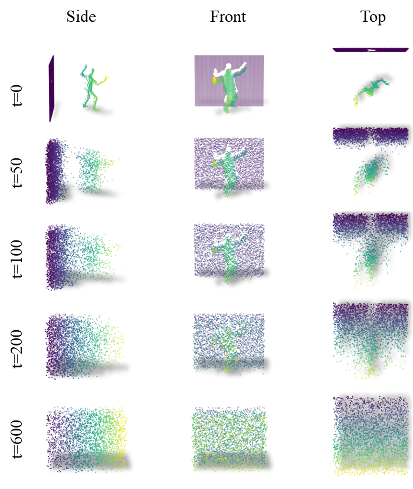
Figure 2: Forward diffusion process of a depth map represented as point cloud $P_{d}$ with a cosine beta schedule and with T=600 diffusion steps. Depth values are scaled to range from -1 to 1, with -1 being the background.

The RGB-D-Fusion framework is depicted in Fig. 3. We input an RGB image of a person with removed background (e.g. captured from a consumer camera device) and output an RGB-D image of that same person, with perspective projection.

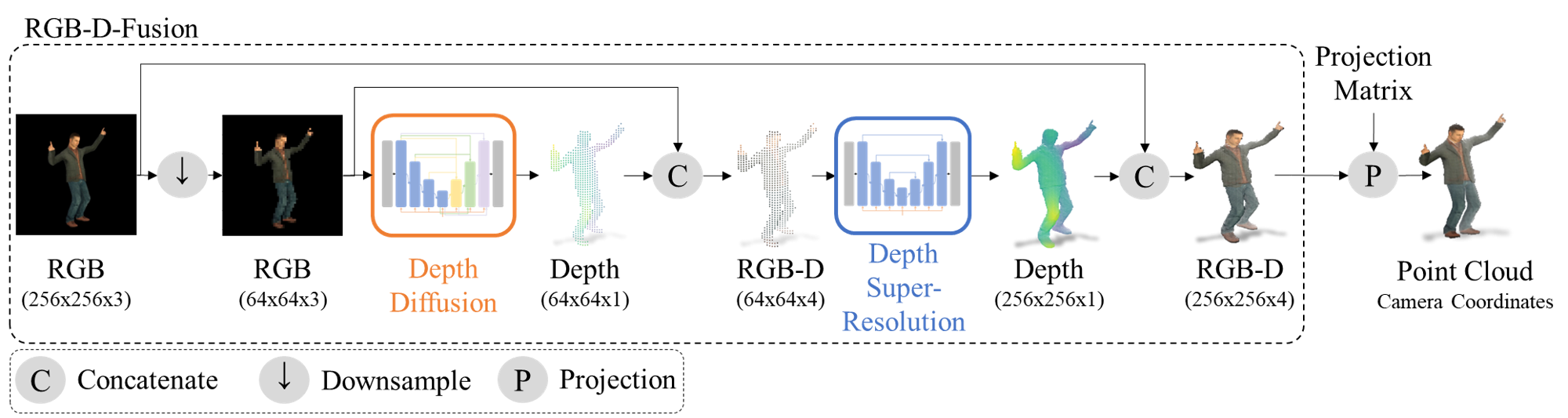
Figure 3: RGB-D-Fusion framework. Our framework takes an RGB image as input and outputs an RGB-D image using perspective projection. We first downsample the input image from 256x256 to 64x64. We then predict the perspective depth map using a conditional denoising diffusion probabilistic model. We then combine the predicted depth map with the input RGB into an RGB-D image of resolution 64x64. We further apply a super-resolution model conditioned on the low-resolution RGB-D to obtain a high-resolution depth map. The predicted high-resolution depth map is combined with the input RGB to construct the final output: a high-resolution RGB-D image. To reconstruct the real depth in camera coordinates, a projection matrix can be applied if available.

Our framework consists of two stages: a depth prediction stage and a depth super-resolution stage. The first stage outputs a low-resolution perspective depth map for a given low-resolution RGB image. The second stage outputs a high-resolution depth map for a given low-resolution RGB-D input.

We first downsample the RGB input to a lower resolution of 64x64 pixels. We resample RGB data using bilinear resampling while for depth maps we apply nearest neighbors resampling to avoid undesired artefacts due to the large gradients introduced of the removed background. We feed the downsampled image into our first stage, a conditional diffusion model (details in section IV-C2) to predict the corresponding depth map. We combine the low-resolution RGB input with the predicted depth map to form an RGB-D image. The low-resolution RGB-D image is fed into our second stage, another conditional diffusion model (details in section IV-C3) to predict a high-resolution depth map. Finally, the predicted depth is combined with the initial RGB input to form the final RGB-D output.

Both our models, the depth diffusion model and the depth super-resolution model, perform the diffusion process on a depth map. The depth diffusion model samples a low-resolution depth map in 64x64 pixels, conditioned on a low-resolution RGB image. Our depth super-resolution model is conditioned on a low-resolution RGB-D image and samples a high-resolution depth map in 256x256 pixels. To obtain the depth in camera coordinates, one must further project the predicted output using a projection matrix if available.

We a apply a cosine beta schedule with $T=600$ for our depth diffusion model and $T=1000$ for our depth super-resolution model. Fig. 2 depicts the forward diffusion of a depth map represented as point cloud for various time steps and viewpoints.

In section V we perform various experiments to ablate and justify our architectural decision now introduced in further detail in section IV-C.

IV-B Dataset

We created a custom dataset by rendering RGB-D images using perspective projection from high-quality 3D models of people (Pagés et al., 2021; Escribano et al., 2022). We randomly varied the camera’s viewpoint, its field of view and its distance to the subject in such a way that the projected person covers 80% of the image’s height. Our dataset contains $\approx$ 25k samples. Each sample contains an RGB image of a person and its corresponding depth map. Both modalities have no background and have a spatial resolution of 256x256. The $\approx$ 25k samples are composed of 358 different subjects. We divide the dataset into a train set with 19,902 samples containing 315 subjects and a test set with 5,302 samples of 43 subjects. For better visualization of the depth maps, we illustrate them as point cloud $P_{d}=\{\left(u_{i},v_{i},z_{i}\right)|i\in N\}$, where $N$ is the number of pixels of the depth map, $u_{i}$ and $v_{i}$ are the pixel coordinates and $d_{i}$ is the depth value. Likewise, an RGB-D image is represented as point cloud $P_{rgbd}=\{\left(u_{i},v_{i},d_{i},r_{i},g_{i},b_{i}\right)|i\in N\}$. In contrast, a colored point cloud in camera coordinates $P_{C}=\{\left(x_{i},y_{i},z_{i},r_{i},g_{i},b_{i}\right)|i\in N\}$ is defined by its 3D coordinates $x_{i}$, $y_{i}$ and $z_{i}$.

IV-C Model Architecture

In this section we provide details on the two models that form our RGB-D-Fusion framework: the RGB conditioned depth diffusion model and the RGB-D conditioned depth super-resolution diffusion model.

IV-C1 Base Model

Before we introduce the individual models we show the base model architecture from which we later derive our depth diffusion model and our depth super-resolution model.

In contrast to previous works (Dhariwal and Nichol, 2021; Nichol and Dhariwal, 2021; Ho et al., 2021) our base model architecture for the depth diffusion model is based on UNet3+ (Huang et al., 2020) and the architecture for our super-resolution model is based on the UNet architecture. A high level comparison is shown in Fig. 4.

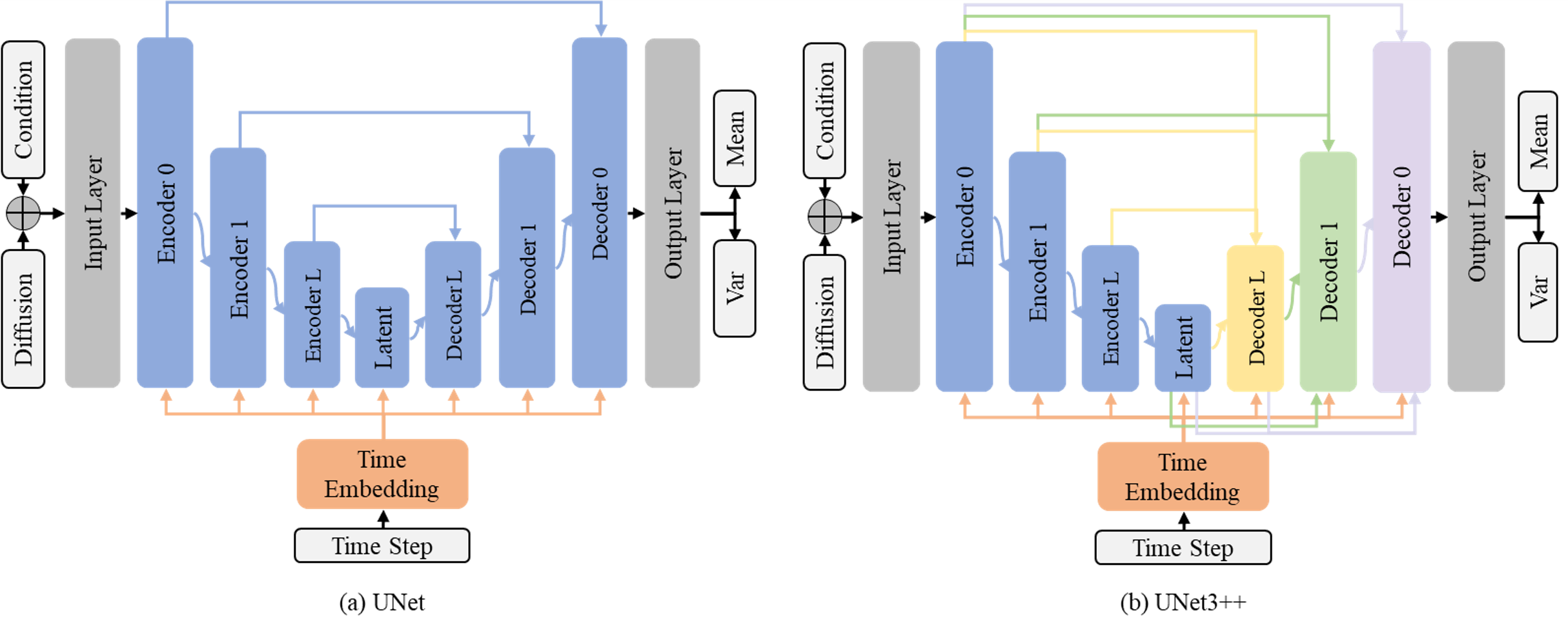
Figure 4: Comparison of our two base architectures. We condition our models on the time step $t$ of the diffusion process and on an additional condition input that is concatenated with the diffusion input. The diffusion input is the noisy sample. During training noise is gradually added to the diffusion input and gradually removed during sampling, while the condition is kept unchanged. Our models predict the mean and the variance of the conditioned diffusion input. The standard UNet architecture depicted in (a) simply connects the encoder and decoder stages with the same spatial resolution, while for the UNet3+ in (b), the decoder is connected to all encoder stages with the same or higher spatial resolution and all decoders with a smaller spatial resolution. Before concatenation, all feature maps are resampled to the same spatial resolution.

Similar to (Dhariwal and Nichol, 2021; Nichol and Dhariwal, 2021) we implement the stages of the model using multiple ResNet blocks followed by an optional multi-head attention block with 8 heads and a hidden dimension of 32 per head. For our latent space stage we implement standard attention by Vaswani et al. (2017) and for stages with higher resolution we implement linear attention as proposed by Wang et al. (2020). We also implement residual up and down-sampling blocks as suggested in BigGAN by Brock et al. (2019). We replace all normalization layers (i.e. batch normalization Ioffe and Szegedy (2015) and instance normalization (Ulyanov et al., 2017)) with group normalization (Wu and He, 2018) with a groupsize of 8 and $\epsilon=1e-05$ and only keep layer normalization (Ba et al., 2016) for all our attention blocks. As suggested by Ioffe and Szegedy (2015), we remove all bias weights from our convolutional layers since the normalization layers introduce a learnable bias. All activations are GeLU (Hendrycks and Gimpel, 2020) except for the softmax activations in the attention blocks. We input the condition via concatenation with the noise input. The time step information is input into each ResNet block (standard as well as in up and down sampling) using adaptive group normalization (AdaGN) (Dhariwal and Nichol, 2021). Following Liu et al. (2022), we increase the number of consecutive ResNet blocks in lower resolution stages and further apply stochastic depth (Huang et al., 2016) during training, to stochastically drop entire ResNet blocks to train an implicit ensemble of models.

IV-C2 RGB Conditioned Depth Diffusion Model

Our depth diffusion model is based on the UNet3+ architecture conditioned on a low-resolution (64x64x3) RGB image and generates a low-resolution depth map (64x64x1) when sampled from. The intention behind this architectural choice is to strengthen the decoder by using inputs from multiple resolutions of the UNet encoder, hence combining local and global features. Corresponding experiments are performed in section V-A.

IV-C3 RGB-D Conditioned Depth Super-Resolution Diffusion Model

Our super-resolution diffusion model is conditioned on a low-resolution (64x64x4) RGB-D image and generates a high-resolution depth map (256x256x1) when sampled from. We use a UNet base architecture as depicted in Fig. 4. The only difference is that before the low-resolution condition is fed into the model, we first upsample to the target resolution to match the resolution of the diffusion input. The RGB-D input is split into RGB and depth map, we then apply bilinear resampling for the RGB image and nearest neighbor resampling for the depth map and finally concatenate to a high-resolution RGB-D image (See Fig. 5). Corresponding experiments are performed in section V-B.

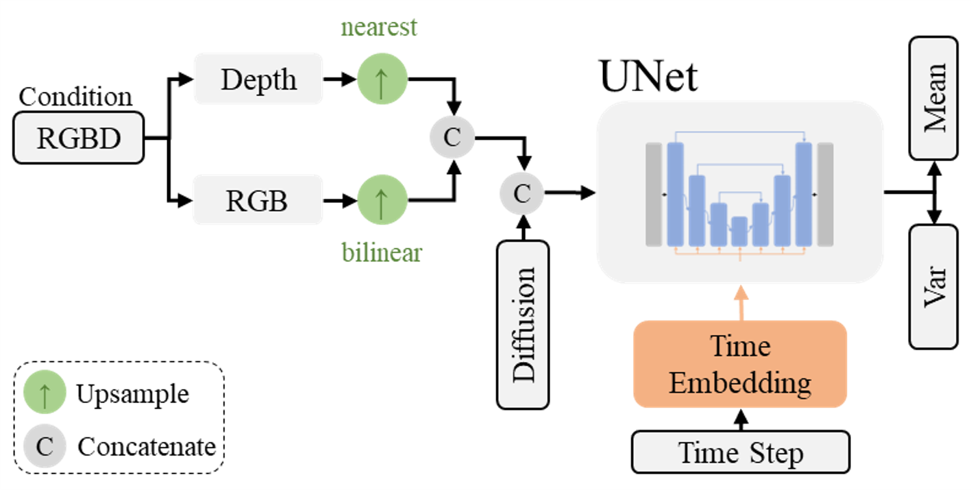
Figure 5: Architecture of our depth super-resolution model. The low-resolution RGB-D image condition is split into its depth and RGB components, upsampled using nearest neighbor and bilinear resampling respectively, and combined again before it is fed into a UNet model.

Compared to our depth diffusion model we make the following two assumptions: first, we assume that super-resolution is an easier task compared to depth estimation conditioned on a different modality, hence less parameters are required to learn this task. Second, high-resolution stages in the UNet architecture are more important than low-resolution stages since it is more important to focus on local features and not to have a global understanding of the image’s content. Based on these assumptions and the fact that higher resolution images require more resources for training, we made the following design changes compared to our depth estimation network: first, we use a the UNet as a base architecture and increase the number of channels in the first stages of the UNet. This gives more importance on high-resolution stages and decreases the importance for low-resolution stages, while at the same time reducing the number of parameters. To extract more features for a given resolution, we increase the number of blocks within each stage. Second, we use the same number of stages in the UNet for our super-resolution from 64 to 128 as for 64 to 256, following the same argumentation of higher importance of high-resolution stages. The reduced number of stages, reduces the number of trainable parameters and computations required for the forward pass and lets us apply a higher batch size, hence speeds up the training and inference time.

IV-D Data Augmentation

During the training of our depth diffusion model we randomly scale and shift the RGB condition input.

For our depth super-resolution model we follow the suggestion of Ho et al. (2021) and augment the RGB condition input with a Gaussian blur by convolving the image with a Gaussian 3x3 kernel with a standard deviation of $\sigma_{rgb}\sim\mathcal{U}_{[0,0.6]}$ with a probability of 0.5 in each epoch:

$$rgb_{aug}=rgb*\epsilon_{rgb}$$ (21)

where $\epsilon_{rgb}\sim\mathcal{N}\left(0,\sigma_{rgb}\right)$, $\epsilon_{rgb}\in\mathbb{R}^{3x3x3}$ and $rgb,rgb_{aug}\in\mathbb{R}^{HxWx3}$

In contrast to Ho et al. (2021), we further provide the depth as a condition input to our super-resolution model. Following the thoughts of Ho et al. (2021) we augment the depth $d$ by adding Gaussian noise with an empirically determined standard deviation of $\sigma_{d}\sim\mathcal{U}_{[0,0.06]}$:

$$d_{aug}=d+\epsilon_{d}$$ (22)

where $\epsilon_{d}\sim\mathcal{N}\left(0,\sigma_{d}\right)$ and $\epsilon_{d},d,d_{aug}\in\mathbb{R}^{HxWx1}$

Fig. 6 shows the comparison of the depth without and with Gaussian additive noise, represented as a point cloud.

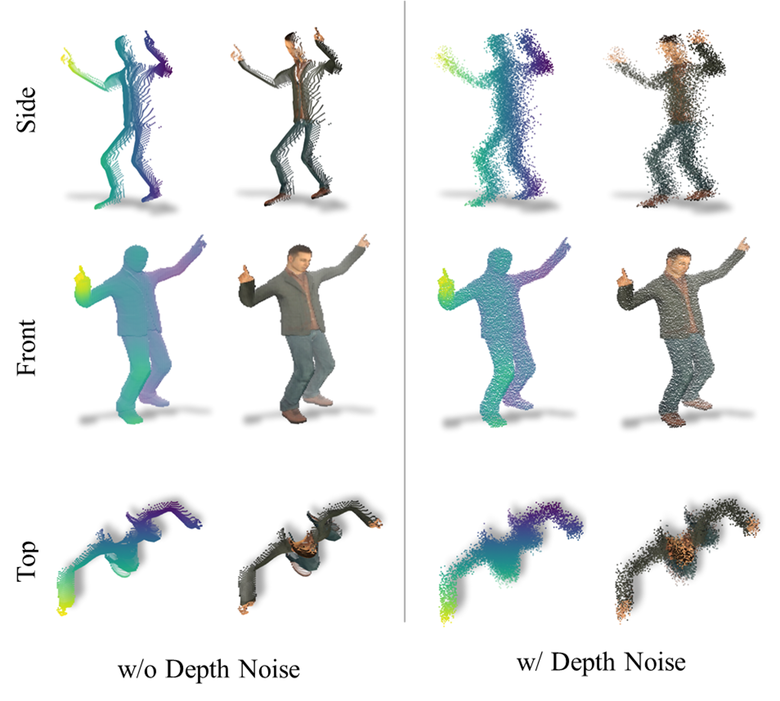
Figure 6: Comparison of a depth sample and an RGB-D sample without depth noise augmentation and with depth noise augmentation represented as point cloud $P_{d}$ and $P_{rgbd}$. We remove the points associated with the background for better representation.

We further apply random scaling and shifting of the RGB-D condition input.

V Experiments

TABLE I: Results of experiments performed with our depth diffusion model. We alter the model architecture, the method to obtain the variance, the loss formulation, the learning rate schedule, the number of residual blocks per stage and the stochastic depth probability. Underlined parameters depict the change compared to the previous run. The detailed architecture of the models can be found in TABLE V in the appendix.

Run	Model	Variance	Loss	$L_{r}$ Schedule	ResBlocks	Stochastic Depth	MAE $\downarrow$	MSE $\downarrow$	IoU $\uparrow$	VLB $\downarrow$
dd1	UNet	fix	simple	x	2/2/2/2	0/0/0/0	8.14	2.57	0.987	10.03
dd2	UNet3+	fix	simple	x	2/2/2/2	0/0/0/0	9.24	2.97	0.988	9.72
dd3	UNet3+	learned	simple	x	2/2/2/2	0/0/0/0	10.83	3.21	0.987	13.00
dd4	UNet3+	learned	P2	x	2/2/2/2	0/0/0/0	8.36	1.75	0.989	14.26
dd5	UNet3+	learned	P2	✓	2/2/2/2	0/0/0/0	7.70	1.58	0.993	12.20
dd6	UNet	learned	P2	✓	2/2/2/2	0/0/0/0	7.45	1.48	0.990	12.39
dd7	UNet	learned	simple	✓	2/2/2/2	0/0/0/0	15.65	8.75	0.946	20.48
dd8	UNet3+	learned	simple	✓	2/2/2/2	0/0/0/0	6.16	1.64	0.993	17.59
dd9	UNet3+	learned	simple	✓	2/2/12/2	0/0/0/0	231.91	251.30	0.539	23.97
dd10	UNet3+	learned	simple	✓	2/2/12/2	0.1/0.1/0.5/0.1	5.79	1.48	0.993	16.95

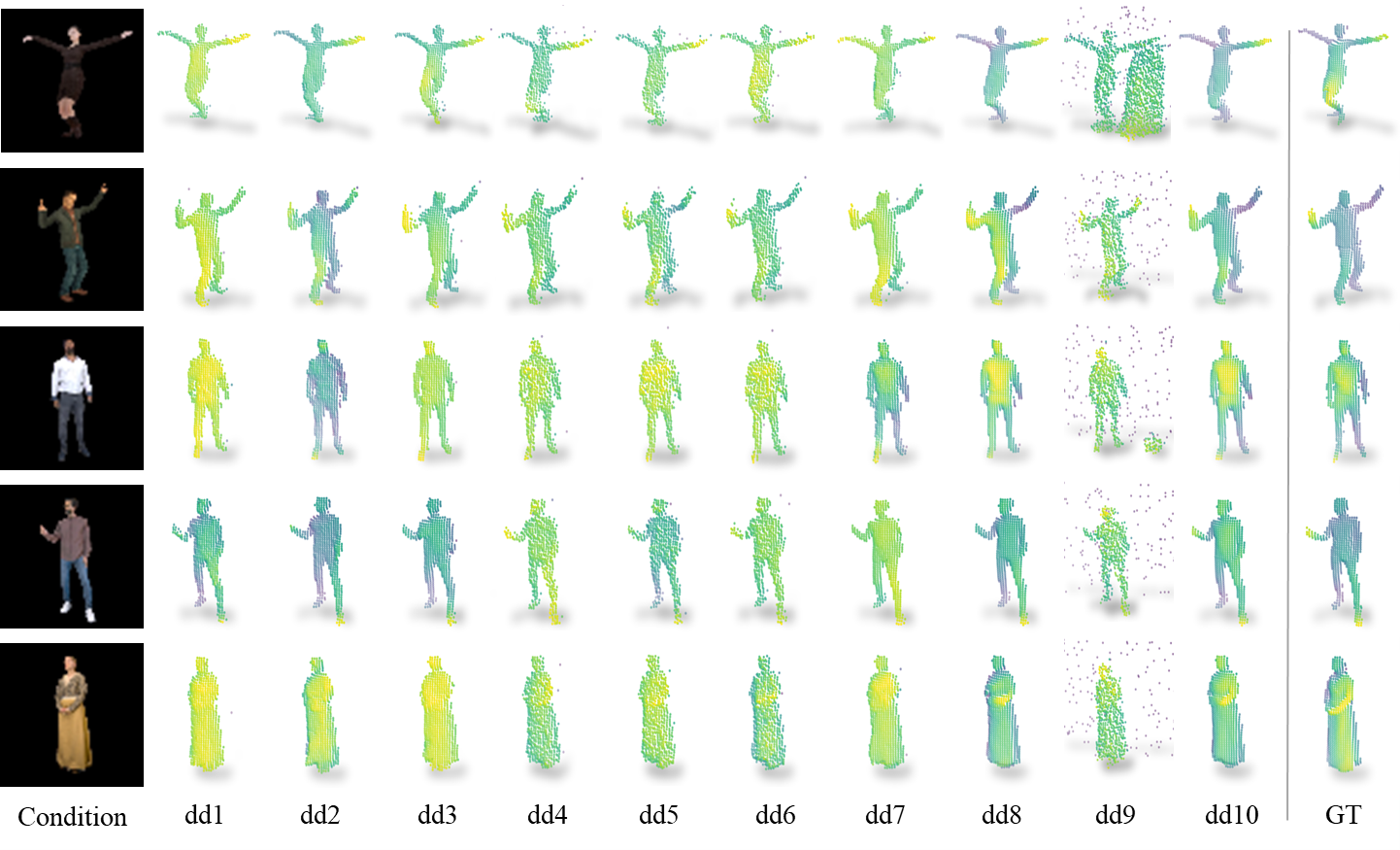
Figure 7: Generated depth maps represented as point clouds $P_{d}$ from our depth diffusion models evaluated in our experiments from TABLE I for each run respectively. To better observe the details, the point clouds’ viewpoint has been rotated 10 degrees in azimuth and 10 degrees in elevation. The color map encodes the depth between the min and max value of the depth of each plot, where darker colors indicate higher depth and brighter colors closer depth.

In this section we perform experiments to validate our design choices. We first run multiple experiments on the conditional depth diffusion network to select various hyperparameters related to model architecture and model training. We incorporate our findings into the conditional depth super-resolution model and find that the best architecture for the depth diffusion is not suitable in terms of resources and performance on the metrics. We hence modify the architecture, investigate on which input modality to condition to and perform an ablation study on the augmentation of the condition input. We evaluate our experiments with the following metrics:

• MAE mean average error distance of the ground truth depth $d_{gt}$ and the predicted depth $d_{pred}$ with $d_{gt},d_{pred}\in\mathbb{R}^{HxWx1}$.

  $$MAE=\frac{1}{n}\sum_{i=1}^{n}\left|d_{gt}-d_{pred}\right|\cdot 10^{3}$$ (23)

  We multiply the result with $10^{3}$. The closer to zero the better.

• MSE mean squared error distance of the ground truth depth $d_{gt}$ and the predicted depth $d_{pred}$.

  $$MSE=\frac{1}{n}\sum_{i=1}^{n}\left(d_{gt}-d_{pred}\right)^{2}\cdot 10^{3}$$ (24)

  We multiply the result with $10^{3}$. The closer to zero the better.

• IoU Intersection over Union calculated over a binary mask $m$ of the ground truth $gt$ and the prediction $p$.

  $$IoU=\frac{m_{gt}\cap m_{p}}{m_{gt}\cup m_{p}},with\;m_{y}=\left\{\begin{array}[]{ll}1,&y>\phi\\ 0,&y\leq\phi\end{array}\right.$$ (25)

  where $\phi$ is the threshold for the binary mask. We set $\phi=-0.95$ since the depth maps range from [-1,1]. The closer to 1 the better.

• VLB of the negative log-likelihood of the test data set (see (9)) reported in bits/dim with base-2 logarithm. The smaller the better.

As highlighted by Theis et al. (2016) the evaluation metrics of generative models are complex and might be misleading especially for high dimensional data like images. High log-likelihood does not imply high sample quality and low log-likelihood does not imply poor samples. Furthermore, an evaluation on samples is claimed to be biased towards overfitting models and favors models of large entropy. We therefore do not rely on a single metric and report the metrics listed above and show samples drawn from the model distribution.

We further want to highlight the weakness of distance metrics like MSE and MAE since the pixel location is of high importance and even a slight shift of a few pixels of two indistinguishable images leads to a high distance metric, as reported by Theis et al. (2016) for a nearest neighbor distance.

All experiments are performed on our test set described in section IV-B which contains $\approx 5300$ data samples.

V-A Depth Diffusion Model

We first investigate the impact of different hyper-parameters on mentioned metrics for our conditional depth diffusion model. Explicitly we perform 10 runs in which we vary the model architecture (UNet vs. UNet3+), the approach for determining the variance (learned range vs. fixed to upper bound $\beta_{t}$), the loss weighting approach (simple vs. P2), a learning rate schedule (no schedule vs. cosine decay with restart and linear warm-up), the number of residual blocks and the usage of stochastic depth augmentation. A detailed summary of the most important hyper parameters for all runs is listed in TABLE V in the appendix.

The results for the conditional depth diffusion models are summarized in TABLE I and outputs of the respective models are depicted in Fig. 7. The underlined parameter highlights the changed configuration compared to the previous run. Best results are printed in bold.

Our baseline (Run 1 in TABLE I) is a UNet model (similar to Dhariwal and Nichol (2021)). The variance is not learned but set to $\beta_{t}$, the upper bound of the reverse diffusion process. We apply the simple loss $L_{simple}$ from equation (14) as our training objective and apply no learning rate schedule.

All runs are trained for 250 epochs using ADAM optimizer with a learning rate $\alpha$ of 4e-5 (exception of Run 5 with $\alpha=6e-5$), $\beta_{1}=0.9$ and $\beta_{2}=0.999$. The forward and the reverse diffusion process is performed with $T=600$ time steps and a cosine noise schedule as in Nichol and Dhariwal (2021). We further apply random scaling and shifting augmentation on the RGB input condition.

Based on the results in TABLE I and the generated images in Fig. 7 we consider run dd10 best.

V-B Depth Super-Resolution Model

We perform various experiments for our super-resolution model. We compare different architectures and ablate the augmentation method. A detailed summary of the most important hyperparameters for all runs is listed in TABLE VI in the appendix.

First, we investigate the impact of the input condition in combination with the model architecture on lower resolution (64 $\rightarrow$ 128) for performance reasons. We condition the model either on a depth map or an RGB-D image. The intuition is that the RGB channels provide further visual glues that are not present in the depth modality and hence improve performance. We further vary number of channels and the diffusion steps $T$. We use two different base architectures; first, we use the UNet3+ from run10 from our depth diffusion experiment (see TABLE I). We refer to this architecture as SR1. We observed slow training performance and low performance on our metrics. Following the intuition that for a super-resolution task the higher levels of the U-Net are more important (where the higher spatial information is present and less semantic information has been extracted), we shift the number of channels from deeper to higher levels and use the U-Net instead of the UNet3+ to remove the connections from various levels. We refer to the adapted architecture as SR2.

TABLE II: Ablation study for our depth super-resolution model where we vary the model base architecture, the input condition format, the base dimension of the model and the number diffusion steps T. Models with T=1000 are trained for 350 epochs, models with T=600 are trained for 250 epochs. All models perform super-resolution from 64x64 to 128x128. The detailed architecture of the models can be found in TABLE VI in the appendix.

Run	Arch.	Cond.	Dim.	T	MAE $\downarrow$	MSE $\downarrow$	IoU $\uparrow$	VLB $\downarrow$
sr1	SR1	RGB-D	96	1000	30.20	29.68	0.815	33.87
sr2	SR1	Depth	64	1000	40.14	39.19	0.789	24.92
sr3	SR1	RGB-D	64	1000	38.70	37.28	0.753	19.48
sr4	SR1	Depth	64	600	30.51	28.39	0.816	20.97
sr5	SR1	RGB-D	64	600	47.32	41.25	0.772	34.93
sr6	SR2	RGB-D	128	1000	3.08	2.66	0.980	10.50
sr7	SR2	Depth	128	1000	5.34	5.07	0.962	10.51
sr8	SR2	RGB-D	128	600	3.26	2.78	0.979	10.34
sr9	SR2	Depth	128	600	5.53	5.20	0.961	10.37
sr10	SR2	RGB-D	192	1000	3.11	2.55	0.981	10.21
sr11	SR2	Depth	192	1000	5.56	5.22	0.961	10.26

In our second experiment we ablate the usage of condition input augmentation, i.e. blurring the RGB using a Gaussian filter (see equation (21)) and applying depth noise (see equation (22)). We report the performance on the metrics in TABLE III. We used the model from run sr6, which is similar to the best run sr10, but requires less compute and hence we can iterate faster. We find that the metrics on our test dataset are slightly worse using any of the augmentations and is worst when applying both. However, we observe that the visual quality of generated samples are better when we input the diffused depth output from our depth diffusion network instead of the GT from the test set. We hypothesize that this might be due to the noisier depth of diffused samples and for those samples, the depth noise augmentation is beneficial.

TABLE III: Ablation study of the augmentation method for our depth super-resolution model. We use model sr6 from TABLE II as our baseline, since it is similar to sr10 but requires less compute, so we can iterate faster. The detailed architecture of the models can be found in TABLE VII in the appendix.

Run	RGB blur	Depth Noise	MAE $\downarrow$	MSE $\downarrow$	IoU $\uparrow$	VLB $\downarrow$
sr6	x	x	3.08	2.66	0.980	10.50
sr61	✓	x	3.91	2.68	0.980	10.47
sr62	x	✓	4.03	2.70	0.980	10.44
sr63	✓	✓	5.60	5.34	0.960	10.49

Finally, we transfer our findings onto training models for higher resolutions, i.e. 64x64 $\rightarrow$ 256x256 and report the performance on the metrics in TABLE IV. We started with run sr12, for which we used the same channel multipliers and number of layers as for sr6. Since attention is a costly operation, we only used it at the same resolutions (i.e. 32x32 and 16x16, because model sr12 does not have 8x8 due to higher input resolution). In run sr121 we added a third level of attention, which kept the VLB roughly equal but improved the IoU, MAE and MSE. With run sr122 we added an extra stage to our U-Net architecture, to verify our hypothesis that lower resolutions do not contribute significantly to the performance of the super-resolution model. The metrics are negligibly better than for sr121 which supports our hypothesis. Based on our results from run sr10, we wanted to test with a base dimensionality of 192 for our higher resolution super-resolution model. We only see minor improvement comparing run sr13 to run sr121. With even worse results for sr131. Since the number of parameters more than doubled from 71M to 161M we think that our dataset is too small and the model overfits on the train set. We consider run sr121 best and select it as final model.

TABLE IV: Ablation study for our depth super-resolution model of the target resolution 64x64 $\rightarrow$ 256x256. We vary the models’ base dimension, the number of stages and its respective base dim multiplier and the respective resolutions where we perform attention. The detailed architecture of the models can be found in TABLE VII in the appendix.

Run	Dim.	Mult.	Att.Res.	MAE $\downarrow$	MSE $\downarrow$	IoU $\uparrow$	VLB $\downarrow$
sr12	128	1/1/2/2/4	16/32	7.73	7.22	0.945	10.34
sr121	128	1/1/2/2/4	16/32/64	4.33	3.02	0.977	10.37
sr122	128	1/1/2/2/4/4	8/16/32	4.30	3.00	0.977	10.37
sr13	192	1/1/2/2/4	16/32	3.54	2.89	0.978	10.06
sr131	192	1/1/2/2/4	16/32/64	17.98	6.04	0.821	9.83

Fig. 8 depicts a visual comparison of our super-resolution model sr121 compared against nearest neighbor upsampling, bilinear upsampling and the ground truth. In Fig. 9 we show the generated outputs at each stage of our RGB-D-Fusion framework.

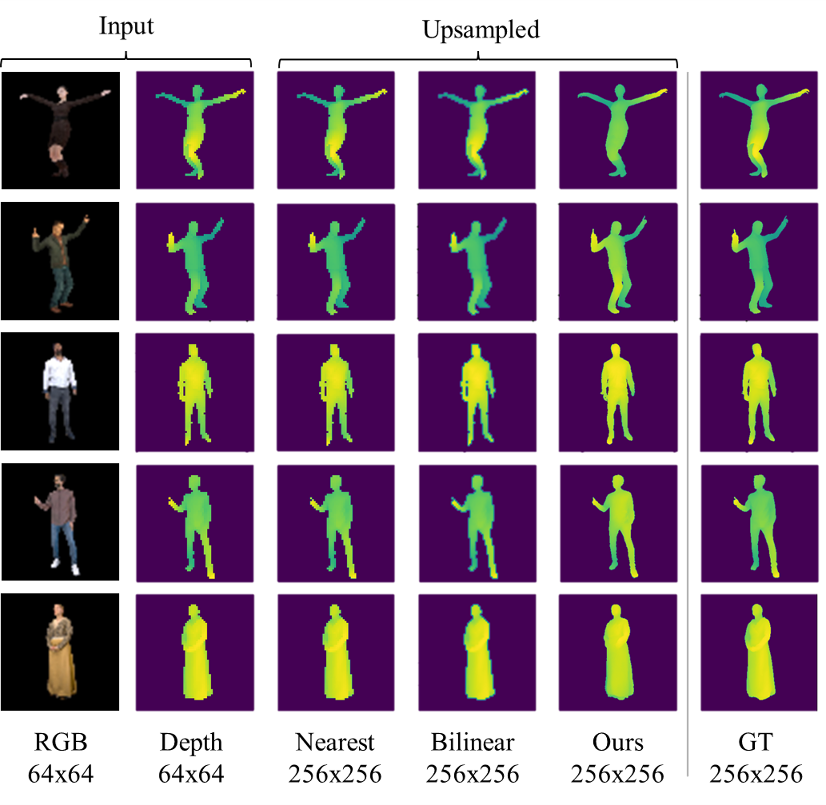
Figure 8: Comparison of our diffusion based depth super-resolution model sr121 against other resampling techniques and the ground truth.

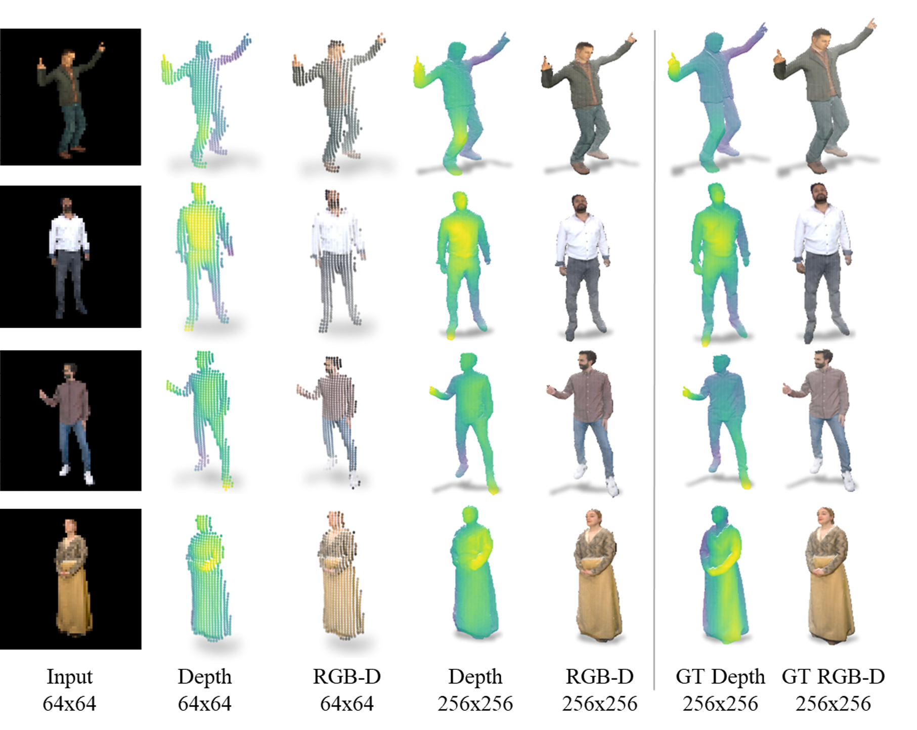
Figure 9: Input and output of our RGB-D-Fusion framework at various stages compared to the ground truth. We use model dd10 for the depth diffusion and sr121 for the depth super-resolution

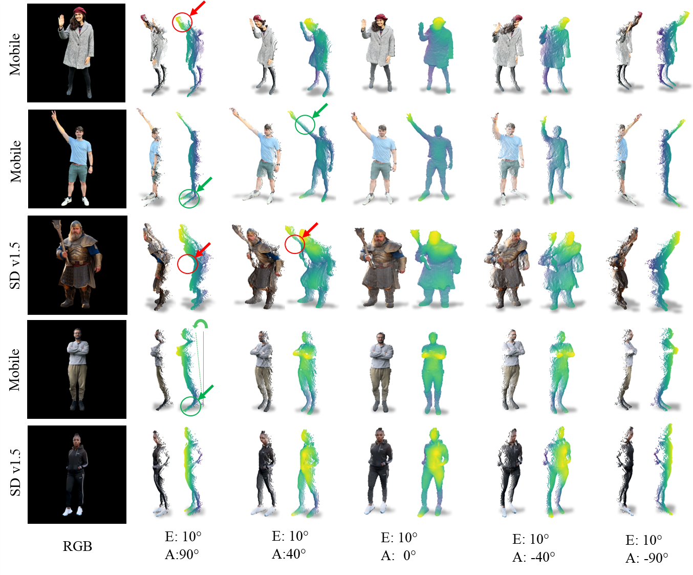
Figure 10: Perspective depth and RGB-D output of our RGB-D-Fusion framework conditioned on RGB images obtained from either mobile cameras or images generated with stable diffusion v1.5. Results are illustrated from different viewpoints, i.e. different elevation angles E and azimuth angles A. Errors and distortions are highlighted in red, while distortions related to perspective projection are highlighted in green.

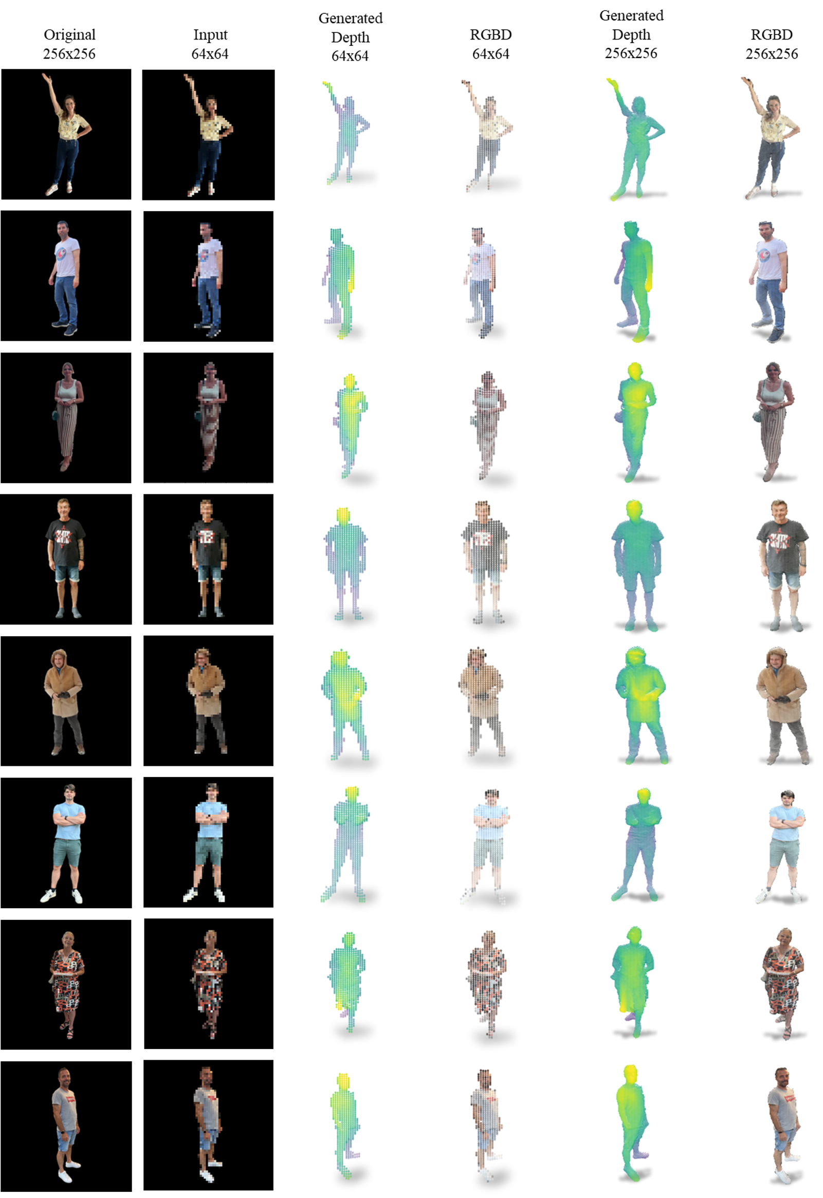
Figure 11: Outputs of the RGB-D-Fusion framework for the given input images. Original images are taken with a variety of single-view mobile cameras.

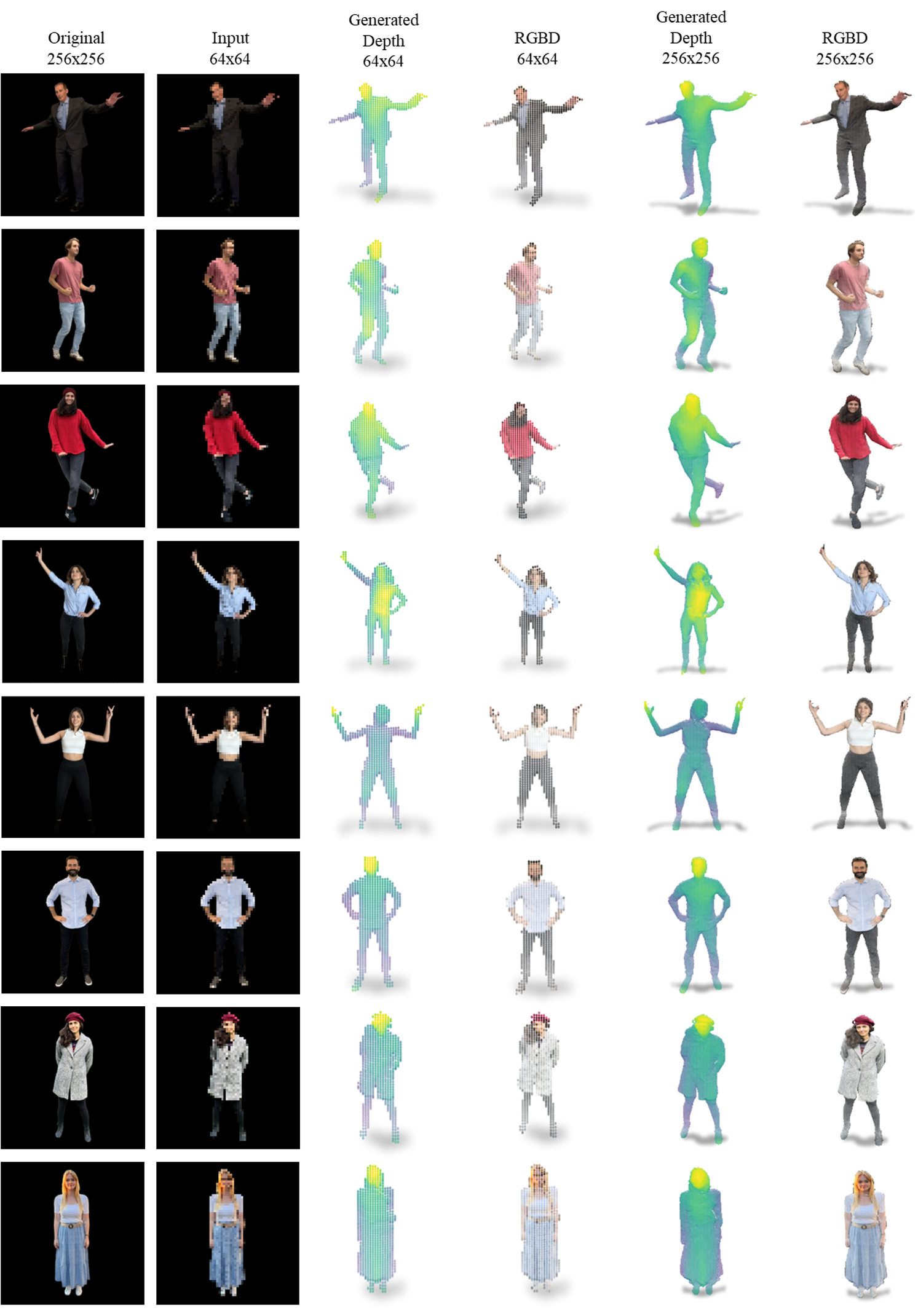
Figure 12: Outputs of the RGB-D-Fusion framework for the given input images. Original images are taken with a variety of single-view mobile cameras.

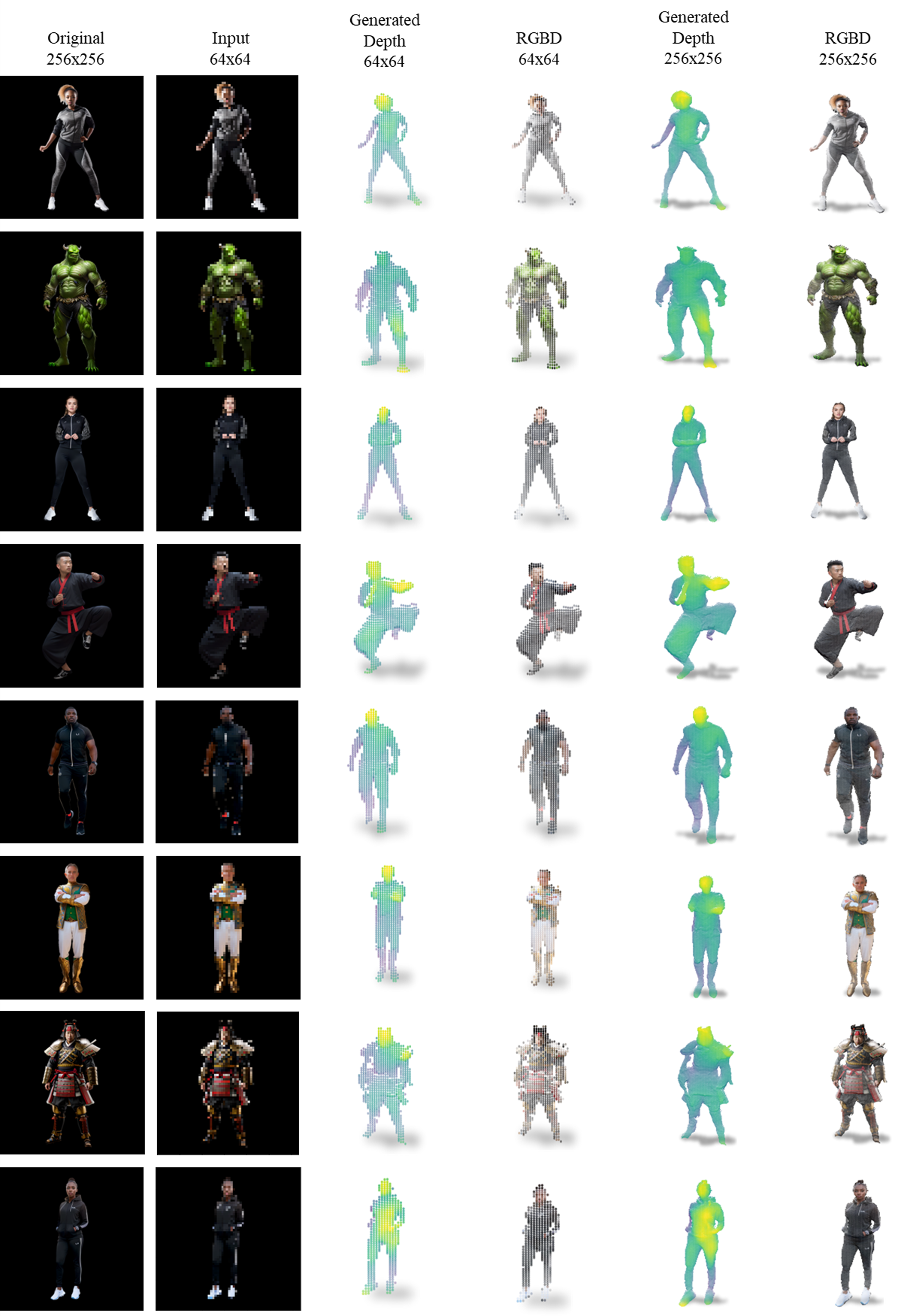
Figure 13: Outputs of the RGB-D-Fusion framework for the given input images. Original images are generated using a stable diffusion model version 1.5 by Rombach et al. (2022).

We further test our RGB-D-Fusion framework on ”in the wild predictions” where we condition the depth diffusion process on RGB images obtained from different mobile cameras and RGB images generated using stable diffusion v1.5 (Rombach et al., 2022). We aim to investigate how well the framework generalizes to RGB images from a different data domain. Some results are shown in Fig. 10 and further results are provided in the appendix in Fig. 11 and Fig. 12 for images obtained from a mobile camera and Fig. 13 for images generated using stable diffusion v1.5.

We observe that for most cases a plausible perspective depth is generated, showing typical distortions such as the subject being tilted towards the camera and lengthen extremities like feet and arms. In some cases the predictions show implausible depths. The super-resolution model on the other hand successfully increases the resolution even of subjects with such implausible depth maps indicating it is robust against domain shifts and solely focusing on increasing the depth maps resolution, which is desirable. We hypothesize that the implausible depth is caused by a large domain gap between the input data and the training data in at least two aspects. First, a domain gap related to the subject’s characteristics like pose, cloths, carried objects as well as lighting and colors in the image. Second, the position and intrinsic parameters of the camera that captured the image are significantly different as those used for rendering our dataset.

VI Conclusion

In this work, we proposed a comprehensive two-staged framework, namely RGB-D-Fusion, to perform monocular depth estimation and depth super-resolution using conditional denoising diffusion probabilistic models. Our depth diffusion model effectively generates depth maps conditioned on low-resolution RGB images in the first stage, while the super-resolution model produces high-resolution depth maps based on a low resolution RGB-D input in the second stage. We introduced a novel depth noise augmentation technique to enhance the robustness of the super-resolution model. Through a series of experiments and ablations we justified design decisions and the effectiveness of our framework and complement those with a variety of generated high resolution RGB-D images.

VI-A Limitations

While our approach generates high-resolution depth maps, the two-stage approach using two consecutive DDPMs leads to a high demand of resources for sampling and training, especially with increasing image resolutions. We observe that for some ”in the wild predictions” the domain gap between input data and training data is to large to generate plausible depth maps indicating a larger dataset might be beneficial. Further, our model outputs a perspective depth which requires a known projection matrix to obtain the depth in any desired coordinate system.

VI-B Future Work

Future research might focus on applying faster sampling algorithms and different model architectures like latent diffusion models which might be promising especially for generating depth maps in higher resolutions. Furthermore, one could extent our approach to directly predict the depth in camera or world coordinates or incorporate camera parameters either into the model architecture or in the pre-processing/augmentation stage of the data pipeline. Further, it would be interesting to investigate different representations for the depth data like point clouds or meshes. Finally, one could also imagine, extending our approach to generate occluded regions of the subject, like it’s back, combining it to a complete 3D model.

Author biographies

Sascha Kirch is a doctoral student at UNED, Spain. His research focuses on self-supervised multi-modal generative deeplearning. He received his M.Sc. degree in Electronic Systems for Communication and Information from UNED, Spain. He received his B.Eng. degree in electrical engineering from the Cooperative State University Baden-Wuerttemberg (DHBW), Germany. Sascha is member of IEEE’s honor society Eta Kappa Nu as part of the chapter Nu Alpha.

Valeria Olyunina is a 3D Computer Vision Engineer at Volograms Ltd. Her work is centered around volumetric reconstruction of people from video, including research into AI-generated shape estimation and other AI applicable to the subject. She received her M.Sc. degree in Computer Science specialising in Augmented Reality from Trinity College Dublin, Ireland. She also has Postgraduate Diploma in Mathematical modelling and Numerical Solutions from University College Cork, Ireland.

Jan Ondřej is Co-Founder and CTO of Volograms, where he has been since 2018. Previously, he was a postdoctoral researcher at Trinity College Dublin and Disney Research Los Angeles. He obtained M.Sc. in Computer Science in 2007 from Czech Technical University in Prague and his Ph.D. in 2011 from INRIA Rennes, in France. Since 2008 he worked as a researcher in several national and European projects related to volumetric video, animation of virtual humans and crowds, and application of VR/AR technologies.

Rafael Pagés is Co-Founder and CEO of Volograms, a startup bringing 3D reconstruction technologies to everyone. He received the Telecommunications Engineering degree (Integrated B.Sc.-M.Sc. accredited by ABET) in 2010, and PhD in Communication Technologies and Systems degree in 2016, both from Technical University of Madrid (UPM), in Spain. Rafael was member of the Image Processing Group at UPM and did his post-doctoral research at Trinity College Dublin. His research interests include 3D reconstruction, volumetric video, and computer vision.

Clara Pérez-Molina received her M.Sc. degree in Physics from the Complutense University in Madrid and her PhD in Industrial Engineering from the Spanish University for Distance Education (UNED). She has worked as researcher in several National and European Projects and has published different technical reports and research articles for International Journals and Conferences, as well as several teaching books. She is currently an Associate Professor with tenure of the Electrical and Computer Engineering Department at UNED. Her research activities are centered on Educational Competences and Technology Enhanced Learning applied to Higher Education in addition to Renewable Energy Management and Artificial Intelligence techniques. She is senior member of the IEEE.

Sergio Martín is Associate Professor at UNED (National University for Distance Education, Spain). He is PhD by the Electrical and Computer Engineering Department of the Industrial Engineering School of UNED. He is Computer Engineer in Distributed Applications and Systems by the Carlos III University of Madrid. He teaches subjects related to microelectronics and digital electronics since 2007 in the Industrial Engineering School of UNED. He has participated since 2002 in national and international research projects related to mobile devices, ambient intelligence, and location-based technologies as well as in projects related to ”e-learning”, virtual and remote labs, and new technologies applied to distance education. He has published more than 200 papers both in international journals and conferences. He is IEEE senior member.

TABLE V: Detailed hyperparameters for depth diffusion models used for experiments in TABLE I

Run	dd1	dd2	dd3	dd4	dd5	dd6	dd7	dd8	dd9	dd10
Model	UNet	UNet3+	UNet3+	UNet3+	UNet3+	UNet	UNet	UNet3+	UNet3+	UNet3+
Diffusion Steps	600	600	600	600	600	600	600	600	600	600
Condition Input	RGB	RGB	RGB	RGB	RGB	RGB	RGB	RGB	RGB	RGB
Noise Schedule	cosine	cosine	cosine	cosine	cosine	cosine	cosine	cosine	cosine	cosine
Model Size	41M	42M	42M	42M	42M	41M	41M	42M	55M	55M
Base Dim	64	64	64	64	64	64	64	64	64	64
Base Dim Mult.	1/2/4/8	1/2/4/8	1/2/4/8	1/2/4/8	1/2/4/8	1/2/4/8	1/2/4/8	1/2/4/8	1/2/4/8	1/2/4/8
# Blocks	1/1/1/1	1/1/1/1	1/1/1/1	1/1/1/1	1/1/1/1	1/1/1/1	1/1/1/1	1/1/1/1	1/1/1/1	1/1/1/1
# ResNet Blocks	2/2/2/2	2/2/2/2	2/2/2/2	2/2/2/2	2/2/2/2	2/2/2/2	2/2/2/2	2/2/2/2	2/2/12/2	2/2/12/2
Stoch. Depth	0/0/0/0	0/0/0/0	0/0/0/0	0/0/0/0	0/0/0/0	0/0/0/0	0/0/0/0	0/0/0/0	0/0/0/0	0.1/0.1/0.5/0.1
Input Resolution	64x64	64x64	64x64	64x64	64x64	64x64	64x64	64x64	64x64	64x64
Output Resolution	64x64	64x64	128x128	64x64	64x64	64x64	64x64	64x64	64x64	64x64
Batch size	128	128	128	128	64	24	24	12	12	12
Variance	fix	fix	learned	learned	learned	learned	learned	learned	learned	learned
Loss Weighting	simple	simple	simple	P2	P2	P2	simple	simple	simple	simple
$L_{r}$	4e-5	4e-5	4e-5	4e-5	6e-5	4e-5	4e-5	4e-5	4e-5	4e-5
$L_{r}$ Schedule	x	x	x	x	✓	✓	✓	✓	✓	✓
Att. Resolution	64/32/16/8	64/32/16/8	64/32/16/8	64/32/16/8	64/32/16/8	64/32/16/8	64/32/16/8	64/32/16/8	64/32/16/8	64/32/16/8
Att. Heads	8	8	8	8	8	8	8	8	8	8
Att. Heads channels	32	32	32	32	32	32	32	32	32	32
GN Group Size	8	8	8	8	8	8	8	8	8	8
Dropout	0.1	0.1	0.1	0.1	0.1	0.1	0.1	0.1	0.1	0.1

TABLE VI: Super-resolution models used for experiments in TABLE II

Run	sr1	sr2	sr3	sr4	sr5	sr6	sr7	sr8	sr9	sr10	sr11
Model	UNet3+	UNet3+	UNet3+	UNet3+	UNet3+	UNet	UNet	UNet	UNet	UNet	UNet
Architecture	SR1	SR1	SR1	SR1	SR1	SR2	SR2	SR2	SR2	SR2	SR2
Diffusion Steps	1000	1000	1000	600	600	1000	1000	600	600	1000	1000
Condition Input	RGB-D	Depth	RGB-D	Depth	RGB-D	RGB-D	Depth	RGB-D	Depth	RGB-D	Depth
Noise Schedule	cosine	cosine	cosine	cosine	cosine	cosine	cosine	cosine	cosine	cosine	cosine
Model Size	153M	69M	69M	69M	69M	72M	72M	72M	72M	161M	161M
Base Dim	96	64	64	64	64	128	128	128	128	192	192
Base Dim Mult.	1/2/4/4/8	1/2/4/4/8	1/2/4/4/8	1/2/4/4/8	1/2/4/4/8	1/1/2/2/4	1/1/2/2/4	1/1/2/2/4	1/1/2/2/4	1/1/2/2/4	1/1/2/2/4
# Blocks	1/1/1/1/1	1/1/1/1/1	1/1/1/1/1	1/1/1/1/1	1/1/1/1/1	1/1/1/1/1	1/1/1/1/1	1/1/1/1/1	1/1/1/1/1	1/1/1/1/1	1/1/1/1/1
# ResNet Blocks	2/2/2/12/2	2/2/2/12/2	2/2/2/12/2	2/2/2/12/2	2/2/2/12/2	3/3/3/3/3	3/3/3/3/3	3/3/3/3/3	3/3/3/3/3	3/3/3/3/3	3/3/3/3/3
Stoch. Depth	0.1/0.1/0.1/0.5/0.1	0.1/0.1/0.1/0.5/0.1	0.1/0.1/0.1/0.5/0.1	0.1/0.1/0.1/0.5/0.1	0.1/0.1/0.1/0.5/0.1	0/0/0/0/0	0/0/0/0/0	0/0/0/0/0	0/0/0/0/0	0/0/0/0/0	0/0/0/0/0
Input Resolution	64x64	64x64	64x64	64x64	64x64	64x64	64x64	64x64	64x64	64x64	64x64
Output Resolution	128x128	128x128	128x128	128x128	128x128	128x128	128x128	128x128	128x128	128x128	128x128
Batch size	8	16	16	16	16	16	16	16	16	8	8
Variance	learned	learned	learned	learned	learned	fix	fix	fix	fix	fix	fix
Loss Weighting	P2	P2	P2	P2	P2	simple	simple	simple	simple	simple	simple
$L_{r}$	1.5e-5	1e-5	1e-5	1e-5	1e-5	5e-5	5e-5	5e-5	5e-5	1e-4	1e-4
$L_{r}$ Schedule	✓	✓	✓	✓	✓	✓	✓	✓	✓	✓	✓
Att. Resolution	32/16/8	32/16/8	32/16/8	32/16/8	32/16/8	32/16/8	32/16/8	32/16/8	32/16/8	32/16/8	32/16/8
Att. Heads	8	8	8	8	8	8	8	8	8	8	8
Att. Heads channels	32	32	32	32	32	32	32	32	32	32	32
GN Group Size	8	8	8	8	8	8	8	8	8	8	8
Dropout	0.1	0.1	0.1	0.1	0.1	0.1	0.1	0.1	0.1	0.1	0.1

TABLE VII: Super-resolution models used for experiments in TABLE III and IV

Run	sr61	sr62	sr63	sr12	sr121	sr122	sr13	sr131
Model	UNet	UNet	UNet	UNet	UNet	UNet	UNet	UNet
Architecture	SR2	SR2	SR2	SR2	SR2	SR2	SR2	SR2
Diffusion Steps	1000	1000	1000	1000	1000	1000	1000	1000
Condition Input	RGB-D	RGB-D	RGB-D	RGB-D	RGB-D	RGB-D	RGB-D	RGB-D
Noise Schedule	cosine	cosine	cosine	cosine	cosine	cosine	cosine	cosine
Model Size	72M	72M	72M	72M	72M	131M	161M	161M
Base Dim	128	128	128	128	128	128	192	192
Base Dim Mult.	1/1/2/2/4	1/1/2/2/4	1/1/2/2/4	1/1/2/2/4	1/1/2/2/4	1/1/2/2/4/4	1/1/2/2/4	1/1/2/2/4
# Blocks	1/1/1/1/1	1/1/1/1/1	1/1/1/1/1/1	1/1/1/1/1	1/1/1/1/1	1/1/1/1/1/1	1/1/1/1/1	1/1/1/1/1
# ResNet Blocks	3/3/3/3/3	3/3/3/3/3	3/3/3/3/3	3/3/3/3/3	3/3/3/3/3	3/3/3/3/3/3	3/3/3/3/3	3/3/3/3/3
Stoch. Depth	0/0/0/0/0	0/0/0/0/0	0/0/0/0/0	0/0/0/0/0	0/0/0/0/0	0/0/0/0/0/0	0/0/0/0/0	0/0/0/0/0
Input Resolution	64x64	64x64	64x64	64x64	64x64	64x64	64x64	64x64
Output Resolution	128x128	128x128	128x128	256x256	256x256	256x256	256x256	256x256
Batch size	16	16	16	4	4	4	2	2
Variance	fix	fix	fix	fix	fix	fix	fix	fix
Loss Weighting	simple	simple	simple	simple	simple	simple	simple	simple
$L_{r}$	5e-5	5e-5	5e-5	3e-5	3e-5	3e-5	5e-5	5e-5
$L_{r}$ Schedule	✓	✓	✓	✓	✓	✓	✓	✓
Att. Resolution	32/16/8	32/16/8	32/16/8	32/16	64/32/16	32/16/8	32/16	64/32/16
Att. Heads	8	8	8	8	8	8	8	8
Att. Heads channels	32	32	32	32	32	32	32	32
GN Group Size	8	8	8	8	8	8	8	8
Dropout	0.1	0.1	0.1	0.1	0.1	0.1	0.1	0.1
Aug. Depth Noise	x	✓	✓	✓	✓	✓	✓	✓
Aug. RGB Blur	✓	x	✓	x	x	x	x	x

References

- Ba et al. (2016) Jimmy Lei Ba, Jamie Ryan Kiros, and Geoffrey E. Hinton. Layer Normalization, July 2016. URL http://arxiv.org/abs/1607.06450. arXiv:1607.06450 [cs, stat].
- Baranchuk et al. (2022) Dmitry Baranchuk, Ivan Rubachev, Andrey Voynov, Valentin Khrulkov, and Artem Babenko. Label-Efficient Semantic Segmentation with Diffusion Models, March 2022. URL http://arxiv.org/abs/2112.03126. arXiv:2112.03126 [cs].
- Batzolis et al. (2021) Georgios Batzolis, Jan Stanczuk, Carola-Bibiane Schönlieb, and Christian Etmann. Conditional Image Generation with Score-Based Diffusion Models, November 2021. URL http://arxiv.org/abs/2111.13606. arXiv:2111.13606 [cs, stat].
- Bhat et al. (2023) Shariq Farooq Bhat, Reiner Birkl, Diana Wofk, Peter Wonka, and Matthias Müller. ZoeDepth: Zero-shot Transfer by Combining Relative and Metric Depth, February 2023. URL http://arxiv.org/abs/2302.12288. arXiv:2302.12288 [cs].
- Bhoi (2019) Amlaan Bhoi. Monocular Depth Estimation: A Survey, January 2019. URL http://arxiv.org/abs/1901.09402. arXiv:1901.09402 [cs].
- Bian et al. (2021) Jia-Wang Bian, Huangying Zhan, Naiyan Wang, Zhichao Li, Le Zhang, Chunhua Shen, Ming-Ming Cheng, and Ian Reid. Unsupervised Scale-consistent Depth Learning from Video. International Journal of Computer Vision, 129(9):2548–2564, September 2021. ISSN 0920-5691, 1573-1405. doi: 10.1007/s11263-021-01484-6. URL http://arxiv.org/abs/2105.11610. arXiv:2105.11610 [cs].
- Brock et al. (2019) Andrew Brock, Jeff Donahue, and Karen Simonyan. Large Scale GAN Training for High Fidelity Natural Image Synthesis, February 2019. URL http://arxiv.org/abs/1809.11096. arXiv:1809.11096 [cs, stat].
- Chen et al. (2018) Long Chen, Wen Tang, and Nigel John. Self-Supervised Monocular Image Depth Learning and Confidence Estimation, March 2018. URL http://arxiv.org/abs/1803.05530. arXiv:1803.05530 [cs].
- Choi et al. (2021) Jooyoung Choi, Sungwon Kim, Yonghyun Jeong, Youngjune Gwon, and Sungroh Yoon. ILVR: Conditioning Method for Denoising Diffusion Probabilistic Models. In 2021 IEEE/CVF International Conference on Computer Vision (ICCV), pages 14347–14356, Montreal, QC, Canada, October 2021. IEEE. ISBN 978-1-66542-812-5. doi: 10.1109/ICCV48922.2021.01410. URL https://ieeexplore.ieee.org/document/9711284/.
- Choi et al. (2022) Jooyoung Choi, Jungbeom Lee, Chaehun Shin, Sungwon Kim, Hyunwoo Kim, and Sungroh Yoon. Perception Prioritized Training of Diffusion Models. In 2022 IEEE/CVF Conference on Computer Vision and Pattern Recognition (CVPR), pages 11462–11471, New Orleans, LA, USA, June 2022. IEEE. ISBN 978-1-66546-946-3. doi: 10.1109/CVPR52688.2022.01118. URL https://ieeexplore.ieee.org/document/9879163/.
- Chung et al. (2022) Hyungjin Chung, Byeongsu Sim, and Jong Chul Ye. Come-Closer-Diffuse-Faster: Accelerating Conditional Diffusion Models for Inverse Problems through Stochastic Contraction. In 2022 IEEE/CVF Conference on Computer Vision and Pattern Recognition (CVPR), pages 12403–12412, New Orleans, LA, USA, June 2022. IEEE. ISBN 978-1-66546-946-3. doi: 10.1109/CVPR52688.2022.01209. URL https://ieeexplore.ieee.org/document/9879691/.
- Collet et al. (2015) Alvaro Collet, Ming Chuang, Pat Sweeney, Don Gillett, Dennis Evseev, David Calabrese, Hugues Hoppe, Adam Kirk, and Steve Sullivan. High-quality streamable free-viewpoint video. ACM Transactions on Graphics (ToG), 34(4):1–13, 2015.
- Dhariwal and Nichol (2021) Prafulla Dhariwal and Alex Nichol. Diffusion Models Beat GANs on Image Synthesis, June 2021. URL http://arxiv.org/abs/2105.05233. arXiv:2105.05233 [cs, stat].
- Dinh et al. (2017) Laurent Dinh, Jascha Sohl-Dickstein, and Samy Bengio. Density estimation using Real NVP, February 2017. URL http://arxiv.org/abs/1605.08803. arXiv:1605.08803 [cs, stat].
- Duan et al. (2023) Yiqun Duan, Zheng Zhu, and Xianda Guo. DiffusionDepth: Diffusion Denoising Approach for Monocular Depth Estimation, March 2023. URL http://arxiv.org/abs/2303.05021. arXiv:2303.05021 [cs].
- Durkan et al. (2019) Conor Durkan, Artur Bekasov, Iain Murray, and George Papamakarios. Neural Spline Flows, December 2019. URL http://arxiv.org/abs/1906.04032. arXiv:1906.04032 [cs, stat].
- Eldesokey et al. (2020) Abdelrahman Eldesokey, Michael Felsberg, and Fahad Shahbaz Khan. Confidence Propagation through CNNs for Guided Sparse Depth Regression. IEEE Transactions on Pattern Analysis and Machine Intelligence, 42(10):2423–2436, October 2020. ISSN 0162-8828, 2160-9292, 1939-3539. doi: 10.1109/TPAMI.2019.2929170. URL http://arxiv.org/abs/1811.01791. arXiv:1811.01791 [cs].
- Escribano et al. (2022) Jorge González Escribano, Susana Ruano, Archana Swaminathan, David Smyth, and Aljosa Smolic. Texture improvement for human shape estimation from a single image. In 24th Irish Machine Vision and Image Processing Conference, 2022.
- Goodfellow et al. (2014) Ian J. Goodfellow, Jean Pouget-Abadie, Mehdi Mirza, Bing Xu, David Warde-Farley, Sherjil Ozair, Aaron Courville, and Yoshua Bengio. Generative Adversarial Networks, June 2014. URL http://arxiv.org/abs/1406.2661. arXiv:1406.2661 [cs, stat].
- Gu et al. (2022) Shuyang Gu, Dong Chen, Jianmin Bao, Fang Wen, Bo Zhang, Dongdong Chen, Lu Yuan, and Baining Guo. Vector Quantized Diffusion Model for Text-to-Image Synthesis, March 2022. URL http://arxiv.org/abs/2111.14822. arXiv:2111.14822 [cs].
- Guo et al. (2019) Kaiwen Guo, Peter Lincoln, Philip Davidson, Jay Busch, Xueming Yu, Matt Whalen, Geoff Harvey, Sergio Orts-Escolano, Rohit Pandey, Jason Dourgarian, et al. The relightables: Volumetric performance capture of humans with realistic relighting. ACM Transactions on Graphics (ToG), 38(6):1–19, 2019.
- Harvey et al. (2022) William Harvey, Saeid Naderiparizi, Vaden Masrani, Christian Weilbach, and Frank Wood. Flexible Diffusion Modeling of Long Videos, December 2022. URL http://arxiv.org/abs/2205.11495. arXiv:2205.11495 [cs].
- Hendrycks and Gimpel (2020) Dan Hendrycks and Kevin Gimpel. Gaussian Error Linear Units (GELUs), July 2020. URL http://arxiv.org/abs/1606.08415. arXiv:1606.08415.
- Ho and Salimans (2022) Jonathan Ho and Tim Salimans. Classifier-Free Diffusion Guidance, July 2022. URL http://arxiv.org/abs/2207.12598. arXiv:2207.12598 [cs].
- Ho et al. (2020) Jonathan Ho, Ajay Jain, and Pieter Abbeel. Denoising Diffusion Probabilistic Models, 2020. URL http://arxiv.org/abs/2006.11239. arXiv:2006.11239 [cs, stat].
- Ho et al. (2021) Jonathan Ho, Chitwan Saharia, William Chan, David J. Fleet, Mohammad Norouzi, and Tim Salimans. Cascaded Diffusion Models for High Fidelity Image Generation, December 2021. URL http://arxiv.org/abs/2106.15282. arXiv:2106.15282 [cs].
- Ho et al. (2022) Jonathan Ho, Tim Salimans, Alexey Gritsenko, William Chan, Mohammad Norouzi, and David J. Fleet. Video Diffusion Models, June 2022. URL http://arxiv.org/abs/2204.03458. arXiv:2204.03458 [cs].
- Huang et al. (2016) Gao Huang, Yu Sun, Zhuang Liu, Daniel Sedra, and Kilian Weinberger. Deep Networks with Stochastic Depth, July 2016. URL http://arxiv.org/abs/1603.09382. arXiv:1603.09382 [cs].
- Huang et al. (2020) Huimin Huang, Lanfen Lin, Ruofeng Tong, Hongjie Hu, Qiaowei Zhang, Yutaro Iwamoto, Xianhua Han, Yen-Wei Chen, and Jian Wu. UNet 3+: A Full-Scale Connected UNet for Medical Image Segmentation, April 2020. URL http://arxiv.org/abs/2004.08790. arXiv:2004.08790.
- Ioffe and Szegedy (2015) Sergey Ioffe and Christian Szegedy. Batch Normalization: Accelerating Deep Network Training by Reducing Internal Covariate Shift, March 2015. URL http://arxiv.org/abs/1502.03167. arXiv:1502.03167 [cs].
- Karras et al. (2019) Tero Karras, Samuli Laine, and Timo Aila. A Style-Based Generator Architecture for Generative Adversarial Networks, March 2019. URL http://arxiv.org/abs/1812.04948. arXiv:1812.04948 [cs, stat].
- Karras et al. (2022) Tero Karras, Miika Aittala, Timo Aila, and Samuli Laine. Elucidating the Design Space of Diffusion-Based Generative Models, October 2022. URL http://arxiv.org/abs/2206.00364. arXiv:2206.00364 [cs, stat].
- Khan et al. (2021) Numair Khan, Min H. Kim, and James Tompkin. Differentiable Diffusion for Dense Depth Estimation from Multi-view Images. In 2021 IEEE/CVF Conference on Computer Vision and Pattern Recognition (CVPR), pages 8908–8917, Nashville, TN, USA, June 2021. IEEE. ISBN 978-1-66544-509-2. doi: 10.1109/CVPR46437.2021.00880. URL https://ieeexplore.ieee.org/document/9577844/.
- Kim et al. (2023) Gyeongnyeon Kim, Wooseok Jang, Gyuseong Lee, Susung Hong, Junyoung Seo, and Seungryong Kim. DAG: Depth-Aware Guidance with Denoising Diffusion Probabilistic Models, January 2023. URL http://arxiv.org/abs/2212.08861. arXiv:2212.08861 [cs].
- Kingma and Welling (2022) Diederik P. Kingma and Max Welling. Auto-Encoding Variational Bayes, December 2022. URL http://arxiv.org/abs/1312.6114. arXiv:1312.6114 [cs, stat].
- Kingma et al. (2022) Diederik P. Kingma, Tim Salimans, Ben Poole, and Jonathan Ho. Variational Diffusion Models, December 2022. URL http://arxiv.org/abs/2107.00630. arXiv:2107.00630 [cs, stat].
- Kirch et al. (2022) Sascha Kirch, Rafael Pagés, Sergio Arnaldo, and Sergio Martín. VoloGAN: Adversarial Domain Adaptation for Synthetic Depth Data, July 2022. URL http://arxiv.org/abs/2207.09204. arXiv:2207.09204 [cs, eess].
- Kong et al. (2021) Zhifeng Kong, Wei Ping, Jiaji Huang, Kexin Zhao, and Bryan Catanzaro. DiffWave: A Versatile Diffusion Model for Audio Synthesis, March 2021. URL http://arxiv.org/abs/2009.09761. arXiv:2009.09761 [cs, eess, stat].
- Lee et al. (2022) Sang-gil Lee, Heeseung Kim, Chaehun Shin, Xu Tan, Chang Liu, Qi Meng, Tao Qin, Wei Chen, Sungroh Yoon, and Tie-Yan Liu. PriorGrad: Improving Conditional Denoising Diffusion Models with Data-Dependent Adaptive Prior, February 2022. URL http://arxiv.org/abs/2106.06406. arXiv:2106.06406 [cs, eess, stat].
- Liu et al. (2021a) Andrew Liu, Richard Tucker, Varun Jampani, Ameesh Makadia, Noah Snavely, and Angjoo Kanazawa. Infinite Nature: Perpetual View Generation of Natural Scenes from a Single Image, November 2021a. URL http://arxiv.org/abs/2012.09855. arXiv:2012.09855 [cs].
- Liu et al. (2020) Haojie Liu, Kang Liao, Chunyu Lin, Yao Zhao, and Yulan Guo. Pseudo-LiDAR Point Cloud Interpolation Based on 3D Motion Representation and Spatial Supervision, June 2020. URL http://arxiv.org/abs/2006.11481. arXiv:2006.11481 [cs].
- Liu et al. (2021b) Ze Liu, Yutong Lin, Yue Cao, Han Hu, Yixuan Wei, Zheng Zhang, Stephen Lin, and Baining Guo. Swin Transformer: Hierarchical Vision Transformer using Shifted Windows, August 2021b. URL http://arxiv.org/abs/2103.14030. arXiv:2103.14030 [cs].
- Liu et al. (2022) Zhuang Liu, Hanzi Mao, Chao-Yuan Wu, Christoph Feichtenhofer, Trevor Darrell, and Saining Xie. A ConvNet for the 2020s, March 2022. URL http://arxiv.org/abs/2201.03545. arXiv:2201.03545 [cs].
- Lu et al. (2022) Keyu Lu, Chengyi Zeng, and Yonghu Zeng. Self-supervised learning of monocular depth using quantized networks. Neurocomputing, 488:634–646, June 2022. ISSN 0925-2312. doi: 10.1016/j.neucom.2021.11.071. URL https://www.sciencedirect.com/science/article/pii/S0925231221017483.
- Luo and Hu (2021) Shitong Luo and Wei Hu. Diffusion Probabilistic Models for 3D Point Cloud Generation, June 2021. URL http://arxiv.org/abs/2103.01458. arXiv:2103.01458 [cs].
- Masoumian et al. (2022) Armin Masoumian, Hatem A. Rashwan, Julián Cristiano, M. Salman Asif, and Domenec Puig. Monocular Depth Estimation Using Deep Learning: A Review. Sensors, 22(14):5353, July 2022. ISSN 1424-8220. doi: 10.3390/s22145353. URL https://www.mdpi.com/1424-8220/22/14/5353.
- Meng et al. (2022) Chenlin Meng, Yutong He, Yang Song, Jiaming Song, Jiajun Wu, Jun-Yan Zhu, and Stefano Ermon. SDEdit: Guided Image Synthesis and Editing with Stochastic Differential Equations, January 2022. URL http://arxiv.org/abs/2108.01073. arXiv:2108.01073 [cs].
- Mildenhall et al. (2021) Ben Mildenhall, Pratul P Srinivasan, Matthew Tancik, Jonathan T Barron, Ravi Ramamoorthi, and Ren Ng. Nerf: Representing scenes as neural radiance fields for view synthesis. Communications of the ACM, 65(1):99–106, 2021.
- Ming et al. (2021) Yue Ming, Xuyang Meng, Chunxiao Fan, and Hui Yu. Deep learning for monocular depth estimation: A review. Neurocomputing, 438:14–33, May 2021. ISSN 0925-2312. doi: 10.1016/j.neucom.2020.12.089. URL https://www.sciencedirect.com/science/article/pii/S0925231220320014.
- Nichol and Dhariwal (2021) Alex Nichol and Prafulla Dhariwal. Improved Denoising Diffusion Probabilistic Models, February 2021. URL http://arxiv.org/abs/2102.09672. arXiv:2102.09672 [cs, stat].
- Nichol et al. (2022a) Alex Nichol, Prafulla Dhariwal, Aditya Ramesh, Pranav Shyam, Pamela Mishkin, Bob McGrew, Ilya Sutskever, and Mark Chen. Towards Photorealistic Image Generation and Editing with Text-Guided Diffusion Models, March 2022a. URL http://arxiv.org/abs/2112.10741. arXiv:2112.10741 [cs].
- Nichol et al. (2022b) Alex Nichol, Heewoo Jun, Prafulla Dhariwal, Pamela Mishkin, and Mark Chen. Point-E: A System for Generating 3D Point Clouds from Complex Prompts, December 2022b. URL http://arxiv.org/abs/2212.08751. arXiv:2212.08751 [cs].
- Pagés et al. (2018) Rafael Pagés, Konstantinos Amplianitis, David Monaghan, Jan Ondřej, and Aljosa Smolić. Affordable content creation for free-viewpoint video and vr/ar applications. Journal of Visual Communication and Image Representation, 53:192–201, 2018.
- Pagés et al. (2021) Rafael Pagés, Emin Zerman, Konstantinos Amplianitis, Jan Ondřej, and Aljosa Smolic. Volograms & V-SENSE Volumetric Video Dataset. ISO/IEC JTC1/SC29/WG07 MPEG2021/m56767, 2021.
- Piao et al. (2021) Yongri Piao, Yukun Zhang, Miao Zhang, and Xinxin Ji. Dynamic Fusion Network For Light Field Depth Estimation, April 2021. URL http://arxiv.org/abs/2104.05969. arXiv:2104.05969 [cs].
- Poole et al. (2022) Ben Poole, Ajay Jain, Jonathan T. Barron, and Ben Mildenhall. DreamFusion: Text-to-3D using 2D Diffusion, September 2022. URL http://arxiv.org/abs/2209.14988. arXiv:2209.14988 [cs, stat].
- Preechakul et al. (2022) Konpat Preechakul, Nattanat Chatthee, Suttisak Wizadwongsa, and Supasorn Suwajanakorn. Diffusion Autoencoders: Toward a Meaningful and Decodable Representation, March 2022. URL http://arxiv.org/abs/2111.15640. arXiv:2111.15640 [cs].
- Ramesh et al. (2022) Aditya Ramesh, Prafulla Dhariwal, Alex Nichol, Casey Chu, and Mark Chen. Hierarchical Text-Conditional Image Generation with CLIP Latents, April 2022. URL http://arxiv.org/abs/2204.06125. arXiv:2204.06125 [cs].
- Rampas et al. (2023) Dominic Rampas, Pablo Pernias, and Marc Aubreville. A Novel Sampling Scheme for Text- and Image-Conditional Image Synthesis in Quantized Latent Spaces, May 2023. URL http://arxiv.org/abs/2211.07292. arXiv:2211.07292 [cs].
- Ranftl et al. (2020) René Ranftl, Katrin Lasinger, David Hafner, Konrad Schindler, and Vladlen Koltun. Towards Robust Monocular Depth Estimation: Mixing Datasets for Zero-shot Cross-dataset Transfer, August 2020. URL http://arxiv.org/abs/1907.01341. arXiv:1907.01341 [cs].
- Razavi et al. (2019) Ali Razavi, Aaron van den Oord, and Oriol Vinyals. Generating Diverse High-Fidelity Images with VQ-VAE-2, June 2019. URL http://arxiv.org/abs/1906.00446. arXiv:1906.00446 [cs, stat].
- Rockwell et al. (2021) Chris Rockwell, David F. Fouhey, and Justin Johnson. PixelSynth: Generating a 3D-Consistent Experience from a Single Image, August 2021. URL http://arxiv.org/abs/2108.05892. arXiv:2108.05892 [cs].
- Rombach et al. (2022) Robin Rombach, Andreas Blattmann, Dominik Lorenz, Patrick Esser, and Björn Ommer. High-Resolution Image Synthesis with Latent Diffusion Models, April 2022. URL http://arxiv.org/abs/2112.10752. arXiv:2112.10752 [cs].
- Ruan et al. (2023) Ludan Ruan, Yiyang Ma, Huan Yang, Huiguo He, Bei Liu, Jianlong Fu, Nicholas Jing Yuan, Qin Jin, and Baining Guo. MM-Diffusion: Learning Multi-Modal Diffusion Models for Joint Audio and Video Generation, March 2023. URL http://arxiv.org/abs/2212.09478. arXiv:2212.09478 [cs].
- Saharia et al. (2021) Chitwan Saharia, Jonathan Ho, William Chan, Tim Salimans, David J. Fleet, and Mohammad Norouzi. Image Super-Resolution via Iterative Refinement, June 2021. URL http://arxiv.org/abs/2104.07636. arXiv:2104.07636 [cs, eess].
- Saharia et al. (2022a) Chitwan Saharia, William Chan, Huiwen Chang, Chris A. Lee, Jonathan Ho, Tim Salimans, David J. Fleet, and Mohammad Norouzi. Palette: Image-to-Image Diffusion Models, May 2022a. URL http://arxiv.org/abs/2111.05826. arXiv:2111.05826 [cs].
- Saharia et al. (2022b) Chitwan Saharia, William Chan, Saurabh Saxena, Lala Li, Jay Whang, Emily Denton, Seyed Kamyar Seyed Ghasemipour, Burcu Karagol Ayan, S. Sara Mahdavi, Rapha Gontijo Lopes, Tim Salimans, Jonathan Ho, David J. Fleet, and Mohammad Norouzi. Photorealistic Text-to-Image Diffusion Models with Deep Language Understanding, May 2022b. URL http://arxiv.org/abs/2205.11487. arXiv:2205.11487 [cs].
- Saito et al. (2019) Shunsuke Saito, Zeng Huang, Ryota Natsume, Shigeo Morishima, Angjoo Kanazawa, and Hao Li. Pifu: Pixel-aligned implicit function for high-resolution clothed human digitization. In Proceedings of the IEEE/CVF international conference on computer vision, pages 2304–2314, 2019.
- Saito et al. (2020) Shunsuke Saito, Tomas Simon, Jason Saragih, and Hanbyul Joo. Pifuhd: Multi-level pixel-aligned implicit function for high-resolution 3d human digitization. In Proceedings of the IEEE/CVF Conference on Computer Vision and Pattern Recognition, pages 84–93, 2020.
- Salimans and Ho (2022) Tim Salimans and Jonathan Ho. Progressive Distillation for Fast Sampling of Diffusion Models, June 2022. URL http://arxiv.org/abs/2202.00512. arXiv:2202.00512 [cs, stat].
- Saxena et al. (2023) Saurabh Saxena, Abhishek Kar, Mohammad Norouzi, and David J. Fleet. Monocular Depth Estimation using Diffusion Models, February 2023. URL http://arxiv.org/abs/2302.14816. arXiv:2302.14816 [cs].
- Sinha et al. (2021) Abhishek Sinha, Jiaming Song, Chenlin Meng, and Stefano Ermon. D2C: Diffusion-Denoising Models for Few-shot Conditional Generation, June 2021. URL http://arxiv.org/abs/2106.06819. arXiv:2106.06819 [cs].
- Sohl-Dickstein et al. (2015) Jascha Sohl-Dickstein, Eric A. Weiss, Niru Maheswaranathan, and Surya Ganguli. Deep Unsupervised Learning using Nonequilibrium Thermodynamics, November 2015. URL http://arxiv.org/abs/1503.03585. arXiv:1503.03585 [cond-mat, q-bio, stat].
- Song et al. (2022) Jiaming Song, Chenlin Meng, and Stefano Ermon. Denoising Diffusion Implicit Models, October 2022. URL http://arxiv.org/abs/2010.02502. arXiv:2010.02502 [cs].
- Song and Ermon (2020) Yang Song and Stefano Ermon. Improved Techniques for Training Score-Based Generative Models, October 2020. URL http://arxiv.org/abs/2006.09011. arXiv:2006.09011 [cs, stat].
- Song et al. (2021a) Yang Song, Conor Durkan, Iain Murray, and Stefano Ermon. Maximum Likelihood Training of Score-Based Diffusion Models, October 2021a. URL http://arxiv.org/abs/2101.09258. arXiv:2101.09258 [cs, stat].
- Song et al. (2021b) Yang Song, Jascha Sohl-Dickstein, Diederik P. Kingma, Abhishek Kumar, Stefano Ermon, and Ben Poole. Score-Based Generative Modeling through Stochastic Differential Equations, February 2021b. URL http://arxiv.org/abs/2011.13456. arXiv:2011.13456 [cs, stat].
- Tang et al. (2023) Zhicong Tang, Shuyang Gu, Jianmin Bao, Dong Chen, and Fang Wen. Improved Vector Quantized Diffusion Models, February 2023. URL http://arxiv.org/abs/2205.16007. arXiv:2205.16007 [cs].
- Theis et al. (2016) Lucas Theis, Aäron van den Oord, and Matthias Bethge. A note on the evaluation of generative models, April 2016. URL http://arxiv.org/abs/1511.01844. arXiv:1511.01844 [cs, stat].
- Ulyanov et al. (2017) Dmitry Ulyanov, Andrea Vedaldi, and Victor Lempitsky. Instance Normalization: The Missing Ingredient for Fast Stylization, November 2017. URL http://arxiv.org/abs/1607.08022. arXiv:1607.08022 [cs].
- Vaswani et al. (2017) Ashish Vaswani, Noam Shazeer, Niki Parmar, Jakob Uszkoreit, Llion Jones, Aidan N. Gomez, Lukasz Kaiser, and Illia Polosukhin. Attention Is All You Need, December 2017. URL http://arxiv.org/abs/1706.03762. arXiv:1706.03762 [cs].
- Wang et al. (2020) Sinong Wang, Belinda Z. Li, Madian Khabsa, Han Fang, and Hao Ma. Linformer: Self-Attention with Linear Complexity, June 2020. URL http://arxiv.org/abs/2006.04768. arXiv:2006.04768 [cs, stat].
- Watson et al. (2022) Daniel Watson, William Chan, Ricardo Martin-Brualla, Jonathan Ho, Andrea Tagliasacchi, and Mohammad Norouzi. Novel View Synthesis with Diffusion Models, October 2022. URL http://arxiv.org/abs/2210.04628. arXiv:2210.04628 [cs].
- Watson et al. (2021) Jamie Watson, Oisin Mac Aodha, Victor Prisacariu, Gabriel Brostow, and Michael Firman. The Temporal Opportunist: Self-Supervised Multi-Frame Monocular Depth, July 2021. URL http://arxiv.org/abs/2104.14540. arXiv:2104.14540 [cs].
- Wu and He (2018) Yuxin Wu and Kaiming He. Group Normalization, June 2018. URL http://arxiv.org/abs/1803.08494. arXiv:1803.08494.
- Xiao et al. (2022) Zhisheng Xiao, Karsten Kreis, and Arash Vahdat. Tackling the Generative Learning Trilemma with Denoising Diffusion GANs, April 2022. URL http://arxiv.org/abs/2112.07804. arXiv:2112.07804 [cs, stat].
- Xiu et al. (2022) Yuliang Xiu, Jinlong Yang, Dimitrios Tzionas, and Michael J Black. Icon: Implicit clothed humans obtained from normals. In 2022 IEEE/CVF Conference on Computer Vision and Pattern Recognition (CVPR), pages 13286–13296. IEEE, 2022.
- Yang et al. (2022) Ruihan Yang, Prakhar Srivastava, and Stephan Mandt. Diffusion Probabilistic Modeling for Video Generation, December 2022. URL http://arxiv.org/abs/2203.09481. arXiv:2203.09481 [cs, stat].
- Yue et al. (2022) Min Yue, Guangyuan Fu, Ming Wu, Xin Zhang, and Hongyang Gu. Self-supervised monocular depth estimation in dynamic scenes with moving instance loss. Engineering Applications of Artificial Intelligence, 112:104862, June 2022. ISSN 0952-1976. doi: 10.1016/j.engappai.2022.104862. URL https://www.sciencedirect.com/science/article/pii/S0952197622001105.
- Zhan et al. (2022) Fangneng Zhan, Yingchen Yu, Rongliang Wu, Jiahui Zhang, Shijian Lu, Lingjie Liu, Adam Kortylewski, Christian Theobalt, and Eric Xing. Multimodal Image Synthesis and Editing: A Survey, July 2022. URL http://arxiv.org/abs/2112.13592. arXiv:2112.13592 [cs].
- Zhang and Agrawala (2023) Lvmin Zhang and Maneesh Agrawala. Adding Conditional Control to Text-to-Image Diffusion Models, February 2023. URL http://arxiv.org/abs/2302.05543. arXiv:2302.05543 [cs].
- Zhang et al. (2020) Mingliang Zhang, Xinchen Ye, and Xin Fan. Unsupervised detail-preserving network for high quality monocular depth estimation. Neurocomputing, 404:1–13, September 2020. ISSN 0925-2312. doi: 10.1016/j.neucom.2020.05.015. URL https://www.sciencedirect.com/science/article/pii/S0925231220308109.
- Zhang et al. (2022) Yongjun Zhang, Siyuan Zou, Xinyi Liu, Xu Huang, Yi Wan, and Yongxiang Yao. LiDAR-guided Stereo Matching with a Spatial Consistency Constraint. ISPRS Journal of Photogrammetry and Remote Sensing, 183:164–177, January 2022. ISSN 09242716. doi: 10.1016/j.isprsjprs.2021.11.003. URL http://arxiv.org/abs/2202.09953. arXiv:2202.09953 [cs, eess].
- Zhao et al. (2020) Chaoqiang Zhao, Qiyu Sun, Chongzhen Zhang, Yang Tang, and Feng Qian. Monocular Depth Estimation Based On Deep Learning: An Overview. Science China Technological Sciences, 63(9):1612–1627, September 2020. ISSN 1674-7321, 1869-1900. doi: 10.1007/s11431-020-1582-8. URL http://arxiv.org/abs/2003.06620. arXiv:2003.06620 [cs].
- Zhao et al. (2022) Xiaoqi Zhao, Youwei Pang, Lihe Zhang, and Huchuan Lu. Joint Learning of Salient Object Detection, Depth Estimation and Contour Extraction. IEEE Transactions on Image Processing, 31:7350–7362, 2022. ISSN 1057-7149, 1941-0042. doi: 10.1109/TIP.2022.3222641. URL http://arxiv.org/abs/2203.04895. arXiv:2203.04895 [cs].
- Zhou et al. (2021) Linqi Zhou, Yilun Du, and Jiajun Wu. 3D Shape Generation and Completion through Point-Voxel Diffusion. In 2021 IEEE/CVF International Conference on Computer Vision (ICCV), pages 5806–5815, Montreal, QC, Canada, October 2021. IEEE. ISBN 978-1-66542-812-5. doi: 10.1109/ICCV48922.2021.00577. URL https://ieeexplore.ieee.org/document/9711332/.