Inequalities among two rowed immanants of the $q$-Laplacian of Trees and Odd height peaks in generalized Dyck paths

Abstract

Let $T$ be a tree on $n$ vertices and let $\mathcal{L}_{q}^{T}$ be the $q$-analogue of its Laplacian. For a partition $\lambda\vdash n$, let the normalized immanant of $\mathcal{L}_{q}^{T}$ indexed by $\lambda$ be denoted as $\overline{\mathrm{imm}}_{\lambda}(\mathcal{L}_{q}^{T})$. A string of inequalities among $\overline{\mathrm{imm}}_{\lambda}(\mathcal{L}_{q}^{T})$ is known when $\lambda$ varies over hook partitions of $n$ as the size of the first part of $\lambda$ decreases. In this work, we show a similar sequence of inequalities when $\lambda$ varies over two row partitions of $n$ as the size of the first part of $\lambda$ decreases. Our main lemma is an identity involving binomial coefficients and irreducible character values of $\mathfrak{S}_{n}$ indexed by two row partitions.

Our proof can be interpreted using the combinatorics of Riordan paths and our main lemma admits a nice probabilisitic interpretation involving peaks at odd heights in generalized Dyck paths or equivalently involving special descents in Standard Young Tableaux with two rows. As a corollary, we also get inequalities between $\overline{\mathrm{imm}}_{\lambda_{1}}(\mathcal{L}_{q}^{T_{1}})$ and $\overline{\mathrm{imm}}_{\lambda_{2}}(\mathcal{L}_{q}^{T_{2}})$ when $T_{1}$ and $T_{2}$ are comparable trees in the $\mathsf{GTS}_{n}$ poset and when $\lambda_{1}$ and $\lambda_{2}$ are both two rowed partitions of $n$, with $\lambda_{1}$ having a larger first part than $\lambda_{2}$.

To the memory of Arbind Lal

Keywords : Normalized immanant, $q$-Laplacian matrix, Tree, Dyck Paths, Riordan Paths.

AMS Subject Classification: 05C05, 05A19, 15A15

1 Introduction

Immanants of positive semi definite matrices and their generalizations have been a topic of interest since Schur [14]. Let $A=(a_{i,j})_{1\leq i,j\leq n}$ be an $n\times n$ matrix. For a partition $\lambda\vdash n$, let $\chi_{\lambda}$ denote the character of the irreducible representation of the symmetric group $\mathfrak{S}_{n}$ over $\mathbb{C}$ indexed by $\lambda$. We think of $\chi_{\lambda}:\mathfrak{S}_{n}\mapsto\mathbb{C}$ as a function from $\mathfrak{S}_{n}$ to $\mathbb{C}$ and for $\pi\in\mathfrak{S}_{n}$ let $\chi_{\lambda}(\pi)$ denote the value of $\chi_{\lambda}$ on the permutation $\pi$. Let $\mathsf{id}\in\mathfrak{S}_{n}$ denote the identity permutation in $\mathfrak{S}_{n}$. For a partition $\lambda\vdash n$, define the normalized immanant of $A$ as

$$\overline{\mathrm{imm}}_{\lambda}(A)=\frac{1}{\chi_{\lambda}(\mathsf{id})}\sum_{\pi\in\mathfrak{S}_{n}}\chi_{\lambda}(\pi)\prod_{i=1}^{n}a_{i,\pi(i)}.$$ (1)

Let $T$ be a tree on $n$ vertices and let $\mathcal{L}_{q}^{T}$ be the $q$-analogue of its Laplacian (see Section 2 for definitions). For $\lambda\vdash n$, let the normalized immanant of $\mathcal{L}_{q}^{T}$ indexed by $\lambda$ be denoted as $\overline{\mathrm{imm}}_{\lambda}(\mathcal{L}_{q}^{T})$. As done usually, when parts of a partition are repeated, we write such a partition with the multiplicity as an exponent of that part. Thus $\lambda=1^{n}$ denotes the partition $\lambda=1,1,\ldots,1$ with the part 1 having multiplicity $n$. Partitions of the form $\lambda=k,1^{n-k}$ are called hook partitions and when $n$ is clear, are denoted as $\mathrm{hook}_{k}$. Denote the normalized immanant of $\mathcal{L}_{q}^{T}$ indexed by $\mathrm{hook}_{k}$ as $\overline{\mathrm{hook\_imm}}_{k}(\mathcal{L}_{q}^{T})$. For any tree $T$ with $n$ vertices, the following sequence of inequalities involving $\overline{\mathrm{hook\_imm}}_{k}(\mathcal{L}_{q}^{T})$’s was shown by Nagar and Sivasubramanian (see [11, Lemma 27 and Theorem 2]).

Theorem 1 (Nagar, Sivasubramanian)

Let $T$ be a tree on $n$ vertices with $q$-Laplacian $\mathcal{L}_{q}^{T}$. Then, for $2\leq k\leq n$ and for all $q\in\mathbb{R}$, the normalized immanants of $\mathcal{L}_{q}^{T}$ satisfy the following:

$$\overline{\mathrm{hook\_imm}}_{k-1}(\mathcal{L}_{q}^{T})\leq\overline{\mathrm{hook\_imm}}_{k}(\mathcal{L}_{q}^{T}).$$ (2)

The following version (which is stronger than (2) when $|q|>1$) also holds

$$\overline{\mathrm{hook\_imm}}_{k-1}(\mathcal{L}_{q}^{T})+\frac{q^{2}-1}{k-1}\leq\frac{k-2}{k-1}\>\>\overline{\mathrm{hook\_imm}}_{k}(\mathcal{L}_{q}^{T}).$$

In this paper, we give a counterpart of inequality (2) to immanants indexed by partitions with at most two rows. For $k\geq 0$, let $\lambda=\mathrm{TwoRow}_{k}$ be the partition $\lambda=n-k,k$ of $n$ with at most two rows. Since $\lambda$ is a partition, we must have $k\leq\lfloor n/2\rfloor$ and also have $k\geq 0$. Let $\overline{\mathrm{TwoRow\_imm}}_{k}(\mathcal{L}_{q}^{T})$ denote the normalized immanant of $\mathcal{L}_{q}^{T}$ indexed by $\mathrm{TwoRow}_{k}$. The main result of this paper is the following.

Theorem 2

Let $T$ be a tree on $n\geq 5$ vertices and let $\mathcal{L}_{q}^{T}$ be its $q$-Laplacian. Then for $2\leq k\leq\lfloor n/2\rfloor$ and for all $q\in\mathbb{R}$, the normalized two-rowed immanants of $\mathcal{L}_{q}^{T}$ satisfy the following:

$$\overline{\mathrm{TwoRow\_imm}}_{k-1}(\mathcal{L}_{q}^{T})\leq\overline{\mathrm{TwoRow\_imm}}_{k}(\mathcal{L}_{q}^{T}).$$

Underlying the proof of Theorem 1 from [11], is a string of inequalities involving binomial coefficients and irreducible character values of $\mathfrak{S}_{n}$ indexed by hook partitions. Counterparts of several relations that are true for irreducible characters indexed by hook partitions have been found for irreducible characters indexed by two-row partitions. See for example the paper by Zeilberger and Regev [16] and Bessenrodt’s refinement [5]. Inspired by such parallels, we get similar inequalities involving binomial coefficients and irreducible character values indexed by two-row partitions in this work (see Lemma 16).

Somewhat surprisingly, quantities that appear in the proof of Theorem 2 are intimately connected to the combinatorics of Generalized Riordan paths. We outline the background and general strategy of our proof in Section 2 and then move on to the proof of Theorem 2 in Section 3.1. Our inequalities admit a probabilistic interpretation to present which, a little more background is given in Section 4. In Section 5, we give our interpretation involving peaks at odd heights in generalized Dyck paths or equivalently, involving special descents in Standard Young Tableaux with at most two rows.

A poset denoted $\mathsf{GTS}_{n}$ on the set of trees with $n$ vertices was defined by Csikvari (see [8, 9]). He showed that several tree parameters are monotonic as one goes up the $\mathsf{GTS}_{n}$ poset. Results involving this poset are usually shown for a fixed tree parameter as the tree varies on $\mathsf{GTS}_{n}$. Using the above results, we show that one can vary both the normalized two row immanant as the size of the first part decreases (this is the tree parameter) and the tree $T$. In Corollary 18, we give comparability results about $\overline{\mathrm{TwoRow\_imm}}_{k-1}(\mathcal{L}_{q}^{T_{1}})$ and $\overline{\mathrm{TwoRow\_imm}}_{k}(\mathcal{L}_{q}^{T_{2}})$ when $T_{1}$ and $T_{2}$ are comparable trees in $\mathsf{GTS}_{n}$.

2 Preliminaries

For a graph $G$ on $n$ vertices, we need the two following $n\times n$ matrices. Let $A$ and $D$ denote $G$’s adjacency matrix and the diagonal matrix with degrees on the diagonal respectively. Define the $q$-Laplacian of $G$ to be $\mathcal{L}_{q}^{G}=I+(D-I)q^{2}-qA$. On setting $q=1$, we have $\mathcal{L}_{1}^{G}=D-A$ which is the usual Laplacian $L(G)$ of $G$. Thus, $\mathcal{L}_{q}^{G}$ is a more general matrix than the Laplacian and is termed the $q$-Laplacian of $G$. The matrix $\mathcal{L}_{q}^{G}$ has connections to the Ihara Selberg zeta function of $G$ (see Bass [4], Foata and Zeilberger [10]). When the graph $G$ is a tree, $\mathcal{L}_{q}^{T}$ is upto a scalar, the inverse of the exponential distance matrix $\mathsf{ED}_{T}$ of $T$ (see Bapat, Lal and Pati [2]). Several results about $\mathcal{L}_{q}^{T}$ have then subsequently been proved, see [1, 3] and the references therein. Thus, $\mathcal{L}_{q}^{T}$ is a well studied object.

Normalized immanants of the $q$-Laplacian $\mathcal{L}_{q}^{T}$ of a tree $T$ can be computed using the dual and alternative notion of vertex orientations. We refer the reader to [11, Lemmas 5, 17 and Theorem 11] for an introduction to this and terms undefined here. We have not defined them again in this paper as we do not have anything new to say on them. For $\lambda\vdash n$ and $j\leq\lfloor n/2\rfloor$, denote by $\chi_{\lambda}(j)$, the irreducible character $\chi_{\lambda}$ evaluated at a permutation with cycle type $2^{j}1^{n-2j}$.

For a tree $T$, when $i\geq 1$, let $\mathcal{O}_{i}$ denote the set of vertex orientations with $i$ bidirected arcs. We need the following from [11, Corollary 13]. There exists a statistic $\mathsf{Lexaway}:\mathcal{O}_{i}\mapsto\mathbb{N}$ whose ordinary generating function $a_{i}^{T}(q)=\sum_{O\in\mathcal{O}_{i}}q^{\mathsf{Lexaway}(O)}$ will be used to compute normalized immanants of $\mathcal{L}_{q}^{T}$. In this work, we will need the tree $T$ and so we have embedded it in our notation of $a_{i}^{T}(q)$. This was not needed in [11] and there the same quantity was denoted $a_{i}(q)$ as the tree $T$ was implicit. With this slight change in notation, we recall [11, Lemma 17] as a starting point of this work.

Lemma 3 (Nagar and Sivasubramanian)

Let $T$ be a tree on $n$ vertices with $q$-Laplacian $\mathcal{L}_{q}^{T}$. For $\lambda\vdash n$, let $\overline{\mathrm{imm}}_{\lambda}(\mathcal{L}_{q}^{T})$ denote the normalized immanants of $\mathcal{L}_{q}^{T}$ indexed by $\lambda$. Then, we have

$$\overline{\mathrm{imm}}_{\lambda}(\mathcal{L}_{q}^{T}) = \frac{1}{\chi_{\lambda}(\mathsf{id})}\sum_{i=0}^{\lfloor n/2\rfloor}a_{i}^{T}(q)\Bigg{(}\sum_{j=0}^{i}\binom{i}{j}\chi_{\lambda}(j)\Bigg{)},$$ (3)

$$= \frac{1}{\chi_{\lambda}(\mathsf{id})}\sum_{i=0}^{\lfloor n/2\rfloor}a_{i}^{T}(q)2^{i}\alpha_{n,\lambda,i},$$ (4)

where we define

$$2^{i}\alpha_{n,\lambda,i}=\sum_{j=0}^{i}\binom{i}{j}\chi_{\lambda}(j).$$ (5)

2.1 Two rowed immanants

Fixing the number $n$ of vertices of $T$, we specialise Lemma 3 to the case when $\lambda=\mathrm{TwoRow}_{k}$ and denote the irreducible character indexed by $\mathrm{TwoRow}_{k}$ as $\mathrm{TwoRow\_\chi}_{n,k}(\cdot)$. We denote the normalized immanant of $\mathcal{L}_{q}^{T}$ corresponding to the partition $\mathrm{TwoRow}_{k}$ as $\overline{\mathrm{TwoRow\_imm}}_{k}(\mathcal{L}_{q}^{T})$. When $\lambda=\mathrm{TwoRow}_{k}$, we also denote the term $\alpha_{n,\lambda,i}$ as $\alpha_{n,k,i}$ to avoid any confusion. With this notation, substituting $\lambda=\mathrm{TwoRow}_{k}$ in Lemma 3, gives us:

$$\overline{\mathrm{TwoRow\_imm}}_{k}(\mathcal{L}_{q}^{T})=\frac{1}{\mathrm{TwoRow\_\chi}_{n,k}(\mathsf{id})}\sum_{i=0}^{\lfloor n/2\rfloor}a_{i}^{T}(q)2^{i}\alpha_{n,k,i}.$$ (6)

Equation (4) and hence equation (6) shows that one can split the computation of the normalized immanant of $\mathcal{L}_{q}^{T}$ into two parts: the first being $a_{i}^{T}(q)$ which only depends on the tree $T$ and does not depend on the partition $\lambda$ (or $\mathrm{TwoRow}_{k}$). The second part is $2^{i}\alpha_{n,\lambda,i}$ (or $2^{i}\alpha_{n,k,i}$) which by Lemma 3, depends on the character values of $\lambda$ (or $\mathrm{TwoRow}_{k}$) and does not depend on the tree $T$.

Chan and Lam in [7] showed that $\alpha_{n,\lambda,i}\geq 0$ for all $n,i$ and $\lambda\vdash n$. As mentioned above, when $i\geq 1$, the $a_{i}^{T}(q)$’s are ordinary generating functions of the statistic $\mathsf{Lexaway}$ and hence have non negative integral coefficients. Further, by [11, Lemma 16] when $i\geq 1$, $a_{i}^{T}(q)$ is actually a polynomial in $q^{2}$ with non negative coefficients while $a_{0}(q)=1-q^{2}$ for all trees (see [11, Corollary 13]). We wish to compare $\overline{\mathrm{TwoRow\_imm}}_{k}(\mathcal{L}_{q}^{T})$ with $\overline{\mathrm{TwoRow\_imm}}_{k+1}(\mathcal{L}_{q}^{T})$ for the same tree $T$. Thus, we will analyse $\alpha_{n,k,i}$ in more detail.

3 Proof of Theorem 2

Our first lemma gives a recurrence between the $\alpha_{n,k,i}$’s. We adopt the convention that $\alpha_{n,k,i}=0$ if either $i>\lfloor n/2\rfloor$ or if $k>\lfloor n/2\rfloor$.

Lemma 4

For positive integers $n\geq 3$, when $i\leq\lfloor(n-1)/2\rfloor$, we have $\alpha_{n,k,i}=\alpha_{n-1,k,i}+\alpha_{n-1,k-1,i}$.

Proof:   When $n=3$, the relation is easy to check. Thus, let $n\geq 4$. By definition, we have $\displaystyle 2^{i}\alpha_{n,k,i}=\sum_{j=0}^{i}\mathrm{TwoRow\_\chi}_{n,k}(j)\binom{i}{j}$. By the Murnaghan-Nakayama lemma (see Sagan’s book [13, Theorem 4.10.2]), we have $\mathrm{TwoRow\_\chi}_{n,k}(j)=\mathrm{TwoRow\_\chi}_{n-1,k}(j)+\mathrm{TwoRow\_\chi}_{n-1,k-1}(j)$. Thus, we get

$$\alpha_{n,k,i} = \frac{1}{2^{i}}\sum_{j=0}^{i}\mathrm{TwoRow\_\chi}_{n,k}(j)\binom{i}{j}$$

$$= \frac{1}{2^{i}}\sum_{j=0}^{i}\Big{[}\mathrm{TwoRow\_\chi}_{n-1,k}(j)+\mathrm{TwoRow\_\chi}_{n-1,k-1}(j)\Big{]}\binom{i}{j}$$

$$= \alpha_{n-1,k,i}+\alpha_{n-1,k-1,i}.$$

The proof is complete.  

Example 5

We illustrate Lemma 4 when $n=6,7,8$ below, where we show the tables containing $\alpha_{n,k,i}$’s.

$\begin{array}[]{l r}\begin{array}[]{r|c|c|c|c|}&\lambda=6&\lambda=5,1&\lambda=4,2&\lambda=3,3\\ \hline\cr i=0&{\color[rgb]{1,0,0}1}&{\color[rgb]{1,0,0}5}&{\color[rgb]{1,0,0}9}&{\color[rgb]{1,0,0}5}\\ \hline\cr i=1&1&\fcolorbox{blue}{green}{4}&\fcolorbox{blue}{green}{6}&3\\ \hline\cr i=2&1&3&4&2\\ \hline\cr i=3&1&2&3&1\\ \hline\cr\end{array}&\begin{array}[]{r|c|c|c|c|}&\lambda=7&\lambda=6,1&\lambda=5,2&\lambda=4,3\\ \hline\cr i=0&{\color[rgb]{1,0,0}1}&\fcolorbox{blue}{yellow}{\red{6}}&\fcolorbox{blue}{yellow}{\red{14}}&{\color[rgb]{1,0,0}14}\\ \hline\cr i=1&1&5&\fcolorbox{blue}{green}{10}&9\\ \hline\cr i=2&1&4&\fcolorbox{blue}{cyan}{7}&\fcolorbox{blue}{cyan}{6}\\ \hline\cr i=3&1&3&5&4\\ \hline\cr\end{array}\end{array}$

$\begin{array}[]{r|c|c|c|c|c|c|}&\lambda=8&\lambda=7,1&\lambda=6,2&\lambda=5,3&\lambda=4,4\\ \hline\cr i=0&{\color[rgb]{1,0,0}1}&{\color[rgb]{1,0,0}7}&\fcolorbox{blue}{yellow}{\red{20}}&{\color[rgb]{1,0,0}28}&{\color[rgb]{1,0,0}14}\\ \hline\cr i=1&1&6&15&19&9\\ \hline\cr i=2&1&5&11&\fcolorbox{blue}{cyan}{13}&6\\ \hline\cr i=3&1&4&8&9&4\\ \hline\cr i=4&1&3&6&6&3\\ \hline\cr\end{array}$

We have coloured the cells to illustrate Lemma 4. The coloured cell in the table when $n=8$ is the sum of the two identically coloured cells in the table when $n=7$ and similarly each cell can be computed recursively.

Since $0\leq i\leq\lfloor n/2\rfloor$, we get one extra row (that is, one extra $i$) for each even $n$ as $n$ increases. When $n=2\ell$ is even, we denote the row corresponding to $i=\ell$ as the last row. As can be seen from Example 5, when $n=2\ell$, the last row cannot be obtained as a sum of rows when $n=2\ell-1$.

Remark 6

In (5), with $\lambda=\mathrm{TwoRow}_{k}$, the dimension of the irreducible representation indexed by $\mathrm{TwoRow}_{k}$ equals $\alpha_{n,k,0}$. That is, $\alpha_{n,k,0}=\mathrm{TwoRow\_\chi}_{n,k}(\mathsf{id})$. Further, by the Hook-length formula (see Sagan [13]) the dimension of the irreducible representation indexed by $\mathrm{TwoRow}_{k}$ is $\alpha_{n,k,0}=\binom{n}{k}-\binom{n}{k-1}$.

To prove Theorem 2, we write both $\overline{\mathrm{TwoRow\_imm}}_{k}(\mathcal{L}_{q}^{T})$ and $\overline{\mathrm{TwoRow\_imm}}_{k+1}(\mathcal{L}_{q}^{T})$ using (6). As the terms $2^{i}a_{i}^{T}(q)$ are common within the summation, using Remark 6, as a first attempt, we want to show that

$$\frac{\alpha_{n,k,i}}{\alpha_{n,k,0}}\geq\frac{\alpha_{n,k+1,i}}{\alpha_{n,k+1,0}}.$$ (7)

If this holds, then we can show an inequality for each term of the summation in (6). We check with our data for $n=6$ and tabulate the ratio $\displaystyle\frac{\alpha_{6,k,i}}{\alpha_{6,k,0}}$. Remark 6 tells us that $\chi_{k}(\mathsf{id})$ is given by the first row (shown in red colour, seen better on a colour monitor). Dividing, we get the following table of ratios.

$\displaystyle\begin{array}[]{r|c|c|c|c|}&\lambda=6&\lambda=5,1&\lambda=4,2&\lambda=3,3\\ \hline\cr i=0&{\color[rgb]{1,0,0}1}&{\color[rgb]{1,0,0}5/5}&{\color[rgb]{1,0,0}9/9}&{\color[rgb]{1,0,0}5}\\ \hline\cr i=1&1&4/5&6/9&3/5\\ \hline\cr i=2&1&3/5&4/9&2/5\\ \hline\cr i=3&1&2/5&3/9&1/5\\ \hline\cr\end{array}$

As the data seems to agree with (7), we will prove this first. We need the following lemma whose proof is easy and hence omitted.

Lemma 7

For positive real numbers $a,b,c,d$,

$$\min\left(\frac{a}{c},\frac{b}{d}\right)\leq\frac{a+b}{c+d}\leq\max\left(\frac{a}{c},\frac{b}{d}\right).$$

Our next lemma shows that (7) holds except for the last row.

Lemma 8

For positive integers $n\geq 2$ and integers $k\leq\lfloor n/2\rfloor$, $i<\lfloor n/2\rfloor$, we have

$$\frac{\alpha_{n,k,i}}{\alpha_{n,k,0}}\geq\frac{\alpha_{n,k+1,i}}{\alpha_{n,k+1,0}}$$ (8)

Proof:   We use induction on $n$. The base case when $n=2$ can be easily checked. For $n+1$ with $k\leq\lfloor n/2\rfloor$ and $i<\lfloor n/2\rfloor$, we will show that

$$\frac{\alpha_{n+1,k,i}}{\alpha_{n+1,k,0}}\geq\frac{\alpha_{n+1,k+1,i}}{\alpha_{n+1,k+1,0}}.$$

By Lemma 4, we need to show

$$\frac{\alpha_{n,k,i}+\alpha_{n,k-1,i}}{\alpha_{n,k,0}+\alpha_{n,k-1,0}}\geq\frac{\alpha_{n,k+1,i}+\alpha_{n,k,i}}{\alpha_{n,k+1,0}+\alpha_{n,k,0}}.$$

As $\alpha_{n,k,i}>0$, by Lemma 7, we have

$$\frac{\alpha_{n,k,i}+\alpha_{n,k-1,i}}{\alpha_{n,k,0}+\alpha_{n,k-1,0}}\geq\min\left(\frac{\alpha_{n,k,i}}{\alpha_{n,k,0}},\frac{\alpha_{n,k-1,i}}{\alpha_{n,k-1,0}}\right)=\frac{\alpha_{n,k,i}}{\alpha_{n,k,0}}.$$ (9)

By induction, as $\displaystyle\frac{\alpha_{n,k,i}}{\alpha_{n,k,0}}\geq\frac{\alpha_{n,k+1,i}}{\alpha_{n,k+1,0}}$, we also get

$$\frac{\alpha_{n,k,i}}{\alpha_{n,k,0}}=\max\left(\frac{\alpha_{n,k+1,i}}{\alpha_{n,k+1,0}},\frac{\alpha_{n,k,i}}{\alpha_{n,k,0}}\right)\geq\frac{\alpha_{n,k+1,i}+\alpha_{n,k,i}}{\alpha_{n,k+1,0}+\alpha_{n,k,0}}.$$ (10)

Equations (9) and (10) imply that

$$\frac{\alpha_{n+1,k,i}}{\alpha_{n+1,k,0}}=\frac{\alpha_{n,k-1,i}+\alpha_{n,k,i}}{\alpha_{n,k-1,0}+\alpha_{n,k,0}}\geq\frac{\alpha_{n,k,i}}{\alpha_{n,k,0}}\geq\frac{\alpha_{n,k,i}+\alpha_{n,k+1,i}}{\alpha_{n,k,0}+\alpha_{n,k+1,0}}=\frac{\alpha_{n+1,k+1,i}}{\alpha_{n+1,k+1,0}}.$$ (11)

The proof is complete.  

Lemma 8 shows that when $i<\lfloor n/2\rfloor$, we get inequality (7). When $n=2\ell$, Lemma 8 does not work for the last row, that is when $i=\ell$. Our next task is to extend Lemma 8 to this case.

3.1 When $n=2\ell$ and $i=\ell$

In this subsection, we will focus on extending Lemma 8 to the case when $n=2\ell$ and when $i=\ell$. Our first lemma shows that the $\alpha_{2\ell,k,\ell}$’s are differences of succesive coefficients of the trinomial coefficients. Let $p_{\ell,k}$ denote the coefficient of $x^{k}$ in $(1+x+x^{2})^{\ell}$ and to save one subscript, let $\mathrm{last}_{\ell,k}=\alpha_{2\ell,k,\ell}$. Thus, $\mathrm{last}_{\ell,k}=0$ when $k>\ell$ and when $k<0.$

Lemma 9

Fix positive integers $\ell,k$ with $\ell\geq 2$ and with $0\leq k\leq\ell$. Then, we have

1. $\mathrm{last}_{\ell,k}=\mathrm{last}_{\ell-1,k}+\mathrm{last}_{\ell-1,k-1}+\mathrm{last}_{\ell-1,k-2}$.

2. $p_{\ell,k}=p_{\ell-1,k}+p_{\ell-1,k-1}+p_{\ell-1,k-2}.$

3. $\alpha_{2\ell,k,\ell}=\mathrm{last}_{\ell,k}=p_{\ell,k}-p_{\ell,k-1}$ is a positive integer.

Proof:

1. This follows from the Murnaghan Nakayama lemma, see [7, Lemma 2.1].

2. By the definition of $p_{\ell,k}$, we have

   $$p_{\ell,k} =\mbox{ Coeff. of }x^{k}\mbox{ in }(1+x+x^{2})^{\ell}$$

   $$=\mbox{ Coeff. of }x^{k}\mbox{ in }(1+x+x^{2})^{\ell-1}(1+x+x^{2})=p_{\ell-1,k}+p_{\ell-1,k-1}+p_{\ell-1,k-2}.$$

3. We induct on $\ell$. When $\ell=2,3$, it is easy to see that $\mathrm{last}_{\ell,k}=p_{\ell,k}-p_{\ell,k-1}$ is a positive integer (also see Table 1). Let the result be true for all positive integers less than $\ell$. From part (1) we have

   $$\mathrm{last}_{\ell,k} =\mathrm{last}_{\ell-1,k}+\mathrm{last}_{\ell-1,k-1}+\mathrm{last}_{\ell-1,k-2}$$

   $$=p_{\ell-1,k}-p_{\ell-1,k-1}+p_{\ell-1,k-1}-p_{\ell-1,k-2}+p_{\ell-1,k-2}-p_{\ell-1,k-3}$$

   $$=p_{\ell-1,k}+p_{\ell-1,k-1}+p_{\ell-1,k-2}-p_{\ell-1,k-1}-p_{\ell-1,k-2}-p_{\ell-1,k-3}$$

   $$=p_{\ell,k}-p_{\ell,k-1}.$$

The proof is complete.  

We need a couple of inequalities which we see in the next few lemmas. Our next lemma is an extension of Lemma 7.

Lemma 10

For $1\leq i\leq 4$, let $a_{i},b_{i}$ be positive integers with $\dfrac{a_{1}}{b_{1}}\leq\dfrac{a_{2}}{b_{2}}\leq\dfrac{a_{3}}{b_{3}}\leq\dfrac{a_{4}}{b_{4}}$. Then,

$$\dfrac{a_{1}+a_{2}+a_{3}}{b_{1}+b_{2}+b_{3}}\leq\dfrac{a_{2}+a_{3}+a_{4}}{b_{2}+b_{3}+b_{4}}.$$

Proof:   We know $\dfrac{a_{1}}{b_{1}}\leq\dfrac{a_{2}}{b_{2}}\leq\dfrac{a_{3}}{b_{3}}\leq\dfrac{a_{4}}{b_{4}}$. Lemma 7 implies that $\dfrac{a_{1}}{b_{1}}\leq\dfrac{a_{2}}{b_{2}}\leq\dfrac{a_{2}+a_{3}}{b_{2}+b_{3}}\leq\dfrac{a_{3}}{b_{3}}\leq\dfrac{a_{4}}{b_{4}}$. Applying Lemma 7 again, we get

$$\dfrac{a_{1}}{b_{1}}\leq\dfrac{a_{1}+a_{2}+a_{3}}{b_{1}+b_{2}+b_{3}}\leq\dfrac{a_{2}+a_{3}}{b_{2}+b_{3}}\leq\dfrac{a_{2}+a_{3}+a_{4}}{b_{2}+b_{3}+b_{4}}\leq\dfrac{a_{4}}{b_{4}},\mbox{ completing the proof.}$$

 

We next compare the ratio $\mathrm{last}_{\ell,k+1}/\mathrm{last}_{\ell-1,k}$ as $k$ decreases.

Lemma 11

Fix positive integers $\ell,k$ with $1\leq k\leq\ell-1$ and $\ell\geq 3$. Then,

$$\dfrac{\mathrm{last}_{\ell,k+1}}{\mathrm{last}_{\ell-1,k}}\leq\dfrac{\mathrm{last}_{\ell,k}}{\mathrm{last}_{\ell-1,k-1}}.$$

Proof:   We use induction on $\ell$. The result is easily verified when $\ell=3,4$ (see Table 1 in Example 13 below). Let the result be true when $N\leq\ell$ and when $1\leq k\leq\ell-1$. We then show that it holds for $\ell+1$. Thus, we need to show that $\dfrac{\mathrm{last}_{\ell+1,k+1}}{\mathrm{last}_{\ell,k}}\leq\dfrac{\mathrm{last}_{\ell+1,k}}{\mathrm{last}_{\ell,k-1}}$. By Lemma 9, this is equivalent to showing that

$$\dfrac{\mathrm{last}_{\ell,k+1}+\mathrm{last}_{\ell,k}+\mathrm{last}_{\ell,k-1}}{\mathrm{last}_{\ell-1,k}+\mathrm{last}_{\ell-1,k-1}+\mathrm{last}_{\ell-1,k-2}}\leq\dfrac{\mathrm{last}_{\ell,k}+\mathrm{last}_{\ell,k-1}+\mathrm{last}_{\ell,k-2}}{\mathrm{last}_{\ell-1,k-1}+\mathrm{last}_{\ell-1,k-2}+\mathrm{last}_{\ell-1,k-3}}.$$

By the induction hypothesis, we know that

$$\dfrac{\mathrm{last}_{\ell,k+1}}{\mathrm{last}_{\ell-1,k}}\leq\dfrac{\mathrm{last}_{\ell,k}}{\mathrm{last}_{\ell-1,k-1}}\leq\dfrac{\mathrm{last}_{\ell,k-1}}{\mathrm{last}_{\ell-1,k-2}}\leq\dfrac{\mathrm{last}_{\ell,k-2}}{\mathrm{last}_{\ell-1,k-3}}.$$

The proof is complete by applying Lemma 10.  

By Lemma 9, $\mathrm{last}_{\ell,k}$ is a positive integer. Rearranging terms a bit, as an immediate consequence of Lemma 11, we obtain the following corollary.

Corollary 12

Fix positive integers $\ell,k$ with $1\leq k\leq\ell-1$ and with $\ell\geq 3$. Then, we have

$$\dfrac{\mathrm{last}_{\ell,k+1}}{\mathrm{last}_{\ell,k}}\leq\dfrac{\mathrm{last}_{\ell-1,k}}{\mathrm{last}_{\ell-1,k-1}}.$$

In general, we have

$$\dfrac{\mathrm{last}_{\ell,k+1}}{\mathrm{last}_{\ell,k}}\leq\dfrac{\mathrm{last}_{\ell-r,k+1-r}}{\mathrm{last}_{\ell-r,k-r}},\mbox{ when }1\leq r\leq k.$$

Example 13

We illustrate Lemma 11 and Corollary 12 when $\ell,k\in\{0,1,\ldots,9\}$ in Table 1 which contains $\mathrm{last}_{\ell,k}$’s. From the table, one can verify Lemma 11 when $3\leq\ell\leq 9$ and can also check when $\ell=2$ and $k=1$ that we have $\mathrm{last}_{\ell-1,k}=0$. Thus, Lemma 11 is not true when $\ell=2$.

$\displaystyle\begin{array}[]{r|c|c|c|c|c|c|c|c|c|c|c|}&k=0&k=1&k=2&k=3&k=4&k=5&k=6&k=7&k=8&k=9\\ \hline\cr\ell=0&1&&&&&&&&&\\ \hline\cr\ell=1&1&0&&&&&&&&\\ \hline\cr\ell=2&1&1&1&&&&&&&\\ \hline\cr\ell=3&1&2&3&1&&&&&&\\ \hline\cr\ell=4&1&3&6&6&3&&&&&\\ \hline\cr\ell=5&1&4&\fcolorbox{blue}{green}{10}&\fcolorbox{blue}{yellow}{15}&\fcolorbox{blue}{cyan}{15}&6&&&&\\ \hline\cr\ell=6&1&5&15&\fcolorbox{blue}{green}{29}&\fcolorbox{blue}{yellow}{40}&\fcolorbox{blue}{cyan}{36}&15&&&\\ \hline\cr\ell=7&1&6&21&49&84&105&91&36&&\\ \hline\cr\ell=8&1&7&28&76&154&238&280&232&91&\\ \hline\cr\ell=9&1&8&36&111&258&468&672&750&603&232\\ \hline\cr\end{array}$

Table 1: The values of $\mathrm{last}_{\ell,k}$.

With this preparation, we can prove the following result.

Lemma 14

Fix positive integers $\ell,k$ with $1\leq k\leq\ell-1$ and with $\ell\geq 3$. Then, we have

$$\dfrac{\mathrm{last}_{\ell,k+1}}{{{2\ell}\choose{k+1}}-{{2\ell}\choose{k}}}\leq\dfrac{\mathrm{last}_{\ell,k}}{{{2\ell}\choose{k}}-{{2\ell}\choose{k-1}}}.$$ (12)

Proof:   Note that ${{2\ell}\choose{k}}$ equals the coefficient of $x^{k}$ in the expansion of

$$(1+x)^{2\ell}=(1+x+x^{2}+x)^{\ell}=\sum_{r=0}^{\ell}{\ell\choose r}x^{r}(1+x+x^{2})^{\ell-r}.$$

Thus, ${{2\ell}\choose{k}}=\sum_{r=0}^{\ell}{\ell\choose r}p_{\ell-r,k-r},$ and hence

$${{2\ell}\choose{k+1}}-{{2\ell}\choose{k}} = \sum_{r=0}^{\ell}{\ell\choose r}p_{\ell-r,k+1-r}-\sum_{r=0}^{\ell}{\ell\choose r}p_{\ell-r,k-r}$$

$$= \sum_{r=0}^{\ell}{\ell\choose r}\mathrm{last}_{\ell-r,k+1-r}=\mathrm{last}_{\ell,k+1}+\sum_{r=1}^{\ell}{\ell\choose r}\mathrm{last}_{\ell-r,k+1-r}.$$

Hence,

$$\dfrac{{{2\ell}\choose{k+1}}-{{2\ell}\choose{k}}}{\mathrm{last}_{\ell,k+1}}=1+\sum_{r=1}^{\ell}{\ell\choose r}\dfrac{\mathrm{last}_{\ell-r,k+1-r}}{\mathrm{last}_{\ell,k+1}}.$$ (13)

Similarly,

$$\dfrac{{{2\ell}\choose{k}}-{{2\ell}\choose{k-1}}}{\mathrm{last}_{\ell,k}}=1+\sum_{r=1}^{\ell}{\ell\choose r}\dfrac{\mathrm{last}_{\ell-r,k-r}}{\mathrm{last}_{\ell,k}}.$$ (14)

Thus, to obtain our required result, we need to show that

$$\dfrac{\mathrm{last}_{\ell-r,k+1-r}}{\mathrm{last}_{\ell,k+1}}\geq\dfrac{\mathrm{last}_{\ell-r,k-r}}{\mathrm{last}_{\ell,k}}\Leftrightarrow\dfrac{\mathrm{last}_{\ell,k+1}}{\mathrm{last}_{\ell,k}}\leq\dfrac{\mathrm{last}_{\ell-r,k+1-r}}{\mathrm{last}_{\ell-r,k-r}}.$$

By Corollary 12, $\dfrac{\mathrm{last}_{\ell,k+1}}{\mathrm{last}_{\ell,k}}\leq\dfrac{\mathrm{last}_{n-r,k+1-r}}{\mathrm{last}_{n-r,k-r}}$ for $1\leq r\leq k$, completing the proof.  

More generally, for positive integers $r,s$, let $a_{\ell,k,s}$ and $a_{\ell,k,r+s}$ denote the coefficient of $x^{k}$ in $(1+sx+x^{2})^{\ell}$ and in $(1+(r+s)x+x^{2})^{\ell}$ respectively. The proof of Lemma 14 actually shows the following more general result. Since the proof is identical, we only mention its statement.

Remark 15

With the above notation for $a_{\ell,k,s}$, the following inequality is true for all positive integers $\ell$ and all $k$.

$$\frac{a_{\ell,k+1,s}-a_{\ell,k,s}}{a_{\ell,k+1,r+s}-a_{\ell,k,r+s}}\geq\frac{a_{\ell,k,s}-a_{\ell,k-1,s}}{a_{\ell,k,r+s}-a_{\ell,k-1,r+s}}.$$ (15)

Indeed, Lemma 14 is a special case of this result with $r=s=1$.

As Lemma 14 extends Lemma 8 to the case when $n=2\ell$ and $i=\ell$, we record this formally below.

Lemma 16

With $\alpha_{n,k,i}$ as defined in (5), for positive integers $n\geq 5$ and integers $k,i\leq\lfloor n/2\rfloor$, we have

$$\frac{\alpha_{n,k,i}}{\alpha_{n,k,0}}\geq\frac{\alpha_{n,k+1,i}}{\alpha_{n,k+1,0}}.$$ (16)

Proof:   We induct on $n$ with the base case being $n=5$. When $n=5$, the inequality is easy to verify and thus we can assume $n\geq 6$. If $n$ is odd, then by Lemma 8, we are done. If $n=2\ell$ is even, then Lemma 8 shows the inequality for $i$ from $0$ to $\ell-1$. Lemma 14 shows the inequality when $i=\ell$, completing the proof.  

Remark 17

We mention our reason as to why Lemma 16 requires $n\geq 5$. On $n=4$ vertices, there are two trees: the path tree $P_{4}$ and the star tree $S_{4}$. It is very easy to check that Theorem 2 is true for $S_{4}$. However, when $T=P_{4}$, we have $\overline{\mathrm{TwoRow\_imm}}_{1}(\mathcal{L}_{q}^{T})=1+3q^{2}+\frac{4}{3}q^{4}$ and $\overline{\mathrm{TwoRow\_imm}}_{2}(\mathcal{L}_{q}^{T})=1+2q^{2}+2q^{4}$. Hence, when $|q|$ is sufficiently large, the inequality given in Theorem 2 is not true for $P_{4}$ when $k=2.$ This however is the only aberration.

We are now in a position to prove Theorem 2.

Proof of Theorem 2: By (6) and Remark 6 we have,

$$\overline{\mathrm{TwoRow\_imm}}_{k}(\mathcal{L}_{q}^{T}) = \sum_{i=0}^{\lfloor n/2\rfloor}a_{i}^{T}(q)2^{i}\frac{\alpha_{n,k,i}}{\alpha_{n,k,0}}\mbox{ and }$$

$$\overline{\mathrm{TwoRow\_imm}}_{k+1}(\mathcal{L}_{q}^{T}) = \sum_{i=0}^{\lfloor n/2\rfloor}a_{i}^{T}(q)2^{i}\frac{\alpha_{n,k+1,i}}{\alpha_{n,k+1,0}}.\mbox{ Thus, }$$

$$\overline{\mathrm{TwoRow\_imm}}_{k}(\mathcal{L}_{q}^{T})-\overline{\mathrm{TwoRow\_imm}}_{k+1}(\mathcal{L}_{q}^{T}) = \sum_{i=0}^{\lfloor n/2\rfloor}a_{i}^{T}(q)2^{i}\Bigg{(}\frac{\alpha_{n,k,i}}{\alpha_{n,k,0}}-\frac{\alpha_{n,k+1,i}}{\alpha_{n,k+1,0}}\Bigg{)}$$

$$= \sum_{i=1}^{\lfloor n/2\rfloor}a_{i}^{T}(q)2^{i}\Bigg{(}\frac{\alpha_{n,k,i}}{\alpha_{n,k,0}}-\frac{\alpha_{n,k+1,i}}{\alpha_{n,k+1,0}}\Bigg{)}.$$

As mentioned earlier, when $i\geq 1$ the polynomial $a_{i}^{T}(q)$ is a polynomial in $q^{2}$ with non negative coefficients and so the term $2^{i}a_{i}^{T}(q)$ is non negative for all $q\in\mathbb{R}$ and $i\geq 1$. Combining with Lemma 16, we get that each term in the summation is non negative, completing the proof.  

Recall the poset $\mathsf{GTS}_{n}$ mentioned in Section 1. Nagar and Sivasubramanian in [12, Lemma 23] showed that going up along $\mathsf{GTS}_{n}$ poset weakly decreases $a_{i}^{T}(q)$ for each $i$ and for all $q\in\mathbb{R}$ and hence weakly decreases $\overline{\mathrm{imm}}_{\lambda}(\mathcal{L}_{q}^{T})$ for each $\lambda\vdash n$. By combining [12, Lemma 23] with Theorem 2 we get the following.

Corollary 18

Consider the $\mathsf{GTS}_{n}$ poset on trees with $n\geq 5$ vertices. Let $T_{1},T_{2}$ be trees with $T_{2}$ covering $T_{1}$ in $\mathsf{GTS}_{n}$. Then, for all $q\in\mathbb{R}$ and for $k=1,2\ldots,\lfloor n/2\rfloor$, we have

1. $\overline{\mathrm{TwoRow\_imm}}_{k-1}(\mathcal{L}_{q}^{T_{1}})\geq\overline{\mathrm{TwoRow\_imm}}_{k}(\mathcal{L}_{q}^{T_{1}})\geq\overline{\mathrm{TwoRow\_imm}}_{k}(\mathcal{L}_{q}^{T_{2}}).$

2. $\overline{\mathrm{TwoRow\_imm}}_{k-1}(\mathcal{L}_{q}^{T_{1}})\geq\overline{\mathrm{TwoRow\_imm}}_{k-1}(\mathcal{L}_{q}^{T_{2}})\geq\overline{\mathrm{TwoRow\_imm}}_{k}(\mathcal{L}_{q}^{T_{2}}).$

Proof:   We sketch a proof of (1) above. The proof of (2) is very similar and hence is omitted. Theorem 2 gives us $\overline{\mathrm{TwoRow\_imm}}_{k-1}(\mathcal{L}_{q}^{T_{1}})\geq\overline{\mathrm{TwoRow\_imm}}_{k}(\mathcal{L}_{q}^{T_{1}})$. When the shape is the same and $T_{2}$ covers $T_{1}$ in $\mathsf{GTS}_{n}$, then by [12, Lemma 23], going up along $\mathsf{GTS}_{n}$ poset weakly decreases $a_{i}^{T}(q)$ for each $i$ and for all $q\in\mathbb{R}$. Arguing as in the proof of Theorem 2 gives us $\overline{\mathrm{TwoRow\_imm}}_{k}(\mathcal{L}_{q}^{T_{1}})\geq\overline{\mathrm{TwoRow\_imm}}_{k}(\mathcal{L}_{q}^{T_{2}}),$ completing the proof.  

4 Polynomials and successive differences

Recall the tables containing $\alpha_{n,k,i}$’s for $n=7,8$ given in Example 5. When $n=2\ell$, in Lemma 9, we saw a relation between the successive difference of coefficients of the polynomial $(1+x+x^{2})^{\ell}$ and $\alpha_{2\ell,k,\ell}$’s (that is, the entries of the last row). We next give similar identities for other $\alpha_{n,k,i}$’s (that is, for entries of other rows of the table). We need to define a sequence of polynomials. Since the definition depends on the parity of $n$, we define the two sequences separately and then give their properties.

4.1 When $n=2\ell$ is even

For $0\leq i\leq\ell$, define the sequence of polynomials $p_{2\ell,i}(x)=(1+x)^{2\ell-2i}(1+x+x^{2})^{i}=\sum_{k=0}^{2\ell}p_{2\ell,i,k}x^{k}$. For example, when $2\ell=8$, we tabulate the polynomials below:

$\begin{array}[]{|r|l|}\hline\cr p_{8,0}(x)&(1+x)^{8}\\ \hline\cr p_{8,1}(x)&(1+x)^{6}\times(1+x+x^{2})\\ \hline\cr p_{8,2}(x)&(1+x)^{4}\times(1+x+x^{2})^{2}\\ \hline\cr p_{8,3}(x)&(1+x)^{2}\times(1+x+x^{2})^{3}\\ \hline\cr p_{8,4}(x)&(1+x+x^{2})^{4}\\ \hline\cr\end{array}$

It is easy to see that $p_{8,1}(x)=1+7x+22x^{2}+41x^{3}+50x^{4}+41x^{5}+22x^{6}+7x^{7}+x^{8}$. Taking successive differences of coefficients, we get $1=1-0$, $6=7-1$, $15=22-7$, $19=41-22$, $9=50-41$ and thus, we get the row corresponding to $i=1$ in the table for $n=8$. Similarly, from $p_{8,2}(x)$, we get the row of the table for $n=8$, corresponding to $i=2$.

4.2 When $n=2\ell+1$ is odd

For $0\leq i\leq\ell$, define the sequence of polynomials $p_{2\ell+1,i}(x)=(1+x)^{2\ell+1-2i}(1+x+x^{2})^{i}=\sum_{k=0}^{2\ell+1}p_{2\ell+1,i,k}x^{k}$. For example, when $2\ell+1=7$, we tabulate the polynomials below:

$\begin{array}[]{|r|l|}\hline\cr p_{7,0}(x)&(1+x)^{7}\\ \hline\cr p_{7,1}(x)&(1+x)^{5}\times(1+x+x^{2})\\ \hline\cr p_{7,2}(x)&(1+x)^{3}\times(1+x+x^{2})^{2}\\ \hline\cr p_{7,3}(x)&(1+x)\times(1+x+x^{2})^{3}\\ \hline\cr\end{array}$

One can check that $p_{7,3}(x)=1+4x+9x^{2}+13x^{3}+13x^{4}+9x^{5}+4x^{6}+x^{7}$. From this polynomial, taking sucessive difference as done in Subsection 4.1, we get 1,3,5,4 which is the row corresponding to $i=3$ in the table when $n=7$. One can check that other rows are obtained in a similar manner.

4.3 Successive differences

We combine the two definitions of the polynomials as follows. For $0\leq i\leq\ell$ and for $s\in\{0,1\}$, define the sequence of polynomials:

$$p_{2\ell+s,i}(x)=(1+x)^{2\ell-2i+s}(1+x+x^{2})^{i}=\sum_{k=0}^{2\ell+s}p_{2\ell+s,i,k}x^{k}.$$

In the following lemma, we give a similar successive difference interpretation for other $\alpha_{n,k,i}$’s.

Lemma 19

With the notation above, when $\ell\geq 2$ and $1\leq i\leq\ell$, we have the following.

1. $p_{2\ell+s,i,k}=p_{2\ell+s-2,i-1,k}+p_{2\ell+s-2,i-1,k-1}+p_{2\ell+s-2,i-1,k-2}.$

2. $\alpha_{2\ell+s,k,i}=p_{2\ell+s,i,k}-p_{2l+s,i,k-1}.$

Proof:

1. By definition, we have

   $$p_{2\ell+s,i,k} =\mbox{ Coeff. of }x^{k}\mbox{ in }(1+x)^{2\ell-2i+s}(1+x+x^{2})^{i}$$

   $$=\mbox{ Coeff. of }x^{k}\mbox{ in }(1+x)^{2(\ell-i+1)+s-2}(1+x+x^{2})^{i-1}(1+x+x^{2})$$

   $$=\mbox{ Coeff. of }x^{k}\mbox{ in }p_{2\ell+s-2,i-1}(x)(1+x+x^{2})$$

   $$=p_{2\ell+s-2,i-1,k}+p_{2\ell+s-2,i-1,k-1}+p_{2\ell+s-2,i-1,k-2}.$$

2. To prove the second part, we use induction on $n=2\ell+s$ as done in the proof of Lemma 9. It is easy to verify the statement for small values of $\ell,k$ and $i$. Assume that the lemma is true for all values less than $n=2\ell+s$. We use the Murnaghan Nakayama lemma to prove the lemma when $n=2\ell+s$. From the definition of $\alpha_{n,k,i}$ we have

   $$2^{i}\alpha_{2\ell+s,k,i}= \sum_{j=0}^{i}\mathrm{TwoRow\_\chi}_{2\ell+s,k}(j)\binom{i}{j}$$

   $$= \>2\left[\sum_{j=0}^{i-1}\mathrm{TwoRow\_\chi}_{2\ell+s-2,k}(j)\binom{i-1}{j}+\sum_{j=0}^{i-1}\mathrm{TwoRow\_\chi}_{2\ell+s-2,k-1}(j)\binom{i-1}{j}\right.$$

   $$+\left.\sum_{j=0}^{i-1}\chi_{2\ell+s-2,k-2}(j)\binom{i-1}{j}\right]$$

   $$= \>2\left[2^{i-1}\alpha_{2\ell+s-2,k,i-1}+2^{i-1}\alpha_{2\ell+s-2,k-1,i-1}+2^{i-1}\alpha_{2\ell+s-2,k-2,i-1}\right]$$

   By induction, we get

   $$\alpha_{2\ell+s,k,i}= \>\alpha_{2\ell+s-2,k,i-1}+\alpha_{2\ell+s-2,k-1,i-1}+\alpha_{2\ell+s-2,k-2,i-1}$$

   $$= \>p_{2\ell+s-2,i-1,k}-p_{2\ell+s-2,i-1,k-1}+p_{2\ell+s-2,i-1,k-1}-p_{2\ell+s-2,i-1,k-2}$$

   $$\>+p_{2\ell+s-2,i-1,k-2}-p_{2\ell+s-2,i-1,k-3}$$

   $$= \>p_{2\ell+s,i,k}-p_{2\ell+s,i,k-1}.$$

where the last equality follows from first part. The proof is complete.  

5 A probabilistic interpretation

In this section, we give a path based interpretation and recast Lemma 16 in a probabilistic setting. Recall from Remark 6, that $\alpha_{n,k,0}=\mathrm{TwoRow\_\chi}_{n,k}(\mathsf{id})$, where $\mathrm{TwoRow\_\chi}_{n,k}(\mathsf{id})$ is the dimension of the irreducible representation of $\mathfrak{S}_{n}$ indexed by the two-row partition $\mathrm{TwoRow}_{k}=n-k,k$, which by the Hook-length formula equals the number of Standard Young Tableaux (SYT henceforth) of shape $n-k,k$.

Consider non negative lattice paths on the plane from $(0,0)$ to $(n,n-2k)$, consisting of $n-k$ Up steps which go from $(x,y)$ to $(x+1,y+1)$ denoted U and $k$ Down steps which go from $(x,y)$ to $(x+1,y-1)$, denoted D, that stay on or above the $x$-axis. By definition, all paths we consider stay on or to the right of the $y$-axis and a lattice path is termed non negative if it stays on or above the $x$-axis. For $k\leq\lfloor n/2\rfloor$, let $\mathrm{NLP}(n,n-2k)$ be the set of such non negative lattice paths from $(0,0)$ to $(n,n-2k)$. Since $\mathrm{NLP}(2n,0)$ is the set of Dyck paths of length $2n$ (or semi length $n$), we refer to $\mathrm{NLP}(n,n-2k)$ as Generalized Dyck paths with the word generalized implying that the number of Up steps is larger than the number of Down steps.

Remark 20

The following well known bijection maps Standard Young tableaux of shape $n-k,k$ to $\mathrm{NLP}(n,n-2k)$ as follows. Given an SYT $T$ of shape $n-k,k$, consider the path $P_{T}$ whose $i$-th step is U if $i$ is in the first row of $T$ and whose $i$-th step is D if $i$ is in the second row of $T$.

Combining Remark 6 with the bijection in Remark 20, the denominator terms in Lemma 16, are the cardinalities of $\mathrm{NLP}(n,n-2k)$ and $\mathrm{NLP}(n,n-2k-2)$ respectively. Our first aim is to give a similar interpretation for $\alpha_{n,k,i}$ as the cardinality of some set of paths. Our interpretation will depend on the parity of $n$. Let

$$(1+x+x^{2})^{n}=\sum_{k=0}^{2n}p_{n,k}x^{k}\hskip 17.07164pt\mbox{ and }\hskip 17.07164pt(1+x+1/x)^{n}=\sum_{k=-n}^{n}q_{n,k}x^{k}.$$ (17)

As $1+x+x^{2}=x(1+x+1/x)$, when $-n\leq k\leq n$, we get $p_{n,n+k}=q_{n,k}$. Thus, the $p_{n,k}$’s are translates of the $q_{n,k}$’s. It is also easy to see that $(1+x+x^{2})^{n}$ is a palindromic polynomial of degree $2n$. That is, for $0\leq k\leq 2n,$ we have $p_{n,k}=p_{n,2n-k}$.

From (17), a moments reflection gives the following interpretation for $q_{n,k}$: $q_{n,k}$ equals the number of lattice paths from $(0,0)$ to $(n,k)$ where we are allowed the following three types of steps: $U$ from $(x,y)$ to $(x+1,y+1)$, $H$ from $(x,y)$ to $(x+1,y)$ and $D$ from $(x,y)$ to $(x+1,y-1).$ Note that these lattice paths need not be non negative. We call such paths as UHD paths. By translating, we can get a path based interpretation for the $p_{n,k}$’s. We now bifurcate our discussion into two parts depending on the parity of $n$.

5.1 When $n=2\ell$ is even

When $n=2\ell$, for $0\leq k\leq\ell$, by Lemma 9, we have $\alpha_{2\ell,k,\ell}=p_{\ell,k}-p_{\ell,k-1}$ (where $p_{\ell,-1}=0$). Callan in [6] showed that the difference between the central trinomial coefficient and its predecessor is the Riordan number $R_{n}$ which counts the number of non negative UHD paths from $(0,0)$ to $(n,0)$ with no $H$ steps at height 0. Here non negative UHD paths are UHD paths which do not go below the $x$-axis. By Callans result, we get that $\alpha_{2\ell,\ell,\ell}=R_{\ell}=p_{\ell,\ell}-p_{\ell,\ell-1}$. We will need Generalized Riordan paths which are defined as non negative UHD paths with no $H$ step at height 0, but are from $(0,0)$ to $(n,k)$ where $k$ need not be zero. Callan’s result is actually more general and gives an interpretation for the numbers $\alpha_{2\ell,k,\ell}$ (which we had denoted as $\mathrm{last}_{\ell,k}$) as the cardinality of a set of Generalized Riordan paths. We give a proof for completeness.

Recall for $0\leq k\leq\ell,$ that $q_{\ell,k}$, the coefficient of $x^{k}$ in $(x^{-1}+1+x)^{\ell}$ is the number of UHD paths from $(0,0)$ to $(\ell,k)$. By translation, for $0\leq k\leq\ell$, $p_{\ell,\ell+k}$ is the number of UHD paths from $(0,0)$ to $(\ell,k)$. Let $\mathrm{UHD}(\ell,\ell-k)$ be the set of UHD paths from $(0,0)$ to $(\ell,\ell-k)$. Since $p_{\ell,k}=p_{\ell,2\ell-k}=|\mathrm{UHD}(\ell,\ell-k)|$, we will give a combinatorial proof that $\alpha_{2\ell,k,\ell}=p_{\ell,k}-p_{\ell,k-1}=|\mathrm{UHD}(\ell,\ell-k)|-|\mathrm{UHD}(\ell,\ell-k+1)|$.

Lemma 21 (Callan)

Let $\ell$ be a positive integer and let $k\leq\ell$ be a non negative integer. The number of Generalized Riordan paths from $(0,0)$ to $(\ell,k)$ equals $p_{\ell,\ell-k}-p_{\ell,\ell-k-1}$. That is, $\alpha_{2\ell,k,\ell}=|\mathrm{UHD}(\ell,\ell-k)|-|\mathrm{UHD}(\ell,\ell-k+1)|$. Thus, $\alpha_{2\ell,k,\ell}$ equals the number of Generalized Riordan paths from $(0,0)$ to $(\ell,\ell-k)$.

Proof:   For $0\leq k\leq\ell$ let $\mathrm{GRP}(\ell,\ell-k)$ denote the set of Generalized Riordan paths from $(0,0)$ to $(\ell,\ell-k)$ without a horizontal step at height zero. We will prove the Lemma by giving a bijection $f$ from the set $\mathrm{UHD}(\ell,\ell-k)/\mathrm{GRP}(\ell,\ell-k)$ to the set $\mathrm{UHD}(\ell,\ell-k+1)$.

Suppose $P\in\mathrm{UHD}(\ell,\ell-k)$ has either a $H$ step at ground level or dips strictly below the $x$ axis at some point or both. Denote by $R$ the subpath of $P$ starting from the $x$-axis after either the last horizontal step at height 0, or after the last time $P$ went below the $x$-axis, (if both events happen, choose whichever event happens later). Thus, $R$ is the longest Generalized Riordan sub-path that starts somewhere on the $x$-axis and ends $P$. Consider the step $X$ in $P$ that precedes $R$. It is easy to check that $X$ cannot be $D$. Thus, we have two cases based on $X$.

Case 1 (when $X=H$): We have $P=SXR$ for some sub-path $S$ of $P$ ending somewhere on the $x$-axis. Define $f(P)$ as follows: $f(SXR)=\overline{S}UR^{+1},$ where $R^{+1}$ is sub-path obtained by shifting $R$ from the ground level to level 1 and $\overline{S}$ is obtained by flipping $S$ with respect to the $x$ axis.

Case 2 (when $X=U$): We have $P=SXR$ for some sub-path $S$ of $P$ ending at height $-1$. Define $f(SUR)=\overline{S}HR^{+1}$, where $R^{+1}$ and $\overline{S}$ are as defined in Case 1.

We note that any path with first step $U$ gets mapped under $f$ to a path with first step $D$ and vice-versa. The map $f$ sends paths whose first step is $H$ to paths with first step $H$ itself.

Inverse map $f^{-1}$: To defined the inverse of $f$, let $P\in\mathrm{UHD}(\ell,\ell-k+1)$ be a path from $(0,0)$ to $(\ell,\ell-k+1)$. Let $R$ be the largest subpath of $P$ that ends $P$ and does not have a $H$ step at level $1$ or goes below level $1$. As before, let $X$ be the step in $P$ that precedes $R$. Note that $X$ cannot be $D$. Thus we have the following two cases.

Case 1 (when $X=H$): We have $P=SHR$ for some subpath $S$. Define $f^{-1}(SHR)=\overline{S}UR^{-1},$ where $R^{-1}$ is sub-path obtained by shifting $R$ from the level $1$ to ground level and $\overline{S}$ is as defined as in the definition of $f$.

Case 2 (when $X=U$): Whe have $P=SUR$ for some subpath $S$. Define $f^{-1}(SUR)=\overline{S}HR^{-1}.$

It is easy to check that $f\odot f^{-1}=\mathsf{id}$, the identity map. The proof is complete.  

Remark 22

The bijection $f$ defined in the proof of Lemma 21 is illustrated in Figure 1 where $f(UDDUUUUH)=DUUHUUUH$ and $f^{-1}(UDDHDUUU)=DUUHUDDH$.

Figure 1: Examples of the bijection $f$ and its inverse $f^{-1}.$

Example 23

We illustrate Lemma 21 when $\ell=4$. We clearly have $p_{4,-1}=0$, $p_{4,0}=1$, $p_{4,1}=4$, $p_{4,2}=10$, $p_{4,3}=16$ and $p_{4,4}=19$. From Example 5, we have the following table of $\alpha_{8,4,k}$. Clearly, $\alpha_{8,4,k}=p_{4,k}-p_{4,k-1}$ and we have the following sets of Generalized Riordan paths.

$\begin{array}[]{|r|c|c|c|c|c|c|}\hline\cr&\lambda=8&\lambda=7,1&\lambda=6,2&\lambda=5,3&\lambda=4,4\\ \hline\cr i=4&1&3&6&6&3\\ \hline\cr\mbox{End point}&(4,4)&(4,3)&(4,2)&(4,1)&(4,0)\\ \hline\cr\mbox{Path sets}&\mathrm{GRP}(4,4)&\mathrm{GRP}(4,3)&\mathrm{GRP}(4,2)&\mathrm{GRP}(4,1)&\mathrm{GRP}(4,0)\\ \hline\cr\end{array}$

where $\mathrm{GRP}(4,4)=\{UUUU\}$, $\mathrm{GRP}(4,3)=\{UUUH,UUHU,UHUU\}$,

$\mathrm{GRP}(4,2)=\{UUHH,UHHU,UHUH,UUUD,UUDU,UDUU\}$,

$\mathrm{GRP}(4,1)=\{UDUH,UUDH,UHDU,UHUD,UUHD,UHHH\}$ and

$\mathrm{GRP}(4,0)=\{UDUD,UUDD,UHHD\}$. The set of paths in $\mathrm{GRP}(4,2)$ are drawn in Figure 2.

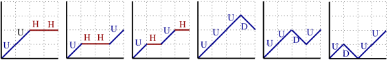
Figure 2: The set $\mathrm{GRP}(4,2)$ of Generalized Riordan paths from $(0,0)$ to $(4,2)$.

In our next lemma, we interpret Generalized Riordan paths as generalized Dyck paths with restrictions on the positions of its peaks. We denote paths with only Up and Down steps as UD paths. The following interpretation of Riordan paths is known (see OEIS) and we give a simple proof as we need a version for Generalized Riordan paths as well. Given a UD path $P$, a peak is a lattice point $(p,q)$ on $P$ such that an up-step ends at $(p,q)$ and a down-step starts at $(p,q)$.

Lemma 24

Let $n=2\ell$. For $0\leq k\leq\ell$, there is a bijection $f$ from $\mathrm{GRP}(\ell,\ell-k)$ to the set $\mathrm{NLP}(2\ell,2\ell-2k)$ of generalized Dyck paths from $(0,0)$ to $(2\ell,2\ell-2k)$ that have $2\ell-k$ Up steps, $k$ Down steps and have no peaks at any odd height. Thus, $\alpha_{2\ell,k,\ell}$ is the number of generalized Dyck paths from $(0,0)$ to $(2\ell,2\ell-2k)$ with $2\ell-k$ Up steps, $k$ Down steps, that have no peaks at any odd height.

Proof:   Let $P\in\mathrm{GRP}(\ell,\ell-k)$ with $P=a_{1},a_{2},\ldots,a_{\ell}$ be a Generalized Riordan path from $(0,0)$ to $(\ell,\ell-k)$ where $a_{i}=U/H/D$, depending on the type of the $i$-th step of $P$. Perform the following operations: change $U$ to $U,U$, change $D$ to $D,D$ and change $H$ to $D,U$. This will convert $P$ to $f(P)=Q=b_{1},b_{2},\ldots,b_{2\ell}$ where $Q$ is an UD path. We note the following properties of the bijection $f$.

(Property 1) $Q$ is a non negative path : As $P\in\mathrm{GRP}(\ell,\ell-k)$ and thus has no horizontal steps at height 0. Thus, changing a $H$ step in $P$ to $D,U$ in $f(P)$ will not make the path $f(P)$ go below height 0. Further, since $P$ is non negative, any $D$ step in $P$ is preceded by a $U$ step prior to it. This ensures that while changing $D$ in $P$ to $D,D$ in $f(P)$ we would have earlier changed a $U$ in $P$ to a $U,U$ in $f(P)$ and hence this change will also not make $f(P)$ go below height 0.

(Property 2) $Q$ has no peaks at any odd height : To see this, note that a peak will occur in $f(P)$ iff there is a consecutive $U,D$ pair. Suppose $(b_{i},b_{i+1})=(U,D)$, then it is easy to see that $i$ is even. As $i$ is even, this means that the height at which the peak occurs in $f(P)$ is also even. Thus any peak of $f(P)$ only occurs at an even height. The proof is now complete.  

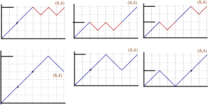
Figure 3: The generalized Dyck paths obtained under the bijection $f$ applied to paths in $\mathrm{GRP}(4,2)$.

Figure 3 shows the generalized Dyck paths output by the bijection $f$ described in Lemma 24 on paths $P\in\mathrm{GRP}(4,2)$. Note that Lemma 24 gives an interpretation for $\alpha_{2\ell,k,\ell}$, that is for entries in the last row when $n=2\ell$. Using this as a building block, we give another expression for $\alpha_{2\ell,k,i}$ in terms of $\alpha_{2m,k,m}$. This will enable us to give an interpretation for $\alpha_{2\ell,k,i}$.

Lemma 25

Let $n=2\ell$ and let $0\leq k,i\leq\ell$. Then,

$$\alpha_{2\ell,k,i}=\sum_{t=0}^{\ell-i}\binom{\ell-i}{t}\alpha_{2\ell-2t,k-t,\ell-t}.$$

Proof:   By Lemma 19, $\alpha_{2\ell,k,i}$ is the difference of succesive coefficients from the polynomial $p_{2\ell,i}(x)$. Set $b=1+x+x^{2}$. Then, for $k\geq 0$, we clearly have $p_{2k,k}(x)=b^{k}$. It is further clear that

$$p_{2\ell,i}(x) = (x+b)^{\ell-i}p_{2i,i}(x)=(x+b)^{\ell-i}b^{i}$$

$$= \sum_{t=0}^{\ell-i}\binom{\ell-i}{t}x^{t}b^{\ell-t}=\sum_{t=0}^{\ell-i}\binom{\ell-i}{t}x^{t}p_{2\ell-2t,\ell-t}(x)$$

As taking the difference of successive coefficients is a linear operator, we get the desired equation, completing the proof.  

Example 26

We illustrate Lemma 25 by getting the last column of the table when $n=8$. The following data can be easily verified.

$\ell$	0	1	2	3	4
$\alpha_{2\ell,\ell,\ell}$	1	0	1	1	3

From the table for $n=8$ in Example 5, one can easily verify the construction of the entries in the last column using the elements $\alpha_{2\ell,\ell,\ell}$ as follows.

$\alpha_{8,4,3}$	$=$	$4$	$=$	$\alpha_{8,4,4}+\alpha_{6,3,3},$
$\alpha_{8,4,2}$	$=$	$6$	$=$	$\alpha_{8,4,4}+2\alpha_{6,3,3}+\alpha_{4,2,2},$
$\alpha_{8,4,1}$	$=$	$9$	$=$	$\alpha_{8,4,4}+3\alpha_{6,3,3}+3\alpha_{4,2,2}+\alpha_{2,1,1},$
$\alpha_{8,4,0}$	$=$	$14$	$=$	$\alpha_{8,4,4}+4\alpha_{6,3,3}+6\alpha_{4,2,2}+4\alpha_{2,1,1}+\alpha_{0,0,0}.$

Using Lemma 25, we give an interpretation for the numbers $\alpha_{2\ell,k,i}$ when $i<\ell$. It will again be the the cardinality of a set of generalized Dyck paths with odd peaks occurring at restricted positions. All our generalized Dyck paths will be from $(0,0)$ to $(2\ell,2\ell-2k)$. Divide the $2\ell$ steps on the $x$-axis into $\ell$ intervals of length 2 each. Thus, we have intervals $s_{1}=(0,2)$, $s_{2}=(2,4),\ldots,s_{\ell}=(2\ell-2,2\ell)$. For $0\leq i\leq\ell$, define the sets $D_{i}=\{1,2,\ldots,i\}$. Thus $D_{0}=\emptyset$, $D_{1}=\{1\},D_{2}=\{1,2\}$ and so on. We will permit peaks to have an odd height at a point $(x,y)$ where $x\in D_{i}$.

Lemma 27

With the notation described above, $\alpha_{2\ell,k,i}$ is the cardinality of the set of generalized Dyck paths from $(0,0)$ to $(2\ell,2\ell-2k)$ with $2\ell-k$ Up steps, $k$ Down steps and odd peaks contained in the set $D_{\ell-i}$.

Proof:   Our proof is inspired by the proof of Lemma 25. We construct generalized Dyck paths with peaks at odd height in the set $D_{\ell-i}$ as follows. If there are peaks at odd heights, then as done in the proof of Lemma 24, it is clear that any such peak will occur at position $(x,y)$ where both $x,y$ are odd positive integers. Thus, such an odd peak causing “$U,D$” pair of steps has to be in positions indexed by $s_{d}$ for some $d\in\{1,2,\ldots,\ell\}$.

We claim that the number of generalized Dyck paths with $t$ odd height peaks in the set $D_{\ell-i}$ is $\binom{\ell-i}{t}\alpha_{2\ell-2t,k-t,\ell-t}$. If such a path $P$ is written as a string of $U,D$’s, any peak will have a consecutive “$U,D$” substring. Note that if $P$ has $t$ peaks at odd heights, then removing the $t$ “$U,D$” pairs will give a generalized Dyck path $Q$ of length $2\ell-2t$ with no change in the final height of the path (thus having $2\ell-k-t$ Up and $k-t$ Down steps) and with $t$ fewer $U$ steps and $t$ fewer $D$ steps. Further, $Q$ has no odd peaks. This argument goes both ways.

Given a generalized Dyck path $Q$ with a total of $2\ell-2t$ steps from $(0,0)$ to $(2\ell-2t,2\ell-2k)$ that has $2\ell-k-t$ Up steps and $k-t$ Down steps with no odd peaks, one can choose a subset $T$ of size $t$ from $D_{\ell-i}$ in $\binom{\ell-i}{t}$ ways and insert a “$U,D$” pair at position $s_{d}$ for $d\in T$. This completes the proof.  

Example 28

We illustrate the bijection described in Lemma 27 to get $\alpha_{8,4,0}$. We thus need Dyck paths from $(0,0)$ to $(8,0)$. Since we do not change the height, our building blocks are Dyck paths without peaks at odd heights from $(0,0)$ to $(2m,0)$ for non negative integers $m$. These are given in Figure 4 with different colours for added clarity. The set of paths formed is given in Figure 5 where the same colours are used and odd peak causing “U,D” pairs are drawn using dotted lines.

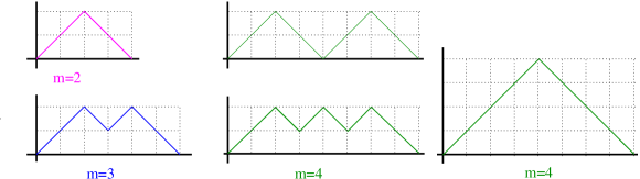
Figure 4: Up down paths with no peaks at an odd height.

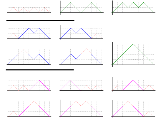
Figure 5: $\alpha_{8,4,0}$ counts all $14$ Catalan paths of semi-length $4$ that have peaks at odd heights in $D_{4}$.

Remark 29

Note that when $i=\ell$, Lemma 27 gives Lemma 24. Further, $\alpha_{2\ell,k,i}$ is a term that occurs in the normalized immanant computation of the partition $TwoRow_{k}$. Thus, when $\alpha_{n,k,i}$ is viewed as the cardinality of a restricted set of generalized Dyck paths as given in Lemma 27, the second parameter $k$ in the subscript of $\alpha_{2\ell,k,i}$ is the number of Down steps while the first parameter is the total number of steps in the generalized Dyck path.

Recall that $\alpha_{2\ell,\ell,0}=C_{\ell}$, the $\ell$-th Catalan number and as $\alpha_{2\ell-2t,\ell-t,\ell-t}=R_{\ell-t}$, where $R_{\ell}$ is the $\ell$-th Riordan number. When $n=2\ell,k=\ell$ and $i=0$, Lemma 25 gives us the known fact that $C_{\ell}=\sum_{t=0}^{\ell}\binom{\ell}{t}R_{\ell-t}$.

5.2 When $n=2\ell+1$ is odd

When $n=2\ell+1$, we use Lemma 4 which states that $\alpha_{2\ell+1,k,i}=\alpha_{2\ell,k,i}+\alpha_{2\ell,k-1,i}$. By Remark 29, $\alpha_{2\ell,k,i}$ and $\alpha_{2\ell,k-1,i}$ are the cardinalities of non negative UD paths where the first parameter $2\ell$ is the total number of steps while the second parameter $k$ is the number of Down steps. Further, these have odd height peaks in the set $D_{\ell-i}$.

The same interpretation works when $n=2\ell+1$. Consider non negative UD paths with $2\ell+1$ steps containing $k$ Down steps, which have one more Up step as compared to paths counted by the set with cardinality $\alpha_{2\ell,k,i}$. It is simple to see that there is a bijection between a non negative UD path $P$ counted by $\alpha_{2\ell,k,i}$ and the path $P^{\prime}=P,U$ where we append an Up step at the end of $P$. That is, if the last step of a path counted by $\alpha_{2\ell+1,k,i}$ is an Up step, then by deleting it, we get an non negative UD path counted by $\alpha_{2\ell,k,i}$. However, if the last step is a Down step, then after deletion of this, we get a non negative path counted by the $\alpha_{2\ell,k-1,i}$. We only need to check that appending a Down step at the end does not create a valley at an odd height. But this follows from the fact that a path with $2\ell$ steps and $k-1$ Down steps ends at a point $(2\ell,2\ell-2k+2)$ and so ends at a point with even $y$ co-ordinate. Adding a Down step to such a path may create a peak but only at an even height. Thus, the set of odd height peaks after addition of a Down step at the end does not change. Thus we get the following counterpart of Lemma 27.

Lemma 30

With the notation described above, $\alpha_{2\ell+1,k,i}$ is the cardinality of the set of non negative UD paths from $(0,0)$ to $(2\ell+1,2\ell-2k+1)$ with $2\ell-k+1$ Up steps, $k$ Down steps and odd peaks contained in the set $D_{\ell-i}$.

5.3 Probabilistic Interpretation of Lemma 16

From Lemma 27 and Lemma 30, we get the following probabilistic interpretation of Lemma 16 whose straightforward proof we omit.

Lemma 31

Fix a positive integer $n$ and $i\leq\lfloor(n-1)/2\rfloor$. Then, the probability of a non negative UD path with $n$ total steps and with odd height peaks contained in the set $D_{\lfloor n/2\rfloor-i}$ decreases as the number $k$ of Down steps increases.

Recall that Remark 20 gives a bijection between non negative UD paths with $n$ steps and with $k$ down steps and Standard Young Tableaux of shape $n-k,k$ (denoted $\mathsf{SYT}(n-k,k)$), we can recast Lemma 31 in terms of SYTs. We translate the notion of peaks at odd heights to tableaux. For $T\in\mathsf{SYT}(n-k,k)$ define position $i$ to be a peak if $i$ appears in the first row and $i+1$ appears in the second row. This is precisely saying that $i\in\mathrm{DES}(T)$ where $\mathrm{DES}(T)$ is the descent set of $T$, which is a well studied statistic (see the book by Stanley [15, Chapter 7]). For a descent $i$, to get the height of its peak under this mapping, consider $T_{|i}$, the restriction of $T$ to the entries $\{1,2,\ldots,i\}$. Note that $T_{|i}$ is also an SYT. Let $T_{|i}=a_{i},b_{i}$ where $a_{i}$ and $b_{i}$ are the number of elements in the first and second row of $T_{|i}$ respectively. Define $\mathrm{RowDiff}(T_{|i})=a_{i}-b_{i}$ to be the difference between the number of elements in the first row and the number of elements in the second row of $T_{|i}$. Define an descent $i\in T$ to have even (or odd) height if $\mathrm{RowDiff}(T_{|i})$ is even (or odd respectively). With these definitions, recalling the set $D_{\ell-i}$, we can give the SYT version of Lemma 31.

Lemma 32

Fix a positive integer $n$ and let $i\leq\lfloor(n-1)/2\rfloor$. Then, the probability that an SYT of shape $n-k,k$ has all its descents with odd height in $D_{\lfloor n/2\rfloor-i}$ decreases as the number $k$ increases (and hence the shape of $T$ changes).

By running the arguments backward, it is clear that an alternate proof of Lemma 32 will give us an alternate proof of Theorem 2. Thus, it would be interesting to get an alternate proof of Lemma 32.

References

- [1] Bapat, R. B. Resistance matrix and -laplacian of a unicyclic graph. In Ramanujan Mathematical Society Lecture Notes Series, 7, Proceedings of ICDM 2006, Ed. R. Balakrishnan and C.E. Veni Madhavan (2008), pp. 63–72.
- [2] Bapat, R. B., Lal, A. K., and Pati, S. A -analogue of the distance matrix of a tree. Linear Algebra and its Applications 416 (2006), 799–814.
- [3] Bapat, R. B., and Sivasubramanian, S. The Third Immanant of q-Laplacian Matrices of Trees and Laplacians of Regular Graphs. Springer India, 2013, pp. 33–40.
- [4] Bass, H. The Ihara-Selberg Zeta Function of a Tree Lattice. International Journal of Math. 3 (1992), 717–797.
- [5] Bessenrodt, C. Coincidences between Characters to Hook Partitions and 2-Part Partitions on Families arising from 2-Regular Classes. Electronic Journal of Combinatorics 24 (3) (2017).
- [6] Callan, D. Riordan Numbers Are Differences of Trinomial Coefficients. Available at http://pages.stat.wisc.edu/callan/notes/riordan/riordan.pdf (2006).
- [7] Chan, O., and Lam, T. K. Binomial Coefficients and Characters of the Symmetric Group. Technical Report 693 (1996), National Univ of Singapore.
- [8] Csikvári, P. On a Poset of Trees. Combinatorica 30 (2) (2010), 125–137.
- [9] Csikvári, P. On a Poset of Trees II. Journal of Graph Theory 74 (2013), 81–103.
- [10] Foata, D., and Zeilberger, D. Combinatorial Proofs of Bass’s Evaluations of the Ihara-Selberg Zeta function of a Graph. Transactions of the AMS 351 (1999), 2257–2274.
- [11] Nagar, M. K., and Sivasubramanian, S. Hook immanantal and Hadamard inequalities for -Laplacians of trees. Linear Algebra and its Applications 523 (2017), 131–151.
- [12] Nagar, M. K., and Sivasubramanian, S. Laplacian immanantal polynomials and the gts poset on trees. Linear Algebra and Applications 561 (2019), 1–23.
- [13] Sagan, B. E. The Symmetric Group: Representations, Combinatorial Algorithms, and Symmetric Functions, 2nd ed. Springer Verlag, 2001.
- [14] Schur, I. Über endliche Gruppen und Hermitesche Formen. Math. Z. 1 (1918), 184–207.
- [15] Stanley, R. P. Enumerative Combinatorics, vol 2. Cambridge University Press, 2001.
- [16] Zeilberger, D., and Regev, A. Surprising Relations Between Sums-Of-Squares of Characters of the Symmetric Group Over Two-Rowed Shapes and Over Hook Shapes. Séminaire Lotharingien de Combinatoire 75, Article B75c (2016).