Laplacian Immanantal Polynomials of a Bipartite Graph and Graph Shift Operation

Abstract.

Let $G$ be a bipartite graph on $n$ vertices with the Laplacian matrix $L_{G}$. When $G$ is a tree, inequalities involving coefficients of immanantal polynomials of $L_{G}$ are known as we go up $\mathrm{GTS}_{n}$ poset of unlabelled trees with $n$ vertices. We extend $\mathrm{GTS}$ operation on a tree to an arbitrary graph, we call it generalized graph shift (hencefourth $\mathrm{GGS}$) operation. Using $\mathrm{GGS}$ operation, we generalize these known inequalities associated with trees to bipartite graphs. Using vertex orientations of $G$, we give a combinatorial interpretation for each coefficient of the Laplacian immanantal polynomial of $G$ which is used to prove counter parts of Schur theorem and Lieb’s conjecture for these coefficients. We define $\mathrm{GGS}_{n}$ poset on $\Omega_{C_{k}}^{v}(n)$, the set of unlabelled unicyclic graphs with $n$ vertices where each vertex of the cycle $C_{k}$ has degree $2$ except one vertex $v$. Using $\mathrm{GGS}_{n}$ poset on $\Omega_{C_{2k}}^{v}(n)$, we solves an extreme value problem of finding the max-min pair in $\Omega_{C_{2k}}^{v}(n)$ for each coefficient of the generalized Laplacian polynomials. At the end of this paper, we also discuss the monotonicity of the spectral radius and the Wiener index of an unicyclic graph when we go up along $\mathrm{GGS}_{n}$ poset of $\Omega_{C_{k}}^{v}(n)$.

KEYWORDS : $\mathrm{GTS}$ poset, bipartite graphs, $\mathrm{GGS}$ operation, vertex orientation, immanantal polynomial.
AMS CLASSIFICATION : 05C05 06A06 15A15

1. Introduction

For a positive integer $n$, let $\mathfrak{S}_{n}$ denote the symmetric group on $[n]=\{1,2,\ldots,n\}$. A partition $\lambda$ of $n$ is denoted by $\lambda\vdash n$ and it is written using the exponential notation with multiplicities of parts written as exponents. Thus, if $i$ appears $n_{i}$ times in $\lambda$ then $\lambda=1^{n_{1}}2^{n_{2}}3^{n_{3}}\ldots$ and $n_{1}+2n_{2}+3n_{3}+\cdots=n.$ For $\lambda\vdash n$, let $\chi_{\lambda}$ denote the corresponding irreducible character of $\mathfrak{S}_{n}$ over $\mathbb{C}$, the set of complex numbers, (see the textbook by Sagan [17] as a reference for the theory of characters of $\mathfrak{S}_{n}$). Let $A=(a_{i,j})\in{\mathbb{M}}_{n}(\mathbb{C})$, where ${\mathbb{M}}_{n}(\mathbb{C})$ represents the set of all $n\times n$ matrices with complex entries. Then, the normalized immanant function of $A$ associated with $\lambda\vdash n$, denoted $\overline{\mathrm{imm}}_{\lambda}(\cdot)$ is defined as

(1) $$\overline{\mathrm{imm}}_{\lambda}(A)=\dfrac{1}{\chi_{\lambda}(\mathsf{id})}\sum_{\psi\in\mathfrak{S}_{n}}\chi_{\lambda}(\psi)\prod_{i=1}^{n}a_{i,\psi(i)},$$

where $\chi_{\lambda}(\mathsf{id})$ is the dimension of the irreducible representation indexed by $\lambda$. The expression $\chi_{\lambda}(\mathsf{id})\overline{\mathrm{imm}}_{\lambda}(A)$ from Equation (1) is called the immanant function of $A$ and it is denoted as $\mathrm{imm}_{\lambda}(A)$. As $\chi_{1^{n}}(\mathsf{id})=1=\chi_{n}(\mathsf{id})$, we see that $\overline{\mathrm{imm}}_{1^{n}}(A)=\det(A)$ and $\overline{\mathrm{imm}}_{n}(A)=\mathrm{perm}(A)$, where $\det(A)$ and $\mathrm{perm}(A)$ are the determinant and the permanent of $A$, respectively.

Let ${\mathbb{H}}_{n}(\mathbb{C})$ be the set of all $n\times n$ positive semidefinite Hermitian matrix over $\mathbb{C}$. Then, Schur in [19] showed that $\det(A)=\min\ \{\overline{\mathrm{imm}}_{\lambda}(A):\lambda\vdash n\}$ for all $A\in{\mathbb{H}}_{n}(\mathbb{C})$. Towards getting the maximum element in this set, a popular conjecture known as the “permanental dominance conjecture” was given by Lieb in [10]. It states that $\mathrm{perm}(A)=\max\ \{\overline{\mathrm{imm}}_{\lambda}(A):\lambda\vdash n\}$ for all $A\in{\mathbb{H}}_{n}(\mathbb{C})$. This is still open. In this paper, we give a proof of this conjecture for the Laplacian matrix of a bipartite graph, see Theorem 8.

For a simple graph $G$ with vertex set $[n]$, its Laplacian matrix $L_{G}$ is defined by $L_{G}=D-A(G)$, where $A(G)$ is the adjacency matrix of $G$ and $D$ is the diagonal matrix with vertex degrees on the main diagonal. Indexed by $\lambda\vdash n$, the Laplacian immanantal polynomial of $G$, denoted $\phi_{\lambda}(L_{G},x)$ is defined as $\phi_{\lambda}(L_{G},x)=\mathrm{imm}_{\lambda}(xI-L_{G})$. For $0\leq r\leq n$, let $b_{\lambda,r}(L_{G})$ be the coefficient of $(-1)^{r}x^{n-r}$ in $\phi_{\lambda}(L_{G},x)$, that is

(2) $$\phi_{\lambda}(L_{G},x)=\sum_{r=0}^{n}(-1)^{r}b_{\lambda,r}(L_{G})x^{n-r}$$

Let $T$ be a tree on $n$ vertices with Laplacian matrix $L_{T}$. Let $S_{n}$ and $P_{n}$ be the star tree and the path tree on $n$ vertices respectively. When $\lambda=1^{n}\vdash n$, Gutman and Povlovic in [7] conjectured the following inequality which was proved by Gutman and Zhou [8] and independently by Mohar [12]

(3) $$b_{1^{n},r}(L_{S_{n}})\leq b_{1^{n},r}(L_{T})\leq b_{1^{n},r}(L_{P_{n}})\mbox{ for }r=0,1,2,\ldots,n.$$

The heart of this paper is the $\mathrm{GGS}$ (generalized graph shift) operation which is used to study the monotonicity results of some graph-theoretical parameters. Some of them are discussed here, for instances, the spectral radius, Wiener index and coefficients of the Laplacian immanantal polynomials (see Theorems 2 and 18 and Corollary 21).

Kelmans [9] was the first who studied an operation on graphs called Kelmans transformation, see Definition 1. This transformation increases the spectral radius and decreases the number of spanning trees (for more details see Brown, Colbourn and Devitt [1] and Satyanarayana, Schoppman and Suffel [18]. Similar type of transformation which is called generalized tree shift (abbreviated as $\mathrm{GTS}$ henceforth) operation was defined by Csikvári in [5] to construct a poset called $\mathrm{GTS}_{n}$ on the set of unlabelled trees with $n$ vertices, see Definition 2. Later, this $\mathrm{GTS}$ operation was studied in [6, 13, 15, 16] in order to discuss monotonicity properties of some graph-theoretical parameters (see Table 1). Csikvári showed that the star tree $S_{n}$ and the path tree $P_{n}$ are the only maximal and minimal elements of $\mathrm{GTS}_{n}$ respectively. Thus for all monotonicity results on $\mathrm{GTS}_{n}$, the max-min pair is either $(P_{n},S_{n})$ or $(S_{n},P_{n})$ among all trees with $n$ vertices. Among other results, he proved that going up along $\mathrm{GTS}_{n}$ decreases each coefficient of the characteristic polynomial of $L_{T}$ in absolute value and hence the max-min pair for this algebraic parameter is $(P_{n},S_{n})$. Thus Csikvári’s result is more general than the inequality given in (3). Using $\mathrm{GTS}_{n}$ the following stronger inequality involving the Laplacian immanantal polynomial of a tree than the one mentioned above, appeared in Nagar and Sivasubramanian [15, Theorem 1].

Theorem 1 (Nagar and Sivasubramanian).

Let $T$ be a tree on $n$ vertices. Then for all $\lambda\vdash n$, going up on $\mathrm{GTS}_{n}$ decreases each coefficient in absolute value, that is $b_{\lambda,r}(L_{T})$ of the Laplacian immanantal polynomial of $T$ indexed by $\lambda$.

Csikvári’s $\mathrm{GTS}_{n}$ poset and the above results motivated us to extend the notion of generalized tree shift operation on trees to arbitrary graphs. We will call this new operation as the generalized graph shift (abbreviated as $\mathrm{GGS}$ henceforth), see Definition 3. The $\mathrm{GGS}$ operation gives us a poset on the set of unlabelled unicylic graphs with certain conditions. The $\mathrm{GGS}$ poset and the following theorem which is our main result, are used to solve an extreme value problem of finding the max-min pair in set of unlabelled unicyclic graphs (see Theorem 18 and Corollary 21).

Theorem 2.

Let $G$ be a bipartite graph on $n$ vertices and let $L_{G}$ be its Laplacian matrix. Then for all $\lambda\vdash n$ and for all $r\geq 0$, each coefficient $b_{\lambda,r}(L_{G})$ given in (2) is a non-negative integer and the $\mathrm{GGS}$ operation decreases each $b_{\lambda,r}(L_{G})$.

Let $G$ be a bipartite graph on $n$ vertices with the Laplacian matrix $L_{G}$. Using Theorem 2, we obtain several corollaries involving the constant term of the immanantal polynomials of $L_{G}$.

The layout of this paper is the following: The next section introduces the concepts of Kelmans transformation, the generalized tree shift poset and it’s generalized version, the $\mathrm{GGS}$ operation on arbitrary graphs. In Section 3, a very basic facts and an elementary relationship between $\mathrm{imm}_{\lambda}(L_{G})$ and the enumerations of vertex orientations in a bipartite graph $G$ are given. Lieb’s conjecture for the Laplacian immanants of a $G$ is also proved. These results are generalized to each coefficient of the Laplacian immanantal polynomial of a bipartite graph in Section 4. In Section 5, we prove Theorem 2 which can be thought as a result involving coefficients of the generalized matrix polynomial indexed by the Schur symmetric function, since each irreducible character of $\mathfrak{S}_{n}$ is the inverse image of the Frobenius characteristic map of the Schur symmetric function (see Sagan [17] for more details). Further, Theorem 2 is extended to the generalized matrix polynomial of $L_{G}$ associated with the elementary, power sum and complete homogeneous symmetric functions in Section 6. In the last section, using $\mathrm{GGS}$ operation, the monotonicity property of the spectral radius and Wiener index of a graph are discussed.

2. Graph operations

Throughout this paper, our graphs are simple and connected with vertex set $[n]$. The contents of this section, may be conveniently presented into two parts separately introduce the notion of Kelmans transformation, $\mathrm{GTS}_{n}$ poset and it’s generalized version for arbitrary graphs. These graph operations are main tools to discuss monotonicity results involving some algebraic and topological parameters of a graph. Using $\mathrm{GTS}$ operation and generalized graph shift, some of them are determined and are mentioned in Table 1, Theorem 18 and Corollary 21.

2.1. Kelmans transformation and $\mathrm{GTS}_{n}$ poset

Towards defining the Kelmans transformation, we need the following terminology and notations. For a given vertex $v$ in a graph $G$, define $N[v]$ to be the set of neighbours of $v$ containing $v$. Define $N(v):=N[v]\setminus\{v\}$, that is, $N[v]$ is a disjoint union of $v$ and $N(v)$. We begin with the following definition of Kelmans transformation.

Definition 1.

Let $G_{1}$ be a graph with $n$ vertices and let $x$ and $y$ be two arbitrary vertices of $G_{1}$. We construct a graph $G_{2}$ by erasing all edges between $x$ and $N(x)\setminus N[y]$ and add edges between $y$ and $N(x)\setminus N[y]$. This operation is called Kelmans transformation. We note that the number of edges in the obtained graph $G_{2}$ equals the number of edges in $G_{1}$.

Kelmans transformation can be applied to any graph, but if we consider it as a transformation on trees to get a connected graph we have to make a restriction on vertices $x$ and $y$ in $G_{1}$. Namely they should have distance at most $2$ in order to obtain a connected graph $G_{2}$ as a result. To handle this problem Csikvári [5] put some restrictions on $x$ and $y$ to define the generalized tree shift operation on trees. From [5], we recall his definition of $\mathrm{GTS}_{n}$ poset on the set of unlabelled trees with $n$ vertices.

Definition 2.

Let $T_{1}$ be a tree with $n$ vertices. Assume that $1$ and $k$ are two vertices of $T_{1}$ such that the interior vertices (if they exist) on the unique path $P_{1,k}$ between $1$ and $k$, have degree 2. Let $k-1$ be the neighbour of $k$ on $P_{1,k}$. Construct a new tree $T_{2}$ by moving all neighbours of $k$ except $k-1$ to the vertex $1$. This operation is called the generalized tree shift. Here, we say $T_{2}$ is obtained from $T_{1}$ using $\mathrm{GTS}$ operation. This is illustrated in Figure 1. The generalized tree shift operation gives us a partial order denoted as “$\leq_{\mathrm{GTS}_{n}}$” on the set of unlabelled trees on $n$ vertices.

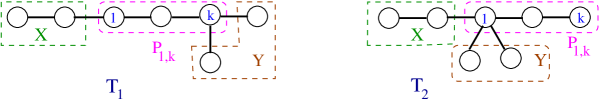
Figure 1. Two trees with $T_{1}\leq_{\mathrm{GTS}_{n}}T_{2}$.

If $T_{1}\leq_{\mathrm{GTS}_{n}}T_{2}$, we say tree $T_{1}$ is below $T_{2}$ or $T_{2}$ is above $T_{1}$. When $n=6$, we refer the reader to Csikvári [5] for the Hasse diagram of $\mathrm{GTS}_{6}$. Among other results he proved the following important result which gives the max-min pair for a monotonicity result on $\mathrm{GTS}_{n}$ poset.

Lemma 3 (Csikvári).

Among trees, the star graph $S_{n}$ and the path graph $P_{n}$ on $n$ vertices are the only maximal and the minimal elements of $\mathrm{GTS}_{n}$ respectively.

Thus, for all monotonicity results on $\mathrm{GTS}_{n}$, the max-min pair among all unlabelled trees on $n$ vertices is either $(P_{n},S_{n})$ or $(S_{n},P_{n})$. For some well known monotonicity results, the max-min pair in the set of trees with $n$ vertices, are given in Table 1. When we go up along $\mathrm{GTS}_{n}$, upward ($\uparrow$) and downward ($\downarrow$) arrows show graph-theoretical parameters which are increasing and decreasing respectively. For instance, in [6] authors showed that the largest eigenvalues of both the matrices, adjacency $A(T)$ and the Laplacian $L_{T}$ increase and hence the max-min pairs for these spectral properties are $(S_{n},P_{n})$. Later in [13] authors generalized these results to the $q$-Laplacian and $q,t$-Laplacian matrix for all $q,t\in\mathbb{R}_{\geq 0}$, the set of non-negative reals. They also proved results involving exponential distance matrix and determined the max-min pair for the largest and the smallest eigenvalues among the set of unlabelled trees with $n$ vertices.

Graph-theoretical parameter	Monotonicity	Max-Min pair
Number of closed walks of a fixed length $\ell$ [5]	$\uparrow$	$(S_{n},P_{n})$
Estrada index [5]	$\uparrow$	$(S_{n},P_{n})$
Wiener index [5]	$\downarrow$	$(P_{n},S_{n})$
Algebraic connectivity [6]	$\uparrow$	$(S_{n},P_{n})$
The largest eigenvalue of adjacency and the Laplacian [6]	$\uparrow$	$(S_{n},P_{n})$
Coefficients of matching polynomial [6]	$\downarrow$	$(P_{n},S_{n})$
Coefficients of the Laplacian immanantal polynomial [15]	$\downarrow$	$(P_{n},S_{n})$

Table 1. Monotonicity of graph theoretical parameters when we go up along $\mathrm{GTS}_{n}$.

2.2. Generalized graph shift

Inspired by Kelmans transformation and $\mathrm{GTS}_{n}$ poset, an identical definition of the generalized graph shift operation on a graph $G$ is given in this subsection. To define $\mathrm{GGS}$ operation on $G$, some restrictions are used on the chosen vertices $x$ and $y$ of $G$ in Kelmans transformation defined above but the $\mathrm{GTS}$ operation on a tree is generalized for an arbitrary graph.

Definition 3.

Let $G_{1}$ be an arbitrary graph with $n$ vertices. Let $1$ and $k$ be two vertices in $G_{1}$ connected via a path say $P_{1,k}$ from $1$ to $k$ such that

1. each interior vertices (if they exist) on $P_{1,k}$ have degree 2 and

2. both the vertices $1$ and $k$ are not contained in one cycle of $G_{1}$.

Thus $k$ has a unique neighbor on $P_{1,k}$, let it be $k-1$. Construct a graph $G_{2}$ by moving all neighbours of $k$ except $k-1$ to the vertex $1$. Thus, all neighbors of $k$ which do not lie on the path $P_{1,k}$ have become neighbors of $1$ in $G_{2}$. This operation is called the generalized graph shift (henceforth $\mathrm{GGS}$), denoted $G_{2}=\mathrm{GGS}(G_{1})$. Note that the $\mathrm{GTS}$ operation is a special case of $\mathrm{GGS}$ construction when $G_{1}$ is a tree. For the sake of clarity $\mathrm{GGS}$ operation is illustrated in Figure 2.

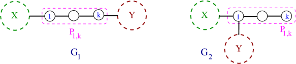
Figure 2. Two graphs $G_{1}$ and $G_{2}$ such that $G_{2}=\mathrm{GGS}(G_{1})$.

In the above definition, vertices $1$ and $k$ are called the recipient and the donor, respectively. Here we note that if the role of the recipient and donor in $G_{1}$ are exchanged then the obtained graph in $\mathrm{GGS}$ operation is isomorphic to $G_{2}$. It is easy to check that $\mathrm{GGS}$ increases the number of leaf vertices. In fact the number of leaves in $G_{2}$ is one more than the number of leaves in $G_{1}$ if and only if both $1$ and $k$ are not leaves in $G_{1}$.

2.3. Applications of $\mathrm{GGS}$ operation

For two positive integers $n$ and $k$ with $n>k\geq 3$, let $\Omega_{C_{k}}^{v}(n)$ be the set of all unlabelled unicyclic graphs with $n$ vertices where the length of the unique cycle $C_{k}$ is $k$ and the degree of each vertex in $C_{k}$ is $2$ except one vertex $v\in C_{k}$. We define an order relation, denoted “$\leq_{\mathrm{GGS}_{n}}$” on $\Omega_{C_{k}}^{v}(n)$ as follows: If $G_{1},G_{2}\in\Omega_{C_{k}}^{v}(n)$ and $G_{2}$ is obtained from $G_{1}$ using some number of $\mathrm{GGS}$ operations on $G_{1}$ then $G_{1}\leq_{\mathrm{GGS}_{n}}G_{2}$. It is easy to check that the relation $\leq_{\mathrm{GGS}_{n}}$ is a partial order on the set $\Omega_{C_{k}}^{v}(n)$. For the sake of clarity, when $n=8$ and $k=4$ the Hasse diagram of $\mathrm{GGS}_{8}$ poset on $\Omega_{C_{4}}^{v}(8)$ is given in Figure 3.

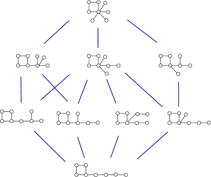
Figure 3. The Hasse diagram of $\mathrm{GGS}$ poset on the set $\Omega_{C_{4}}^{v}(8)$.

For a fixed positive integer $k\geq 3$, let $C_{k}$ be the cycle on $k$ vertices. Let $S_{n-k+1}$ be the star graph on $n-k+1$ vertices such that vertex $v_{1}\in S_{n-k+1}$ has degree $n-k$. Construct a new graph $G_{S_{n-k+1}}$ by moving all neighbours of $v_{1}$ to a vertex (say $v$) of $C_{k}$ and deleting $v_{1}$. This operation of joining $S_{n-k+1}$ to $C_{k}$ is denoted as $S_{n-k+1}|v_{1}:C_{k}|v$. Thus $G_{S_{n-k+1}}=S_{n-k+1}|v_{1}:C_{k}|v$ is an unicyclic graph with $n$ vertices. Let $P_{n-k+1}$ be the path graph on $n-k+1$ vertices such that $v_{2}\in P_{n-k+1}$ is a leaf vertex. Analogously, define $G_{P_{n-k+1}}:=P_{n-k+1}|v_{2}:C_{k}|v$ as an unicyclic graph with $n$ vertices having cycle $C_{k}$ of length $k$ and each vertex in $C_{k}$ has degree $2$ except the vertex $v$ which has degree $3$ in $G_{P_{n-k+1}}$. It is easy to check that $G_{S_{n-k+1}},G_{P_{n-k+1}}\in\Omega_{C_{k}}^{v}(n)$. Since the proof of the following lemma is identical to the proof of Lemma 3, we omit it and merely state the result.

Lemma 4.

Let $G_{S_{n-k+1}}$ and $G_{P_{n-k+1}}$ be the unicyclic graphs defined in the above paragraph. Then $G_{S_{n-k+1}}$ and $G_{P_{n-k+1}}$ are the only maximal and the minimal elements of $\mathrm{GGS}_{n}$ poset on $\Omega_{C_{k}}^{v}(n)$ respectively.

The above lemma is illustrated in Figure 3, the Hasse diagram of $\mathrm{GGS}_{8}$ poset on the subset $\Omega_{C_{4}}^{v}(8)$ of unlabelled unicyclic graphs with $8$ vertices. Thus for all monotonicity results on the $\mathrm{GGS}_{n}$ poset of $\Omega_{C_{k}}^{v}(n)$, the max-min pair is either $(G_{S_{n-k+1}},G_{P_{n-k+1}})$ or $(G_{P_{n-k+1}},G_{S_{n-k+1}})$. When we restrict $\mathrm{GGS}$ operation to the set of bipartite graphs for calculating the Laplacian immanantal polynomial, Theorem 2 determines the max-min pair in the set $\Omega_{C_{2k}}^{v}(n)$ for the each coefficient $b_{\lambda,r}(L_{G})$ where $\lambda\vdash n$, $k\geq 2$ and $r=0,1,\ldots,n$.

Remark 5.

In the above $\mathrm{GGS}_{n}$ poset on the set $\Omega_{C_{k}}^{v}(n)$, the cycle $C_{k}$ can be replaced by any connected graph to construct different poset on some subset of connected graphs. For instance, when $C_{4}$ is replaced by $P_{2}$ in Figure 3, we get the Hasse diagram of $\mathrm{GTS}_{6}$ given in Csikvári [5].

3. Vertex Orientations and Immanants of Bipartite Graphs

It is worth pointing out the notion of vertex orientation that has appeared in several context and having connections with the number of matchings, moments of vertices, coefficients of the Laplacian immanantal polynomial and Wiener index of a tree (for more details see [3, 4, 14, 15]). For convenience of the reader, we repeat some relevant material on vertex orientation from [3, 14, 15] without proof, thus making our exposition self contained. In this paper, enumeration of vertex orientations will be used to express each coefficient of the Laplacian immanantal polynomial of a bipartite graph as a sum of non-negative terms. From [3, 14] we recall the following definition of vertex orientation of a graph.

Definition 4.

Let $G$ be a graph with $n$ vertices. In a vertex orientation $O$ of $G$, we assign an arrow to each vertex $v\in G$ pointing away from $v$ along one of its incidence edges. If $\deg(v)$ denotes the degree of $v\in G$ then there are $\deg(v)$ choices of assigning an arrow to $v$ in $G$. Such an assignment of arrows to each vertex of $G$ is said to be a vertex orientation. Throughout this paper, $O(v)=u$ denotes the arrow of $v$ assigned on the edge $(v,u)$, away from $v$ and towards $u$. It is illustrated in Figure 4.

From the above definition of vertex orientation in a graph $G$, it is easy to check that each edge in $G$ can have atmost two arrows on it. Let $G$ be a bipartite graph with $n$ vertices and let $O$ be a vertex orientation in $G$. Since $G$ is a bipartite graph, no directed cycle with odd length can be possible in $O$. As done by Chan and Lam in [3], if in $O$, there are $n_{1}$ edges with one arrow on them, $n_{2}$ bidirected edges (with two arrows on them), $n_{4}$ directed $4$-cycles, $\ldots$, $n_{2k}$ directed $2k$-cycles for $k\geq 3$ then it is simple to check that $n_{1}+2n_{2}+4n_{4}+\cdots+2kn_{2k}+\cdots=n$ where $n_{1},n_{2},n_{4},\ldots,n_{2k},\ldots\in\mathbb{Z}_{\geq 0}$, the set of non-negative integers. Each orientation $O$ in a bipartite graph gives us a partition $\mu=(1^{n_{1}},2^{n_{2}},4^{n_{4}},\ldots)$ of $n$. Such an orientation $O$ in $G$ is said to be of type $\mu$ orientation. Let us define $\mathcal{O}_{\mu}^{G}$ to be the set of vertex orientations in $G$ of type $\mu$ and let $|\mathcal{O}_{\mu}^{G}|=a_{G}(\mu)$. Let $\mathcal{PO}_{G}(n)$ be the set of all possible partitions of $n$ obtained from the set of orientations in $G$. In Figure 4, three vertex orientations $O$, $P$ and $Q$ of a bipartite graph $G=P_{3}|1:C_{4}|1\in\Omega_{C_{4}}^{1}(6)$ are given. It is very easy to check that the types of $O$, $P$ and $Q$ are $(1^{2},2^{2})$, $(1^{2},4^{1})$ and $(2^{1},4^{1})$, respectively. In $O,P$ and $Q$, edges with two arrows and a 4-cycle are depicted with using brown and blue colours (can seen better on a color monitor), respectively.

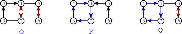
Figure 4. Three vertex orientations of $C_{4}|1:P_{3}|1$.

Let $P(n)$ be the set of all partitions of $n$. For $\lambda\vdash n$, let $\chi_{\lambda}$ denote the corresponding irreducible character of $\mathfrak{S}_{n}$. In this paper, $\chi_{\lambda}(\nu)$ will be denoted the character value $\chi_{\lambda}(\psi)$ evaluated at a permutation $\psi\in\mathfrak{S}_{n}$ with cycle type $\nu$. For $\nu,\mu\in P(n)$ with $\mu=(1^{n_{1}},2^{n_{2}},3^{n_{3}},\ldots,n^{n_{n}})$ and $\nu=(1^{m_{1}},2^{m_{2}},3^{m_{3}},\ldots,n^{m_{n}})$, we define $\binom{\mu}{\nu}=\binom{n_{2}}{m_{2}}\binom{n_{3}}{m_{3}}\cdots\binom{n_{n}}{m_{n}}$, where $\binom{n_{i}}{m_{i}}$ is the binomial coefficient and $\binom{n_{i}}{m_{i}}=0$ if $n_{i}<m_{i}$. For $\lambda,\mu\vdash n$, define $\alpha_{\lambda,\mu}$ as the following binomial weighted sum involving a character $\chi_{\lambda}$ of $\mathfrak{S}_{n}$ and binomial coefficients.

(4) $$\alpha_{\lambda,\mu}=\sum_{\nu\in P(n)}\chi_{\lambda}(\nu)\binom{\mu}{\nu}.$$

When $\mu=(1^{n_{1}},2^{n_{2}},4^{n_{4}},\ldots)$ with $n_{i}=0$ for all $i>2$, Chan and Lam [2] showed that $\alpha_{\lambda,\mu}$ is a non-negative integral multiple of $2^{n_{2}}$. In [3, Lemma 3.1], they also proved the following more general result which will be used to combinatorialise the coefficient $b_{\lambda,r}(L_{G})$ of Laplacian immanantal polynomial of the bipartite graph $G$.

Lemma 6 (Chan and Lam).

For all $\lambda,\mu\in P(n)$, the term $\alpha_{\lambda,\mu}$ defined in (4), is a non-negative integer.

Using enumeration of vertex orientations and Lemma 6, Chan and Lam in [3, page 5] proved the following result in order to determine the Laplacian immanants of a bipartite graph.

Lemma 7 (Chan and Lam).

Let $G$ be a bipartite graph on $n$ vertices with $L_{G}$ as its Laplacian matrix. Then for all $\lambda\vdash n$,

$$\mathrm{imm}_{\lambda}(L_{G})=\sum_{\mu\in\mathcal{PO}_{G}(n)}a_{G}(\mu)\sum_{\nu\in P(n)}\chi_{\lambda}(\nu)\binom{\mu}{\nu}=\sum_{\mu\in P(n)}a_{G}(\mu)\alpha_{\lambda,\mu},$$

where $a_{G}(\mu)$ is the number of vertex orientations of type $\mu$ in $G$.

From Section 1 we recall that the following result is the Lieb’s conjecture involving Laplacian immanants of a bipartite graph.

Theorem 8 (Lieb’s Conjecture for bipartite graphs).

Let $G$ be a bipartite graph with $n$ vertices and let $L_{G}$ be its Laplacian matrix. Then for all $\lambda\vdash n$, $\overline{\mathrm{imm}}_{\lambda}(L_{G})\leq\mathrm{perm}(L_{G}).$

Proof.

From Lemma 7, we have

$$\overline{\mathrm{imm}}_{\lambda}(L_{G})= \frac{\mathrm{imm}_{\lambda}(L_{G})}{\chi_{\lambda}(\mathsf{id})}=\sum_{\mu\in\mathcal{PO}_{G}(n)}a_{G}(\mu)\sum_{\nu\in P(n)}\frac{\chi_{\lambda}(\nu)}{\chi_{\lambda}(\mathsf{id})}\binom{\mu}{\nu}$$

$$\leq\sum_{\mu\in P(n)}a_{G}(\mu)\sum_{\nu\in P(n)}\left|\frac{\chi_{\lambda}(\nu)}{\chi_{\lambda}(\mathsf{id})}\right|\binom{\mu}{\nu}$$

$$\leq\sum_{\mu\in P(n)}a_{G}(\mu)\sum_{\nu\in P(n)}\binom{\mu}{\nu}=\mathrm{perm}(L_{G}).$$

The above identity follows from the fact that for each $\lambda\vdash n$ and for each permutation $\psi\in\mathfrak{S}_{n}$, we have $\left|\frac{\chi_{\lambda}(\psi)}{\chi_{\lambda}(\mathsf{id})}\right|\leq 1$. Hence the proof is complete. ∎

It is well known that for a bipartite graph $G$ with $n$ vertices, $L_{G}$ is a positive semidefinite matrix. Thus combining Theorem 8 and Schur’s result from Section 1 gives the following inequalities.

(5) $$\det(L_{G})\leq\overline{\mathrm{imm}}_{\lambda}(L_{G})\leq\mathrm{perm}(L_{G})\ \ \mbox{ for all }\lambda\vdash n.$$

It is easy to see that inequalities given in (5) solves an extreme value problem of finding the max-min pair in the set of all partitions of $n$ for the Laplacian immanant of a bipartite graph. Thus the maximum and the minimum value of $\overline{\mathrm{imm}}_{\lambda}(L_{G})$ for a bipartite graph $G$ with $n$ vertices are attained at $\lambda=n$ and $\lambda=1^{n}$, respectively.

4. Coefficients of the Laplacian immanantal polynomial

From Lemma 7, enumeration of vertex orientations is used to express $\mathrm{imm}_{\lambda}(L_{G})$ as a sum of non-negative integers. The important point to note here is a combinatorial interpretation for each coefficient $b_{\lambda,r}(L_{G})$ in the Laplacian immanantal polynomial $\phi_{\lambda}(L_{G},x)$ of the bipartite graph $G$ using vertex orientations.

Let $G$ be a bipartite graph with vertex set $[n]$ and let $L_{G}=(\ell_{i,j})_{1\leq i,j\leq n}$ be the Laplacian matrix of $G$. As done in the proof of Lemma 7 in [3], $B$-orientations will be used to express the coefficient $b_{\lambda,r}(L_{G})$ as a sum of non-negative terms. Let $B\subseteq[n]$ with $|B|=r$ and let $G_{B}$ be the subgraph induced by $G$ on the set $B$. We orient each vertex $v$ of $B$ only to one of its neighbor (which may or may not belong to $B$) in $G$. Thus each $v\in B$ has $\deg(v)$ different choices for assigning an arrow to $v$. Such vertex orientations are known as $B$-orientations in $G$.

For a fixed $B\subseteq[n]$ with $|B|=r$, let $\mathcal{O}_{G,B}(\mu)$ be the set of all $B$-orientations in $G$ which have type $\mu$. Define $a_{G,B}(\mu)$ to be the number of elements in $\mathcal{O}_{G,B}(\mu)$, i.e., $a_{G,B}(\mu)=|\mathcal{O}_{G,B}(\mu)|$. Also define $\displaystyle\mathcal{O}_{G,r}(\mu)=\cup_{B\subseteq[n]\mbox{ with }|B|=r}\mathcal{O}_{G,B}(\mu)\mbox{ and }a_{G,r}(\mu)=|\mathcal{O}_{G,r}(\mu)|.$ In other words, one can check that $a_{G,r}(\mu)=\sum_{B\subseteq[n]\mbox{ with }|B|=r}|\mathcal{O}_{G,B}(\mu)|.$ Let $\mathcal{PO}_{G,B}(n)$ be the set of all partitions of $n$ obtained from $B$-orientations in $G$. Since $G$ is a bipartite graph, the induced subgraph $G_{B}$ is also a bipartite graph, each $\mu\in\mathcal{PO}_{G,B}(n)$ has type $\mu=(1^{n_{1}},2^{n_{2}},4^{n_{4}},\ldots)$ for some non-negative integers $n_{i}$. In the proof of the following result, these terms are used to get a combinatorial interpretation for the coefficient $b_{\lambda,r}(L_{G})$ as a sum of non-negative integers.

Lemma 9.

Let $G$ be a bipartite graph on $[n]$ with the Laplacian matrix $L_{G}$. Then, for all $\lambda\vdash n$ and for $0\leq r\leq n$,

$$b_{\lambda,r}(L_{G})=\sum_{\mu\in P(n)}a_{G,r}(\mu)\alpha_{\lambda,\mu}.$$

In particular, $b_{\lambda,r}(L_{G})$ is a non-negative integer for all $\lambda\vdash n$ and for $r=0,1,\ldots,n.$

Proof.

For a subset $B\subseteq[n]$ with $|B|=r$, define $b_{\lambda,B}(L_{G})=\mathrm{imm}_{\lambda}\left[\begin{matrix}L_{G}[B|B]&0\\ 0&I\end{matrix}\right],$ where $L_{G}[B|B]$ is a submatrix of $L_{G}$ induced by the rows and columns with indices in $B$ and $I$ is the $(n-r)\times(n-r)$ identity matrix. It is easy to check that $b_{\lambda,r}(L_{G})=\sum\limits_{B\subseteq[n]\mbox{ with }|B|=r}b_{\lambda,B}(L_{G}).$

We recall that $G$ is a bipartite graph and the induced subgraph $G_{B}$ is also a bipartite graph. Thus it is natural to see that a permutation $\psi\in\mathfrak{S}_{n}$ with cycle type $\mu$ contributes in $b_{\lambda,B}(L_{G})$ if and only if there is a $B$-orientation $O\in\mathcal{O}_{G,B}(\mu)$ and $\psi$ fixes $[n]-B$. For a given $\nu=(1^{m_{1}},2^{m_{2}},4^{m_{4}},\ldots)\vdash n$, define the set $S_{\nu}^{B}:=\{(\psi,O):\prod_{i\in B}\ell_{i,\psi(i)}\neq 0,\mathrm{Type}(\psi)=\nu,\psi$ fixes $[n]-B$ and $O\in\mathcal{O}_{G,B}(\mu)$ with $\mu=(1^{n_{1}},2^{n_{2}},4^{n_{4}},\ldots)\in\mathcal{PO}_{G,B}(n)$ such that $n_{i}\geq m_{i}$ for all $i\geq 2\}$. For a given $\psi\in\mathfrak{S}_{n}$, cycles in $\psi$ with size $2$ represent bidirected edges in $O$ and each cycle of $\psi$ with size strictly greater than $2$ gives a directed cycle in $O$. Each even cycle and each fixed point $v$ of $\psi$ contribute $1$ and $\deg(v)$ in $\prod_{i\in B}\ell_{i,\psi(i)}$, respectively. This product of degrees gives the number of $B$-orientation $O$ of type $\mu\in\mathcal{PO}_{G,B}(n)$ such that $n_{i}\geq m_{i}$ for all $i\geq 2$. Therefore, the number of elements in $S_{\nu}^{B}$ equals to the sum of $\prod_{i\in B}\ell_{i,\psi(i)}$ over all permutations which fix $[n]-B$ and whose cycle type is $\nu$.

We can also enumerate the set $S_{\nu}^{B}$ in another way. Take a $B$-orientation $O$ of type $\mu=(1^{n_{1}},2^{n_{2}},4^{n_{4}},\ldots)\in\mathcal{PO}_{G,B}(n)$ with $n_{i}\geq m_{i}$ for all $i\geq 2$. Therefore we have $\binom{n_{2}}{m_{2}}$ ways to pick $m_{2}$ bidirected edges and $\binom{n_{4}}{m_{4}}$ ways to pick $m_{4}$ directed $4$-cycles and so on. So there are $\binom{n_{2}}{m_{2}}\binom{n_{4}}{m_{4}}\cdots=\binom{\mu}{\nu}$ ways to construct the ordered pair $(\psi,O)$. Thus we get

$$|S_{\nu}^{B}|=\sum_{\mathrm{Type}(\psi)=\nu,\psi\mbox{ fixes }[n]-B}\prod_{i\in B}\ell_{i,\psi(i)}=\sum_{\mu\in\mathcal{PO}_{G,B}(n)}\binom{\mu}{\nu}a_{G,B}(\mu).$$

By multiplying $\chi_{\lambda}(\nu)$ and by summing over all $B$ with $|B|=r$, the above expression gives us the coefficient $b_{\lambda,r}(L_{G})$ of $(-1)^{r}x^{n-r}$ in $\phi(x,L_{G})$ involving the term $a_{G,r}(\mu)$ as follows

$$b_{\lambda,r}(L_{G}) =\sum_{B\subseteq[n]\mbox{ with }|B|=r}\sum_{\nu\in P(n)}\chi_{\lambda}(\nu)\sum_{\mathrm{Type}(\psi)=\nu,\psi\mbox{ fixes }[n]-B}\prod_{i\in B}\ell_{i,\psi(i)}.$$

$$=\sum_{B\subseteq[n]\mbox{ with }|B|=r}\sum_{\nu\in P(n)}\chi_{\lambda}(\nu)\sum_{\mu\in\mathcal{PO}_{G,B}(n)}\binom{\mu}{\nu}a_{G,B}(\mu)$$

$$=\sum_{\mu\in P(n)}a_{G,r}(\mu)\sum_{\nu\in P(n)}\chi_{\lambda}(\nu)\binom{\mu}{\nu},$$

where the last equality follows from exchanging the order of summations. Now, using (4) and Lemma 6 the proof is completed. ∎

From the above proof, we recall that

$$b_{\lambda,r}(L_{G})=\sum\limits_{B\subseteq[n]\mbox{ with }|B|=r}b_{\lambda,B}(L_{G}),\mbox{ where }b_{\lambda,B}(L_{G})=\mathrm{imm}_{\lambda}\left[\begin{matrix}L_{G}[B|B]&0\\ 0&I\end{matrix}\right].$$

Thus using Lemmas 6 and 9, the proof of the following theorem is identical to the proof of (5) and hence we omit it and merely state the result.

Theorem 10.

For all $\lambda\vdash n$ and for all bipartite graph $G$ on $n$ vertices, we have

$$b_{1^{n},r}(L_{G})\leq\frac{b_{\lambda,r}(L_{G})}{\chi_{\lambda}(\mathsf{id})}\leq b_{n,r}(L_{G})\mbox{ for }r=0,1,2,\ldots,n.$$

When $r=n$, Theorem 8 is a special case of Theorem 10. Thus using Theorem 10 for a bipartite graph $G$ and for $0\leq r\leq n$ the maximum and the minimum value of $\frac{b_{\lambda,r}(L_{G})}{\chi_{\lambda}(\mathsf{id})}$ are attained at $\lambda=n$ and $\lambda=1^{n}$, respectively.

5. Proof of Theorem 2

Let $T_{1}$ and $T_{2}$ be two trees with $n$ vertices such that $T_{2}$ covers $T_{1}$ in $\mathrm{GTS}_{n}$ poset. For a given $B\subseteq[n]$ and for $i=1,2$, let $\mathcal{O}_{T_{i},B}(\mu)$ be the set of all $B$-orientations with type $\mu$ in $T_{i}$. For $0\leq r\leq n$, let $\mathcal{O}_{T_{i},r}(\mu)=\bigcup_{B\subseteq[n]\mbox{ with }|B|=r}\mathcal{O}_{T_{i},B}(\mu)$. Nagar and Sivasubramanian [15] used the following result involving $\mathcal{O}_{T_{i},r}(\mu)$ in proving Theorem 1. In this paper, we shall use an identical result to prove our main result.

Theorem 11 (Nagar and Sivasubramanian).

Let $T_{1}$ and $T_{2}$ be two trees on $n$ vertices such that $T_{2}$ covers $T_{1}$ in $\mathrm{GTS}_{n}$. Then for each type $\mu=2^{j},1^{n-2j}$ with $0\leq j\leq\lfloor n/2\rfloor$ and for $0\leq r\leq n$, there is an injective map $\theta:\mathcal{O}_{T_{2},r}(\mu)\rightarrow\mathcal{O}_{T_{1},r}(\mu)$.

Let $G_{1}$ and $G_{2}$ be two bipartite graphs with $n$ vertices such that $G_{2}=\mathrm{GGS}(G_{1})$, where $1$ and $k$ are the recipient and the donor in $G_{1}$, respectively. Let $P_{1,k}$ be the unique path between the vertices $1$ and $k$ which witness this $\mathrm{GGS}$ operation. Then $G_{1}$ and $G_{2}$ can be illustrated in Figure 2, for some subgraphs $X$ and $Y$ of both $G_{1}$ and $G_{2}$. For the convenience we will assume $X$ and $Y$ as vertex subsets of $[n]$ and the following union and intersection are on these subsets. For a subset $B\subseteq[n]$, define $B^{\prime}=(B\cap X)\cup(B\cap Y)\cup B_{P}^{t}$, where $B_{P}^{t}$ contains vertex $k+1-i$ if $B\cap P_{1,k}$ contains the vertex $i$ of $P_{1,k}$. Since the proof of the following lemma is similar to the proof of Theorem 11, we only sketch our proof.

Lemma 12.

Let $G_{1}$ and $G_{2}$ be two bipartite graphs with $n$ vertices such that $G_{2}=\mathrm{GGS}(G_{1})$. Then for all $r\geq 0$ and for all $\mu\in P(n)$ there is an injective map $\delta:\mathcal{O}_{G_{2},r}(\mu)\rightarrow\mathcal{O}_{G_{1},r}(\mu)$.

Proof.

Let $G_{1}$ and $G_{2}$ be two graphs as given in Figure 2. For a given $B\subseteq[n]$, let $O\in\mathcal{O}_{G_{2},B}(\mu)$. We first consider the case when either $1\notin B$ or $O(1)\notin Y$. We define $O^{\prime}\in\mathcal{O}_{G_{1},B}(\mu)$ as follows. In $O^{\prime}$, for each vertex $v\in B$, assign the same orientation as it is given in $O$. Therefore, the type $\mu$ for both orientations $O$ and $O^{\prime}$ is identical. Thus, we get $O^{\prime}=\delta(O)\in\mathcal{O}_{G_{1},B}(\mu)$ if $O\in\mathcal{O}_{G_{2},B}(\mu)$ and $O^{\prime}=\delta(O)\in\mathcal{O}_{G_{1},B^{\prime}}(\mu)$ if $O\in\mathcal{O}_{G_{2},B^{\prime}}(\mu)$.

We next consider the remaining case, i.e., when $1\in B$ and $O(1)=y$, for some $y\in Y$. For each $O\in\mathcal{O}_{G_{2},B}(\mu)$, we define $O^{\prime}\in\mathcal{O}_{G_{1},B^{\prime}}(\mu)$ as follows. We orient $y^{\prime}\in Y$ such that $O^{\prime}(y^{\prime})=k$, whenever $y^{\prime}\in B$ and $O(y^{\prime})=1$. For each $v\in B-(P_{1,k}\cup\{y\})$, assign the same orientation in $O^{\prime}$ to $v$ as it is given in $O$. We also assign orientation to the vertex $k$ in $G_{1}$ as $O^{\prime}(k)=y$. If vertex $i\in P_{1,k}$ with $i\neq 1$ is oriented “towards vertex $1$” in $O$, then orient vertex $k+1-i$ “towards $k$” in $O^{\prime}$ and likewise if $i$ is oriented “away from 1” then orient $k+1-i$ “away from $k$” in $O^{\prime}$. It is illustrated in Figure 5 where $P_{1,k}=P_{1,6}$ and $B\cap P_{1,k}=\{1,3,4,5,6\}$. It is very easy to check that the type $\mu$ of $O$ is unchanged in $O^{\prime}$. One can check that $O^{\prime}=\delta(O)\in\mathcal{O}_{G_{1},B^{\prime}}(\mu)$ if $O\in\mathcal{O}_{G_{2},B}(\mu)$ and $O^{\prime}\in\mathcal{O}_{G_{1},B}(\mu)$ if $O\in\mathcal{O}_{G_{2},B^{\prime}}(\mu)$. Therefore we get an injective map from $O\in\mathcal{O}_{G_{2},B}(\mu)\cup O\in\mathcal{O}_{G_{2},B^{\prime}}(\mu)$ to $\mathcal{O}_{G_{1},B}(\mu)\cup\mathcal{O}_{G_{1},B^{\prime}}(\mu)$. Thus an injective map $\delta:\mathcal{O}_{G_{2},r}(\mu)\rightarrow\mathcal{O}_{G_{1},r}(\mu)$ is constructed by extending the above map to the set $\mathcal{O}_{G_{2},r}(\mu)$ and hence the proof is completed. ∎

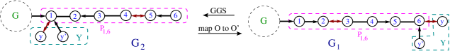
Figure 5. An example of oriented vertices mapped from $B\cap P_{1,k}$ to $B^{\prime}\cap P_{1,k}$.

Enumerating the sets $\mathcal{O}_{G_{2},r}(\mu)$ and $\mathcal{O}_{G_{1},r}(\mu)$ using Lemma 12, we get $|\mathcal{O}_{G_{2},r}(\mu)|\leq|\mathcal{O}_{G_{1},r}(\mu)|$ for all $r\geq 0$ and for all $\mu\in P(n)$. Thus combining Lemmas 6 and 9 with Lemma 12 gives a proof of the following result which gives Theorem 2 as an easy consequence.

Theorem 13.

Let $G_{1}$ and $G_{2}$ be two bipartite graphs with $n$ vertices such that $G_{2}=\mathrm{GGS}(G_{1})$. Then for all $r\geq 0$ and for all $\mu\in P(n)$, we assert that $a_{G_{2},r}(\mu)\leq a_{G_{1},r}(\mu).$ Consequently, we have $b_{\lambda,r}(L_{G_{2}})\leq b_{\lambda,r}(L_{G_{1}})$ for all $\lambda\vdash n$.

Thus, $\mathrm{GGS}$ operation decreases each coefficient of the Laplacian immanantal polynomial of a bipartite graph. Also taking $r=n$ in Theorem 13 concludes that the $\mathrm{GGS}$ operation on a bipartite graph decreases each Laplacian immanant $\mathrm{imm}_{\lambda}(L_{G})$ indexed by $\lambda$. Further using Lemma 4 and Theorem 13, we solve the following extreme value problem of finding the max-min pair in $\Omega_{C_{2k}}^{v}(n)$ for each $b_{\lambda,r}(L_{G})$

Corollary 14.

Going up along $\mathrm{GGS}$ poset of $\Omega_{C_{2k}}^{v}(n)$ decreases each coefficient of the Laplacian immanantal polynomial of a unicyclic graph in absolute value. Consequently, the max-min pair for these coefficients in absolute value is $(G_{P_{n-2k+1}},G_{S_{n-2k+1}})$ in the set $\Omega_{C_{2k}}^{v}(n)$.

6. Generalized matrix function indexed by symmetric functions

For a positive integer $n$, let $\mathsf{SF}_{n,\mathbb{Q}}$ denote the vector space of degree $n$ symmetric functions over $\mathbb{Q}$, the set of rational numbers. Thus, each symmetric function $\tau$ of $\mathsf{SF}_{n,\mathbb{Q}}$ can be written as a linear combination of basis vectors of $\mathsf{SF}_{n,\mathbb{Q}}$. In the theory of algebraic combinatorics which involves symmetric functions, the vector space $\mathsf{SF}_{n,\mathbb{Q}}$ has six standard bases. In this paper, standard terminology is used to denote each of the usual bases of $\mathsf{SF}_{n,\mathbb{Q}}$. Thus for a given $\lambda\vdash n$, the Schur, power sum, elementary, homogeneous, monomial and forgotten symmetric functions are denoted by $s_{\lambda}$, $p_{\lambda}$, $e_{\lambda}$, $h_{\lambda}$, $m_{\lambda}$ and $f_{\lambda}$, respectively. We refer the reader to the textbooks by Stanley [20] and by Mendes and Remmel [11] for background on symmetric functions. It is well known that $\mathsf{SF}_{n,\mathbb{Q}}$ has an inner product structure as well. Another inner product space often studied is $\mathsf{CF}_{n}$, the space of class functions from $\mathfrak{S}_{n}\mapsto\mathbb{C}$. Further, there is a well known isometry between these two spaces called the Frobenius characteristic, denoted $\mathsf{ch}:\mathsf{CF}_{n}\rightarrow\mathsf{SF}_{n,\mathbb{Q}}$ (see [20] for more details).

Let $T$ be a tree on $n$ vertices with Laplacian matrix $L_{T}$. From Sections 1, 3 and 5, we recall that inequalities involving coefficients of the Laplacian immanantal polynomial of $T$ are known as we go up along $\mathrm{GTS}_{n}$ poset. For each $\lambda\vdash n$, it is well known that the inverse Frobenius image $\mathsf{ch}^{-1}_{s_{\lambda}}$ of the Schur symmetric function $s_{\lambda}$ is $\chi_{\lambda}$, the irreducible character of $\mathfrak{S}_{n}$ over $\mathbb{C}$ indexed by $\lambda$. Thus using the Frobenius characteristic map $\mathsf{ch}(\cdot)$, this can be thought as a result associated with the Schur symmetric function $s_{\lambda}$ (see Nagar and Sivasubramanian [16] for more details). In [16] authors introduced a generalized matrix function on the set of square matrices associated with an arbitrary symmetric function. Further they proved that going up $\mathrm{GTS}_{n}$ decreases the absolute value of each coefficient of generalized matrix polynomial associated with $s_{\lambda}$, $p_{\lambda}$, $e_{\lambda}$, $h_{\lambda}$, $m_{\lambda}$ and $f_{\lambda}$ for each partition $\lambda$ of $n$.

For $\tau\in\mathsf{SF}_{n,\mathbb{Q}}$, let $\mathsf{ch}^{-1}_{\tau}=\mathsf{ch}^{-1}(\tau)$ be the inverse Frobenius image of $\tau$. Clearly, $\mathsf{ch}^{-1}_{\tau}\in\mathsf{CF}_{n}$ is a class function on $\mathfrak{S}_{n}$ over $\mathbb{C}$ indexed by $\tau$. From [16] we recall the following definition of the generalized matrix function ($\mathrm{GMF}$ henceforth) of a matrix $A=(a_{i,j})\in{\mathbb{M}}_{n}(\mathbb{C})$ associated with $\tau$. It is denotes as $\mathrm{GMF}_{\tau}(A)$ and it is defined by

(6) $$\mathrm{GMF}_{\tau}(A)=\sum_{\psi\in\mathfrak{S}_{n}}\mathsf{ch}^{-1}_{\tau}(\psi)\prod_{i=1}^{n}a_{i,\psi(i)}.$$

Using (6), when $\tau=s_{\lambda}$ it is simple to see that $\displaystyle\mathrm{GMF}_{\tau}(A)=\mathrm{imm}_{\lambda}(A)$. Inspired by immanantal polynomial, the generalized matrix polynomial of a matrix $A$ associated with $\tau$ denoted as $\phi_{\tau}(A,x)$ is defined by $\phi_{\tau}(A,x)=\mathrm{GMF}_{\tau}(xI-A)$. Thus when $\tau=s_{\lambda}$, we have $\mathrm{GMF}_{\tau}(xI-A)=\mathrm{imm}_{\lambda}(xI-A)$, an immanantal polynomial of $A$ indexed by $\lambda$. In particular, when $\lambda=1^{n}$ and $\tau=s_{\lambda}$, $\mathrm{GMF}_{\tau}(xI-A)$ is the characteristic polynomial of $A$.

Let $G$ be a graph with $n$ vertices and let $L_{G}=(\ell_{i,j})_{1\leq i,j\leq n}$ be its Laplacian matrix. Thus from (6), the generalized matrix function $\mathrm{GMF}_{\tau}(L_{G})$ of $L_{G}$ associated with $\tau\in\mathsf{SF}_{n,\mathbb{Q}}$ is given by

$$\mathrm{GMF}_{\tau}(L_{G})=\sum_{\psi\in\mathfrak{S}_{n}}\mathsf{ch}^{-1}_{\tau}(\psi)\prod_{i=1}^{n}\ell_{i,\psi(i)}.$$

and the generalized matrix polynomial of $L_{G}$ indexed by $\tau$ is given by $\phi_{\tau}(L_{G},x)=\mathrm{GMF}_{\tau}(xI-L_{G})$. It is very easy to show the following counterpart of Lemma 7. Since the proof is a verbatim copy, we omit it.

Theorem 15.

Let $L_{G}$ be the Laplacian matrix of a bipartite graph $G$ with $n$ vertices. Then for all $\tau\in\mathsf{SF}_{n,\mathbb{Q}}$, we assert that $\displaystyle\mathrm{GMF}_{\tau}(L_{G})=\sum\limits_{\mu\in P(n)}\alpha_{\mu}(\tau)a_{G}(\mu)$, where $\displaystyle\alpha_{\mu}(\tau)=\sum\limits_{\nu\in P(n)}\mathsf{ch}^{-1}_{\tau}(\nu)\binom{\mu}{\nu}.$

Since $\chi_{\lambda}=\mathsf{ch}^{-1}_{s_{\lambda}}$, we have $\displaystyle\alpha_{\mu}(\tau)=\alpha_{\lambda,\mu}$ and hence $\displaystyle\mathrm{GMF}_{\tau}(L_{G})=\mathrm{imm}_{\lambda}(L_{G})$. It is very simple to show the following counterpart of Lemma 9. Since the proof is identical, we omit it and merely state the result.

Lemma 16.

Let $G$ be a bipartite graph on $n$ vertices with Laplacian matrix $L_{G}$. Then, for all $\tau\in\mathsf{SF}_{n,\mathbb{Q}}$, we have $\displaystyle\mathrm{GMF}_{\tau}(xI-L_{G})=\sum\limits_{r=0}^{n}(-1)^{r}b_{\tau,r}(L_{G})x^{n-r}$, where $\displaystyle b_{\tau,r}(L_{G})=\sum\limits_{\mu\in P(n)}\alpha_{\mu}(\tau)a_{G,r}(\mu)$ and $r\in\{0,1,\ldots,n\}$.

As mentioned earlier, the inverse Frobenius image $\mathsf{ch}^{-1}_{s_{\lambda}}$ of the Schur symmetric function $s_{\lambda}$ is $\chi_{\lambda}$, the irreducible character of $\mathfrak{S}_{n}$ over $\mathbb{C}$ indexed by $\lambda$. Thus, if any symmetric function $\tau\in\mathsf{SF}_{n,\mathbb{Q}}$ is Schur-positive (that is, $\tau=\sum_{\lambda\vdash n}c_{\lambda}s_{\lambda}$ where $c_{\lambda}\in\mathbb{R}^{+}$ for all $\lambda\vdash n$), then, by linearity, Lemma 6 will be true with $\chi_{\lambda}$ replaced by $\mathsf{ch}^{-1}(\tau)$ in the definition of $\alpha_{\lambda,\mu}$ in (4). Since $h_{\lambda}$ and $e_{\lambda}$ are Schur-positive (see [20, Corollary 7.12.4]), it follows from Theorem 15 that $\alpha_{\mu}(h_{\lambda})\geq 0$ and $\alpha_{\mu}(e_{\lambda})\geq 0$ for all $\lambda,\mu\vdash n$. Since the inverse Frobenius image $\mathsf{ch}^{-1}_{p_{\lambda}}$ of $p_{\lambda}$ is a scalar multiple of the indicator function of the conjugacy class $C_{\lambda}$ indexed by $\lambda$ (see [20]), it follows that $\alpha_{\mu}(p_{\lambda})\geq 0$ for all $\lambda,\mu\vdash n$. We record these well known facts below for future use.

Lemma 17.

For $\lambda,\mu\in P(n)$ and $\tau\in\{e_{\lambda},p_{\lambda},h_{\lambda}\}$, let $\alpha_{\mu}(\tau)$ be as used in Theorem 15. Then $\alpha_{\mu}(\tau)$ is a non-negative integer.

For all $\lambda,\mu\vdash n,$ it is very simple to check that the above lemma is not true when $\tau=m_{\lambda}$, the monomial symmetric function associated with $\lambda$. When $n=4$ the values of the quantity $\alpha_{\mu}(m_{\lambda})$ are tabulated in Table 2. When $\mu=4$ from Table 2, one can see that $\alpha_{\mu}(m_{1^{4}})=-1$, $\alpha_{\mu}(m_{2^{2}})=-2$ and $\alpha_{\mu}(m_{3,1})=-4$. Although when $\mu=2^{j},1^{n-2j}$, Nagar and Sivasubramanian [16] proved that $\alpha_{\mu}(m_{\lambda})$ is a non-negative integral multiple of $2^{j}$ for each $\lambda$ and for all $j\geq 0$.

$$\begin{array}[]{|l | c | c|c |c|c|}\hline\cr&\mu=1^{4}&\mu=2,1^{2}&\mu=2^{2}&\mu=3,1&\mu=4\\ \hline\cr\lambda=1^{4}&1&0&0&0&-1\\ \hline\cr\lambda=2,1^{2}&0&0&0&0&\ \ \ 4\\ \hline\cr\lambda=2^{2}&0&0&0&0&-2\\ \hline\cr\lambda=3,1&0&0&0&0&-4\\ \hline\cr\lambda=4&0&0&0&0&\ \ \ 4\\ \hline\cr\end{array}$$

Table 2. The values of $\alpha_{\mu}(m_{\lambda})$, where $\lambda,\mu\vdash 4.$

Here, we extend Theorem 2 to the generalized matrix polynomials of the Laplacian matrix $L_{G}$ of a bipartite graph $G$ associated with three standard bases involving $e_{\lambda}$, $h_{\lambda}$ and $p_{\lambda}$ for all $\lambda\vdash n$. In other words, we consider the cases when we replace the Laplacian immanantal polynomial $\mathrm{imm}_{\lambda}(xI-L_{G})$ of a bipartite graph $G$ by $\mathrm{GMF}_{\tau}(xI-L_{G})$ in Theorem 2, where $\tau\in\{e_{\lambda},h_{\lambda},p_{\lambda}\}$. Thus using the $\mathrm{GGS}$ operation on a bipartite graph, we have the following consequence of Lemmas 12, 16 and 17 and Theorem 2.

Theorem 18.

For $0\leq r\leq n$ and for all $\lambda\vdash n$, the $\mathrm{GGS}$ operation on a bipartite graph $G$ decreases the coefficient $b_{\tau,r}(L_{G})$ of $(-1)^{r}x^{n-r}$ in $\mathrm{GMF}_{\tau}(xI-L_{G})$, where $\tau\in\{s_{\lambda},e_{\lambda},p_{\lambda},h_{\lambda}\}$. Moreover for this monotonicity result on $\mathrm{GGS}$ poset of $\Omega_{C_{2k}}^{v}(n)$, the max-min pair of unicyclic graphs in $\Omega_{C_{2k}}^{v}(n)$ is $(G_{P_{n-2k+1}},G_{S_{n-2k+1}})$.

Thus the above result solves an extreme value problem involving coefficients of the generalized matrix polynomial of the Laplacian of a bipartite graph associated with the Schur, elementary, power sum and homogeneous symmetric functions.

7. Corollaries

For the convenience of the reader, from [5, 6], we repeat some proofs which go through for an arbitrary graph under $\mathrm{GGS}$ operation thus making our exposition self contained. The important point to note here is a natural extension of monotonicity results on $\mathrm{GTS}_{n}$ to all connected graphs under $\mathrm{GGS}$ operation and it is used to solve extreme value problems of finding the max-min pair in the set $\Omega_{C_{k}}^{v}(n)$ for some graph-theoretical parameters which are monotonic under this transformation. Let $G$ be a graph with adjacency matrix $A(G)$ and spectral radius $\sigma(G)$ (the largest eigenvalue of $A(G)$). Since the proof of the following theorem is identical to the result given in [6, Theorem 3.1], we give an outline of the proof.

Theorem 19.

The $\mathrm{GGS}$ operation on an arbitrary graph increases the spectral radius.

Proof.

Let $G_{1}$ and $G_{2}$ be two arbitrary graphs with $n$ vertices such that $G_{2}=\mathrm{GGS}(G_{1})$. Let $1$ and $k$ be the recipient and the donor in $G_{1}$, respectively. Let $\sigma(G_{1})$ and $\sigma(G_{2})$ be spectral radii of $G_{1}$ and $G_{2}$, respectively. Let $w=(w_{1},w_{2},\ldots,w_{n})^{t}$ be the Perron eigenvector of $A(G_{1})$ associated to $\sigma(G_{1})$ with $||w||=1$. Recall that if the role of $1$ and $k$ in $G_{1}$ are exchanged then the resulting graph after using $\mathrm{GGS}$ transformation is isomorphic to $G_{2}$. Thus without loss of generality, we assume that $w_{1}\geq w_{k}.$ Let $Z_{G_{1}}(k)=\{v\in G_{1}:v\in N(k)\mbox{ with }v\neq k-1\}$, where $N(k)$ is the set of neighbours of $k$ which doesn’t contain $k$. Then it is easy to check that

$$\sigma(G_{1}) =w^{t}A(G_{1})w=w^{t}A(G_{2})w-2(w_{1}-w_{k})\sum_{j\in Z_{G_{1}}(k)}w_{j}$$

$$\leq w^{t}A(G_{2})w\leq\max_{||z||=1}z^{t}A(G_{2})z=\sigma(G_{2}).$$

Hence $\sigma(G_{1})\leq\sigma(G_{2})$ completes the proof. ∎

The main point to note about the above theorem is that it is also true when $G_{2}=\mathrm{GGS}(G_{1})$ and all edges of $G_{1}$ as well as of $G_{2}$ are replaced by blocks (complete graphs).

Let $G$ be a connected graph with $n$ vertices. The Wiener Index of $G$, denoted $\mathrm{Wi\_Index}(G)$ is defined by $\mathrm{Wi\_Index}(G)=\sum_{i,j\in G}d_{G}(i,j)$, where $d_{G}(i,j)$ is the shortest distance between the vertices $i$ and $j$ in $G$. Since the proof of the following theorem is similar to the proof given in [5, Theorem 3.1] we sketch our proof for the sake of completeness.

Theorem 20.

Let $G_{1}$ and $G_{2}$ be two connected graphs with $n$ vertices such that $G_{2}=\mathrm{GGS}(G_{1})$. Then $\mathrm{Wi\_Index}(G_{1})\geq\mathrm{Wi\_Index}(G_{2})$.

Proof.

Let $d_{G_{1}}(i,j)$ be the shortest distance between $i$ and $j$ in $G_{1}$ and similarly $d_{G_{2}}(u,v)$ is defined for $u,v\in G_{2}$. Let $X$ and $Y$ be two subgraphs of $G_{1}$ as given in Figure 2. Thus using Figure 2, it is easy to see that

$$d_{G_{1}}(i,x)+d_{G_{1}}(k+1-i,x)=d_{G_{2}}(i,x)+d_{G_{2}}(k+1-i,x)\mbox{ for all }x\in X$$

and

$$d_{G_{1}}(i,y)+d_{G_{1}}(k+1-i,y)=d_{G_{2}}(i,y)+d_{G_{2}}(k+1-i,y)\mbox{ for all }y\in Y.$$

Obviously $d_{G_{1}}(x_{1},x_{2})=d_{G_{2}}(x_{1},x_{2})$ for all $x_{1},x_{2}\in X$ and $d_{G_{1}}(y_{1},y_{2})=d_{G_{2}}(y_{1},y_{2})$ for all $y_{1},y_{2}\in Y$. It is also easy to check that $d_{G_{1}}(x,y)=d_{G_{2}}(x,y)+(k-1)\mbox{ for all }x\in X\mbox{ and }y\in Y$ and hence

$$\sum_{x\in X,y\in Y}d_{G_{1}}(x,y)=\sum_{x\in X,y\in Y}d_{G_{2}}(x,y)+(k-1)|X||Y|.$$

After combining all the above identities, we assert that $\sum_{i,j\in G_{1}}d_{G_{1}}(i,j)\geq\sum_{u,v\in G_{2}}d_{G_{2}}(u,v)$. Thus $\mathrm{Wi\_Index}(G_{1})\geq\mathrm{Wi\_Index}(G_{2})$ completes the proof. ∎

Thus each monotonic result under $\mathrm{GGS}$ operation is a natural extension of $\mathrm{GTS}$ transformation. Using the definition of $\mathrm{GGS}$ poset on the set $\Omega_{C_{k}}^{v}(n)$, the following result is an easy consequence of Lemma 4 and Theorems 19 and 20.

Corollary 21.

Let $G_{S}=G_{S_{n-k+1}}$ and $G_{P}=G_{P_{n-k+1}}$ be the maximal and the minimal elements in $\Omega_{C_{k}}^{v}(n)$, respectively. Then from Theorems 19 and 20 with Lemma 4, $(G_{S},G_{P})\in\Omega_{C_{k}}^{v}(n)$ is the max-min pair for the spectral radius while $(G_{P},G_{S})\in\Omega_{C_{k}}^{v}(n)$ is the max-min pair for the Wiener index.

In the above corollary if $C_{k}$ is replaced by an arbitrary connected graph $H$ with $k$ vertices, then using Remark 5 we have a $\mathrm{GGS}_{n}$ poset on the set $\Omega_{H}^{v}(n)$ of unlabeled connected graphs with $n$ vertices. This poset also has monotonicity properties for the graph-theoretic parameters given in Corollary 21. Hence for these parameters, the max-min pairs can be determined in the set $\Omega_{H}^{v}(n)$.

Associated to a tree are different notion of Randic index, Geometric index and Atom Bond Connectivity (ABC) index. It would be nice to see the behavior of these graph-theoretic indices under the $\mathrm{GGS}$ operation.

References

- [1] Brown, J., Colbourn, C., and Devitt, J. Network Transformations and Bounding Network Reliability. Networks 23 (1993), 1–17.
- [2] Chan, O., and Lam, T. K. Binomial Coefficients and Characters of the Symmetric Group. Technical Report 693 (1996), National Univ of Singapore.
- [3] Chan, O., and Lam, T. K. Vertex Orientations and Immanants of Bipartite Graphs. Available on Semantic Scholar https://www.semanticscholar.org/paper/Vertex-Orientations-and-Immanants-of-Bipartite-LamAugust/22b4a499602478538cd048bc7ae2a57e9303dff0 (1997).
- [4] Chan, O., and Lam, T. K. Hook Immanantal Inequalities for Trees Explained. Linear Algebra and its Applications 273 (1998), 119–131.
- [5] Csikvári, P. On a Poset of Trees. Combinatorica 30 (2) (2010), 125–137.
- [6] Csikvári, P. On a Poset of Trees II. Journal of Graph Theory 74 (2013), 81–103.
- [7] Gutman, I., and pavlović, L. On the Coefficients of the Laplacian Characteristic Polynomial of Trees. Bulletin Académie Serbe des sciences et des art 28 (2003), 31–40.
- [8] Gutman, I., and Zhou, B. A connection between ordinary and Laplacian spectra of bipartite graphs. Linear and Multilinear Algebra 56 (3) (2008), 305–310.
- [9] Kelmans, A. K. On Graphs with Randomly Deleted Edges. Acta Mathematica Acad. Sci. Hungarica 37 (1981), 77–88.
- [10] Lieb, E. H. Proof of some Conjectures on Permanents. Journal of Math and Mech 16 (1966), 127–134.
- [11] Mendes, A., and Remmel, J. B. Counting with Symmetric Functions. Developments in mathematics. Springer, Cham, 2015.
- [12] Mohar, B. On the Laplacian coefficients of acyclic graphs. Linear Algebra and its Applications 722 (2007), 736–741.
- [13] Nagar, M. K. Eigenvalue monotonicity of q-laplacians of trees along a poset. Linear Algebra and its Applications 571 (2019), 110–131.
- [14] Nagar, M. K., and Sivasubramanian, S. Hook immanantal and Hadamard inequalities for -Laplacians of trees. Linear Algebra and its Applications 523 (2017), 131–151.
- [15] Nagar, M. K., and Sivasubramanian, S. Laplacian immanantal polynomials and the GTS poset on trees. Linear Algebra and its Applications 561 (2019), 1–23.
- [16] Nagar, M. K., and Sivasubramanian, S. Generalized Matrix polynomials of Tree Laplacians indexed by Symmetric functions and the GTS poset. Séminaire Lotharingien de Combinatoire B83a (2021), 10pp.
- [17] Sagan, B. E. The Symmetric Group: Representations, Combinatorial Algorithms, and Symmetric Functions, 2nd ed. Springer Verlag, 2001.
- [18] Satyanarayana, A., Schoppman, L., and Suffel, C. L. A Reliability-Improving Graph Transformation with Applications to Network eliability. Networks 22 (1992), 209–216.
- [19] Schur, I. Über endliche Gruppen und Hermitesche Formen. Math. Z. 1 (1918), 184–207.
- [20] Stanley, R. P. Enumerative Combinatorics, vol 2. Cambridge University Press, 2001.