Fingerprints of Generative Models in the Frequency Domain

Abstract

It is verified in existing works that CNN-based generative models leave unique fingerprints on generated images. There is a lack of analysis about how they are formed in generative models. Interpreting network components in the frequency domain, we derive sources for frequency distribution and grid-like pattern discrepancies exhibited on the spectrum. These insights are leveraged to develop low-cost synthetic models, which generate images emulating the frequency patterns observed in real generative models. The resulting fingerprint extractor pre-trained on synthetic data shows superior transferability in verifying, identifying, and analyzing the relationship of real CNN-based generative models such as GAN, VAE, Flow, and diffusion.

1 Introduction

In recent years, advanced generative modeling technologies have revolutionized various fields such as art creation, design, and human-computer interaction [1; 2; 3; 4]. Despite their positive and beneficial applications, new concerns have arisen. On the one hand, copyrighted generative models can be copied and distributed, leading to potential copyright infringement issues. On the other hand, they can be utilized to generate illegal and malicious content, posing significant challenges to content moderation and social harm prevention. To address these issues, model attribution,  i.e., the process of identifying the source model of generated content, has recently garnered increasing attention [5; 6; 7; 8; 9; 10].

Several studies [5; 6] confirmed that generative models could leave unique fingerprints on their output images. Further works demonstrated the feasibility of attributing generated images to a limited set of models [11; 7; 8; 9]. Considering an unlimited number of unknown models in the open-world scenarios, recent works  [10; 12] began to consider solving model attribution in an open-set formalization. However, the problem of model attribution remains unsolved. Existing solutions are limited by the known/unknown unbalance issue in real-world scenarios, where only a limited number of known models could be sampled while the number of unknown models continues to grow. Furthermore, there was little effort put into investigating the cause of fingerprints of generative models, namely, how the fingerprints depend on the network’s architecture and specific parameters. Understanding this is an important first step toward more effective model attribution algorithms.

Our interest in analyzing the problem is triggered by the observation that different generative models exhibit frequency pattern discrepancies on spectra. See Fig. 1, the major differences lie in two aspects: 1) frequency distribution, where the magnitudes of high and low-frequency components differ across the spectra. 2) grid-like patterns with varying strengths and periodicity. Then we tend to give explanations for these frequential discrepancies by interpreting network components in the frequency domain. We discover that the element-wise multiplication of spectra with the convolution kernel leads to a uniform frequency distribution pattern in the high-frequency components. Grid-like patterns are derived by upsampling-induced spectrum replication, which are further modified by upsampling kernels. Throughout the generation process, frequency patterns from preceding blocks would be repeated by upsampling layers, accumulated layer by layer in a multiplication form with spectra of convolution filters, weakened or enhanced by activation and normalization layers, eventually forming the frequency pattern on output images.

Leveraging the insights gained from our analysis, we seek to alleviate the known/unknown-unbalanced model attribution problem by constructing a variety of synthetic models that exhibit frequency patterns similar to genuine generative models, but at a much lower cost. Specifically, we leverage small generative blocks with varied architectures and parameters to simulate diverse frequency patterns. Based on our analysis of frequency pattern attenuation over generative blocks, these blocks could simulate prominent frequency patterns for many common generative models. We also synthesize diverse upsampling grids by noise-to-noise generators involving multiple deconvolution-based upsampling blocks.

The fingerprint extractor pre-trained on the synthetic data in a metric learning framework shows superior transferability on various types of real CNN-based generative models, such as GAN, VAE, Flow, diffusion, and state-of-the-art Text2Image models. We explore its application in various attribution scenarios, including model verification, open-set model identification, and model lineage analysis. Experimental results show that the fingerprint extractor achieves over 95% model verification accuracy on real generative models with only 10 samples, and superior open-set model identification performance with much fewer samples involved in training. The fingerprint extractor also exhibits the potential to link different versions of models with finetuning relationships. Our key contributions are as follows:
$\bullet$ We make the first attempt to investigate the formation of model fingerprints of CNN-based generative models in the frequency domain.
$\bullet$ We pioneer solving the known-unknown-unbalanced model attribution problem by pre-training on large-scale low-cost synthetic data in a metric-learning framework.
$\bullet$ Extensive evaluations demonstrate the superior transferability of the pre-trained fingerprint extractor in verifying, identifying, and analyzing the relationship of real CNN-based generative models.

StarGAN

SNGAN

VanillaVAE

Glow

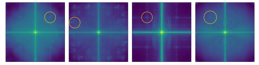
Figure 1: Averaged spectra of high-passed samples generated by different generative models trained on CelebA [13] dataset (low frequencies are shifted to the center on the spectra). As seen, the frequency discrepancy between different models mainly exists in frequency distribution and grid-like patterns (yellow circles).

2 Related work

Frequency bias of generative models. Existing studies [14; 15; 16; 17; 18] have identified frequency discrepancies between generated and real images and attempted to provide explanations. Some of these studies [14; 15; 16] attribute this phenomenon to upsampling operations, which generate an excess of high frequencies in the spectral statistics. Other studies [17; 18] attribute it to linear dependencies in the spectrum of convolutional filters, which impede the learning of high frequencies. However, most studies have only analyzed the differences between real and fake images, with fewer studies examining the differences between images generated by different models.

Generative model attribution. Generative image attribution aims to identify the corresponding generative model based on the generated image and can be divided into active attribution [19; 20; 21] and passive attribution [5; 6; 8]. Active attribution involves injecting fingerprints into generative models through weight modulation or training on fingerprinted datasets, but there is no analysis of how fingerprint information is embedded into generative models. Passive attribution tries to extract the intrinsic fingerprints of generative models. Recent work by Marra  et al. [5] uses averaged noise residuals to represent model fingerprints and finds that model fingerprints are periodic. Later works  [6; 8; 9] further verify the existence of model fingerprints and achieve high accuracy on a fixed and finite set of models following a closed-set classification formulation. Yang  et al. [10] first considers the open-set model attribution problem, but can still only recognize new models as unknown without identifying them. In our work, we provide empirical explanations for the cause of intrinsic model fingerprints in the frequency domain and move towards attributing unseen models in the open world.

3 Frequential fingerprints of generative models

Model fingerprints, which serve as unique characteristics in generated images that differentiate different models, despite having been found to exist, have received little understanding regarding where they exist. The primary reason is they are visually imperceptible in the spatial domain. We begin to analyze them by observing the spectra of images generated by various generative models. See Fig. 1, two distinct features could be observed on the spectra: 1) Grid-like patterns exhibiting varying strengths and periodicity (highlighted by yellow circles). 2) Frequency distribution across the entire spectrum, where the magnitudes of high and low-frequency components differ among the spectra. However, the underlying causes of these frequency patterns have received little attention thus far. In the following sections, we aim to provide empirical explanations for the formation of these patterns through an analysis of the generation process in the frequency domain.

3.1 Network components analysis in the frequency domain

Different generative models exhibit variations in terms of training objectives, regularizations, and architectures, making it a daunting task to consider all these factors. In this work, we specifically focus on the “decoder", which reconstructs or generates the output image from latent representations and directly influences the output images. The latent representations could be obtained from a preceding encoder or directly sampled from a pre-defined distribution. The structure of a typical decoder is analogous among many generative models such as Generative Adversarial Networks (GAN), Variational Autoencoders (VAE), and Diffusion models. Typically, a decoder is composed of multiple blocks, with each block upscaling and refining input feature maps through the incorporation of upsampling, convolution, normalization, and activation layers. In this section, we delineate how each of these components operates in the frequency domain and how they contribute to the creation or transformation of frequency patterns. Note that the DFT frequency spectrums in this section are not shifted to better observe the high-frequency regions. Thus, the corner regions correspond to low frequencies, while the center regions correspond to high frequencies.

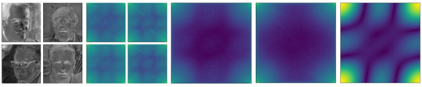
(a) Feature maps $256^{2}$

(b) DFT spectrums

(c) Mean map

(d) Variance map

(e) Convolution spectrum

Figure 2: (a) Four feature maps output by the same convolutional layer of a StyleGAN2 face generator with different latent codes. (b) DFT magnitude spectrums of the feature maps. (c)(d) Mean and variance map of feature spectrums over 1000 latent codes. (e) Averaged spectrum of 64 kernels in the convolution layer that generates the feature map.

Frequency distribution pattern caused by convolution. For an input feature map $X\in\mathbb{R}^{C_{1}\times H\times W}$ and a convolution layer with kernels $K\in\mathbb{R}^{C_{1}\times C_{2}\times k\times k}$ with stride one, where $C_{1}$, $C_{2}$, and $k$ are input channel number, output channel number, and kernel size, respectively. We first consider a simple case with single input and output channel,  i.e., $C_{1}=1$ and $C_{2}=1$. According to the Convolution Theorem [22], the spatial convolution operation equals to multiplication operation in the frequency domain:

$$\mathcal{F}\{X\otimes K\}=\mathcal{F}\{X\}\cdot\mathcal{F}\{K\},$$ (1)

where $\mathcal{F}\{X\}$ and $\mathcal{F}\{K\}$ are the discrete Fourier transform (DFT) of zero-padded $X$ and $K$. In the case of multiple channels, the Convolution Theorem still stands for the convolution computation of each channel:

$$\mathcal{F}\{O_{j}\}=\mathcal{F}\{\sum_{i=0}^{C_{1}}X_{i}\otimes K_{i,j}\}=\sum_{i=0}^{C_{1}}\mathcal{F}\{X_{i}\}\cdot\mathcal{F}\{K_{i,j}\},$$ (2)

where $O_{j}$ is the $j$-th channel of the output feature map, $X_{i}$ is the $i$-th channel of the input feature map, $K_{i,j}$ is the $(i,j)$-th channel of $K$.

Next, we explain how convolution operations create frequency patterns. Considering the simple case of a single convolution layer operating on 2D Gaussian noises. The spectrum of Gaussian noise still displays like Gaussian noise. Thus, uniform frequency patterns would exist in the spectrum of all output noises that are convolved by this layer and exhibit the shape of the zero-padded convolution kernel’s spectrum according to Eq. 1. This indicates that when different latent codes are sampled into the generator (or decoder), convolutions would produce similar frequency distribution patterns.

Fig. 2 further shows the case of a convolution layer with multiple channels operating on features from the last block of a well-trained StyleGAN2 [23] face generator. See Fig. 2b and  2e, varying the latent code sent into the generator, the spectrums of feature maps output by the same convolutional layer show uniform frequency patterns and are consistently similar to the averaged kernel spectrum of the convolution layer generating them. We also plot the mean and variance map of feature spectrums varying the latent code in Fig. 2c and  2d. The mean map is similar to the convolution spectrum as expected. The variance map exhibit low in the high-frequency region and high in the low-frequency region. This indicates that the variation of latent code would more significantly alter low-frequency components while keeping high-frequency patterns consistent. Thus, generated images from the same generator would share similar high-frequency patterns despite their differences in low-frequency semantics. We also emphasize that this uniform frequency pattern in high-frequencies is observed in common generators that generate low-frequency semantics. However, for other specific generators such as texture generation models, this pattern may manifest in different frequency components.

Grid-like pattern caused by upsampling layer. Common types of upsampling layers are deconvolution (or transposed convolution) and interpolation upsamplers such as nearest neighbor (NN) and bilinear. Deconvolution is equivalent to interleaving the input features with 0’s and applying a standard convolutional operation. For interpolation upsamplers, the interpolated pixels are linearly dependent on their neighbors, thus they could also be regarded as a combined operation including zero-interleaving and a convolution operation with fixed parameters. Then we could summarize upsampling operations into a unified formalization:

$$X_{up}=\text{ZeroInter}(X)\otimes K_{up},$$ (3)

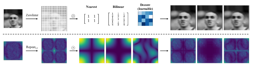
(a)

(b)

(c)

(d)

Figure 3: Upsampling in the spatial (above) and frequency (below) domain. (a) Input sample output by a convolution layer. (b) Zero-interleaved sample. The spectrum exhibits grids in 1/2 position due to replication. (c) Upsampling kernels of nearest neighbor, bilinear, and deconvolution. NN and bilinear kernels naturally suppress high-frequency components in center regions. (d) Output samples by three upsampling layers. Deconvolution produces stronger grids than NN and bilinear.

where ZeroInter is interleaving the input feature $X$ with 0’s, and $K_{up}$ is a convolution kernel. For deconvolution, $K_{up}$ is learnable. For nearest neighbor and bilinear upsampling, $K_{up}$ has a corresponding fixed weight, see Fig. 3c. Adopting the DFT transform, it’s easy to obtain that zero-interleaving in the spatial domain brings about spectrum replicas in the frequency domain. Then we could summarize upsampling operation in the frequency domain as replicating the frequency spectrum of the input signal and pointwise multiplication with a corresponding upsampling kernel’s spectrum:

$$\mathcal{F}\{X_{up}\}=\text{Repeat}_{2,2}(\mathcal{F}\{X\})\odot\mathcal{F}\{K_{up}\},$$ (4)

where $\text{Repeat}_{2,2}$ means repeat the spectrum of $X$ along two frequency dimensions by two times.

Through the formulation, we could attribute the grid-like pattern observed on the spectrum to the zero-interleaving operation in the spatial domain. See Fig. 3b, this operation causes low-frequency components (corners) to shift towards high-frequency regions (center) after spectrum replication, resulting in distinct lines along the horizontal and vertical axes. It can be easily deduced that the periodicity of these grids depends on the number of upsampling layers. $n$ layers of upsampling would result in grids in multiples of $1/2^{n}$ positions. These grids could be polished by following upsampling kernel. See Fig. 3d, NN and bilinear tend to suppress these grids as their spectrums are naturally low in the central regions. On the other hand, deconvolution kernels, which are learned without specific constraints, may not sufficiently suppress these grids like NN and bilinear, leading to stronger grid patterns on the spectrum. This analysis could also provide a unified explanation for the commonly discussed empirical observation that nearest and bilinear produce fewer artifacts than deconvolution [24; 25; 14; 16].

Frequency pattern transformation by normalization and nonlinearity. Common types of normalization are Instance Normalization (IN) and Batch Normalization (BN), which have the same computational form, except that the mean and variance are derived from an instance or a batch. As described in  [26], the implementation of BN in the frequency domain has exactly the same form as the time domain. Thus, the normalization layer would normalize, shift and scale the frequency pattern of the input signal. To give an intuitive understanding of the effect of nonlinear activation functions, an approach is to apply Taylor series approximation to transform them as polynomials, and perform DFT transform based on the convolution theorem that multiplication in the spatial domain is equivalent to convolution in the frequency domain. For example, SReLU [27] uses polynomial fitting to approximate the ReLU function $max(0,x)$ in the form of $0.3x+0.021x^{2}$, which can be calculated in the frequency domain as $0.3X+0.021\cdot(X\otimes X)$, where $X$ is the DFT spectrum of $x$. As seen, the magnitude of the input signal’s frequency pattern would be altered by self-convolution items, and the magnitude of changes depends on the amplitude of the input signal’s spectrum.

3.2 Frequency pattern attenuation over generative blocks

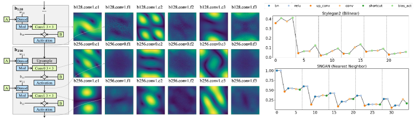
(a)

(b)

(c)

(d)

(e)

(f)

(g)

(h)

Figure 4: Frequency pattern attenuation over generative blocks. (a) The last two blocks of a StyleGAN2 generator. (b,d,f) Averaged convolution kernel spectrum along input channels of three output channels (column marginal) for three convolutional layers b128.conv1, b256.conv0, b256.conv1 (row marginal). (c,e,g) Spectrum of features averaged on 50 samples output by channels on the left. (h) High-frequency component variation throughout the generation process. Different generative blocks are separated by dashed lines.

See Fig. 3c, interpolation upsamplers such as nearest neighbor and bilinear would cause high-frequency attenuation due to their low-pass upsampling filters. Generators like StyleGAN3 [28] even design low-pass filters with larger attenuation to suppress aliasing. These indicate that high-frequency patterns from preceding generative blocks may be filtered out when passed to consequent blocks.

Fig. 4 gives an intuitive illustration of the attenuation. Fig. 4a shows the last two blocks $\mathbf{b_{128}}$ and $\mathbf{b_{256}}$ of a StyleGAN2 [23] $256\times 256$ face generator. Each block increases the resolution by two and contains a Biliner Up+Conv0 layer and a Conv1 layer. We visualize the spectrum (averaged along the input channels) for three output channels (column marginal) in three convolutional layers (row marginal) in Fig. 4(b,d,f), and the spectrum of output features by these output channels in Fig. 4(c,e,g). We could notice the output features’ spectrum of b128.conv1 shares similar patterns with the spectrum of convolution channels on their left. However, after the Upsample and Conv0 layer, the patterns are largely attenuated and show again as the shape of Conv1’s spectrum after another convolution layer. This phenomenon validates that bilinear upsampling layers would cause high-frequency attenuation and thus suppress frequency patterns produced by previous layers.

Fig. 4h further qualifies the high-frequency component variation throughout the generation process. X-axis means every network component in the sequence of generation, and y-axis means the proportion of high frequencies of feature maps output by each network component, which is calculated as the ratio of the sum of values in the latter half of the azimuthal integral spectrum [15] to the sum of all values. As seen, The “up_conv" upsampling layer stably suppresses high-frequency components in every generative block. The high-frequency attenuation phenomenon indicates that the last generative block would play a prominent role in producing model fingerprints for common generators with low-pass upsampling kernels.

4 Pretrained fingerprint extractor based on synthetic data

The above analysis provides insight into the generation process of two key components of model fingerprints: 1) Convolutional operations create uniform frequency patterns in the high-frequency region, which are repeated during upsampling, normalized and altered by normalization and nonlinear activation functions. 2) Upsampling layers cause frequency replication due to zero-interleaving in the spatial domain, resulting in grids in the multiplies of $1/2^{n}$ positions. These grids are most prominent in deconvolution-based generators. Leveraging these observations, we seek to alleviate the known/unknown unbalance problem in model attribution by constructing a large number of synthetic models that exhibit similar frequency patterns to real generative models. By training the fingerprint extractor on simulated data, we can achieve superior transferability to real generative models.

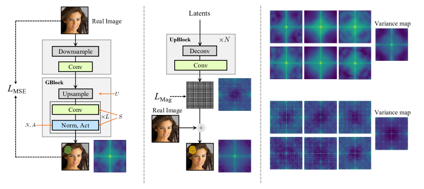
(a)

(b)

(c)

Figure 5: (a) Frequency distribution pattern simulation. (b) Grid pattern simulation. (c) Averaged spectrums of images generated by different frequency distribution pattern generators (above) and noise samples by grid pattern generators (below). Low frequencies are shifted to the center.

Frequency distribution pattern simulation. CNN-based generative models have become increasingly complex with numerous parameters. Simulating the exact frequency patterns left by each individual layer becomes a daunting task. Motivated by the frequency pattern attenuation phenomenon described in Sec. 3.2, we propose to leverage generative blocks to simulate the essential characteristics in generated images, which allows us to strike a balance between computational efficiency and simulating the key frequency patterns. Fig. 5a shows the generative block. The input image is first downscaled by half using a pooling layer. Then, a convolutional layer is applied to increase the feature dimension. The output feature is then sent into a generative block commonly used in real generative models, whose architecture is determined by $\{L,S,U,A,N\}$. $L$ represents the number of convolutional layers in the block. $S$ refers to the order of activation and normalization relative to the convolution layer. $U$ is the upsampling operation that can be nearest neighbor upsampling, bilinear upsampling, or a stride 2 deconvolution layer. $A$ is the activation function that can be ReLU, Sigmoid, Tanh, or no activation. $N$ is the normalization type that can be batch normalization, instance normalization, or no normalization. We train 20 models with different training seeds using reconstruction loss and constrain the minimum reconstruction residual to 0.005, resulting in a total of 20x2x2x3x4x3=2880 models. Due to the simplicity of the reconstruction task, each model’s training only takes seconds to minutes. We admit that the single-generative-block architecture may not perfectly replicate the fingerprints’ complexity of real generative models, especially those that exhibit less high-frequency attenuation utilizing deconvolution as an upsampling layer. While it is rare for two models to have identical parameters in the last generative block, our solution enables the rough simulation of fingerprints.

Grid pattern simulation. We use generators involving multiple deconvolution layers to simulate upsampling grids. See Fig. 5b, the generator contains several upsampling blocks, each composed of a deconvolution layer followed by a convolution layer. We employ a magnitude loss that minimizes the magnitude of the output noise to 0.005. These noise samples are then overlapped with real images, resulting in simulated images with upsampling grids. To ensure the diversity of simulated grids, we train 500 models for each architecture of the grid generators, with the block number varying from 3, 4, to 5. We neither directly use upsampled real images nor the output noise alone, as the former would produce very blur images and the latter would generate that are totally dissimilar to natural images and harms the transferability. Additionally, we refrain from using nearest or bilinear upsampling layers, as they are equipped with fixed upsampling kernels and are unable to produce highly diverse grids. We don’t overlap the output noise from the grid generators with images output by frequency pattern generators, as this would introduce “shortcuts" and prohibit the fingerprint extractor from differentiating each type of pattern.

Type	Dataset	Architecture
GAN	CelebA	ProGAN [29], MMDGAN [30],SNGAN [31], InfoMaxGAN[32], StarGAN [33], AttGAN [34]
	Face-HQ	StyleGAN2 [23], StyleGAN3-t[28], StyleGAN [35], ProGAN, StyleGAN3-r
	Lsun-Bedroom	ProGAN, SNGAN, MMDGAN, InfoMaxGAN
	ImageNet	BigGAN [36], SAGAN [31], S3GAN [37], ContraGAN [38], SNGAN
VAE	CelebA	VanillaVAE [39], BetaVAE [40], DisentangledBetaVAE [41], InfoVAE [42]
Flow	CelebA	Glow [43], ResFlow [44]
Diffusion	Lsun-Bedroom	ADM [45], DDPM [46], LDM [3], PDNM [47]
Text2Image	COCO & user prompts	StableDiffision [3], Midjourney [4], Glide [1], DalleE-2 [2], DalleE-mini [48]

Table 1: Dataset of real generative models including GAN, VAE, Flow, Diffusion, and Text2Image models. Models underlined are known models for the open-set 1vN model identification experiment.

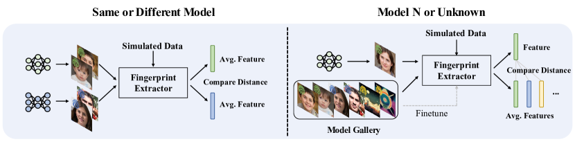
(a) Model verification

(b) Open-set model identification

Figure 6: Two scenarios for model attribution.

Spectrum visualization. In Fig. 5c, we show the averaged spectra of samples generated by different frequency distribution pattern generators and grid pattern generators. The spectra variance map in the last column demonstrates the differences between the two types of generators. The grid pattern generators exhibit diversity primarily within the grid regions, while the frequency distribution pattern generators show diversity throughout the entire spectrum.

Training the fingerprint extractor. We build the synthetic data based on CelebA dataset [13]. For each real image in the dataset, the image is firstly randomly cropped to a size of $128\times 128$ and fed into a randomly selected model from the synthetic model pool. The generated image is then transformed using DFT and the magnitude spectrum is sent to train the fingerprint extractor. We use ResNet50 as the backbone of the fingerprint extractor. The backbone is followed by a classification head and a projection head. The classification head employs a multi-class cross-entropy loss, which guides the classifier to identify the corresponding generator for the input image. The projection head is followed by a triplet loss, which encourages generated images from the same generator to be as similar as possible in the feature space while promoting a larger dissimilarity between images from different generators.

5 Experiments

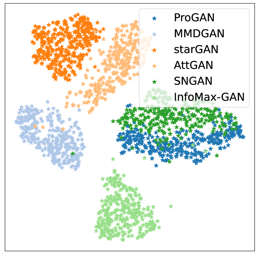
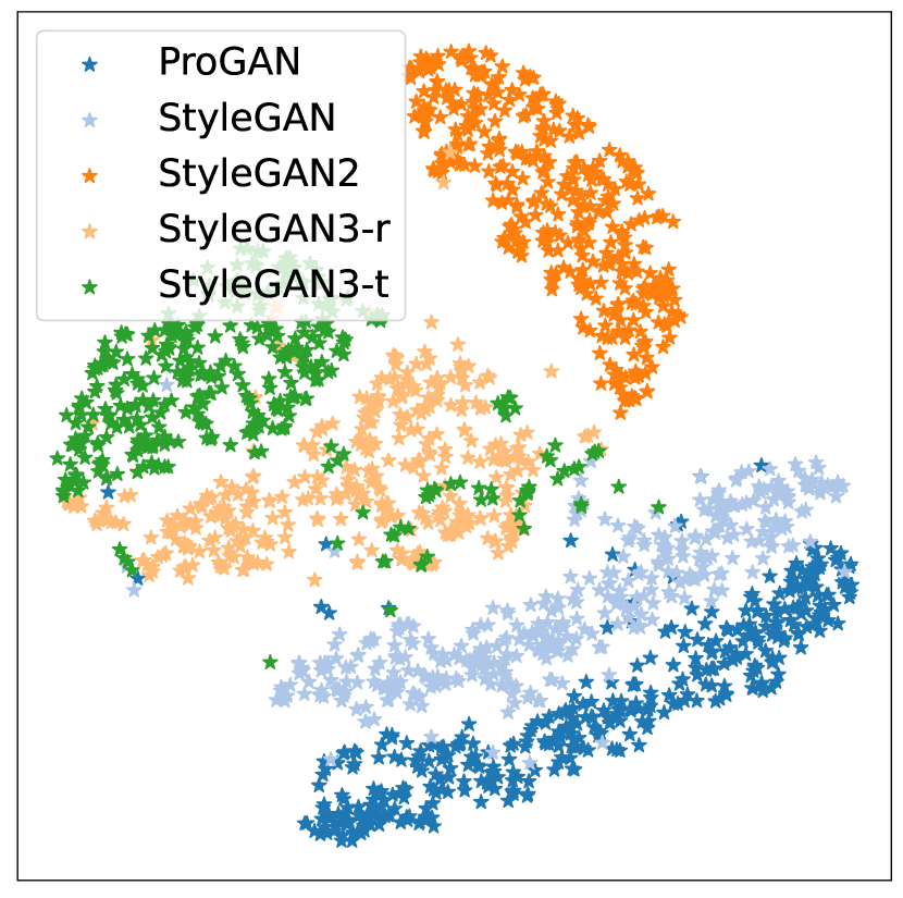
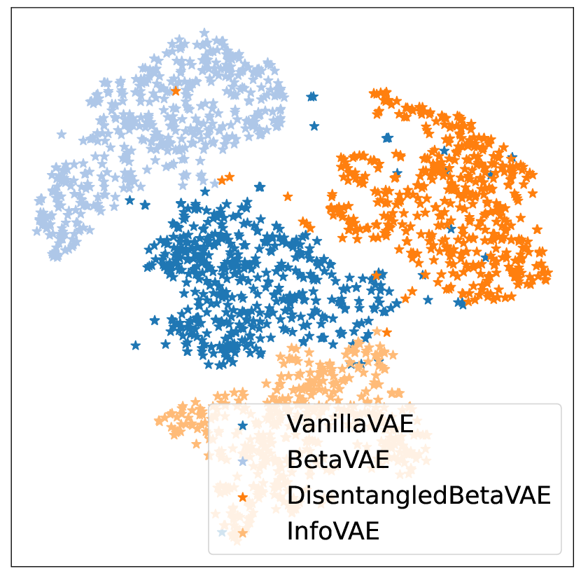
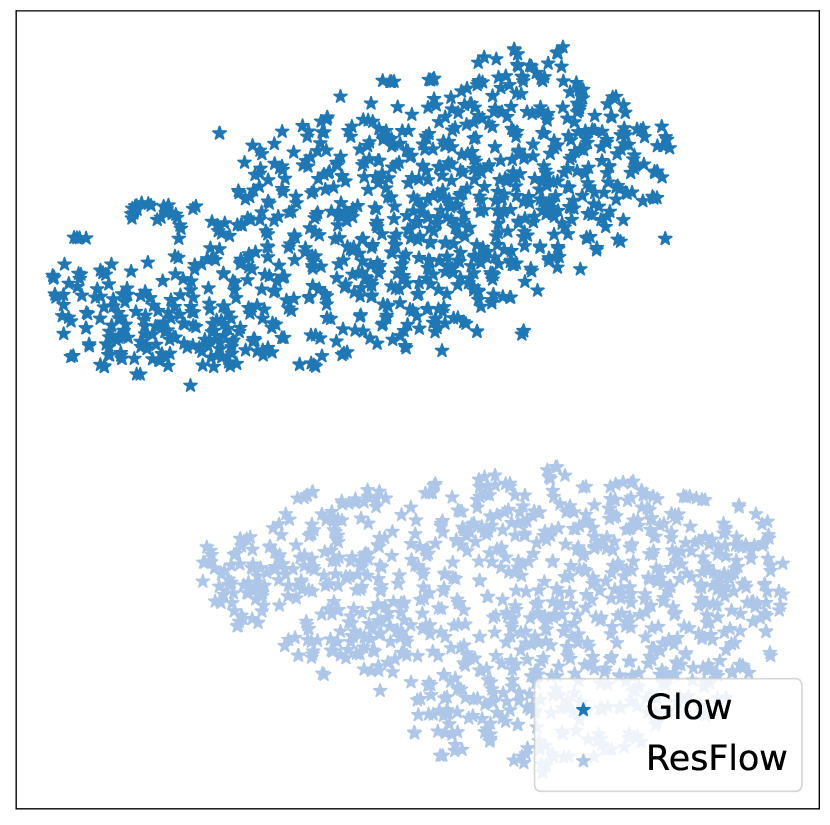
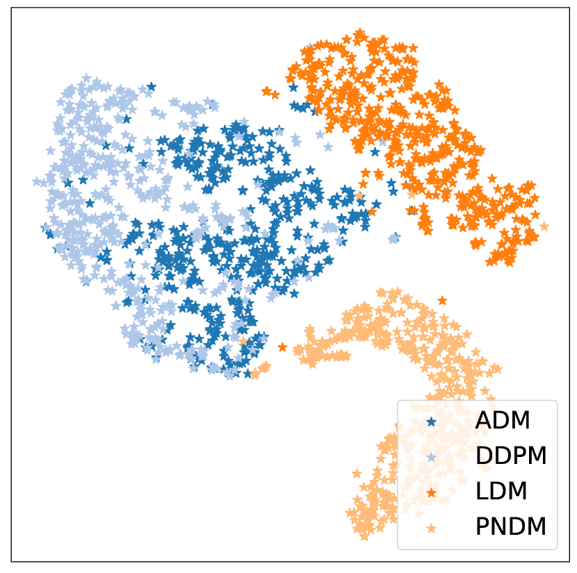
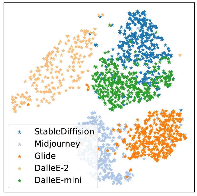
(a) GAN (CelebaA)

(b) GAN (Face-HQ)

(c) VAE

(d) Flow

(e) Diffusion

(f) Text2Image

Figure 7: Feature visualization of models in Tab. 1. Although our fingerprint extractor is trained solely on synthetic data, it could extract distinct fingerprints from real generative models including GAN, VAE, Flow, Diffusion, and state-of-the-art Text2Image models.

$N_{S}$	Method	GAN			VAE			Flow			Diffusion			Text2Image			All
		Acc	AUC		Acc	AUC		Acc	AUC		Acc	AUC		Acc	AUC		Acc	AUC
1	PRNU [5]	62.03	65.02		82.39	88.66		61.23	65.09		51.29	51.28		56.05	56.87		64.52	67.76
	Ours	81.06	89.04		72.64	79.47		99.86	100.00		74.03	81.90		77.14	85.57		83.49	91.06
5	PRNU [5]	79.25	84.95		99.60	99.97		76.18	80.48		55.8	57.5		62.74	65.53		69.93	74.34
	Ours	95.24	98.61		93.72	98.62		100.00	100.00		92.87	98.10		96.07	99.31		96.22	99.12
10	PRNU [5]	84.63	89.91		100.00	100.00		79.25	85.84		59.71	62.57		70.2	73.94		73.20	78.31
	Ours	97.21	99.46		98.47	99.91		100.00	100.00		97.71	99.76		98.73	99.93		98.24	99.75

Table 2: Model verification performance under different sample number. The model verification accuracies reach over 95% with only 10 samples.

Testing models. To demonstrate the generalization capability of our fingerprint extractor trained on synthetic data, we test it on five sets of real generative models, including GAN, Diffusion, VAE, Flow, and Text2Image Models. Details are in Tab. 1. As seen, for GAN, VAE, Flow, and Diffusion, we collected models with various architectures for each dataset they are trained on. Text2Image models are not restricted to specific domains. The images from StableDiffusion, Glide, DallE-2, and Dalle2-mini are generated by COCO captions. The Midjourney images are randomly sampled from the Kaggle Midjourney dataset  generated by user prompts. More details are in the Appendix.

Model verification. The model of a generative commercial service could be stolen by model stealing attacks, posing great threats to copyright issues. To verify whether the model behind a generative service is stolen from another, we consider the scenario of 1:1 model verification. Our verification pipeline is shown in Fig. 6a: first use the model to be verified to generate $N_{S}$ images, and then use the pre-trained fingerprint extractor to extract features from these images, obtaining the average feature as the fingerprint of the model. Model verification is performed by comparing the similarity of the fingerprints of models. For evaluation, we adopt metrics typically used in face verification: the accuracy and the area under the ROC curve (AUC). Accuracy refers to whether or not two models are correctly identified as the same model or not. AUC is the area under the Receiver Operating Characteristic (ROC) curve, which plots the true positive rate against the false positive rate.

Tab. 2 shows the verification results for different values of $N_{S}$. We compare with PRNU [5] which is also training-free for open-world models. Our method significantly outperforms PRNU [5] in the majority of generative types. Observing the feature space visualization in Fig. 7, although our fingerprint extractor is trained solely on synthetic data, it could extract distinct fingerprints from a variety of real generative models. These results indicate our synthetic data could mimic the frequency patterns for most types of CNN-based generative models. In the ablation study presented in Tab. 3, we train the fingerprint extractor solely on synthetic data from each type of generator, as well as on combined data. The results demonstrate that combining both types of simulated patterns yields the best overall performance, highlighting the complementary nature of the two types of synthetic data.

Open-set model identification. In some cases, it is necessary to identify the specific generative model responsible for producing malicious or illegal content. To address this, we tackle the open-set 1:N model identification problem following the formulation in  [10],  i.e., identify the specific generative model used to create a given image among N known models, while also being able to detect images from unknown models. Our solution for this scenario is shown in Fig. 6b. In this setup, the attributor could be provided with a gallery of images containing labeled samples from multiple known models. We use them to finetune the pre-trained feature extractor for more accurate fingerprint modeling, and then extract the averaged features for each known model as their fingerprints. Given a probe image, we compare its extract feature with the fingerprints of known models. If the similarity is higher than a threshold, the image is recognized as the model with the highest similarity. Otherwise, it is detected as from an unknown model. For evaluation, we follow  [10] to use accuracy and AUC to evaluate the attribution ability on known models and the discrimination ability between known/unknown models. We compare against five model attribution methods. They are PRNU [5], Yu  et al. [6], DCT-CNN [11], DNA-Det [8], and POSE [10]. Most of them are proposed under a closed-set setup, we use their output confidences and calculate metrics following the routine of open-set recognition.

Fig. 8a and  8b shows the open-set model identification accuracy and closed/open discrimination AUC along with dataset sizes. As seen, our method achieves superior open-set model identification performance with only 100 samples involved in training, which indicates that our fingerprint extractor could be easily transferred to modeling real generative models’ fingerprints with few samples.

Method	GAN	VAE	Flow	Diffusion	Text2Image	All
G_Grid	74.72	70.43	97.28	68.03	78.54	78.88
G_FD	80.36	68.72	100.00	71.65	74.08	81.31
Combined	81.06	72.64	99.86	74.03	77.14	83.49

Table 3: Ablation study. Model verification accuracy when $N_{s}=1$. G_Grid and G_FD refer to training solely on synthetic data from grid pattern generator or frequency distribution pattern generator. Combined refers to training on both data.

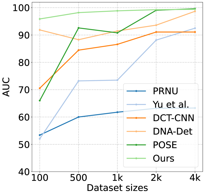
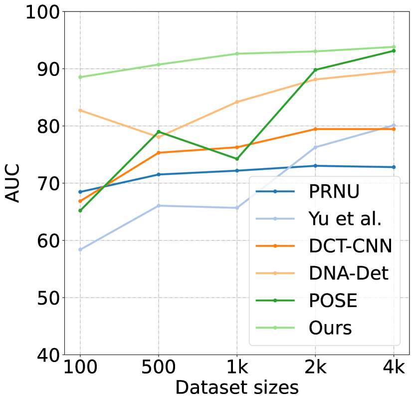
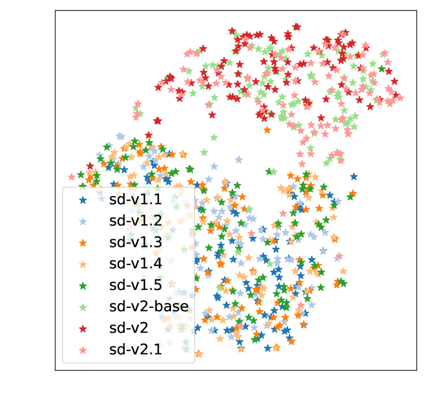
(a)

(b)

(c)

Figure 8: (a)(b) Open-set model identification accuracy and closed/open discrimination AUC along with dataset sizes. (c) Feature space visualization for different versions of stable diffusion models.

Model lineage analysis. Our fingerprint extractor also shows potential in analyzing the lineage between different versions of models based on their generated images. In Fig. 8c, we visualize the extracted features of various versions of stable diffusion models. The versions include sd-v1.1, v1.2, v1.3, v1.4, v2-base, v2, and v2.1. We can observe that the feature spaces of v1.# versions and v2.# versions overlap respectively. This alignment of feature spaces is consistent with the description of the relationship between these versions on the public website. Specifically, v1.2, v1.3, and v1.4 are resumed from v1.1, while v2 and v2.1 are resumed from v2-base.

6 Conclusions and future work

By analyzing generative network components in the frequency domain, we make the first attempt to identify sources for fingerprints of generative models. Utilizing the gained priors in a simulation strategy, we consequently improve the generality of fingerprint extraction in a range of model attribution scenarios. Our work opens the door to improving model fingerprint extraction based on synthetic data. For future works, it is promising to model the complexity and diversity of model fingerprints more accurately while balancing computational costs.

Appendix A Extra analysis of frequential fingerprint

A.1 Upsampling

Derivation for spectrum replication. In Fig. 3(b) of the main text, we observe that zero-interleaving in the spatial domain leads to spectrum replication in the frequency domain. We can derive this phenomenon as follows. Consider a 2D image signal $I\in\mathbb{R}^{M\times N}$, the 2D discrete Fourier transform for $I$ is denoted by:

$$F(u,v)=\sum_{x=0}^{M-1}\sum_{y=0}^{N-1}I(x,y)\cdot e^{-i2\pi(ux/M+vy/N)},$$ (5)

for $u=0,1,,2,\dots,M-1$ and $v=0,1,,2,\dots,N-1$. When we apply the ZeroInter function to $I$, which interleaves the input image with zeros and increases the spatial resolution by a factor of 2, denoted as $\hat{I}$, we have $\hat{I}(x,y)=0$ when $x$ or $y$ is odd. Consequently, we obtain:

$$\hat{F}(u,v) =\sum_{x=0}^{2M-1}\sum_{y=0}^{2N-1}\hat{I}(x,y)\cdot e^{-i2\pi(ux/2M+vy/2N)}$$ (6)

$$=\sum_{x=0}^{M-1}\sum_{y=0}^{N-1}\hat{I}(2x,2y)\cdot e^{-i2\pi(2ux/2M+2vy/2N)},$$

for $u=0,1,,2,\dots,2M-1$ and $v=0,1,,2,\dots,2N-1$. Then, we could derive the following equation:

$$\hat{F}(u+M,v+N) =\sum_{x=0}^{M-1}\sum_{y=0}^{N-1}\hat{I}(2x,2y)\cdot e^{-i2\pi(2(u+M)x/2M+2(v+N)y/2N)}$$ (7)

$$=\sum_{x=0}^{M-1}\sum_{y=0}^{N-1}\hat{I}(2x,2y)\cdot e^{-i2\pi(2ux/2M+2vy/2N)}\cdot e^{-i2\pi(x+y)}$$

$$=\sum_{x=0}^{M-1}\sum_{y=0}^{N-1}\hat{I}(2x,2y)\cdot e^{-i2\pi(2ux/2M+2vy/2N)}$$

$$=\hat{F}(u,v)$$

for $u=0,1,,2,\dots,M-1$ and $v=0,1,,2,\dots,N-1$. Similarly, $\hat{F}(u+M,v)=\hat{F}(u,v)$, and $\hat{F}(u,v+N)=\hat{F}(u,v)$. The equivalence relationship results in duplication of the spectrum.

Discussion on some empirical observations. About the relationship between generation artifacts and upsampling type, existing works have some empirical observations: Recent works [24; 25] have found that the Up+Conv form of upsampling produces fewer artifacts compared to deconvolution. Chandrasegaran et al. [14] empirically show that the high-frequency discrepancy of fake images can be avoided by a minor architecture change in the last upsampling operation,  i.e., change deconvolution to nearest or bilinear upsampling. Schwarz et al. [16] draw the conclusion that bilinear and nearest neighbor upsampling bias the generator towards predicting little high-frequency content. These studies collectively demonstrate that the utilization of nearest and bilinear interpolation leads to a reduction in the high-frequency components present in the generated images. This phenomenon can be understood by referring to Fig.3(c) in the main text, where it is evident that nearest and bilinear interpolation introduce frequency attenuation as a result of their implementation of low-pass upsampling filters.

A.2 Normalization and nonlinear activation functions

Normalization in the frequency domain. We mention in the main text that Normalization in the frequency domain has exactly the same form as the time domain. We can derive this conclusion as follows. Let $\mathbf{B}=\{x_{1},x_{2},...,x_{S}\}$ be a training mini-batch with batch size $S$, the basic procedure of Batch Normalization contains two steps:

$$\hat{x}_{i}=\frac{x_{i}-\mu_{\mathbf{B}}}{\sqrt{\sigma_{\mathbf{B}}^{2}+\epsilon}},i=1,\ldots,S$$ (8)

$$BNT_{\gamma,\beta}(x_{i})=\gamma\hat{x}_{i}+\beta,i=1,\ldots,S$$ (9)

where $\mu_{\mathbf{B}}$ and $\sigma_{\mathbf{B}}$ are mean and variance caculated over the mini-batch $\mathbf{B}$. $\gamma$ and $\beta$ are two learnable parameters for scaling and shifting the normalized feature map $\hat{x}_{i}$ in the first step. Based on the Discrete Fourier Transform, Batch normalization in the frequency domain could be described as follows [26]:

$$\mathcal{F}_{i}^{BNT}(u,v) =\sum_{x=0}^{H-1}\sum_{y=0}^{W-1}(\gamma\frac{I_{i}(x,y)-\mu_{\mathbf{B}}}{\sqrt{\sigma_{\mathbf{B}}^{2}+\epsilon}}+\beta)\cdot e^{-i2\pi(ux/H+vy/W)}$$ (10)

$$=\frac{\gamma}{\sqrt{\sigma_{\mathbf{B}}^{2}+\epsilon}}\sum_{x=0}^{H-1}\sum_{y=0}^{W-1}(I_{i}(x,y)-\mu_{\mathbf{B}})\cdot e^{-i2\pi(ux/H+vy/W)}+\sum_{x=0}^{H-1}\sum_{y=0}^{W-1}\beta\cdot e^{-i2\pi(ux/H+vy/W)}$$

$$=\gamma\frac{\mathcal{F}_{i}(u,v)-\sum_{x=0}^{H-1}\sum_{y=0}^{W-1}\mu_{\mathbf{B}}\cdot e^{-i2\pi(ux/H+vy/W)}}{\sqrt{\sigma_{\mathbf{B}}^{2}+\epsilon}}+\sum_{x=0}^{H-1}\sum_{y=0}^{W-1}\beta\cdot e^{-i2\pi(ux/H+vy/W)}$$

$$=\gamma\frac{\mathcal{F}_{i}(u,v)-\mu_{\mathcal{F},\mathbf{B}}}{\sqrt{\sigma_{\mathbf{B}}^{2}+\epsilon}}+\beta_{\mathcal{F}},$$

where $\mu_{\mathcal{F},\mathbf{B}}$ and $\beta_{\mathcal{F}}$ are two constants obtained by transforming $\mu_{\mathbf{B}}$ and $\beta$ to the frequency domain. Based on the formulation, we can learn that the implementation of Batch Normalization in the frequency domain has exactly the same form as the time domain, which normalizes, shifts, and scales the frequency spectrum of the input signal. Instance Normalization (IN) and Batch Normalization (BN) have the same computational form, except that the mean and variance are derived from an instance instead of a batch. Thus the formulation also applies to IN.

(a) Conv Spectrum

(b) None

(c) BN

(d) IN

(e) ReLU

(f) Sigmoid

(g) Tanh

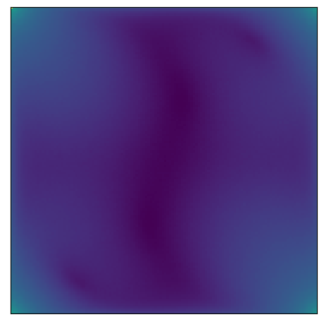
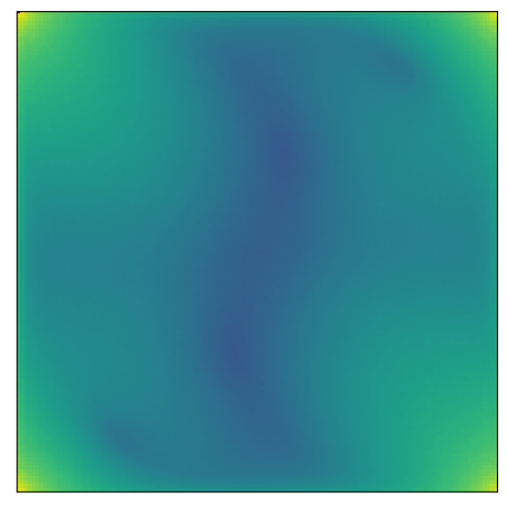
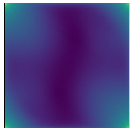
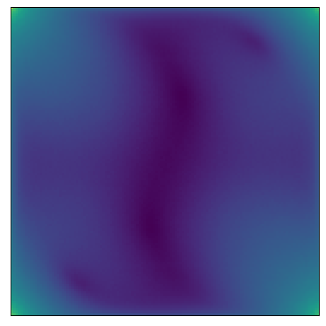
Figure 9: Visualize the effect of normalization and activation functions on frequency pattern.

Visualize the effect of normalization and activation function. Fig. 9 presents the visualization of the averaged spectrum for images generated by Conv+Norm/Activation blocks. The "Norm" component can be batch normalization or instance normalization, while the "Activation" component can be ReLU, Sigmoid, or Tanh. These blocks share a common Conv’ layer. Fig. 9(a) displays the spectrum of the ‘Conv’ layer, while Fig. 9(b) depicts the averaged spectrum of images directly output by the "Conv" layer. From the figure, we could observe that the normalization and activation functions have the potential to enhance or diminish the frequency pattern introduced by the convolution layer.

A.3 Frequency pattern attenuation over generative blocks

High-frequency component variation curve. In Fig.4(h) of the main text, we plot high-frequency component variation throughout the generation process. X-axis means every network component in the sequence of generation, and y-axis means the proportion of high frequencies of feature maps output by each network component. In the following, we detail the calculation process of values on the y-axis. Consider a 2D feature map $I\in\mathbb{R}^{M\times N}$ output by a certain component on the x-axis, the 2D discrete Fourier transform for $I$ is denoted by:

$$F(u,v)=\sum_{x=0}^{M-1}\sum_{y=0}^{N-1}I(x,y)\cdot e^{-i2\pi(ux/M+vy/N)},$$ (11)

Applying azimuthal integration over radial frequencies $\phi$, we get:

$$AI\left(\omega_{k}\right)=\int_{0}^{2\pi}\left\|F\left(\omega_{k}\cdot\cos(\phi),\omega_{k}\cdot\sin(\phi)\right)\right\|^{2}\mathrm{~{}d}\phi,$$ (12)

where $k=0,\ldots,M/2-1$. As seen, $AI(\omega_{k})$ is a simple but characteristic 1D representation of the 2D Fourier power spectrum, and each value is the radial integral over the 2D spectrum at a radius. Then we calculate of the high-frequency proportion as the sum of values in the latter half of $AI(\omega_{k})$ to the sum of all values:

$$HP\_ratio=\frac{\sum_{k=M/4}^{M/2-1}AI\left(\omega_{k}\right)}{\sum_{k=0}^{M/2-1}AI\left(\omega_{k}\right)}$$ (13)

Appendix B Dataset

For the model verification experiment, we randomly selected 10,000 pairs of images from the generated images of the models listed in Tab.1 of the main text. These pairs consisted of 5,000 negative pairs and 5,000 positive pairs. Each pair included two groups of images, with each group containing $N_{S}$ images. Images in positive pairs originate from the same model, while the group of images in negative pairs are sourced from different models.

For the open-set model identification experiment, the training sample size for each known model varied, including 100, 500, 1000, 2000, and 5000 samples, as depicted in Fig. 8 of the main text. The testing set consists of 1000 non-overlapping samples per known model, and there are 1000 samples for each unknown model.

Appendix C Experiment

C.1 Implementation details

In our experiment, we set the batch size to 200. For each image in a batch, we randomly select a model from the model pool and transform the input image into a fingerprinted image. The learning rate for the fingerprint extractor is set to $1e^{-4}$. We employ a margin of 0.3 for the triplet loss and assign equal weights of 1 to both the triplet loss and classification loss. Additionally, we utilize a step schedule with a gamma value of 0.9 and a step size of 100.

C.2 Transferability to Transformer-based generative models

While our analysis and data synthesis strategy primarily focuses on CNN-based generative models, we observe that the transferability of our pre-trained fingerprint extractor extends to transformer-based generative models as well. Specifically, we consider seven transformer-based face generators in the additional evaluation: Gansformer_ffhq256 [49], StyleSwin_ffhq256 [50], StyleSwin_celeba256, Styleformer_celeba64 [51], TransGAN_celeba64 [52], StyleSwin_celeba1024, and StyleSwin_ffhq1024. The suffix "_ffhq256" indicates that the models were trained on the FFHQ dataset with a resolution of 256 for instance.

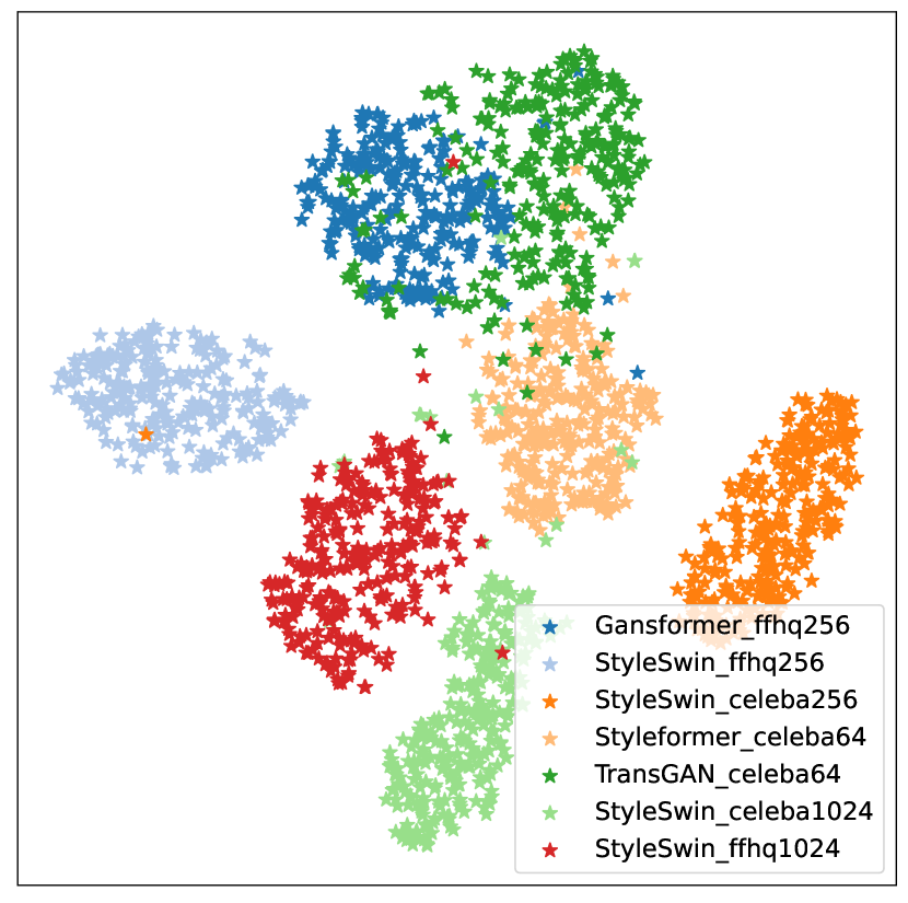
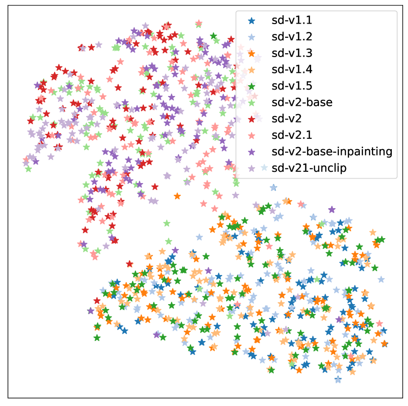
(a)

(b)

Figure 10: (a) Feature visualization on transformer-based generative models. (b) Feature visualization on different versions of stable diffusion models

As depicted in Fig. 10(a), our pre-trained fingerprint extractor effectively captures unique fingerprints from these models, even without being trained on any images specifically from transformer-based models. This showcases the transferability of our pre-trained model to novel model types in the open world, encompassing transformer-based generative models. To delve into the underlying factors contributing to this transferability, we conduct an analysis of the architectures of these models. Through the analysis, we observe that while transformer-based models primarily utilize transformer blocks as generative components, they also incorporate convolution or upsampling layers during the generation process. For instance, StyleSwin and Styleformer employ convolution layers to transform features from transformer blocks to RGB images. Gansformer incorporates standard convolution and upsampling after the self-attention layer. TransGAN does not utilize convolution during generation but incorporates interpolation-based upsampling layers. In future research, it would be valuable to investigate the impact of self-attention layers on frequency patterns and explore their influence in greater detail.

C.3 More model lineage result on Stable Diffusion models

In the main text, we present visualizations of the feature space for various versions of stable-diffusion models for Text2Image generation. Due to their visual modeling capabilities, they can also be fine-tuned for downstream tasks with few training steps, such as unclip and inpainting in Fig. 11. We additionally include the feature visualization results for the two models in Fig. 10(b). As seen, the downstream models could be correctly attributed as being derived from stable-diffusion v2 models based on the high similarity of their features.

original image

unclipped image

original image

mask image

inpainted image

|

(a)

(b)

Figure 11: (a) Stable-diffusion-2-1-unclip. (b) Stable-diffusion-2-inpainting.

Appendix D Limitations and Future Work

In this paper, we make the first attempt to provide empirical explanations for generative model fingerprints in the frequency domain and derive a data synthesis strategy for more generalized fingerprint extraction in the open world. While our method generates compelling results. It is not without limitations. Firstly, inspired by the frequency pattern attenuation phenomenon, we propose to simulate diverse frequency patterns based on generative blocks. Despite the superior transferability and time efficiency, the complex fingerprints from previous blocks may not be simulated sufficiently. In the future, it is worthwhile to further narrow the gap between simulated fingerprints and fingerprints of real generative models while balancing computation costs. Second, our analysis mainly focuses on CNN-based generative models. Although the pre-trained fingerprint extractor shows superior transferability to transformer-based models, it’s also worthwhile to study the impact of self-attention layers on frequency patterns for further work, given the successful applications of transformer blocks into generative models. Last, with the drawn observations in this paper, model fingerprints in the high-frequency components could be removed by model stealers. How to design defenses for these attacks remains an open problem. Overall, our research provides valuable insights and techniques for generative model fingerprint extraction, there are several areas for future improvement, including enhancing the realism of simulated fingerprints, studying the impact of self-attention layers, and addressing attacks related to fingerprint removal.

References

- [1] Nichol, A., P. Dhariwal, A. Ramesh, et al. Glide: Towards photorealistic image generation and editing with text-guided diffusion models. In ICML. 2021.
- [2] Ramesh, A., P. Dhariwal, A. Nichol, et al. Hierarchical text-conditional image generation with clip latents. arXiv preprint arXiv:2204.06125, 2022.
- [3] Rombach, R., A. Blattmann, D. Lorenz, et al. High-resolution image synthesis with latent diffusion models. In CVPR. 2022.
- [4] Midjourney. https://www.midjourney.com.
- [5] Marra, F., D. Gragnaniello, L. Verdoliva, et al. Do gans leave artificial fingerprints? In MIPR. 2019.
- [6] Yu, N., L. S. Davis, M. Fritz. Attributing fake images to gans: Learning and analyzing gan fingerprints. In ICCV. 2019.
- [7] Xuan, X., B. Peng, W. Wang, et al. Scalable fine-grained generated image classification based on deep metric learning. arXiv preprint arXiv:1912.11082, 2019.
- [8] Yang, T., Z. Huang, J. Cao, et al. Deepfake network architecture attribution. In AAAI. 2022.
- [9] Bui, T., N. Yu, J. Collomosse. Repmix: Representation mixing for robust attribution of synthesized images. In ECCV. 2022.
- [10] Yang, T., D. Wang, F. Tang, et al. Progressive open space expansion for open-set model attribution. In CVPR. 2023.
- [11] Frank, J., T. Eisenhofer, L. Schönherr, et al. Leveraging frequency analysis for deep fake image recognition. In ICML. 2020.
- [12] Girish, S., S. Suri, S. S. Rambhatla, et al. Towards discovery and attribution of open-world gan generated images. In ICCV. 2021.
- [13] Liu, Z., P. Luo, X. Wang, et al. Deep learning face attributes in the wild. In ICCV. 2015.
- [14] Chandrasegaran, K., N.-T. Tran, N.-M. Cheung. A closer look at fourier spectrum discrepancies for cnn-generated images detection. In CVPR. 2021.
- [15] Durall, R., M. Keuper, J. Keuper. Watch your up-convolution: Cnn based generative deep neural networks are failing to reproduce spectral distributions. In CVPR. 2020.
- [16] Schwarz, K., Y. Liao, A. Geiger. On the frequency bias of generative models. In NeurIPS. 2021.
- [17] Dzanic, T., K. Shah, F. Witherden. Fourier spectrum discrepancies in deep network generated images. In NeurIPS. 2020.
- [18] Khayatkhoei, M., A. Elgammal. Spatial frequency bias in convolutional generative adversarial networks. In AAAI. 2022.
- [19] Yu, N., V. Skripniuk, D. Chen, et al. Responsible disclosure of generative models using scalable fingerprinting. In ICLR. 2022.
- [20] Yu, N., V. Skripniuk, S. Abdelnabi, et al. Artificial gan fingerprints: Rooting deepfake attribution in training data. In ICCV. 2021.
- [21] Kim, C., Y. Ren, Y. Yang. Decentralized attribution of generative models. In ICLR. 2021.
- [22] Oppenheim, A. V. Discrete-time signal processing. Pearson Education India, 1999.
- [23] Karras, T., S. Laine, M. Aittala, et al. Analyzing and improving the image quality of stylegan. In CVPR. 2020.
- [24] Odena, A., V. Dumoulin, C. Olah. Deconvolution and checkerboard artifacts. Distill, 1(10), 2016.
- [25] Wojna, Z., V. Ferrari, S. Guadarrama, et al. The devil is in the decoder: Classification, regression and gans. IJCV, 127(11):1694–1706, 2019.
- [26] Pan, H. Learning convolutional neural networks in frequency domain. arXiv preprint arXiv:2204.06718, 2022.
- [27] Ayat, S. O., M. Khalil-Hani, A. A.-H. Ab Rahman, et al. Spectral-based convolutional neural network without multiple spatial-frequency domain switchings. Neurocomputing, 364:152–167, 2019.
- [28] Karras, T., M. Aittala, S. Laine, et al. Alias-free generative adversarial networks. In NeurIPS. 2021.
- [29] Karras, T., T. Aila, S. Laine, et al. Progressive growing of gans for improved quality, stability, and variation. In ICLR. 2018.
- [30] Bińkowski, M., D. J. Sutherland, M. Arbel, et al. Demystifying MMD GANs. In ICLR. 2018.
- [31] Zhang, H., I. Goodfellow, D. Metaxas, et al. Self-attention generative adversarial networks. In ICML. 2019.
- [32] Lee, K. S., N.-T. Tran, N.-M. Cheung. Infomax-gan: Improved adversarial image generation via information maximization and contrastive learning. In WACV. 2021.
- [33] Choi, Y., M. Choi, M. Kim, et al. Stargan: Unified generative adversarial networks for multi-domain image-to-image translation. In CVPR. 2018.
- [34] He, Z., W. Zuo, M. Kan, et al. Attgan: Facial attribute editing by only changing what you want. TIP, 28(11):5464–5478, 2019.
- [35] Karras, T., S. Laine, T. Aila. A style-based generator architecture for generative adversarial networks. In CVPR. 2019.
- [36] Brock, A., J. Donahue, K. Simonyan. Large scale GAN training for high fidelity natural image synthesis. In ICLR. 2019.
- [37] Lučić, M., M. Tschannen, M. Ritter, et al. High-fidelity image generation with fewer labels. In ICML. 2019.
- [38] Kang, M., J. Park. Contragan: Contrastive learning for conditional image generation. In NeurIPS. 2020.
- [39] Kingma, D. P., M. Welling. Auto-encoding variational bayes. In ICLR. 2014.
- [40] Higgins, I., L. Matthey, A. Pal, et al. beta-vae: Learning basic visual concepts with a constrained variational framework. In ICLR. 2017.
- [41] Burgess, C. P., I. Higgins, A. Pal, et al. Understanding disentangling in beta-vae. In NIPS workshop. 2017.
- [42] Zhao, S., J. Song, S. Ermon. Infovae: Information maximizing variational autoencoders. arXiv preprint arXiv:1706.02262, 2017.
- [43] Kingma, D. P., P. Dhariwal. Glow: Generative flow with invertible 1x1 convolutions. In NeurIPS. 2018.
- [44] Chen, R. T., J. Behrmann, D. K. Duvenaud, et al. Residual flows for invertible generative modeling. In NeurIPS. 2019.
- [45] Dhariwal, P., A. Nichol. Diffusion models beat gans on image synthesis. In NeurIPS. 2021.
- [46] Ho, J., A. Jain, P. Abbeel. Denoising diffusion probabilistic models. In NeurIPS. 2020.
- [47] Liu, L., Y. Ren, Z. Lin, et al. Pseudo numerical methods for diffusion models on manifolds. In ICLR. 2022.
- [48] Dall-e mini. https://github.com/borisdayma/dalle-mini.
- [49] Hudson, D. A., L. Zitnick. Generative adversarial transformers. In ICML. 2021.
- [50] Zhang, B., S. Gu, B. Zhang, et al. Styleswin: Transformer-based gan for high-resolution image generation. In CVPR. 2022.
- [51] Park, J., Y. Kim. Styleformer: Transformer based generative adversarial networks with style vector. In CVPR. 2022.
- [52] Jiang, Y., S. Chang, Z. Wang. Transgan: Two pure transformers can make one strong gan, and that can scale up. In NeurIPS. 2021.