Fast Searching The Densest Subgraph And Decomposition With Local Optimality

Abstract

Densest Subgraph Problem (DSP) is an important primitive problem with a wide range of applications, including fraud detection, community detection, and DNA motif discovery. Edge-based density is one of the most common metrics in DSP. Although a maximum flow algorithm can exactly solve it in polynomial time, the increasing amount of data and the high complexity of algorithms motivate scientists to find approximation algorithms. Among these, its duality of linear programming derives several iterative algorithms including Greedy++, Frank-Wolfe, and FISTA which redistribute edge weights to find the densest subgraph, however, these iterative algorithms vibrate around the optimal solution, which is not satisfactory for fast convergence. We propose our main algorithm Locally Optimal Weight Distribution (Lowd) to distribute the remaining edge weights in a locally optimal operation to converge to the optimal solution monotonically. Theoretically, we show that it will reach the optimal state of specific quadratic programming, which is called locally-dense decomposition. Besides, we show that it is not necessary to consider most of the edges in the original graph. Therefore, we develop a pruning algorithm using a modified Counting Sort to prune graphs by removing unnecessary edges and nodes, and then we can search the densest subgraph in a much smaller graph.

I Introduction

Finding subgraphs with the highest average degrees in large networks is an important primitive problem in data mining, and has been applied to different areas including social networks [1], biological analysis [2], traffic pattern mining [3], and graph database [4, 5]. The maximum-flow-based algorithm [6] can exactly solve DSP by utilizing the binary search in polynomial time, which is ill-suited for large graphs due to the prohibitive cost. The greedy-peeling algorithm (‘Greedy’ as an abbreviation) proposed by Charikar [7] can provide a $1/2$-approximation guaranteed solution in linear time by greedily deleting the nodes with the minimum degree. There are also various variants for both the exact and approximation algorithms applied to different scenarios.

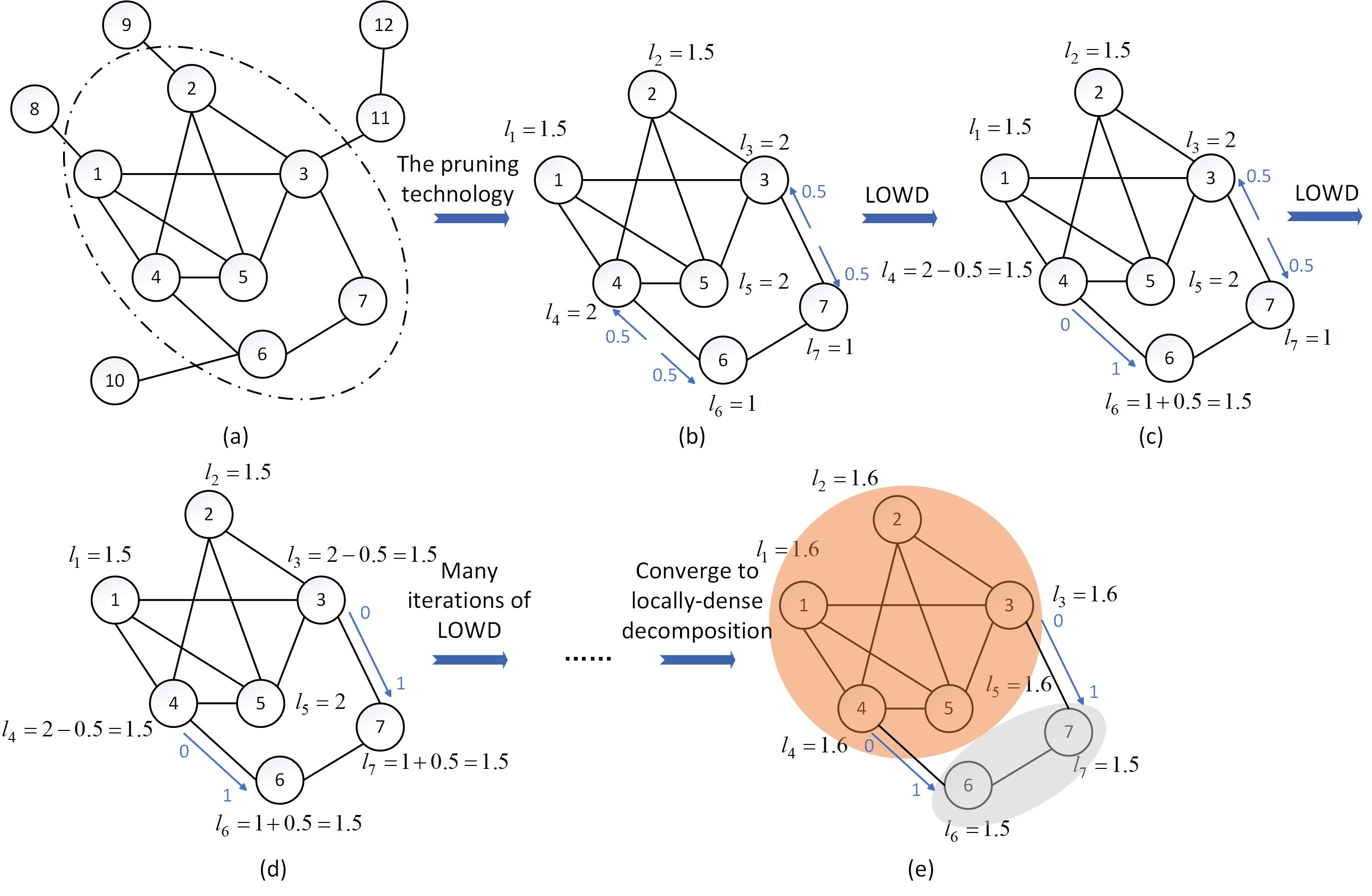
Figure 1: An example of our methods. $(a)\to(b)$: Remove some nodes using our pruning technique. $(b)$: Initialize node loads by distributing edge weight equally to two endpoints. $(b)\to(c)$: distribute the weight of the edge connecting nodes 4 and 6 to node 6 in one-way. $(c)\to(d)$: distribute the weight of the edge connecting nodes 3 and 7 to node 7 in one-way. $(d)\to(e)$: After many iterations of Lowd, the graph converges into the locally dense decomposition, that is, loads of nodes 1, 2, 3, 4, and 5 gradually become equal through the redistribution of edge loads and form a nodeset. Nodes 6 and 7 form a nodeset, and edges between two different nodesets are undirectionally distributed from the nodeset with a higher load to the nodeset with a lower node load. And deleting the node with the lowest load one by one can find the densest subgraph, that is, the subgraph consisting of nodes 1, 2, 3, 4, and 5. The order in which edges are selected during edge weight redistribution does not affect the result.

In addition, to detect the densest subgraph more efficiently, in recent years, many DSP algorithms and discoveries towards its dual linear programming (LP) are developed, which was first introduced in [7]. E.g., Danisch et al. [8] redistribute edge weights based on the Frank-Wolfe algorithm, [9] relaxes the constraints of LP dual and proposes an algorithm for dynamic graphs, Greedy++ was proposed in [10] based on the multiplicative weights update (MWU) framework, which iteratively implements Greedy to search the densest subgraph. In [11], it gives a theoretical guarantee to the relationship between iteration count and approximation ratio of Greedy++, and popularizes Greedy++ to super-modular function $f(S)$, i.e., the definition of density is $\frac{f(S)}{|S|}$. Besides, [12] proposes FISTA algorithm with a faster convergence speed than Greedy++. Frank-Wolfe, Greedy++, and FISTA are all developed based on classical methods towards convex optimization, like gradient descent and MWU. However, these iterative methods will vibrate around the optimal solution, which is time-consuming.

In this paper, We elaborately design a novel algorithm called locally optimal weight distribution (Lowd) algorithm, based on the dual problem of LP for DSP using a locally optimal operation with monotonic convergence to the optimal value, it detects the densest subgraph more efficiently than previous studies. Besides, we develop a pruning technology to remove most nodes that don’t belong to the densest subgraph before using Lowd to detect the densest subgraph. Some pruning technique is used in [17] but we use a modified Counting Sort to make our pruning comply with linear time complexity on unweight graphs, we also prove that our pruning technique is a subprocess of Greedy. In addition, we theoretically prove that Lowd converges to the locally-dense decomposition solution, which is a well-studied problem [13, 14, 8, 12, 15, 16]. The locally-dense decomposition consists of a set of subgraphs with nested structures and densities. Such decomposition can be derived by various iterative methods, including Frank-Wolfe, Greedy++, and FISTA.

Moreover, we comprehensively verify the performance of Lowd over 26 real-world networks. The experimental results show that Lowd has a better convergence rate than other iterative algorithms, i.e., Frank-Wolfe, Greedy++, and FISTA, when detecting the densest subgraph and locally-dense decomposition.

In Figure 1, we illustrate an example of Lowd algorithm, and the final locally-dense decomposition. First, we use the pruning technique to delete unnecessary nodes in $(a)$. In the initial state of Lowd, we distribute each edge weight equally to endpoints, accumulating it as the node loads on the endpoints. Then, Lowd redistributes edge weights to minimize the difference between two endpoints’ loads, for example, in $(b)$ and $(c)$, node 4 with load 2 transits edge weight to node 6 with load 1, and their loads both become 1.5, a similar scenario happens on nodes 5 and 7. Therefore, in order to make node loads more balanced, a node with a higher load should transit edge weight to its neighbors with lower loads. From a global perspective, edge weight should be redistributed from nodes with higher loads to nodes with lower loads in iterations, and the densest subgraph can be easily discovered by deleting the node with the lowest load one by one. And the graph finally converges to the locally-dense decomposition like $(e)$.

In summary, our main contributions include as follows:

• We propose an iterative mining method called Lowd for DSP according to its LP dual and prove it will converge into the locally-dense decomposition, which is a variant of DSP. We also exhibit how Lowd solves both problems in a locally optimal operation iteratively.

• We develop a pruning technique to lock the densest subgraph into a graph with a much smaller size using a modified Counting Sort and prove that it is a subprocess of Greedy search.

• We did sufficient experiments on 26 real-world datasets in various fields, with sizes up to hundreds of millions of edges. Our result shows that Lowd can detect the densest subgraph much faster than other baselines and it can converge to the locally-dense decomposition more efficiently, while the pruning technique as a pre-process can effectively reduce the computation.

Organization. We organize the rest paper as below. In section II we present two problems formally: the densest subgraph problem and the locally-dense decomposition problem. In section III we proposes an iterative method to deal with the linear programming of DSP and quadratic programming of locally-dense decomposition, and develop a pruning technique to lock the densest subgraph into a much smaller graph. We exhibit their efficient performance based on various experiments in section IV. In section V we review the related work about DSP and its variants. We summarize our work and make a prospect for future work In section VI.

Due to space limits, part of the theorems, lemmas, and experimental results are given in the appendix.

II preliminaries

TABLE I: Symbols and Definitions.

Symbol	Definition and Description
$\mathcal{G}(\mathcal{V},\mathcal{E},\mathcal{W})$	Graph $\mathcal{G}$ with nodeset $\mathcal{V}$, Edgeset $\mathcal{E}$ and edge weights $\mathcal{W}$
$M$,$N$	Number of edges and nodes of a graph
$\mathcal{S}$	Subset of nodes, i.e., $\mathcal{S}\subseteq\mathcal{V}$
$\mathcal{S}^{*}$	The nodeset of the densest subgraph
$\mathcal{E}(\mathcal{S}),\mathcal{W}(\mathcal{S})$	the edgeset and total weights induced by $\mathcal{S}$
$\rho\left(\mathcal{S}\right)$	The density of the nodeset $\mathcal{S}$
$\rho^{*}$	The density of the densest subgraph
$\mathrm{d}_{\mathcal{S}}(u)$	The degree of node $u$ in $\mathcal{S}$
$l_{u},w_{e}$	Load of the node $u$ and Weight of the edge $e$
$f_{e}(u)$	The weight distributed to node $v$ from edge $e$

In this section, we formally define the densest subgraph detection and locally-dense decomposition problem that we focus on. Table I summarizes the main symbols used in the paper.

Let $\mathcal{G}=(\mathcal{V},\mathcal{E},\mathcal{W})$ be an undirected graph with $N=|\mathcal{V}|$ vertices and $M=|\mathcal{E}|$ edges. For any $e\in\mathcal{E}\subseteq\mathcal{V}\times\mathcal{V}$, its weight is $w_{e}\in\mathcal{W}$ with $w_{e}\in\mathbb{R}_{+}$ and $w_{e}=1$ for the weighted and unweighted graph, respectively. Given a node subset $\mathcal{S}\subseteq\mathcal{V}$, $\mathcal{E}(\mathcal{S})$ denotes the set of edges and $\mathcal{W}(\mathcal{S})$ denotes the total weights induced by $\mathcal{S}$, and $\mathrm{d}_{\mathcal{S}}(u)$ is the degree of $u$ in the induced subgraph, i.e., the total weights of edges connected to $u$ within the set $\mathcal{S}$. Bold letters are used to represent vectors.

Given the nodeset $\mathcal{S}$, the edge density of the subgraph $\mathcal{G}(\mathcal{S})$ is defined as

$$\rho(\mathcal{S})\coloneqq\frac{\mathcal{W}(\mathcal{S})}{|\mathcal{S}|}=\frac{\sum_{u\in\mathcal{S}}\mathrm{d}_{\mathcal{S}}(u)}{2\cdot|\mathcal{S}|}.$$

Accordingly, we present the formal definition of the densest subgraph problem as below:

Problem 1 (Densest Subgraph Problem (DSP)).

Given an undirected graph $\mathcal{G}=(\mathcal{V},\mathcal{E},\mathcal{W})$, find the subset of nodes $\mathcal{S}^{*}$ such that $\mathcal{S}^{*}=\operatorname*{arg\,max}_{\mathcal{S}\subseteq\mathcal{V}}\rho(\mathcal{S})$.

Another variant of DSP is more general, which is called locally-dense decomposition.

Definition 1 (Locally-Dense Decomposition (LDD) [14, 16]).

Given an undirected graph $\mathcal{G}=(\mathcal{V},\mathcal{E},\mathcal{W})$, it has a nested decomposition consisting of a sequence $\emptyset=B_{0}\subsetneqq B_{1}\subsetneqq\ldots\subsetneqq B_{k}=\mathcal{V}$. We define $B_{i}$ as the maximal densest subgraph properly containing $B_{i-1}$, that is,

$$B_{i}=\operatorname*{arg\,max}_{{S\supsetneqq B_{i-1}}}{\frac{\mathcal{W}(S)-\mathcal{W}(B_{i-1})}{|S\setminus B_{i-1}|}}$$

As we can see, DSP is a sub-problem of locally-dense decomposition, because $B_{1}$ is the maximal densest subgraph of the whole graph $\mathcal{G}$, corresponding to the target in Problem 1. LDD is also closely related to convergence analysis for iterative update methods towards DSP [8, 10, 12]. Formally, the locally-dense decomposition problem over $\mathcal{G}$ is formulated as:

Problem 2 (Locally-dense decomposition Problem[14, 16, 8]).

Given an undirected graph $\mathcal{G}=(\mathcal{V},\mathcal{E},\mathcal{W})$, find its locally-dense decomposition $\emptyset=B_{0}\subsetneqq B_{1}\subsetneqq\ldots\subsetneqq B_{k}=\mathcal{V}$.

Based on the above problem definition, we summarize some important properties of LDD.

Property 1 ([8]).

Given an undirected graph $\mathcal{G}=(\mathcal{V},\mathcal{E},\mathcal{W})$, its locally-dense decomposition is unique.

Property 2 ([12]).

And for any $u\in B_{i}$, let

$$\lambda_{u}=\lambda_{i}\coloneqq{\frac{\mathcal{W}(\mathcal{E}(W))-\mathcal{W}(\mathcal{E}(B_{i-1}))}{|W\setminus B_{i-1}|}},$$

there is a unique optimal $\bm{\ell}^{*}$ so that ${\ell_{v}}^{*}=\lambda_{v}$ for each node $v$. And $\lambda_{1}>\lambda_{2}>...>\lambda_{k}$.

Property 3 ([8, 15]).

For an optimal solution $(\bm{f}^{*},\bm{\ell}^{*})$, if there is an edge $e=(v_{1},v_{2})$ with ${\ell_{v_{1}}}^{*}>{\ell_{v_{2}}}^{*}$, then ${f_{e}}^{*}(v_{1})=0$.

Properties 1 and 2 imply that in the unique locally-dense decomposition, each node in set $B_{i}\setminus B_{i-1}$ has the same load $\lambda_{i}$, and the nodeset in the inner nodeset in the inner layer is denser than one in the outer layer. Property 3 means the weight of edge e connecting two layers should be only distributed to the node with a lower load in one-way.

In section III we will introduce an algorithm which provides an iterative operation to solve both DSP and locally-dense decomposition problem.

III methodology

Input: Undirected graph $\mathcal{G}$, iteration count $T$.

Output: An approximately densest subgraph of $\mathcal{G}$.

1 for $e=(u,v)\in\mathcal{E}$ do

2       $f_{e}(u)=f_{e}(v)=\frac{w_{e}}{2}$; $\triangleright$ initialize edge weight

3for $u\in\mathcal{V}$ do

4       $\ell_{u}=\sum_{e\in\mathcal{E}:u\in e}{f_{e}(u)}$ $\triangleright$ initialize node load

5for $k:1\to T$ do

6       for $e=(u,v)\in\mathcal{E}$ do

7             if $\ell_{u}>\ell_{v}$ then

8                   $\triangleright$ balance nodes loads as much as possible

9                  $d\leftarrow\min\{(\ell_{u}-\ell_{v})/2,\,f_{e}(u)\}$;

10                  $\ell_{u}\leftarrow\ell_{u}-d$;

11                  $f_{e}(u)\leftarrow f_{e}(u)-d$;

12                  $\ell_{v}\leftarrow\ell_{v}+d$;

13                  $f_{e}(v)\leftarrow f_{e}(v)+d$;

14            else

15                   $d\leftarrow\min\{(\ell_{v}-\ell_{u})/2,\,f_{e}(v)\}$;

16                  $\ell_{u}\leftarrow\ell_{u}+d$;

17                  $f_{e}(u)\leftarrow f_{e}(u)+d$;

18                  $\ell_{v}\leftarrow\ell_{v}-d$;

19                  $f_{e}(v)\leftarrow f_{e}(v)-d$;

20            

21      

22$\mathcal{S}^{*},\mathcal{S}\leftarrow\mathcal{V},\mathcal{V}$; $\triangleright$ sort $l_{u}$ in a non-decreasing order

23$V_{s}\leftarrow\operatorname*{arg\,sort}_{u\in\mathcal{V}}l_{u}$;

24for $i:1\to N$ do

25       $\mathcal{S}\leftarrow\mathcal{S}\setminus\{\mathcal{V}_{s}(i)\}$; $\triangleright$ $\mathcal{V}_{s}(i):$ the $i$-th element of $\mathcal{V}_{s}$

26      if $\rho(\mathcal{S}^{*})<\rho(\mathcal{S})$ then

27             $\mathcal{S}^{*}\leftarrow\mathcal{S}$;

28      

return $\mathcal{G}(\mathcal{S}^{*})$.

Algorithm 1 Lowd: Locally optimal weight distribution for densest subgraph detection

In this section, through the lens of the primal-dual formulation of linear programming, we illustrate our idea for solving DSP and propose the locally optimal weight distribution algorithm, Lowd, which is a fast iterative approach to searching the densest subgraph according to the LP dual of DSP. We also theoretically prove that Lowd makes the graph converge into locally-dense decomposition. To search the densest subgraph more efficiently, we propose a pruning algorithm, rendering the necessary condition for DSP and corresponding to a subprocess of Greedy.

III-A Locally Optimal Weight Distribution Algorithm

Firstly we present the pseudo code of Lowd in algorithm 1 and explain it. In algorithm 1, given an undirected graph $\mathcal{G}$ and iteration count T, we distribute each edge $e$’s weight to its two endpoints $u$ and $v$ and use vector $\bm{f}$ to describe it. Specifically, $f_{e}(u)$ is the weight distributed to node $u$ from edge $e$. Besides, we use vector $\bm{\ell}$ to remark the load of each node received from all corresponding edges, specifically, $\ell_{u}=\sum_{e\in\mathcal{E}:u\in e}{f_{e}(u)}$. In lines 1-4, we distribute each edge equally to two endpoints as the initial state and accordingly calculate node loads. Its time complexity is $O(M)$. Lines 5-14 mean that it redistributes the weight of edge $e=(u,v)$ to minimize the difference of $\ell_{u}$ and $\ell_{v}$ for every $e\in\mathcal{E}$ in iterations. Its time complexity is $O(MT)$. In lines 7-10 we distribute more edge weight from $u$ to $v$, and update step $d$ is $(\ell_{u}-\ell_{v})/2$ if it will not make any $f_{e}(u)<0$, otherwise $d$ is $f_{e}(u)$. In lines 11-14 the circumstance is the opposite. In line 15 we set the whole nodeset as the initial nodeset $S$. In lines 16-20 we sort S according to node loads and delete the node with the lowest weight one by one to get a subgraph with high density, its time complexity is $O(M+NlogN)$.

Complexity 1.

The time complexity of Lowd is $O(MT+M+NlogN)$.

Remark. Although Lowd can detect the densest subgraph with enough iterations, but we cannot determine iteration count required. Therefore, our Lowd belongs to the approximation algorithm in strict terms because actually we just set the iteration count to get an approximate solution for DSP. The same circumstance happens on other approximation algorithms including Frank-Wolfe in [8], Greedy++ in [10] and FISTA in [12].

III-B Lowd converges to DSP solution

In order to figure out how Lowd searches the densest subgraph iteratively, we first introduce the LP primal-dual of DSP from [7, 10, 8] as follows. The notation of LP primal-dual is the same as [10].

maximize $$\sum_{e\in\mathcal{E}}{w_{e}y_{e}}$$ (1)

subject to $$y_{e}\leq x_{u},\qquad\forall e=uv\in\mathcal{E}$$

$$y_{e}\leq x_{v},\qquad\forall e=uv\in\mathcal{E}$$

$$\sum_{v\in\mathcal{V}}{x_{v}}\leq 1$$

$$y_{e}\geq 0\qquad\forall e\in\mathcal{E}$$

$$x_{v}\geq 0\qquad\forall v\in\mathcal{V}$$

In LP (1), the binary $x_{u}$ and $y_{e}$ indicate the contribution to density of the densest subgraph from node $u$ and edge $e$. The maximum of LP (1) is $\rho^{*}$, i.e., the maximum density in DSP. You can set $y_{e}=\frac{1}{\mathcal{S}^{*}}$ if $e\in\mathcal{E}(\mathcal{S}^{*})$ otherwise $y_{e}=0$ and set $x_{u}=\frac{1}{\mathcal{S}^{*}}$ if $u\in\mathcal{S}^{*}$ otherwise $x_{u}=0$, then you will get $\frac{\mathcal{W}(\mathcal{S}^{*})}{\mathcal{S}^{*}}$ as the optimal value of $\sum_{e\in\mathcal{E}}{w_{e}y_{e}}$. Instead of using the primal problem, we resort to the LP dual for DSP to illustrate our motivation:

minimize $$D$$ (2)

subject to $$f_{e}(u)+f_{e}(v)\geq w_{e}\qquad\forall e=uv\in\mathcal{E}$$

$$\ell_{v}\overset{\text{def}}{=}\sum_{e\ni v}{f_{e}(v)}\leq D\qquad\forall v\in\mathcal{V}$$

$$f_{e}(u)\geq 0\qquad\forall e=uv\in E$$

$$f_{e}(v)\geq 0\qquad\forall e=uv\in E$$

From strong duality, we know its optimal value is also $\rho^{*}$. The symbols in LP (2) can be interpreted in accordance with the description in Lowd. $f_{e}(u)$ and $f_{e}(v)$ should be both positive and the sum is not less than $w_{e}$ to ensure the edge is distributed thoroughly. Actually, in the LP dual of DSP, we can keep $f_{e}(u)+f_{e}(v)=w_{e}$ instead of $f_{e}(u)+f_{e}(v)\geq w_{e}$, because the former can keep constraint condition and doesn’t increase optimization objective $D$. Consequently, we can get the optimization objective $D$ with tighter constraint in LP (3) as below.

note: During the whole process we set $D=\max_{v\in\mathcal{V}}\ell_{v}$ to minimize it as much as possible.

minimize $$D$$ (3)

subject to $$f_{e}(u)+f_{e}(v)=w_{e}\qquad\forall e=uv\in\mathcal{E}$$

$$\ell_{v}=\sum_{e\ni v}{f_{e}(v)}\leq D\qquad\forall v\in\mathcal{V}$$

$$f_{e}(u)\geq 0\qquad\forall e=uv\in\mathcal{E}$$

$$f_{e}(v)\geq 0\qquad\forall e=uv\in\mathcal{E}$$

Intuitively speaking, what Lowd does is to redistribute each edge weight to minimize the difference between loads of two endpoints for each edge in iterations, i.e., propagate edge weights from nodes with higher loads to nodes with lower loads. And the impact of Lowd on LP (3) is that the node $v$ with the highest node load $l_{v}=D$ will decrease its weight because $v$ transits its edge weights to its neighbors. After experiencing some iterations, the highest node load will decrease gradually to some value, in fact, the value is the minimum of $D$, i.e., $\rho^{*}$. Formally we propose the following theorem:

Theorem 1.

The iterative operation in Lowd can make the sequence $\left\{D_{t}\right\}$ converge to $\rho^{*}$, where $D_{t}(t>0)$ means the optimization objective $D$ after $t$ iterations of Lowd and $D_{0}$ is the value in the initial state.

Next, we will give theoretical proofs for Theorem 1, first we need the following classical theorem for convergence.

Theorem 2 (Monotone Convergence Theorem [18]).

If the sequence $\left\{a_{n}\right\}$ has an upper bound and it is monotonically non-decreasing (or has a lower bound and it is monotonically non-increasing), then the sequence $\left\{a_{n}\right\}$ converges, i.e., a monotonically bounded sequence must have a limit.

Now that $\left\{D_{t}\right\}$ has a lower bound $\rho^{*}$ according to strong duality, and $\left\{D_{t}\right\}$ is monotonically non-increasing under Lowd’s iterative operation (because in the whole process Lowd just balances loads of two endpoints and it will not produce any new node with load higher than the optimization objective $D$). Then $D_{t}$ is non-increasing and it must converge to some value.

It is helpless for solving DSP if the optimization objective converges to some value which is not the minimum, i.e., $\rho^{*}$. However, we can use the following lemma to help to prove Theorem 1.

Lemma 1.

for $\forall t\in\mathbb{N}$, there must be $D_{t+N}<D_{t}$ if $D_{t}\neq\rho^{*}$, where N is the node number of the whole graph.

Proof.

For $\forall t\in\mathbb{N}$, if $D_{t}>\rho^{*}$, we make an assertion that there must be some nodes $u$ and $v$ and an edge $e=(u,v)$ with $\ell_{u}=D_{t}$, $\ell_{v}<D_{t}$ and $f_{e}(u)>0$. Suppose this doesn’t stand up, so if we set $A=\left\{u|l_{u}=D_{t}\right\}$ and $B=\left\{u|l_{u}<D_{t}\right\}$, for $\,\forall u\in A,v\in B$ and $e=(u,v)$, then $f_{e}(u)=0$. Therefore we conclude that:

$$\rho\left(A\right) =\frac{\sum_{e\in\mathcal{E}(A)}w_{e}}{|A|}=\frac{\sum_{e=(u,v),\,u,v\in A}f_{e}(u)+f_{e}(v)}{|A|}$$

$$=\frac{\sum_{e=(u,v),\,u,v\in A}{(f_{e}(u)+f_{e}(v))}+\sum_{e=(u,v),\,u\in A,v\in B}{f_{e}(u)}}{|A|}$$

$$=\frac{\sum_{u\in A}{\sum_{e\ni u}{f_{e}(u)}}}{|A|}$$

$$=\frac{\sum_{u\in A}{l_{u}}}{|A|}=\frac{\sum_{u\in A}{D_{t}}}{|A|}=D_{t}>\rho^{*}$$

It will produce a subgraph whose density is larger than the densest subgraph. That will lead to a contradiction.

Therefore in each iteration, node $u$ will transit edge weight to node $v$ and then there will be $l_{u}<D_{t}$ according to our assertion. Notice that in the whole process, Lowd will not produce any new node $v$ with $l_{v}\geq D_{t}$ after t iterations. The number of nodes with load $D_{t}$ will decrease in each iteration until 0. Given that $N$ is the node number of the whole graph, after $N$ iterations, there isn’t any node $v$ with $l_{v}=D_{t}$, i.e., $D_{t+N}<D_{t}$. ∎

Combining Lemma 1 and Theorem 2 is not enough to prove our claim because $\left\{D_{t}\right\}$ may decrease infinitesimally and converge to another value instead of the minimum. However, when dealing with this difficulty, it is useful to combine the proof of Lemma 1 in the limit sense.

Proof of Theorem 1.

We adopt the proof by contradiction which is similar to the proof of Lemma 1. Suppose that Lowd makes $\left\{D_{t}\right\}$ converge to any other value $D$ which $D>\rho^{*}$. We set $A=\left\{u|l_{u}\to D\right\}$ and $B=\left\{u|l_{u}\not\to D\right\}$. When $T\to\infty$, $|A|$ will decrease and converge to a fixed number according to Theorem 2, and all edges connecting $A$ and $B$ are distributed to $B$ in the limit sense. Then $\rho(A)$ will be tending to $D$, which makes a contradiction because $D>\rho^{*}$. Only when $D=\rho^{*}$, there will be no contradiction. ∎

The explanation for lines 19-24 in Algorithm 1 is closely related to the locally-dense decomposition, which will be proved in the next subsection. In fact, $B_{1}$ in LDD is the maximal densest subgraph and nodes in $B_{1}$ will have the max node load $\rho^{*}$. Therefore in LDD, as long as we delete all the nodes whose weights are not the maximum, the remaining subgraph is the maximal densest subgraph. If Lowd makes the graph converge into LDD, given that the node load in the densest subgraph will be not completely the same after several iterations, it is safe to delete the node with the lowest weight one by one.

A drawback of the iterative algorithm is that we don’t know whether we have found the densest subgraph so as to stop iterations. However, on unweighted graphs, if the difference between optimization objective $D$ and the maximum density found by Lowd is less than $\frac{1}{n(n-1)}$, we can confirm that Lowd has found the densest subgraph and it can stop iterations, which is similar with the maximum flow algorithms in [6]. Given that the edge weights satisfy $\mathcal{W}\in\mathbb{R}_{+}$ on weighted graphs, it doesn’t work to use the difference $\frac{1}{n(n-1)}$ to determine whether we have found the densest subgraph if it is weighted.

Next, we will explan the relationship between Lowd and LDD.

III-C Lowd converges to LDD’s solution

There are many iterative methods dealing with the LP dual of DSP including Frank-Wolfe in [8], Greedy++ in [10] and FISTA in [12]. Among them, [12, 8] claim that their methods can converge into the locally-dense decomposition. And [12] also claims that Greedy++ will converge into it. As an iterative method, Lowd also does it. Firstly, let’s introduce the quadratic program(QP) formula of locally-dense decomposition in [8, 12].

minimize $$\sum_{v\in\mathcal{V}}{\ell_{v}^{2}}$$ (4)

subject to $$f_{e}(u)+f_{e}(v)=1\qquad\forall e=uv\in\mathcal{E}$$

$$\ell_{v}=\sum_{e\ni v}{f_{e}(v)}\leq D\qquad\forall v\in\mathcal{V}$$

$$f_{e}(u)\geq 0\qquad\forall e=uv\in\mathcal{E}$$

$$f_{e}(v)\geq 0\qquad\forall e=uv\in\mathcal{E}$$

The relationship between QP (4) and LDD is: When Lowd makes $\sum_{v\in\mathcal{V}}{{\ell_{v}}^{2}}$ converge to the minimum, then the solution $(\bm{f},\bm{\ell})$ converges to the solution of locally-dense decomposition.

In algorithm 1, Lowd will decide an update step d and redistribute the weight of edge e to decrease the optimization objective of QP (4) as much as possible. For example, for $e=(v_{1},v_{2})$ where $\ell_{v_{1}}>\ell_{v_{2}}$ and $f_{e}(v_{1})>0$, we use $\bm{\ell}^{{}^{\prime}}$ to represent the node loads after updating, i.e., ${\ell_{v_{1}}}^{{}^{\prime}}\leftarrow\ell_{v_{1}}-d$, ${\ell_{v_{1}}}^{{}^{\prime}}\leftarrow\ell_{v_{1}}+d$ and ${\ell_{v}}^{{}^{\prime}}\leftarrow\ell_{v}$ for $v\neq v_{1},v_{2}$. Then:

$$\sum_{v\in\mathcal{V}}{{{\ell_{v}}^{{}^{\prime}}}^{2}} =\sum_{v\in\mathcal{V},v\neq v_{1},v_{2}}{{{\ell_{v}}^{{}^{\prime}}}^{2}}+{{\ell_{v_{1}}}^{{}^{\prime}}}^{2}+{{\ell_{v_{2}}}^{{}^{\prime}}}^{2}$$

$$=\sum_{v\in\mathcal{V},v\neq v_{1},v_{2}}{{\ell_{v}}^{2}}+{(\ell_{v_{1}}-d)}^{2}+{(\ell_{v_{2}}+d)}^{2}$$

$$=\sum_{v\in\mathcal{V}}{{\ell_{v}}^{2}}+2d\cdot(d+\ell_{v_{2}}-\ell_{v_{1}})<\sum_{v\in\mathcal{V}}{{\ell_{v}}^{2}}$$

In algorithm 1, update step $d=\min\{(\ell_{v_{1}}-\ell_{v_{2}})/2,\,f_{e}(v_{1})\}$ then $d+\ell_{v_{2}}-\ell_{v_{1}}<0$, and in this case $d>0$. The less-than sign in the last line holds true.

The local optimality of Lowd is because it decreases the optimization objective of QP (4) and LP (3) as much as possible. In the above equation of QP (4), $d=(\ell_{v_{1}}-\ell_{v_{2}})/2$ can minimize $2d\cdot(d+\ell_{v_{2}}-\ell_{v_{1}})$ according to the mean inequality so that $\sum_{v\in\mathcal{V}}{{{\ell_{v}}^{{}^{\prime}}}^{2}}$ is the minimum, and there should be $d\geq f_{e}(v_{1})$ to satisfy constraint $f_{e}(v_{1})\geq 0$, then $d=\min\{(\ell_{v_{1}}-\ell_{v_{2}})/2,\,f_{e}(v_{1})\}$ is a locally optimal operation which satisfies the constraint and decrease $\sum_{v\in\mathcal{V}}{{\ell_{v}}^{2}}$ as much as possible. As for LP (3), Lowd is also locally optimal to minimize $D$.

Theorem 3.

Lowd will optimize QP (4) until $\sum_{v\in\mathcal{V}}{{l_{v}}^{2}}$ converge to the minimum.

Proof.

First, any edge redistribution in Lowd will decrease the optimization objective of QP (4) as we claimed before. According to Theorem 2, $\sum_{v\in\mathcal{V}}{{\ell_{v}}^{2}}$ will converge to some value. Suppose it is not the minimum, if Lowd stops changing any edge redistribution, the node loads in $\mathcal{G}$ must be satisfied with property 3, i.e., if two endpoints have different loads, the edge connecting them should be only distributed in one-way to the node with a lower load. Otherwise, Lowd can continue its iterative operation to decrease $\sum_{v\in\mathcal{V}}{{{\ell_{v}}^{{}^{\prime}}}^{2}}$. Then, the nodes with the same loads will consist of new nodesets $B_{i}$, from a global perspective, it will result in a new sequence $\emptyset=B^{\prime}_{0}\subsetneqq B^{\prime}_{1}\subsetneqq B^{\prime}_{2}\subsetneqq...\subsetneqq B^{\prime}_{k}=\mathcal{V}$ with $\lambda^{\prime}_{1}>\lambda^{\prime}_{2}>...>\lambda^{\prime}_{k}$. According to property 3, $B^{\prime}_{i}=\mathop{\arg\max}\limits_{W\supsetneqq B^{\prime}_{i}-1}{\frac{\mathcal{W}(\mathcal{E}(W))-\mathcal{W}(\mathcal{E}(B^{\prime}_{i-1}))}{|W\setminus B^{\prime}_{i-1}|}}$ so it is satisfied with the definition of locally-dense decomposition. Now that we suppose this decomposition doesn’t converges to the minimum of QP (4), it must be another LDD with a different $\bm{\ell}^{*}$, which contradicts with the property 1 and 2.

If Lowd doesn’t stop, it must decrease the optimization objective of QP (4) infinitesimally. If so, edge weights must be changed infinitesimally when $T\to\infty$, otherwise the optimization objective will not decrease infinitesimally, which makes a contradiction to convergence. Given that Lowd manages to balance loads of two endpoints connected by an edge, node loads in the locally-dense decomposition must obey property 3 in the sense of limit because edge weights only can be changed infinitesimally. At last, these node loads will produce a new sequence $\emptyset=B_{0}\subsetneqq B_{1}\subsetneqq B_{2}\subsetneqq...\subsetneqq B_{k}=\mathcal{V}$ in the limit sense, which makes a contradiction similarly as above.

Therefore, the optimization objective in QP (4) will converge to the minimum, and the minimum represents the graph converges into the locally-dense decomposition. ∎

Therefore, Lowd can make $(\bm{f},\bm{\ell)}$ converge into locally-dense decomposition. LDD is an important basic problem for many variants of DSP. [15] use it to detect a variant of DSP called locally densest subgraph. Besides, we provide a perspective on the relationship between LDD and another variant of DSP concerning the densest subgraph with size constraint, called densest k-subgraph (DkS) and at-least-k subgraph (DalkS) problems. Its proof is provided in the appendix.

Corollary 1.

The following results hold up on DkS and DalkS problems:

1. For $k=|B_{j}|\,,\forall j\in\left\{1,2,...,k\right\}$, the DkS (or DalkS) is just the subgraph composed of nodes in $B_{j}$.

2. For $|B_{j-1}|<k<|B_{j}|\,,\forall j\in\left\{1,2,...,k\right\}$, the upper bound of density in DkS (or DalkS) is $\frac{\sum_{i=0}^{j-1}{\lambda_{i}*|B_{i}|}+(k-|B_{j-1}|)*\lambda_{j}}{k}$.

III-D Pruning pre-process

In our experiments, Lowd can detect the densest subgraph much faster than other baselines without pruning, but it is more efficient to use a pruning technique to locate the densest subgraph before using any iterative algorithm. And the pruning is also a subprocess of Greedy, which is also useful to speed up other approximation and exact algorithms.

First, we have the following necessity condition about the optimal solution for DSP, i.e., the optimal set $\mathcal{S}^{*}$.

Theorem 4 (Lower Bound[13]).

For each node $v\in\mathcal{S}^{*}$ of the densest subgraph, $\mathrm{d}_{\mathcal{S}^{*}}(v)\geq\rho(\mathcal{S}^{*})$.

Therefore, we can conclude that $\mathrm{d}_{\mathcal{H}}(v)\geq\mathrm{d}_{\mathcal{S}^{*}}(v)\geq\rho(\mathcal{S}^{*})\geq\rho(\mathcal{H})$ if $\mathcal{S}^{*}\subset\mathcal{H}$, which means $v\not\in\mathcal{S}^{*}$ if $v\in\mathcal{H}$ and $\mathrm{d}_{\mathcal{H}}(v)<\rho(\mathcal{H})$. Then we can use the density of a subgraph $\mathcal{H}$ as the lower bound to filter out the candidates of $\mathcal{S}^{*}$ as long as the density of $\mathcal{H}$ can be easily obtained. The pruning technique first estimates the lower bound based on the density of the remaining subgraph $\mathcal{H}$ at the current time and deletes nodes whose degrees are lower than $\rho(\mathcal{H})$ iteratively and their adjacent edges, then it updates the bound using updated $\rho(\mathcal{H})$. Details are in Algorithm 2.

Input: Undirected graph $\mathcal{G}$; plug-in DSPSolver: { Maxflow, greedy, greedy++, Lowd, Frank-Wolfe, FISTA, etc. }.

Output: Solution of the densest subgraph of $\mathcal{G}$.

1

2$\mathcal{H}\leftarrow\mathcal{G}$;

3$\delta\leftarrow\rho(\mathcal{H})$;

4while $\exists\,\mathcal{H^{{}^{\prime}}}\subseteq\mathcal{H}$ with $\mathrm{d}_{\mathcal{H}}(u)<\delta\quad\forall u\in\mathcal{H^{{}^{\prime}}}$ do

5      

6      Remove all nodes in $\mathcal{H^{{}^{\prime}}}$ and all its associated edges from $\mathcal{H}$;

7      $\delta\leftarrow\rho(\mathcal{H})$;

8

9$\mathcal{S}\leftarrow$ DSPSolver($\mathcal{H}$); $\triangleright$ plug-in DSP solver

return $\mathcal{G}(\mathcal{S})$.

Algorithm 2 Pruning

This pruning technique is similar to pruning 1 in [17]. However, we don’t consider k-core explicitly and we modify the data structure Counting Sort to speed it up on unweighted graphs, which assigns it a specific time complexity, i.e., $O(M+N)$. On an unweighted graph, first, we calculate the degree of all nodes and sort them by Counting Sort, i.e., we record nodesets of each degree 0-$d_{max}$, and update the degrees of remaining nodes and corresponding sets after each iteration. In each round of scanning, we only need to scan all the sets in the range of $\left[\left\lfloor LowBound_{1}\right\rfloor,\left\lceil LowBound_{2}-1\right\rceil\right]$ , which are exactly the nodes to be deleted in the next iteration. $LowBound_{1}$ is the bound before updating $\rho(\mathcal{H})$ while $LowBound_{2}$ is the bound after updating $\rho(\mathcal{H})$. Although nodes with degrees less than $LowBound_{1}$ will appear after deleting nodes in each iteration, we can just put them into the set $\left\lfloor LowBound_{1}\right\rfloor$. Throughout the process, we check all the nodesets in the range of $\left[0,d_{max}\right]$ and only repeat searching $\lfloor LowBound_{1}\rfloor$ at most $T$ times. It is obvious to know $d_{max}$ and $T$ are both lower than $N$. So the time complexity of checking the nodeset of each degree is $O(N)$ on an unweighted graph. Therefore, the time complexity of the pruning on an unweighted graph is $O(M+N)$.

On a weighted graph, after each iteration, we have to traverse the remaining nodes to find the nodes that can be deleted in the next iteration. Then the time complexity of the pruning on weighted graphs is $O(M+TN)$, where $T$ is the number of iterations until it stops.

Their difference in time complexity is because we use modified Counting Sort to make sure each node is only checked one time on unweighted graphs.

Complexity 2.

For the pruning technique, its time complexity is $O(M+N)$ on unweighted graphs and $O(M+TN)$ on positive weighted graphs.

It seems that on weighted graphs it is not efficient because we don’t know iteration count $T$ in advance, in fact in our experiments the time consumption of these two versions on unweighted and weighted graphs doesn’t differ a lot. It is also an efficient solution that we can set an upper bound for $T$ on weighted graphs.

Next, we claim that pruning is a specific subprocess of Greedy as below. Lemma 2 is a crucial property of Greedy and we use it to prove Theorem 5. The definition of k-core and their proofs are in the appendix.

Lemma 2.

For any k, k-core can be achieved by the Greedy algorithm in [7].

Theorem 5.

In Greedy[7], when the density decreases for the first time, the remaining subgraph is the subgraph $\mathcal{H}$ when the pruning in Algorithm 2 stops iterations.

In the above theorem, we can see that although the deletion rule is different in the pruning and Greedy. Pruning will get the same subgraph as the end of the monotonic increase of density in Greedy. Given that the pruning doesn’t need to know which node has the lowest degree, it can achieve a faster deletion speed than Greedy.

In fact, the pruning is so efficient that it can delete most nodes and ensure that the densest graph is in the remaining subgraph with a much smaller size.

IV experiment

TABLE II: Statistical information of Datasets.

Dataset	$|\mathcal{V}|$	$|\mathcal{E}|$
ca-HepPh	12006	118,489
comm-EmailEnron	36692	183,831
ca-AstroPh	18771	198,050
PP-Pathways	21267	338,636
soc-sign_slashdot	77350	468,554
soc-sign_epinion	131828	711,210
soc-Twitter_ICWSM	465017	833,540
rating-StackOverflow	[545195,96678]	1,301,942
ego-twitter	81306	1,342,296
soc-Youtube	1134890	2,987,624
comm-WikiTalk	2394385	4,659,565
nov_user_msg_time	[2748001,8083629]	48,078,692
cit-Patents_AMINER	6840994	54,022,588
soc-Twitter_ASU	11316811	63,555,749
soc-Livejournal	[3201203,7489073]	112,307,385
soc-Orkut	3072441	117,185,083
soc-SinaWeibo	58655849	261,321,033
wang-tripadvisor	[145316,1759]	175,755
rec-YelpUserBusiness	[45982,11538]	229,906
bookcrossing	[77802,185955]	433,652
librec-ciaodvd-review	[21019,71633]	1,625,480
movielens-10m	[69878,10677]	10,000,054
epinions	[120492,755760]	13,668,320
libimseti	220970	17,233,144
rec-movielens	[283228,193886]	27,753,444
yahoo-song	[1000990,624961]	256,804,235

TABLE III: Running time (sec.) comparison for utilizing the pruning pre-process.

Dataset	w$\_$Pruning	uw$\_$Pruning	BBST	Priority Tree	Pruning+PT	Max-Flow	w$\_$Pruning+M	Doubly-Linked List	uw$\_$Pruning+DLL
ca-HepPh	0.008	0.008	0.196	0.033	0.016	1.351	0.145	0.013	0.009
comm-EmailEnron	0.016	0.017	0.377	0.066	0.025	2.834	0.272	0.03	0.019
ca-AstroPh	0.013	0.013	0.354	0.065	0.043	2.818	0.812	0.025	0.017
PP-Pathways	0.037	0.028	0.73	0.141	0.045	4.92	0.412	0.044	0.031
soc-sign_slashdot	0.041	0.041	1.112	0.187	0.072	9.894	0.626	0.082	0.046
soc-sign_epinion	0.063	0.064	1.877	0.31	0.111	16.354	0.92	0.15	0.073
soc-Twitter_ICWSM	0.168	0.15	4.807	0.537	0.202	29.824	0.746	0.288	0.156
rating-StackOverflow	0.327	0.288	7.087	0.986	0.35	55.803	0.515	0.572	0.297
ego-twitter	0.084	0.084	2.724	0.425	0.149	24.217	1.357	0.162	0.097
soc-Youtube	0.569	0.577	18.292	2.035	0.631	118.627	1.805	1.118	0.585
comm-WikiTalk	0.94	0.904	60.556	3.399	1.053	230.949	2.862	2.08	0.939
nov_user_msg_time	8.68	9.987	1317.44	58.34	9.268	$\geq$6h	35.823	26.425	10.08
cit-Patents_AMINER	3.796	3.865	536.038	30.414	6.748	$\geq$6h	98.012	18.005	4.967
soc-Twitter_ASU	6.68	6.867	1169.1	42.905	8.026	$\geq$6h	48.612	20.659	7.22
soc-Livejournal	9.676	10.326	1239.405	67.74	16.951	$\geq$6h	405.168	32.478	11.861
soc-Orkut	9.693	10.173	506.536	80.45	13.225	5274.2	339.112	34.934	10.748
soc-SinaWeibo	51.417	46.132	32197.2	225.065	56.184	$\geq$6h	252.011	146.471	48.488
wang-tripadvisor	0.052	–	0.772	0.122	0.059	6.203	0.278	–	–
rec-YelpUserBusiness	0.026	–	0.61	0.105	0.04	5.305	0.433	–	–
bookcrossing	0.107	–	1.979	0.341	0.122	17.467	0.426	–	–
librec-ciaodvd-review	0.093	–	3.245	0.543	0.152	41.812	1.629	–	–
movielens-10m	0.3	–	18.088	2.781	1.433	412.519	65.712	–	–
epinions	0.943	–	36.722	5.685	1.383	624.063	17.495	–	–
libimseti	0.844	–	78.901	7.302	1.767	942.125	67.012	–	–
rec-movielens	0.98	–	27.152	9.493	3.587	1376.71	135.278	–	–
yahoo-song	10.936	–	691.58	125.762	27.115	$\geq$6h	2732.31	–	–
note:‘w_’ and ‘uw_’ denote the weighted and unweighted version; ‘Pruing+PT’, ‘Pruning+M’, and ‘Pruing+DLL’ denote using the pruning to process the dataset at first and following with Priority Tree, Max-Flow, and Doubly-linked List, respectively.

We design experiments to answer the following questions:

• Effectiveness Of The Pruning Technique: How significantly can the pruning reduce the size of the graph? How about its speedup to the approximation and exact algorithms?

• Effectiveness of Lowd When Solving DSP: Does Lowd detect the densest subgraph faster than other iterative algorithms?

• Effectiveness of Lowd When Solving LDD: Does Lowd optimize the linear programming of locally-dense decomposition faster than other baselines?

Datasets&Implementation. We collected 26 networks from popular publicly available repositories, including Stanford’s SNAP database [19], AMiner scholar datasets [20], Network Repository [21], ASU’s Social Computing Data Repository [22], and Konect [23] etc. Multiple edges, self-loops are removed, and the directionality is ignored for directed graphs. Table II lists their statistical information, where the first group (17 in total) are unweighted and the remaining are weighted. All the experiments are performed on a machine with 2.4GHz Intel(R) Xeon(R) CPU(8 cores) and 500GB of RAM. All baselines are implemented in C++ 14. The sizes of the networks range from 10 thousand to 10 million.

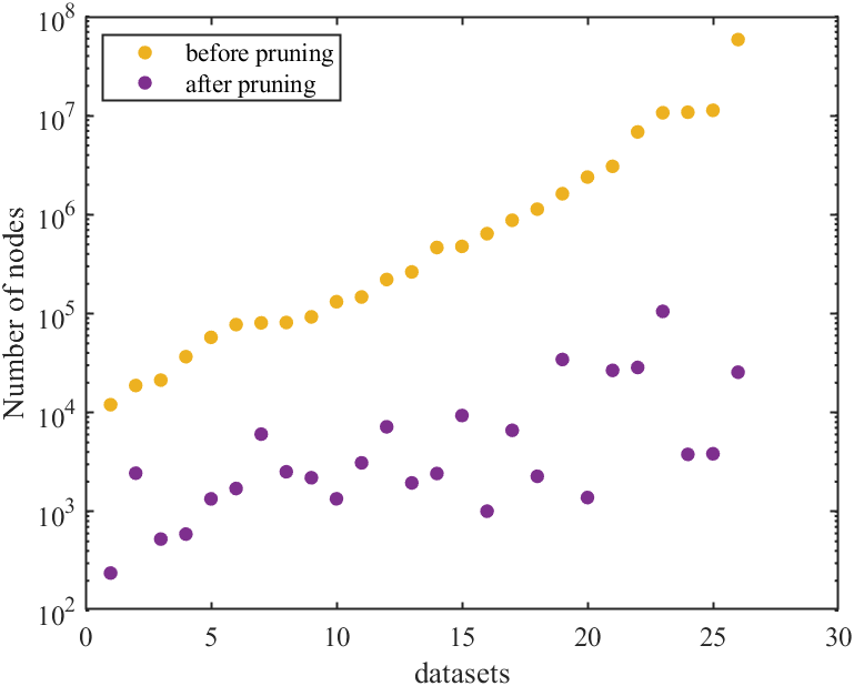
Figure 2: The pruning pre-process reduces the graph size significantly.

IV-A Effectiveness of The Pruning Technique

We choose Max-Flow[6], Greedy in priority tree(PT)[24], Greedy in doubly-linked list(DLL)[10] and Greedy in Balanced Binary Search Tree(BBST)[10] as baseline algorithms. PT, DL, BBST are different data structures used in Greedy, DLL can only be applied on unweighted graphs while BBST and PT can be applied on weighted graphs. We implement Max-Flow, Greedy in PT by ourselves, the code of Greedy in DLL and BBST is from [10] because they optimize it enough well.

Although Core-App[17] can attain $k_{max}$-core efficiently which is also 1/2-approximation like Greedy, its density is no more than the density attained by Greedy because Greedy can choose the subgraph with the maximum density and $k_{max}$-core is attained at Greedy’s some time according to Lemma 2. Therefore, among approximation algorithms, we only select Greedy in different data structures because they can achieve equivalent results.

Figure 2 compares the size of graphs before and after the pruning pre-process. We can see that applying the pruning leads to about two orders of magnitude of reduction for the size of all networks. The effect of pruning is more obvious on larger graphs.

TABLE IV: Comparison between Lowd and baselines.

		Running time					The number of iteration rounds
Dataset	$|\mathcal{H}^{\prime}|$	LOWD	Greedy++	FW	FISTA	FW-M	LOWD	Greedy++	FW	FISTA	FW-M
ca-HepPh	239	0.0019	0.0013	0.0018	0.0122	0.0014	1	1	1	1	1
comm-EmailEnron	592	0.0115	0.0187	0.0645	0.2437	0.0163	13	10	78	56	19
ca-AstroPh	2441	0.1202	0.1759	0.7566	2.2657	0.2125	36	28	345	183	83
PP-Pathways	527	0.0089	0.0029	0.0354	0.1023	0.0241	6	1	24	18	16
soc-sign_slashdot	1709	0.0255	0.0045	0.0807	0.3132	0.0361	10	1	42	27	18
soc-sign_epinion	1345	0.0178	0.0830	0.1309	0.2721	0.0700	4	12	43	15	22
soc-Twitter_ICWSM	2423	0.0944	0.5038	4.9809	1.3091	0.9862	39	120	2820	115	573
rating-StackOverflow	1008	0.0199	0.0666	0.1635	0.4072	0.0286	24	45	272	125	44
ego-twitter	2523	0.0929	0.4272	1.9648	0.7245	0.0813	13	46	478	25	19
soc-Youtube	2269	0.1077	0.8683	1.7423	3.6148	0.3113	29	127	608	181	106
comm-WikiTalk	1384	0.0099	0.0107	0.0094	0.0412	0.0093	1	1	1	1	1
nov_user_msg_time	3779	3.026	5.5366	12.2961	19.9690	2.1637	96	72	436	91	76
cit-Patents_AMINER	28546	2.3379	29.3613	23.5359	44.4324	10.5380	17	65	224	43	100
soc-Twitter_ASU	3834	0.1189	0.2180	0.1034	0.5913	0.1088	1	1	1	1	1
soc-Livejournal	105265	152.9460	13795.667	24839.696	57567.91	1322.3124	437	8436	83549	17099	4615
soc-Orkut	26670	14.9269	111.2410	1440.7987	1661.6384	86.1052	71	150	8242	1063	495
soc-SinaWeibo	25556	36.0107	308.7090	2694.3677	3020.8957	280.3085	262	594	21266	2589	2263
wang-tripadvisor	3103	0.0708	0.8382	1.7039	2.4322	0.6695	121	187	4031	941	1403
rec-YelpUserBusiness	1343	0.0732	1.5679	0.7741	3.7359	0.0987	46	207	784	466	104
bookcrossing	1946	0.0703	1.6941	1.0291	5.9866	0.1824	75	278	1383	1516	250
librec-ciaodvd-review	2195	0.2090	3.6041	14.9112	33.9615	0.2609	49	139	4644	958	80
movielens-10m	6049	0.1322	0.5096	0.1245	1.5077	0.1249	1	1	1	1	1
epinions	6616	1.2117	140.5527	187.0548	268.6413	5.0036	43	788	9081	1473	239
libimseti	7179	1.1102	247.5964	57.4351	384.2001	3.0025	18	594	1142	912	59
rec-movielens	9335	8.8373	839.4542	83.8077	635.9382	1.7434	52	738	563	480	11
yahoo-song	34352	155.6296	11453.641	4144.8288	46170.844	51.6024	154	1532	4959	4892	61
note: $|\mathcal{H}^{\prime}|$ denotes the size of the subgraph after the pruning, FW means Frank-Wolfe in [8].

We compare the running time of the approximation and exact algorithms on weighted and unweighted graphs in Table III, where the results are the average of 5 trails. We report the density of detected subgraphs by approximation and exact algorithms in the appendix. The density obtained by the same type of algorithm is equivalent (We use $||$ to distinguish different types). It shows that the pruning can save a lot of time for subsequent algorithms, i.e., Greedy in different data structures and Max-Flow; the pruning achieves the best results (as the bold labeled) on both weighted graphs and unweighted graphs.

Columns 2 and 3 are the pruning used on weighted and unweighted graphs respectively (Of course an unweighted graph can be seen as a weighted graph with $w_{e}=1$ for any edge $e$). They prune the graph and lock the densest subgraph into a much smaller range.

Columns 4-6 show the results of approximation algorithms for all networks, we can find that PT is much faster than BBST. Although BBST has the same average time complexity as PT, i.e., $O(M\log N)$, it actually runs much slower than PT, especially on large datasets, which is attributed to the higher probability of a worse situation in BBST since deleting the node with the lowest weight iteratively in Greedy is not a balanced operation in BBST. Therefore, we just combine the pruning technique with PT, and it can detect the same subgraph faster, which achieves about $3.563\times$ on average by utilizing the pruning technique than using PT alone.

Although the time complexity of the pruning on weighted graphs is $O(M+TN)$ and we are not sure about the iteration count $T$, in our experiments, the number of deleted nodes approximately obeys the exponential law (in the appendix we plot 6 datasets to illustrate the exponential law). Therefore, $T$ is $O(\log N)$ according to experimental performance so the pruning is also efficient on weighted graphs, which can be confirmed with the results of columns 5 and 6, i.e., w_Pruning+PT runs faster than using PT alone.

Columns 7-8 are the results of the exact algorithms. It shows that the pruning accelerates Max-Flow by $28.215\times$ on average (ignoring the time-out datasets, although it performs better on large datasets), which can be attributed to two reasons: First, a higher density lower bound $\delta$ for the subsequent binary search. Second, a smaller graph needs to be explored next. These factors greatly reduce the number of binary-search iterations and the execution time of the max flow algorithm.

Columns 9-10 are the results of approximation algorithms for unweighted graphs. Greedy in doubly-linked list achieves $2.312\times$ speedup on average by utilizing the pruning. Although the speed of uw_Pruning is not faster than that of w_Pruning evidently, it has an accurate time complexity, i.e., $O(M+N)$. By utilizing the pruning technique, we acelerate DLL about $2.312\times$ on average.

IV-B Effectiveness of Lowd When Solving DSP

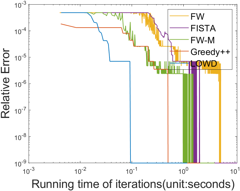
(a) soc-Twitter_ICWSM

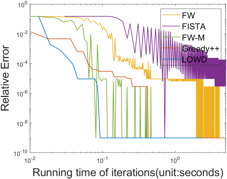
(b) ego-twitter

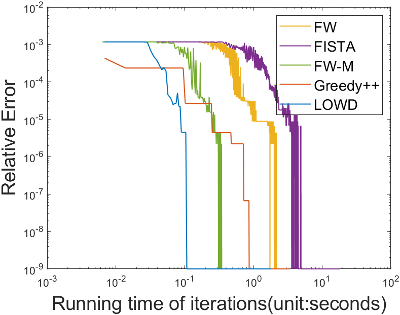
(c) soc-Youtube

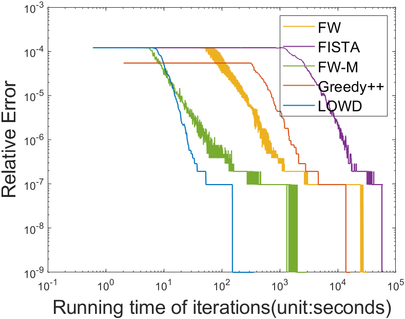
(d) soc-Livejournal

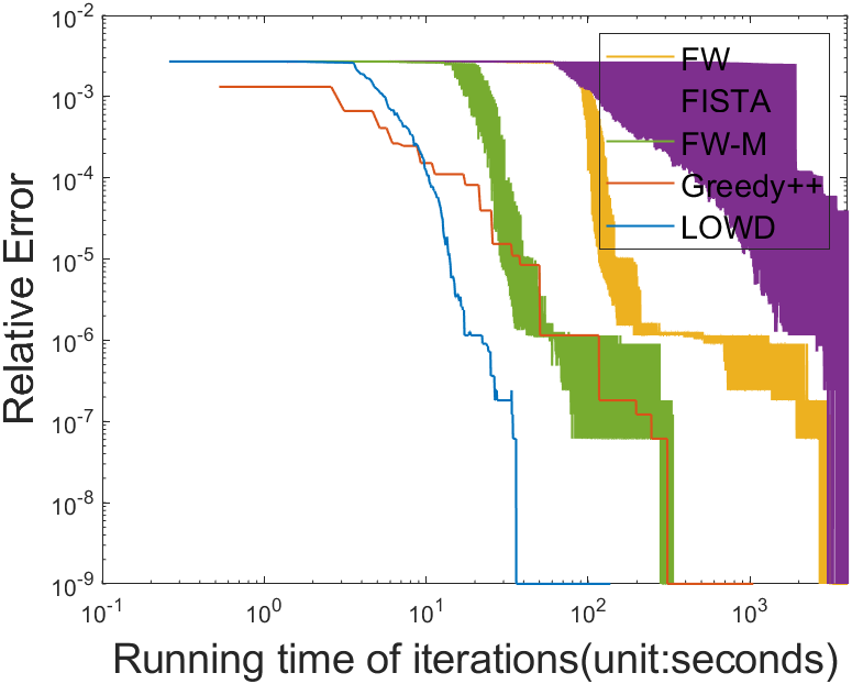
(e) soc-SinaWeibo

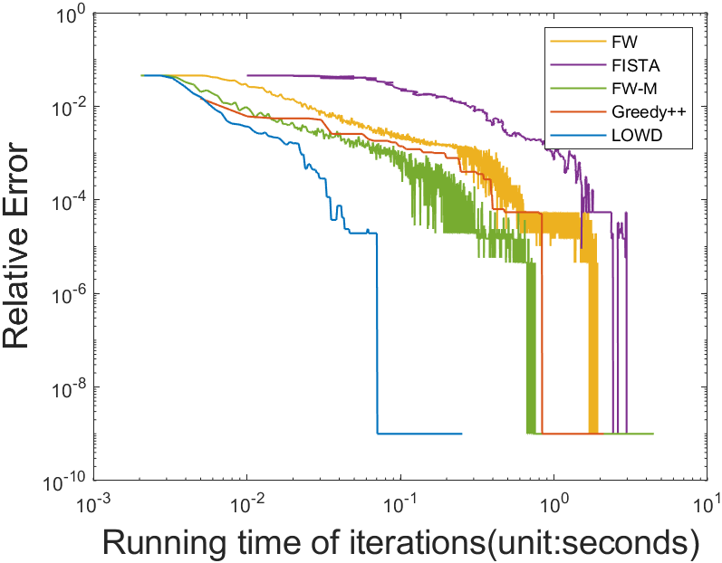
(f) wang-tripadvisor

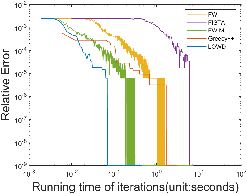
(g) bookcrossing

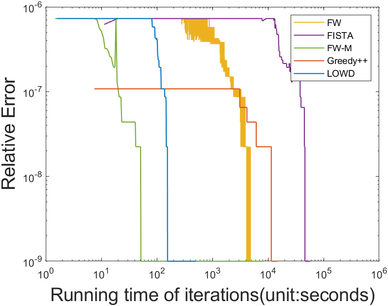
(h) yahoo-song

Figure 3: Comparison on detecting the densest subgraph.

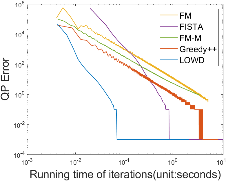
(a) soc-Twitter_ICWSM

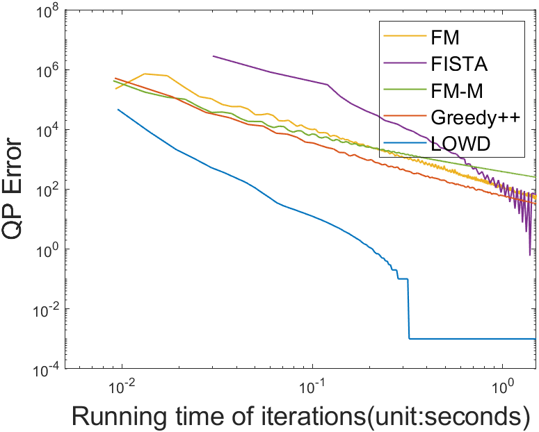
(b) ego-twitter

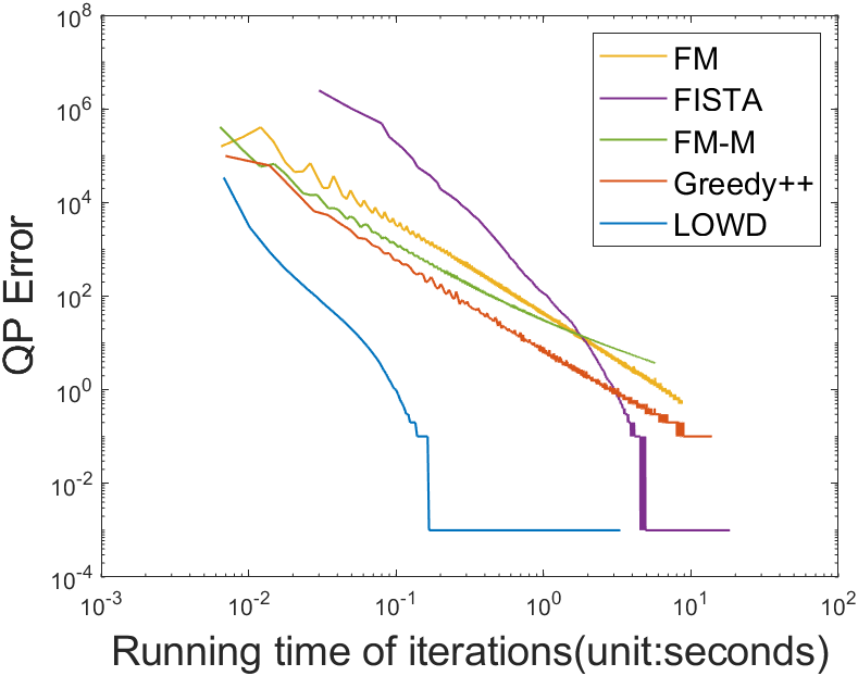
(c) soc-Youtube

(d) soc-Livejournal

(e) soc-SinaWeibo

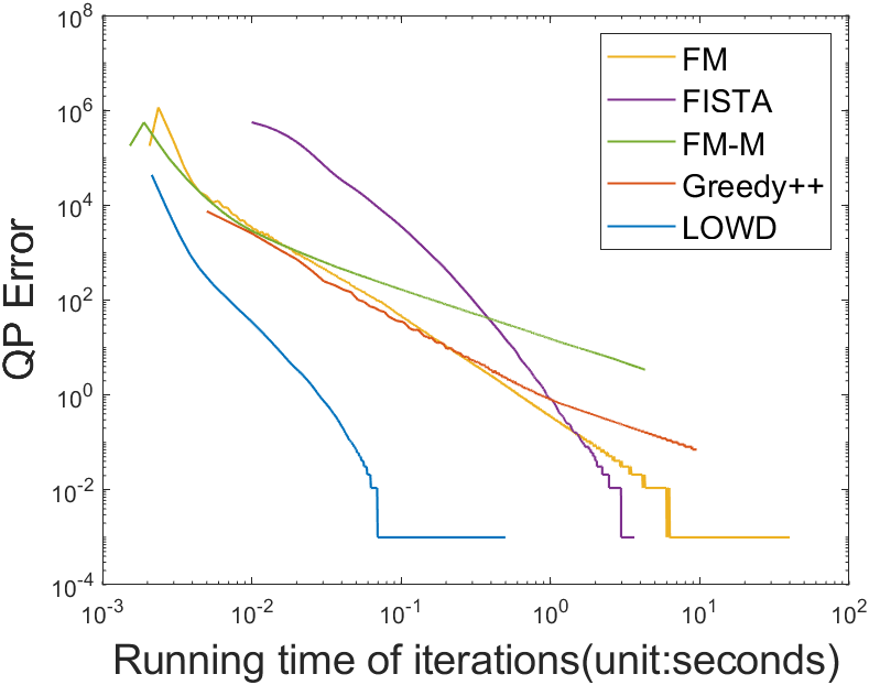
(f) wang-tripadvisor

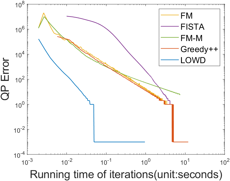
(g) bookcrossing

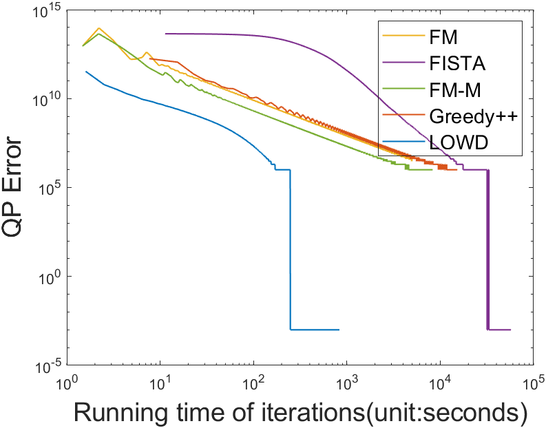
(h) yahoo-song

Figure 4: Comparison on detecting the locally-dense decomposition.

To fully demonstrate the efficiency of Lowd, we compare it with the state-of-the-art iterative algorithms including Frank-Wolfe(FW) in [8], Greedy++ in [10] and FISTA in [12], we also compare it with ”Frank-Wolfe with a modified learning rate”(FW-M), the original learning-rate for Frank-Wolfe is $\frac{2}{(t+2)}$(t is the iteration number) while learning-rate in FW-M is $\frac{1}{(t+1)}$ inspired by [12]. FISTA and Greedy++ are implemented based on their own original codes, while Frank-Wolfe and its variant(FW-M) are implemented by ourselves. In this subsection, we want to figure out how well these iterative algorithms perform on detecting the densest subgraph and fully demonstrate the effectiveness of Lowd. We devise our experiments as below:

• Comparison on detecting the densest subgraph. We execute it to figure out whether Lowd can perform better than other iterative algorithms on detecting the densest subgraph.

• The relative error on the density as iterations count increases. We supplement it to exhibit the convergence speed of Lowd and other iterative algorithms on 8 randomly selected datasets.

All these experiments are executed with the pruning technique to pre-process these datasets. Corresponding experiments without the pruning are also executed whose results are listed in the appendix.

We initialize Lowd, Frank-Wolfe, FISTA and FW-M by distributing the weight of each edge equally to its associated nodes like lines 1-4 in Algorithm 1, which makes the node weight positively correlated with its degree, our intuitive consideration is that nodes with higher degrees should not be deleted first while it is unclear which node each edge should be distributed to. This sort method is also used in [8].

In Table IV, we compared Lowd and other baselines on the subgraphs after pruning in Algorithm 2 on unweighted and weighted graphs. The optimal result is bolded and underlined, while the suboptimal result is only underlined. It shows that Lowd detects the densest subgraphs much faster than other iterative algorithms from the overall experimental performance, most of its results are optimal or suboptimal. Besides, Greedy++ is easier to detect the densest subgraph in only one iteration, which partly shows the effectiveness of Greedy. FW-M needs fewer iteration rounds than using its original learning-rate and FISTA needs more time to detect DSP in this sorting method(sorting node load and deleting the node with the lowest load one by one). However, it is worth mentioned that DSP is a subproblem of LDD. Actually FISTA has a better convergence speed than other baselines when solving LDD and FW-M doesn’t converge faster than FW according to Figure 4. And [12] devised a method called ”fractional peeling” to detect the densest subgraph faster than the sorting method in our experiments. Related theory and experiments can be seen in [12]. To be accurate, FW-M suits the sorting method better while FW, FISTA don’t suit it very much (which can be improved by ”fractional peeling”). And our method Lowd performs best both in DSP and LDD. The following paragraph will provide more detailed information.

Next, we randomly choose 8 datasets to exhibit the relative error of these algorithms as iterations count increases. The definition of relative error is: $(\rho^{*}-\rho(\mathcal{S}))/\rho^{*}$. We use logarithmic coordinates to exhibit it more explicitly. We add a small amount eps=1e-9 to the relative error because when we detect the graph with density $\rho(\mathcal{S})=\rho^{*}$, its relative error is 0 and doesn’t appear on logarithmic coordinates. Lowd has the optimal convergence speed on 7 datasets and the suboptimal convergence speed on 1 dataset, which is slower than FW-M. Lowd’s relative error seldom vibrates because it monotonically decreases the optimization of LP 3 and QP 4 based on its local optimality. Greedy doesn’t vibrate because it stores the best result of all iterations while the relative errors of Frank-Wolfe, FISTA and FW-M vibrate apparently because they are based on classical methods towards convex optimization like gradient descent and its variants. They don’t ensure monotonic decline, which we will observe again in experiments about LDD.

IV-C Effectiveness of Lowd When Solving LDD

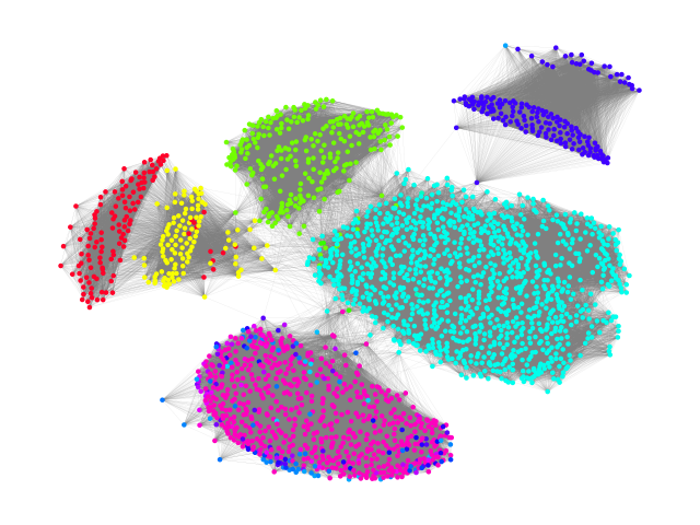
Figure 5: LDD in ego-twitter (500 iterations of Lowd)

We also conduct experiments about the convergence speed to the locally-dense decomposition in Figure 4. The definition of QP error on the y-axis is: $\sum_{v\in\mathcal{V}}{{\ell_{v}}^{2}}-\sum_{v\in\mathcal{V}}{{\ell_{v}^{*}}^{2}}$, where $\sum_{v\in\mathcal{V}}{{\ell_{v}}^{2}}$ is attained by these iterative algorithms and $\sum_{v\in\mathcal{V}}{{\ell_{v}^{*}}^{2}}$ is the optimal value of QP (4). We use the minimum $\sum_{v\in\mathcal{V}}{{\ell_{v}}^{2}}$ attained by these algorithms to represent the optimal value and add a small amount eps=1e-3 to QP error similarly.

From Figure 4, we can see that Lowd optimize $\sum_{v\in\mathcal{V}}{{\ell_{v}}^{2}}$ much faster than any other iterative algorithms because the x-axis is logarithmic coordinate. We conclude this to the local optimality of Lowd in QP (4). FISTA performs better on LDD than FW-M, Frank-Wolfe and Greedy++, which is consistent with the conclusion in [12]. In Figure 4 all baselines will vibrate to some degree, while our method Lowd can optimize QP (4) monotonically.

To observe the locally-dense decomposition, we run Lowd 500 iterations on ego-twitter after pruning to achieve Figure 5 as an example. We use colormap $gist\_rainbow$ in $matplotlib$ to dye nodes according to their loads, therefore, nodes with the same loads should have the same color. In Figure 5 red means the minimum node load and violet means the maximum node load. And the nodes with maximum loads represent $B_{1}$ and the nodes with the second largest loads represent $B_{1}\setminus B_{2}$. We can really observe the hierarchical phenomenon on node loads in locally-dense decomposition. Besides, we checked some edges with $e=(u,v)$ and $u$,$v$ have different node loads, and these edge weights are all distributed in one-way to endpoints with lower loads. Another interesting discovery is that the node position is based on the Kamada-Kawai path-length in $matplotlib$, we can see nodes with similar loads are close to each other, which also implies that Kamada-Kawai path-length has connections with locally-dense decomposition.

By observing the locally-dense decomposition, it not only helps to detect different variants of the densest subgraph like DkS in Corollary 1 and locally densest subgraph in [15], but also helps us to understand the whole graph about the theme of ”edge-density”. Given that we get the densest subgraph by distributing edge weights, we can understand the reason why some nodes with high degrees are not in the densest subgraph is that they have to distribute some edge weights to their neighbors with low loads. The influence is transmitted along edges, so the loads of two nodes can be influenced by each other as long as they are in the same connected branch. The previous work [25] has found this phenomenon, they generalized the Greedy algorithm of [7] with a parameter $p$ (the Greedy algorithm is equal to the generalized form with $p=1$) and set $p=1.05$ to spread the influence of node neighbors slightly, which helps to detect denser subgraphs than Greedy.

V Related work

The most recent surveys [26, 27] present a systematic, thorough overview and summarization of the densest subgraph problem, and the tutorials [28, 29] also give a comprehensive survey of the discovery of the densest subgraphs on large graphs and discuss the challenges and various applications.

For the graph with non-negative edge weights, the densest subgraph can be identified in polynomial time by solving a maximum flow problem [6, 30, 13]; Charikar [7] introduces a linear programming formulation of the problem and shows that the greedy algorithm proposed by Asashiro et al. [31] produces a $\frac{1}{2}$-approximation of the optimal density in linear time. [8] devises an efficient algorithm via convex programming, which can compute the exact locally-dense decomposition in real graphs with billions of edges, and proposes an $(1+\epsilon)$-approximation solution based on the Frank-Wolfe algorithm. Boob et al. [10] developed a simple iterative peeling algorithm Greedy++ to improve the quality of the subgraph over Charikar’s greedy algorithm by drawing insights from the iterative approaches (multiplicative weights update) of convex optimization; the history of peeling information of nodes will help to escape the local solution to some extent. [9] provided an algorithm for maintaining an $(1-\epsilon)$-approximate (arbitrarily close to 1) densest subgraph within $O(\mathrm{poly}\log n)$ time over dynamic directed graphs, and extended to solve the problem on vertex-weighted static graphs. Feng et al. [32] proposed a generalized framework for addressing DSP and related problems [24, 33, 34, 35] and introduced SpecGreedy, an algorithm that leverages the graph spectral properties to a greedy peeling strategy to solve the generalized problem and speed up the detection. Chekuri et al. [11] exploited the supermodular maximization and proposed more efficient $(1-\epsilon)$-approximation algorithms in deterministic $\tilde{O}(m/\epsilon)$ time via approximate flow techniques for DSP, and gives evidence of the convergence and theoretical truthfulness of Greedy++, that is, it can converge to a $(1-\epsilon)$-approximation in $O(1/\epsilon^{2})$ iterations; it also developed an $\frac{1}{2}$-approximation peeling algorithm for the densest-at-least-k subgraph. [36] modified Greedy++ to have a quantitative certificate of the solution quality provided by the algorithm at each iteration. [12] proposed another iterative method using Proximal Gradient Method, which achieves $(1-\epsilon)$-approximation in $O(1/\epsilon)$, they also proposed a technique called Fractional Peeling to make use of the information in edge distribution. For directed graphs, the LP-based approach proposed by Charikar [7] requires the computation of $n^{2}$ linear programs, and the $\frac{1}{2}$-approximation runs $O(n^{3}+mn^{2})$ time, [37] provided more efficient implementations for these algorithms for undirected and directed graphs.

There is another research line that discovers the densest subgraph building upon some microstructures (motifs) in a graph, including the triangles [38, 39], cliques [40, 41, 17], $k$-core [42], $k$-club / $k$-plex, etc., and proposed corresponding different variants for the density measures. [43, 38] extended the DSP to the $k$-clique, and the $(p,q)$-biclique densest subgraph problems, which can be used to find large near-cliques. Tatti and Gionis [14, 16] introduced the locally-dense graph decomposition method, which imposes certain insightful constraints on the $k$-core decomposition. [17] proposed exact and approximate solutions by improving the flow-based exact algorithm by locating the densest subgraph in a specific $k$-core, which can be generalized by considering an arbitrary pattern graph and aiming to maximize the average number of occurrences of the pattern in the resulting subgraph. [44] proposed $[x,y]$-core-based algorithms (both exact and approximation) with the divide-and-conquer strategy to find the densest subgraph for directed graphs.

When restrictions on the size of nodeset are imposed, the DSP also becomes NP-hard [45], which is called the densest k-subgraph (DkS). Its two variants called densest at-least-k subgraph (DalkS) and densest at-most-k subgraph (DamkS) are also NP-hard according to [13, 45].

The dense subgraphs are used to detect communities [46, 47, 2] and anomalies [48, 49, 24]. As one of the key characteristics, density, as well as other similar metrics like modularity [50], associativity, and local density [51], are used as (part of) optimization objectives to detect community structures.

VI Conclusion and Future Outlook

In this paper, we propose Lowd to detect the densest subgraph and prove it can converge to locally-dense decomposition. Lowd redistributes edge weight in a locally optimal operation according to the linear programming of the DSP and quadratic programming of locally-dense decomposition. Besides, we develop a pruning technology using modified Counting Sort and prove that it is a subprocess of Greedy. We did a lot of experiments to exhibit its pruning efficiency on 26 real-world datasets and compare it with other algorithms about Greedy and Max-Flow. We also use it to prune the graph to speed up the iterative algorithms. In our experiments, Lowd can converge to the optimal values both in the linear programming of the DSP and quadratic programming of locally-dense decomposition faster than other state-of-the-arts iterative algorithms, including Frank-Wolfe in [8], Greedy++ in [10] and FISTA in [12] and FW-M.

Through our study, there are far more interesting topics in DSP and LDD that we can study in future work. We list them as follows:

1. What is the relationship between the size of the graph after pruning and the size of the whole graph (it’s possibly related to properties of Kronecker graphs in [52], which concerns how graphs evolve)?

2. In our experiments, Kamada-Kawai path-length has a close relationship with LDD because we use Kamada-Kawai path-length to decide the position of nodes. How can we theoretically analyze the relationship between these two things?

3. Can we discover the relation between iteration count $T$ and the approximate ratio?

These problems also show that there is a close relationship among DSP, locally-dense decomposition and other theories in the graph field like DkS and locally densest subgraph in [15]. Understanding the relationship among them can help us mine dense subgraphs in more efficient and meaningful ways, and we can use dense subgraphs to discover more characteristics in the graph.

VII Acknowledgments

We would like to express our sincere gratitude to Mr. Harb Elfarouk[12] for his invaluable contributions to this research. Mr. Elfarouk generously provided us with his algorithm and its codes, which formed the foundation of our work. His willingness to answer our questions and share his expertise played a crucial role in this study.

VIII Full version

Proof of Corollary 1.

For DkS, we set $|\mathcal{S}|=k$, it has an upper bound as follows:

$$\rho(\mathcal{S}) =\frac{\sum_{e\in\mathcal{E}(\mathcal{S})}w_{e}}{|\mathcal{S}|}=\frac{\sum_{e=(u,v),\,u,v\in\mathcal{S}}f_{e}(u)+f_{e}(v)}{|\mathcal{S}|}$$

$$\leq\frac{\sum_{e=(u,v),\,u,v\in\mathcal{S}}{(f_{e}(u)+f_{e}(v))}+\sum_{e=(u,v),\,u\in\mathcal{S},v\not\in\mathcal{S}}{f_{e}(u)}}{|\mathcal{S}|}$$

$$=\frac{\sum_{u\in\mathcal{S}}{\sum_{e\ni u}{f_{e}(u)}}}{|\mathcal{S}|}=\frac{\sum_{u\in\mathcal{S}}{l_{u}}}{|\mathcal{S}|}$$

$$=\frac{\sum_{i=0}^{j-1}{\lambda_{i}*|B_{i}|}+(k-|B_{j-1}|)*\lambda_{j}}{k}$$

Therefore, result 2 holds up. As for result 1, if $k=|B_{j}|$, according to property 3 the equivalency condition in line 2 holds up because $f_{e}(u)=0$ if $u\in\mathcal{S}$ and $v\not\in\mathcal{S}$, then result 1 holds up. These results also hold up for DalkS because if $|S|>k$, it will add more nodes into $\mathcal{S}$ with lower upper bounds on their loads. ∎

Before proofs of Lemma 2, we introduce the definition of $k$-core from [53]: $k$-core is the maximal subgraph $G_{k}$ in graph G, the degree of where any vertex $v$ in $G_{k}$ is satisfied with $\mathrm{d}_{G_{k}}(v)\geq k$.

proof of Lemma 2.

The Greedy algorithm just moves any node whose degree is the lowest in the remaining graph $\mathcal{H}$. Let us remark $A(k)$ as the nodeset of k-core for specific k. We claim that when deleting a node $u\in A(k)$, there mustn’t be any node $v\not\in A(k)$ in the remaining graph $\mathcal{H}$. We prove it by way of contradiction, w.l.o.g, we set $u$ as the first node to be deleted in $A(k)$ in Greedy, therefore $u$ has the lowest degree in $\mathcal{H}$ and $\mathrm{d}_{\mathcal{H}}(v)\geq\mathrm{d}_{\mathcal{H}}(u)\geq\mathrm{d}_{A(k)}(u)\geq k$ for any node $v$ in $\mathcal{H}$, which produces a k-core subgraph with a larger size, and it leads to a contradiction. ∎

Proof of Theorem 5.

We set $\mathcal{H}_{k}(k>0)$ is the remaining graph after k iterations in Algorithm 2 and $\mathcal{H}_{0}$ is the initial whole graph, $\mathcal{H}_{k+1}^{{}^{\prime}}$ is the nodeset to be deleted in k+1 iteration. Therefore, $\mathcal{H}_{k+1}=\mathcal{H}_{k}\setminus\mathcal{H}_{k+1}^{{}^{\prime}}$,

$$\rho(\mathcal{H}_{k+1}) =\rho(\mathcal{H}_{k}\setminus\mathcal{H}_{k+1}^{{}^{\prime}})$$

$$=\frac{\mathcal{W}(\mathcal{E}(\mathcal{H}_{k}))-\mathcal{W}(\mathcal{E}(\mathcal{H}_{k+1}^{{}^{\prime}}))}{|\mathcal{H}_{k}|-|\mathcal{H}_{k+1}^{{}^{\prime}}|}$$

$$\geq\frac{\rho(\mathcal{H}_{k})\cdot|\mathcal{H}_{k}|-\sum_{v\in\mathcal{H}_{k+1}^{{}^{\prime}}}{\mathrm{d}_{\mathcal{H}_{k}}(v)}}{|\mathcal{H}_{k}|-|\mathcal{H}_{k+1}^{{}^{\prime}}|}$$

$$>\frac{\rho(\mathcal{H}_{k})\cdot|\mathcal{H}_{k}|-\sum_{v\in\mathcal{H}_{k+1}^{{}^{\prime}}}{\rho(\mathcal{H}_{k})}}{|\mathcal{H}_{k}|-|\mathcal{H}_{k+1}^{{}^{\prime}}|}$$

$$=\frac{\rho(\mathcal{H}_{k})\cdot|\mathcal{H}_{k}|-\rho(\mathcal{H}_{k})\cdot|\mathcal{H}_{k+1}^{{}^{\prime}}|}{|\mathcal{H}_{k}|-|\mathcal{H}_{k+1}^{{}^{\prime}}|}$$

$$=\rho(\mathcal{H}_{k})$$

That means the density of graph $\mathcal{H}$ monotonically increases in iterations, then any deleted node has a lower degree (when it is being deleted) than the final density, i.e., $\delta$. Therefore, the remaining graph $\mathcal{H}$ is a $\delta$-core and it is the graph of some time of the greedy search according to Lemma 2.

We claim that the process before getting the $\delta$-core is a monotonic increasing phase of density in Greedy. We can confirm two facts:

1. During Greedy, if there is a node $u\in\mathcal{H}_{1}^{{}^{\prime}}$ existing in the remaining graph, the deletion in Greedy will increase the density of the remaining graph. That’s because if Greedy deletes a node $v\not\in\mathcal{H}_{1}^{{}^{\prime}}$, then $\mathrm{d}_{\mathcal{H}}(v)\leq\mathrm{d}_{\mathcal{H}}(u)<\rho(\mathcal{G})\leq\rho(\mathcal{H})$. $\rho(\mathcal{H})$ will increase and $\rho(\mathcal{G})\leq\rho(\mathcal{H})$ still holds up. If Greedy deletes the node $u$, now that $\mathrm{d}_{\mathcal{H}}(u)\leq\rho(\mathcal{H})$, then $\rho(\mathcal{H})$ will also increase and $\rho(\mathcal{G})\leq\rho(\mathcal{H})$ holds up.

2. During Greedy, if there is a node $u\in\mathcal{H}_{k+1}^{{}^{\prime}}$ existing in the remaining graph $\mathcal{H}>\mathcal{H}_{k}$, and there isn’t any node belonging to $\mathcal{H}_{k}^{{}^{\prime}}$. Then: $\rho(\mathcal{H})\geq\rho(\mathcal{H}_{k})$ because we delete more nodes with lower degrees. Therefore, when we deletes a node $v\not\in\mathcal{H}_{k+1}^{{}^{\prime}}$, then $\mathrm{d}_{\mathcal{H}}(v)\leq\mathrm{d}_{\mathcal{H}}(u)<\rho(\mathcal{G})\leq\rho(\mathcal{H}_{k})\leq\rho(\mathcal{H})$, then $\rho(\mathcal{H})$ will increase and $\rho(\mathcal{G})\leq\rho(\mathcal{H})$ holds up. If Greedy deletes the node $u$, now that $\mathrm{d}_{\mathcal{H}}(v)\leq\rho(\mathcal{H})$, $\rho(\mathcal{H})$ will also increase and $\rho(\mathcal{G})\leq\rho(\mathcal{H})$ holds up.

Therefore, the density monotonically increases in Greedy before getting $\delta$-core. ∎

TABLE V: Dataset source and density of algorithms

Dataset	Source	Type	Pruning	w_app	exact	DLL	uw_Pruning+DLL
ca-HepPh	Stanford’s SNAP database	scholar collaboration network	119	119	119	119	119
comm-EmailEnron	Stanford’s SNAP database	communication	37.316	37.344	37.344	37.337	37.337
ca-AstroPh	Stanford’s SNAP database	scholar collaboration network	28.481	29.616	32.11	29.552	29.552
PP-Pathways	Stanford’s SNAP database	protein interaction network	74.159	77.995	77.995	77.995	77.995
soc-Twitter_ICWSM	konect	social network	25.678	25.683	25.69	25.686	25.685
soc-sign_slashdot	Stanford’s SNAP database	social network	39.376	42.132	42.132	42.132	42.132
rating-StackOverflow	konect	social network	20.209	20.209	20.21	20.209	20.209
soc-sign_epinion	Stanford’s SNAP database	social network	80.168	85.599	85.637	85.589	85.589
ego-twitter	Stanford’s SNAP database	social network	59.281	68.414	69.622	68.414	68.414
soc-Youtube	Stanford’s SNAP database	social network	45.545	45.58	45.599	45.576	45.577
comm-WikiTalk	Stanford’s SNAP database	communication	114.139	114.139	114.139	114.139	114.139
nov_user_msg_time	We own it privately.	social network	278.815	278.815	278.815	278.815	278.815
cit-Patents	AMiner scholar datasets	scholar collaboration network	132.776	135.706	137.261	135.706	135.706
soc-Twitter_ASU	ASU	social network	593.847	593.847	593.847	593.847	593.847
soc-Livejournal	Livejournal	social network	104.596	104.601	104.609	104.603	104.603
soc-Orkut	Stanford’s SNAP database	social network	227.861	227.872	227.874	227.872	227.872
soc-SinaWeibo	Network Repository	social network	164.967	165.193	165.415	165.196	165.191
wang-tripadvisor	konect	rating network	13.442	13.873	14.082	–	–
rec-YelpUserBusiness	Network Repository	rating network	87.825	87.912	87.921	–	–
bookcrossing	konect	rating network	92.148	92.322	92.374	–	–
librec-ciaodvd-review	konect	rating network	233.553	233.59	233.597	–	–
movielens-10m	konect	rating network	1351.35	1351.35	1351.35	–	–
epinions	konect	rating network	595.302	595.314	595.316	–	–
libimseti	konect	social network	1645.71	1645.73	1645.73	–	–
rec-movielens	Network Repository	rating network	1801.16	1801.16	1801.16	–	–
yahoo-song	konect	rating network	46725.2	46725.2	46725.2	–	–
note: : Pruning (w_Pruning,uw_Pruning). w_app: approximation algorihtms on weighted graph(Priority Tree,Pruning+Priority Tree,BBST). exact: exact algorithms(maxflow,w_Pruning+maxflow). DLL:Doubly-linked list.

TABLE VI: Comparison between LOWD and baselines without the pruning.

	Running time					The number of iteration rounds
Dataset	LOWD	Greedy++	FW	FISTA	FW_M	LOWD	Greedy++	FW	FISTA	FW_M
ca-HepPh	0.0168	0.0159	0.0208	0.1109	0.0161	1	1	2	3	1
comm-EmailEnron	0.1516	0.0714	0.5551	27.5346	0.3012	19	2	88	567	46
ca-AstroPh	0.3158	0.8396	2.312	24.2470	0.6593	36	33	343	375	92
PP-Pathways	0.1174	0.0333	0.3214	12.6981	1.7086	8	1	18	131	167
soc-sign_slashdot	0.2275	0.0704	0.7881	11.6623	1.1051	11	1	44	81	64
soc-sign_epinion	0.3213	1.4706	1.1853	11.1319	0.9581	9	12	40	46	33
soc-Twitter_ICWSM	1.8343	30.6654	96.3405	1207.2601	6.1467	49	114	2816	4901	175
rating-StackOverflow	2.1887	1.0537	10.0728	567.1578	18.7819	32	2	178	1125	341
ego-twitter	1.6001	2.9768	22.0971	2567.2520	1.7266	34	21	550	8115	41
soc-Youtube	6.5253	133.3086	82.3855	1001.4894	22.0866	46	129	612	929	161
comm-WikiTalk	4.6758	1.984	118.307	1933.6041	414.9261	15	1	407	1151	1386
nov_user_msg_time	341.1144	4464.4998	2581.9086	9826.2465	718.8805	97	174	624	454	177
cit-Patents_AMINER	291.4452	846.3628	837.8446	27554.332	1523.2698	104	56	259	1913	471
soc-Twitter_ASU	120.8906	19.2912	511.3170	12174.952	2047.9598	40	1	156	1244	603
soc-Livejournal	–	–	–	–	–	–	–	–	–	–
soc-Orkut	–	–	–	–	–	–	–	–	–	–
soc-SinaWeibo_NETREP	–	–	–	–	–	–	–	–	–	–
wang-tripadvisor	0.6686	23.6761	30.209	198.1408	15.6705	93	187	3894	4512	2007
rec-YelpUserBusiness	0.4621	24.5879	5.1698	62.8514	2.1192	54	228	626	886	239
bookcrossing	1.5177	92.9406	27.4916	910.8345	8.877	78	259	1398	5510	448
librec-ciaodvd-review	4.2248	75.7599	231.5822	1882.2756	38.6405	79	143	4635	4339	773
movielens-10m	49.2341	2.7029	129.6344	5329.5159	60.719	159	1	450	1611	211
epinions	30.4071	3957.2229	4302.242	$>$37786.731	743.6429	64	688	8893	$>$10000	1582
libimseti	25.7101	5276.5399	751.3750	24832.745	146.2627	39	710	1196	4632	234
rec-movielens	50.4427	6928.9143	306.0513	24923.281	148.2539	54	733	355	3195	172
yahoo-song	–	–	–	–	–	–	–	–	–	–
note: We ignore some datasets which are very large.”$>$10000” and ”$>$37786.731” means we run 10000 iterations(running time: 37786.731s) and can’t still detect the densest subgraph.

(a) soc-Twitter_ICWSM

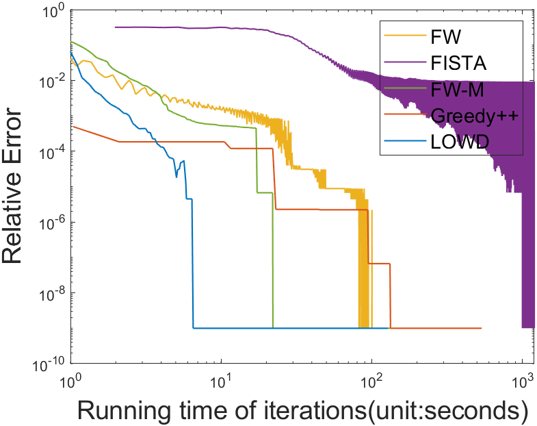
(b) soc-Youtube

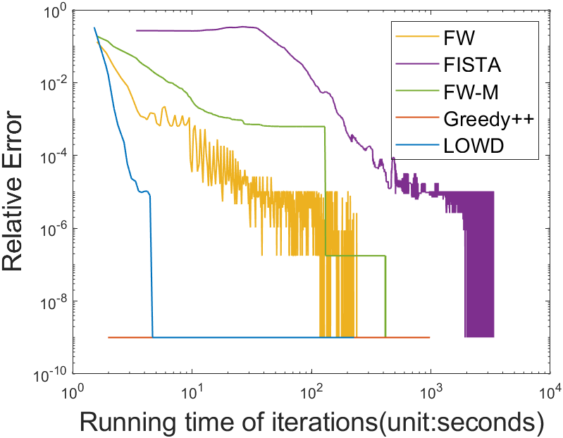
(c) comm-WikiTalk

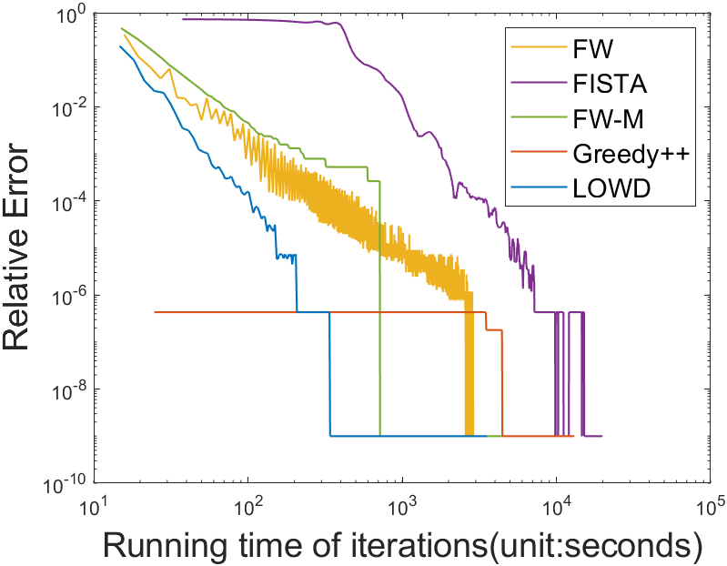
(d) nov_user_msg_time

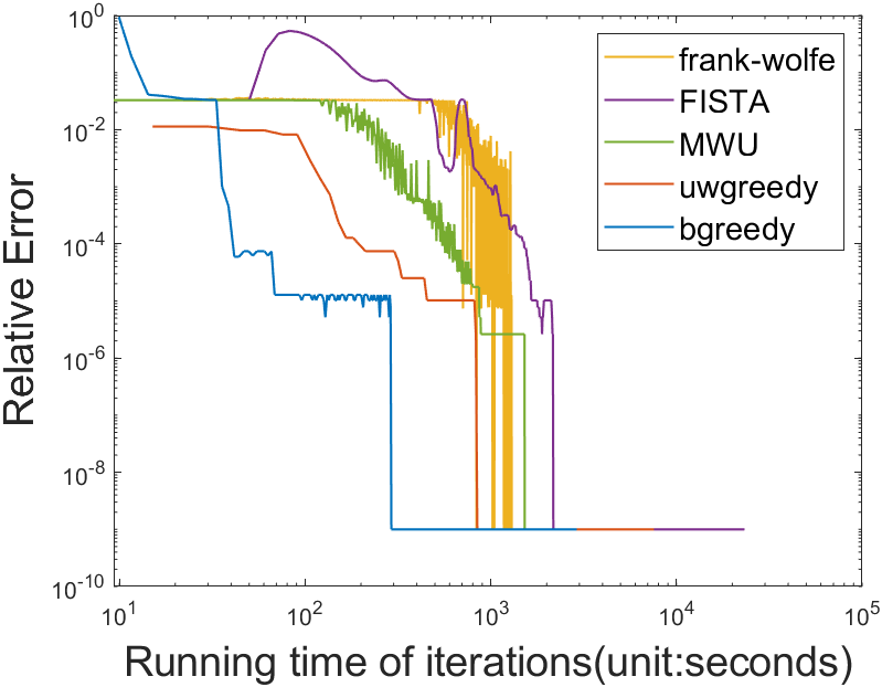
(e) cit-Patents_AMINER

(f) rec-YelpUserBusiness

(g) librec-ciaodvd-review

(h) movielens-10m

Figure 6: densest

Figure 7: Exponential decrease in the number of deleted nodes.

Input: Undirected graph $\mathcal{G}$; density metric $\rho(\cdot)$

Output: $\mathcal{S}^{*}$: the nodeset of the densest subgraph of $\mathcal{G}$.

1 $\mathcal{S},\,\mathcal{S}^{*}\leftarrow\mathcal{V}$

2while $\mathcal{S}\neq\emptyset$ do

3       $\triangleright$ find the vertex $u^{*}$ with the lowest degree in $\mathcal{S}$

4      $u^{*}\leftarrow\operatorname*{arg\,min}_{u\in\mathcal{S}}\mathrm{d}_{\mathcal{S}}(u))$

5      Remove $u^{*}$ and all its adjacent edges from $\mathcal{G}$.

6      $\triangleright$ $\mathcal{S}\backslash\{u\}$: the remaining nodeset without $u$

7      $\mathcal{S}\leftarrow\mathcal{S}\backslash\{u\}$

8      if $\rho(\mathcal{S})>\rho(\mathcal{S}^{*})$ then

9            

10            $\mathcal{S}^{*}\leftarrow\mathcal{S}$

11      

12

return $\mathcal{S}^{*}$.

Algorithm 3 Greedy DSPSolver

References

- [1] H.-W. Shen and X.-Q. Cheng, “Spectral methods for the detection of network community structure: a comparative analysis,” JSTAT, 2010.
- [2] S. W. Wong, C. Pastrello, M. Kotlyar, C. Faloutsos, and I. Jurisica, “Sdregion: Fast spotting of changing communities in biological networks,” in SIGKDD’18, 2018.
- [3] Y. Liu, L. Zhu, P. Szekely, A. Galstyan, and D. Koutra, “Coupled clustering of time-series and networks,” in SDM. SIAM, 2019.
- [4] E. Cohen, E. Halperin, H. Kaplan, and U. Zwick, “Reachability and distance queries via 2-hop labels,” SIAM Journal on Computing, vol. 32, no. 5, pp. 1338–1355, 2003.
- [5] R. Jin, Y. Xiang, N. Ruan, and D. Fuhry, “3-hop: a high-compression indexing scheme for reachability query,” in Proceedings of the 2009 ACM SIGMOD International Conference on Management of data, 2009, pp. 813–826.
- [6] A. V. Goldberg, “Finding a maximum density subgraph,” 1984.
- [7] M. Charikar, “Greedy approximation algorithms for finding dense components in a graph,” in APPROX’00, 2000.
- [8] M. Danisch, T.-H. H. Chan, and M. Sozio, “Large scale density-friendly graph decomposition via convex programming,” in WWW, 2017.
- [9] S. Sawlani and J. Wang, “Near-optimal fully dynamic densest subgraph,” in Proceedings of the 52nd Annual ACM SIGACT Symposium on Theory of Computing, 2020, pp. 181–193.
- [10] D. Boob, Y. Gao, R. Peng, S. Sawlani, C. Tsourakakis, D. Wang, and J. Wang, “Flowless: Extracting densest subgraphs without flow computations,” in Proceedings of The Web Conference 2020, 2020, pp. 573–583.
- [11] C. Chekuri, K. Quanrud, and M. R. Torres, “Densest subgraph: Supermodularity, iterative peeling, and flow,” in Proceedings of the 2022 Annual ACM-SIAM Symposium on Discrete Algorithms (SODA). SIAM, 2022, pp. 1531–1555.
- [12] E. Harb, K. Quanrud, and C. Chekuri, “Faster and scalable algorithms for densest subgraph and decomposition,” Advances in Neural Information Processing Systems, vol. 35, pp. 26 966–26 979, 2022.
- [13] S. Khuller and B. Saha, “On finding dense subgraphs,” in Automata, Languages and Programming: 36th International Colloquium, ICALP 2009, Rhodes, Greece, July 5-12, 2009, Proceedings, Part I 36. Springer, 2009, pp. 597–608.
- [14] N. Tatti and A. Gionis, “Density-friendly graph decomposition,” in WWW, 2015.
- [15] C. Ma, R. Cheng, L. V. Lakshmanan, and X. Han, “Finding locally densest subgraphs: a convex programming approach,” Proceedings of the VLDB Endowment, vol. 15, no. 11, pp. 2719–2732, 2022.
- [16] N. Tatti, “Density-friendly graph decomposition,” ACM Transactions on Knowledge Discovery from Data (TKDD), vol. 13, no. 5, pp. 1–29, 2019.
- [17] Y. Fang, K. Yu, R. Cheng, L. V. Lakshmanan, and X. Lin, “Efficient algorithms for densest subgraph discovery,” arXiv: Databases, 2019.
- [18] J. Bibby, “Axiomatisations of the average and a further generalisation of monotonic sequences,” Glasgow Mathematical Journal, vol. 15, no. 1, pp. 63–65, 1974.
- [19] J. Leskovec and A. Krevl, “SNAP Datasets: Stanford large network dataset collection,” http://snap.stanford.edu/data, Jun. 2014.
- [20] H. Wan, Y. Zhang, J. Zhang, and J. Tang, “Aminer: Search and mining of academic social networks,” Data Intelligence, 2019.
- [21] R. A. Rossi and N. K. Ahmed, “The network data repository with interactive graph analytics and visualization,” in AAAI, 2015. [Online]. Available: http://networkrepository.com
- [22] R. Zafarani and H. Liu, “Social computing data repository at ASU,” 2009. [Online]. Available: http://socialcomputing.asu.edu
- [23] J. Kunegis, “Konect: the koblenz network collection,” in WWW, 2013, pp. 1343–1350.
- [24] B. Hooi, H. A. Song, A. Beutel, N. Shah, K. Shin, and C. Faloutsos, “Fraudar: Bounding graph fraud in the face of camouflage,” in SIGKDD, 2016.
- [25] N. Veldt, A. R. Benson, and J. Kleinberg, “The generalized mean densest subgraph problem,” in Proceedings of the 27th ACM SIGKDD Conference on Knowledge Discovery & Data Mining, 2021, pp. 1604–1614.
- [26] T. Lanciano, A. Miyauchi, A. Fazzone, and F. Bonchi, “A survey on the densest subgraph problem and its variants,” arXiv preprint arXiv:2303.14467, 2023.
- [27] W. Luo, C. Ma, Y. Fang, and L. V. Lakshman, “A survey of densest subgraph discovery on large graphs,” arXiv preprint arXiv:2306.07927, 2023.
- [28] A. Gionis and C. E. Tsourakakis, “Dense subgraph discovery: Kdd 2015 tutorial,” in KDD, 2015.
- [29] Y. Fang, W. Luo, and C. Ma, “Densest subgraph discovery on large graphs: applications, challenges, and techniques,” Proceedings of the VLDB Endowment, vol. 15, no. 12, pp. 3766–3769, 2022.
- [30] G. Gallo, M. D. Grigoriadis, and R. E. Tarjan, “A fast parametric maximum flow algorithm and applications,” SIAM Journal on Computing, vol. 18, no. 1, pp. 30–55, 1989.
- [31] Y. Asahiro, K. Iwama, H. Tamaki, and T. Tokuyama, “Greedily finding a dense subgraph,” Journal of Algorithms, 2000.
- [32] W. Feng, S. Liu, D. Koutra, H. Shen, and X. Cheng, “Specgreedy: unified dense subgraph detection,” in Machine Learning and Knowledge Discovery in Databases: European Conference, ECML PKDD 2020, Ghent, Belgium, September 14–18, 2020, Proceedings, Part I. Springer, 2021, pp. 181–197.
- [33] A. Miyauchi and N. Kakimura, “Finding a dense subgraph with sparse cut,” in CIKM, 2018.
- [34] A. Anagnostopoulos, L. Becchetti, A. Fazzone, C. Menghini, and C. Schwiegelshohn, “Spectral relaxations and fair densest subgraphs,” in CIKM, 2020.
- [35] C. E. Tsourakakis, T. Chen, N. Kakimura, and J. W. Pachocki, “Novel dense subgraph discovery primitives: Risk aversion & exclusion queries,” ECML-PKDD, 2019.
- [36] A. Fazzone, T. Lanciano, R. Denni, C. E. Tsourakakis, and F. Bonchi, “Discovering polarization niches via dense subgraphs with attractors and repulsers,” Proceedings of the VLDB Endowment, vol. 15, no. 13, pp. 3883–3896, 2022.
- [37] S. Khuller and B. Saha, “On finding dense subgraphs,” in Proceedings of the 36th International Colloquium on Automata, Languages and Programming: Part I, ser. ICALP ’09. Springer-Verlag, 2009.
- [38] C. Tsourakakis, “The k-clique densest subgraph problem,” in WWW, 2015.
- [39] R. Samusevich, M. Danisch, and M. Sozio, “Local triangle-densest subgraphs,” in 2016 IEEE/ACM International Conference on Advances in Social Networks Analysis and Mining (ASONAM). IEEE, 2016, pp. 33–40.
- [40] B. Sun, M. Danisch, T. Chan, and M. Sozio, “Kclist++: A simple algorithm for finding k-clique densest subgraphs in large graphs,” Proceedings of the VLDB Endowment (PVLDB), 2020.
- [41] C. Tsourakakis, F. Bonchi, A. Gionis, F. Gullo, and M. Tsiarli, “Denser than the densest subgraph: extracting optimal quasi-cliques with quality guarantees,” in SIGKDD, 2013, pp. 104–112.
- [42] E. Galimberti, F. Bonchi, and F. Gullo, “Core decomposition and densest subgraph in multilayer networks,” in CIKM, 2017.
- [43] M. Mitzenmacher, J. Pachocki, R. Peng, C. Tsourakakis, and S. C. Xu, “Scalable large near-clique detection in large-scale networks via sampling,” in KDD, 2015.
- [44] C. Ma, Y. Fang, R. Cheng, L. V. Lakshmanan, W. Zhang, and X. Lin, “Efficient algorithms for densest subgraph discovery on large directed graphs,” in SIGMOD, 2020.
- [45] R. Andersen and K. Chellapilla, “Finding dense subgraphs with size bounds,” in WAW’09.
- [46] J. Chen and Y. Saad, “Dense subgraph extraction with application to community detection,” IEEE TKDE, 2010.
- [47] A. Costa, “Milp formulations for the modularity density maximization problem,” European Journal of Operational Research, 2015.
- [48] B. A. Prakash, A. Sridharan, M. Seshadri, S. Machiraju, and C. Faloutsos, “Eigenspokes: Surprising patterns and scalable community chipping in large graphs,” in PAKDD, 2010.
- [49] A. Beutel, W. Xu, V. Guruswami, C. Palow, and C. Faloutsos, “Copycatch: stopping group attacks by spotting lockstep behavior in social networks,” in WWW, 2013, pp. 119–130.
- [50] M. E. Newman, “Modularity and community structure in networks,” Proceedings of the national academy of sciences, 2006.
- [51] L. Qin, R.-H. Li, L. Chang, and C. Zhang, “Locally densest subgraph discovery,” in SIGKDD, 2015, pp. 965–974.
- [52] J. Leskovec, D. Chakrabarti, J. Kleinberg, C. Faloutsos, and Z. Ghahramani, “Kronecker graphs: an approach to modeling networks.” Journal of Machine Learning Research, vol. 11, no. 2, 2010.
- [53] S. B. Seidman, “Network structure and minimum degree,” Social networks, vol. 5, no. 3, pp. 269–287, 1983.
- [54] Y. Zhu, S. Liu, W. Feng, X. Cheng,“Fast Searching The Densest Subgraph And Decomposition With Local Optimality,” arXiv preprint arXiv: 2307.15969, 2023.