Gauge-independent transition dividing the confinement phase in the lattice SU(2) gauge-adjoint scalar model.

Abstract

The lattice SU(2) gauge-scalar model with the scalar field in the adjoint representation of the gauge group has two completely separated confinement and Higgs phases according to the preceding studies based on numerical simulations which have been performed in the specific gauge fixing based on the conventional understanding of the Brout-Englert-Higgs mechanism.

In this paper, we re-examine this phase structure in the gauge-independent way based on the numerical simulations performed without any gauge fixing. This is motivated to confirm the recently proposed gauge-independent Brout-Englert-Higgs mechanism for generating the mass of the gauge field without relying on any spontaneous symmetry breaking. For this purpose we investigate correlation functions between gauge-invariant operators obtained by combining the original adjoint scalar field and the new field called the color-direction field which is constructed from the gauge field based on the gauge-covariant decomposition of the gauge field due to Cho-Duan-Ge-Shabanov and Faddeev-Niemi.

Consequently, we reproduce gauge-independently the transition line separating confinement phase and Higgs phase, and show surprisingly the existence of a new transition line that divides completely the confinement phase into two parts. Finally, we discuss the physical meaning of the new transition and implications to confinement mechanism.

I Introduction

In this paper, we investigate the gauge-scalar model to clarify the mechanism of confinement in the Yang-Mills theory in the presence of matter fields and also non-perturbative characterization of the Brout-Englert-Higgs (BEH) mechanism Higgs1 providing the gauge field with the mass, in the gauge-independent way.

For concreteness, we reexamine the lattice $SU(2)$ gauge-scalar model with a radially-fixed scalar field (no Higgs mode) which transforms according to the adjoint representation of the gauge group $SU(2)$ without any gauge fixing. In fact, this model was investigated long ago in Brower82 by taking a specific gauge, say unitary gauge, based on the traditional characterization for the BEH mechanism to identify the Higgs phase. It is a good place to recall the traditional characterization of the BEH mechanism: If the original continuous gauge group is spontaneously broken, the resulting massless Nambu-Goldstone particle is absorbed into the gauge field to provide the gauge field with the mass. In the perturbative treatment, such a spontaneous symmetry breaking is signaled by the non-vanishing vacuum expectation value of the scalar field. However, this is impossible to realize on the lattice unless the gauge fixing condition is imposed, since gauge non-invariant operators have vanishing vacuum expectation value on the lattice without gauge fixing due to the Elitzur theorem Elitzur75 . This traditional characterization of the BEH mechanism prevents us from investigating the Higgs phase in the gauge-invariant way.

This difficulty can be avoided by using the gauge-independent description of the BEH mechanism proposed recently by one of the authors Kondo16 ; Kondo18 , which needs neither the spontaneous breaking of gauge symmetry, nor the non-vanishing vacuum expectation value of the scalar field. Then we can give a gauge-invariant definition of the mass for the gauge field resulting from the BEH mechanism. Therefore, we can study the Higgs phase in the gauge-invariant way on the lattice without gauge fixing based on the lattice construction of gauge-independent description of the BEH mechanism. Consequently, we can perform numerical simulations without any gauge-fixing and compare our results with those of the preceding result Brower82 obtained in a specific gauge. Indeed, our gauge-independent study reproduces the transition line separating Higgs and confinement phases obtained by Brower82 in a specific gauge.

Moreover, we investigate the phase structure of this model based on the gauge-independent (invariant) procedure to look into the mechanism for confinement. For this purpose we introduce the gauge-covariant decomposition of the gauge field originally due to Cho-Duan-Ge-Shabanov and Faddeev-Niemi Cho80 ; Duan-Ge79 ; Shabanov99 ; FN98 , which we call CDGSFN decomposition for short. It has been confirmed that this method is quite efficient to extract the dominant mode responsible for quark confinement in a gauge-independent way Exactdecomp09 ; CFNdccomp07 ; KKSS15 , even if we expect the dual superconductor picture for quark confinement dualsuper .

To discriminate and characterize the phases among confinement phase, Higgs phase, and the other possible phases, we investigate the correlation functions between the gauge-invariant composite operators constructed from the scalar field and the the color-direction field obtained through the CDGSFN decomposition. As a result of the gauge-independent analysis, we find suprisingly a new transition line that divides the conventional confinement phase into two parts. Finally, we discuss the physical meaning of this transition and the implications to confinement.

This paper is organized as follows. In Sec.II we define the lattice $SU(2)$ gauge-scalar model with a radially-fixed scalar field in the adjoint representation of the gauge group and introduce the gauge-covariant CDGSFN decomposition of the gauge field variable on the lattice. We explain the method of numerical simulations in the new framework of the lattice gauge theory. In Sec.III we present the results of the numerical simulations. We give an analysis in view of the the gauge-covariant CDGSFN decomposition. By measuring the correlation function between the gauge-invariant composite operators composed of the original adjoint scalar field and the color-direction field obtained from the decomposition, we find a new phase that divides the confinement phase completely into two parts. The final section is devoted to conclusion and discussion.

II Lattice $SU(2)$ gauge-scalar model with a scalar field in the adjoint representation

II.1 Lattice action

The $SU(2)$ gauge-scalar model with a radially-fixed scalar field in the adjoint representation is given on the lattice with a lattice spacing $\epsilon$ by the following action with two parameters $\beta$ and $\gamma$:

$$S_{\text{GS}} :=S_{g}[U]+S_{\phi}[U,\bm{\phi}]\text{ },$$ (1)

$$S_{g}[U] :=\sum_{x}\sum_{\mu<\nu}\frac{\beta}{2}\mathrm{tr}\left(\bm{1}-U_{x,\mu}U_{x+\mu,\nu}U_{x+\nu,\mu}^{{\dagger}}U_{x,\nu}^{{\dagger}}\right)+c.c.\text{ ,}$$ (2)

$$S_{\phi}[U,\bm{\phi}] :=\sum_{x,\mu}\frac{\gamma}{2}\mathrm{tr}\left((D_{\mu}^{\epsilon}[U]\bm{\phi}_{x})^{{\dagger}}(D_{\mu}^{\epsilon}[U]\bm{\phi}_{x})\right)\text{ , }$$ (3)

where $U_{x,\mu}=\exp(-ig\epsilon\mathscr{A}_{x,\mu})\in SU(2)$ represents a gauge variable on a link $\langle x,\mu\rangle$, $\bm{\phi}_{x}=\phi_{x}^{A}\sigma^{A}$ $\in su(2)$ ($A=1,2,3$) represents a scalar field on a site $x$ in the adjoint representation subject to the radially-fixed condition: $\bm{\phi}_{x}\cdot\bm{\phi}_{x}=\phi_{x}^{A}\phi_{x}^{A}=1$, and $D_{\mu}^{\epsilon}[U]\bm{\phi}_{x}$ represents the covariant derivative in the adjoint representation defined as

$$D_{\mu}^{\epsilon}[U]\bm{\phi}_{x}:=U_{x,\mu}\bm{\phi}_{x+\epsilon\hat{\mu}}-\bm{\phi}_{x}U_{x,\mu}\text{ .}$$ (4)

This action reproduces in the naive continuum limit $\epsilon\to 0$ the continuum gauge-scalar theory with a radially-fixed scalar field $|\phi(x)|=v$ and a gauge coupling constant $g$ where $\beta=4/g^{2}$ and $\gamma=v^{2}/2$.

II.2 Gauge-covariant decomposition

To investigate gauge-independently the phase structure of the gauge-scalar model, we introduce the lattice version Exactdecomp09 ; CFNdccomp07 of change of variables based on the idea of the gauge-covariant decomposition of the gauge field, so called the CDGSFN decomposition Cho80 ; Duan-Ge79 ; Shabanov99 ; FN98 . For a review, see KKSS15 .

We introduce the site variable $\bm{n}_{x}:=n_{x}^{A}\sigma_{A}\in SU(2)/U(1)$ which is called the color-direction (vector) field, in addition to the original link variable $U_{x,\mu}\in SU(2)$. The link variable $U_{x,\mu}$ and the site variable $\bm{n}_{x}$ transforms under the gauge transformation $\Omega_{x}\in SU(2)$ as

$$U_{x,\mu}\rightarrow\Omega_{x}U_{x,\mu}\Omega_{x+\mu}^{\dagger}=U_{x,\mu}^{\prime},\quad\bm{n}_{x}\rightarrow\Omega_{x}\bm{n}_{x}\Omega_{x}^{\dagger}=\bm{n}_{x}^{\prime}.$$ (5)

In the decomposition, a link variable $U_{x,\mu}$ is decomposed into two parts:

$$U_{x,\mu}:=X_{x,\mu}V_{x,\mu}.$$ (6)

We identify the lattice variable $V_{x,\mu}$ with a link variable which transforms in the same way as the original link variable $U_{x,\mu}$:

$$V_{x,\mu}\rightarrow\Omega_{x}V_{x,\mu}\Omega_{x+\mu}^{\dagger}=V_{x,\mu}^{\prime}.$$ (7)

On the other hand, we define the lattice variable $X_{x,\mu}$ such that it transforms in just the same way as the site variable $\bm{n}_{x}$:

$$X_{x,\mu}\rightarrow\Omega_{x}X_{x,\mu}\Omega_{x}^{\dagger}=X_{x,\mu}^{\prime},$$ (8)

which automatically follows from the above definition of the decomposition. Such decomposition is obtained by solving the defining equations:

$$D_{\mu}[V]\bm{n}_{x}:=V_{x,\mu}\bm{n}_{x+\mu}-\bm{n}_{x}V_{x,\mu}=0,$$ (9)

$$\mathrm{tr}(\bm{n}_{x}X_{x,\mu})=0.$$ (10)

This defining equation has been solved exactly and the resulting link variable $V_{x,\mu}$ and site variable $X_{x,\mu}$ are of the form Exactdecomp09 :

$$V_{x,\mu} :=\tilde{V}_{x,\mu}/\sqrt{\mathrm{tr}[\tilde{V}_{x,\mu}^{\dagger}\tilde{V}_{x,\mu}]/2},\ \tilde{V}_{x,\mu}:=U_{x,\mu}+\bm{n}_{x}U_{x,\mu}\bm{n}_{x+\mu},$$ (11)

$$X_{x,\mu} :=U_{x,\mu}V_{x,\mu}^{-1}\text{ .}$$ (12)

This decomposition is obtained uniquly for given set of link variable $U_{x,\mu}$ once the site variable $\bm{n}_{x}$ is given. The configurations of the color-direction field $\{\bm{n}_{x}\}$ are obtained by minimizing the functional:

$$F_{\text{red}}[\{\bm{n}_{x}\}|\{U_{x,\mu}\}]:=\sum_{x,\mu}\text{tr}\left\{\left(D_{x,\mu}[U]\bm{n}_{x}\right)^{{\dagger}}\left(D_{x,\mu}[U]\bm{n}_{x}\right)\right\},$$ (13)

which we call the reduction condition. Note that this functional has the same form as the action of the scalar field:

$$S_{\phi}=\frac{\gamma}{2}F_{\text{red}}[\{\bm{\phi}_{x}\}|\{U_{x,\mu}\}].$$ (14)

II.3 Numerical simulations

The numerical simulation can be performed by updating link variables and scalar fields alternately. For link variable $U_{x,\mu}$ we can apply the standard HMC algorithm. While for scalar field we reparametrized the variable $\bm{\phi}_{x}$ $\in su(2)$ according to the adjoint-orbit representation:

$$\bm{\phi}_{x}:=Y_{x}\sigma^{3}Y_{x}^{{\dagger}},\ Y_{x}\in SU(2),$$ (15)

which satisfies the normalization condition $\bm{\phi}_{x}\cdot\bm{\phi}_{x}=1$ automatically. Therefore, the Haar measure is replaced by $D[\bm{\phi}]$ $\prod_{x}\delta(\bm{\phi}_{x}\cdot\bm{\phi}_{x}-1)$ to $D[Y]$, and we can apply the standard HMC algorithm for $Y_{x}$, to update configurations of the scalar fields $\phi_{x}$.

We perform Monte Carlo simulations on the $16^{4}$ lattice with periodic boundary condition in the gauge-independent way (without gauge fixing). In each Monte Carlo step (sweep), we update link variables $\{U_{x,\mu}\}$ and scalar fields $\{\bm{\phi}_{x}\}$ alternately by using the HMC algorithm with integral interval $\Delta\tau=1$ as explained in the previous section. We take thermalization for $5000$ sweeps and store 800 configurations for measurements every 25 sweeps. Fig.1 shows data sets of the simulation parameters in the $\beta$–$\gamma$ plane.

III Lattice result and gauge-independent analyses

III.1 Action densities for the plaquette and scalar parts

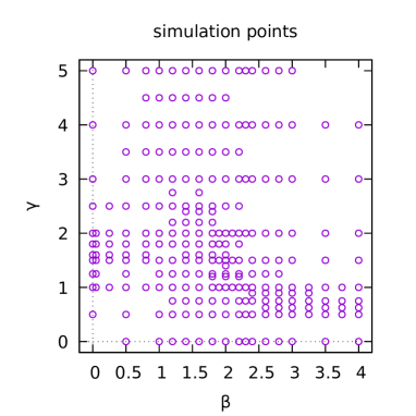
Figure 1: Simulation points in $\beta$-$\gamma$ plane.

The search for the phase boundary is performed by measuring the expectation value $\left\langle\mathcal{O}\right\rangle$ of a chosen operator $\mathcal{O}$ by changing $\gamma$ (or $\beta$) along the $\beta=$const. (or $\gamma=$const.) lines. In order to identify the boundary, we used the bent, step, and gap observed in the graph of the plots for $\left\langle\mathcal{O}\right\rangle$.

First of all, in order to determine the phase boundary of the model, we measure the Wilson action per plaquette (plaquette-action density),

$$P=\frac{1}{6N_{\text{site}}}\sum_{x}\sum_{\mu<\nu}\frac{1}{2}\mathrm{tr}(U_{x,\mu\nu}),\text{\qquad}U_{x,\mu\nu}=U_{x,\mu}U_{x+\hat{\mu},\nu}U_{x+\hat{\nu},\mu}^{{\dagger}}U_{x,\nu}^{{\dagger}}\text{, }$$ (16)

and that of the scalar action per link (scalar-action density),

$$M=\frac{1}{4N_{\text{site}}}\sum_{x}\sum_{\mu}\frac{1}{2}\mathrm{tr}\left(\left(D_{\mu}[U_{x,\mu}]\bm{\phi}_{x}\right)^{{\dagger}}\left(D_{\mu}[U_{x,\mu}]\bm{\phi}_{x}\right)\right)\text{, }$$ (17)

as Brower et al. have done in Brower82 .

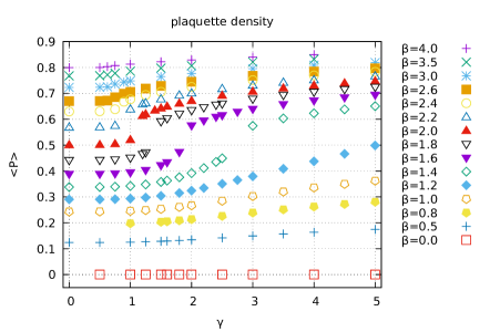
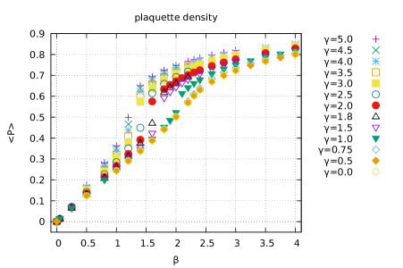
Figure 2: Average of the plaquette-action density $\left\langle P\right\rangle$: (Left) $\left\langle P\right\rangle$ versus $\gamma$ on various $\beta=$ const. lines, (Right) $\left\langle P\right\rangle$ versus $\beta$ on various $\gamma=$const. lines.

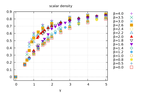
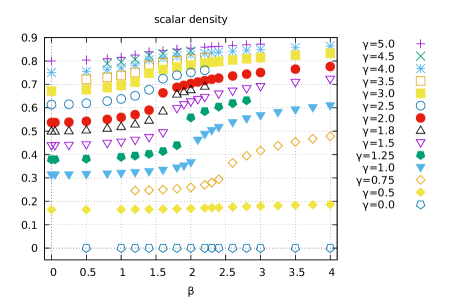
Figure 3: Average of the scalar-action density $\left\langle M\right\rangle$: (Left) $\left\langle M\right\rangle$ versus $\gamma$ on various $\beta=$ const. lines, (Right) $\left\langle M\right\rangle$ versus $\beta$ on various $\gamma=$const. lines.

First, we try to determine the phase boundary from the plaquette-action density. Fig.2 shows the results of measurements of the plaquette-action density $\left\langle P\right\rangle$ in the $\beta$–$\gamma$ plane. The left panel shows the plots of $\left\langle P\right\rangle$ along $\beta=$const. lines as functions of $\gamma$, where error bars are not shown because they are smaller than the size of the plot points. On the other hand, the right panel shows the plots of $\left\langle P\right\rangle$ along $\gamma=$const. lines as functions of $\beta$.

Next, in the same way, we try to determine the phase boundary from the scalar-action density. Fig.3 shows the results of measurement of the scalar-action density $\left\langle M\right\rangle$ in the $\beta$–$\gamma$ plane. The left panel of Fig.3 shows the plots of $\left\langle M\right\rangle$ along $\beta$-const. lines as functions of $\gamma$, while the right panel of Fig.3 shows the plots of $\left\langle M\right\rangle$ along $\gamma$-const. lines as functions of $\beta$.

In Fig.4, the phase boundary determined from the plaquette-action density $\left\langle P\right\rangle$ is given in the left panel of Fig.4. The phase boundary determined from the scalar-action density $\left\langle M\right\rangle$ is given in the right panel of Fig.4. The interval between the two simulation points corresponds to the short line with ends. The error bars in the phase boundary are due to the spacing of the simulation points. It should be noticed that the two phase boundaries determined from $\left\langle P\right\rangle$ and $\left\langle M\right\rangle$ are consistent within accuracy of numerical calculations. Thus we find that the gauge-independent numerical simulations reproduce the critical line obtained by Brower et al. Brower82 .

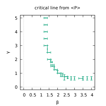
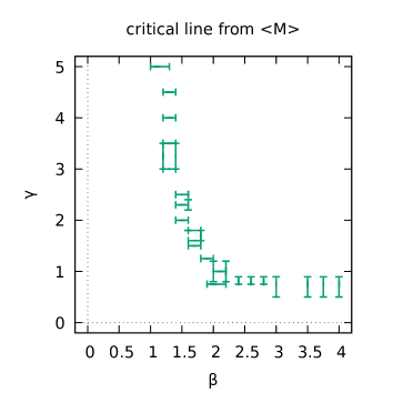
Figure 4: The phase boundary determined by the action densities: (Left) $\left\langle P\right\rangle$, (Right) $\left\langle M\right\rangle$.

III.2 Susceptibilities for $P$ and $M$

To find out more about phase boundary, we next measure “susceptibility” for the action densities:

$$\left\langle\chi(P)\right\rangle :=\left\langle P^{2}\right\rangle-\left\langle P\right\rangle^{2}\text{ ,}$$ (18)

$$\left\langle\chi(M)\right\rangle :=\left\langle M^{2}\right\rangle-\left\langle M\right\rangle^{2}\text{ .}$$ (19)

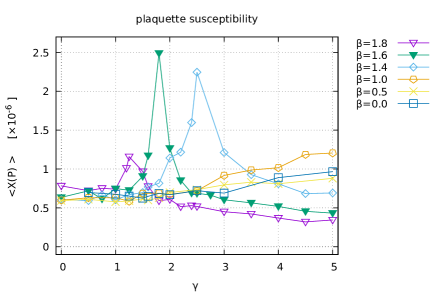
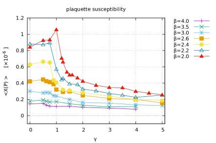
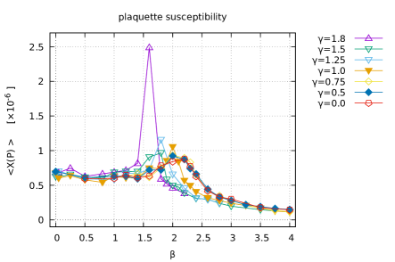
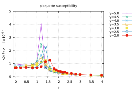
Figure 5: Susceptibility of plaquette $\left\langle\chi(P)\right\rangle$: (Upper panels) $\left\langle\chi(P)\right\rangle$ versus $\gamma$ on various $\beta=$const. lines, (Lower panels) $\left\langle\chi(P)\right\rangle$ versus $\beta$ on various $\gamma=$const. lines.

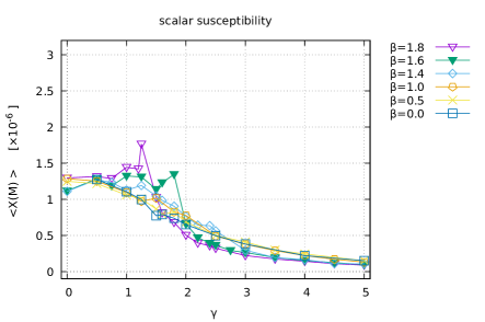
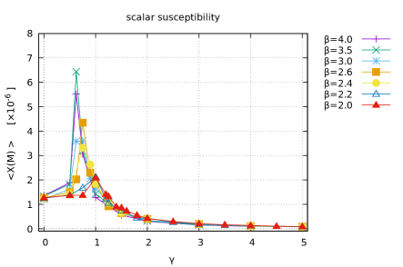
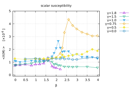
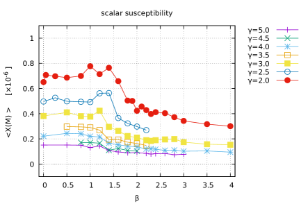
Figure 6: Susceptibility for the scalar-action $\left\langle\chi(M)\right\rangle$: (Upper panels) $\left\langle\chi(M)\right\rangle$ versus $\gamma$ on various $\beta=$const. lines, (Lower panels) $\left\langle\chi(M)\right\rangle$ versus $\beta$ on various $\gamma=$const. lines.

Figure 5 shows the measurements of $\left\langle\chi(P)\right\rangle$. The upper panels show plots of $\left\langle\chi(P)\right\rangle$ versus $\gamma$ along $\beta=$ const. lines, while the lower panels show plots of $\left\langle\chi(P)\right\rangle$ versus $\beta$ along the $\gamma=$ const. lines.

Figure 6 shows the measurements of $\left\langle\chi(M)\right\rangle$. The upper panels show plots of $\left\langle\chi(M)\right\rangle$ versus $\gamma$ along $\beta=$ const. lines, while the lower panels show plots of $\left\langle\chi(M)\right\rangle$ versus $\beta$ along the $\gamma=$ const. lines.

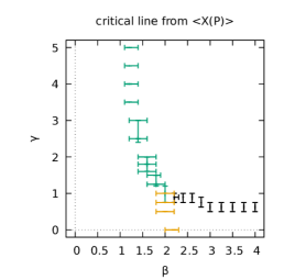
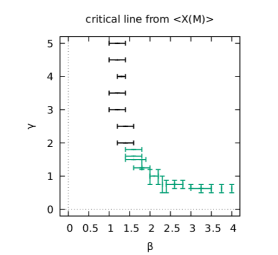
Figure 7: Critical lines determined from susceptibilities: (Left) from $\left\langle\chi(P)\right\rangle$, (Right) from $\left\langle\chi(M)\right\rangle$.

Figure 7 is the phase boundary determined by the susceptibility (specific heat) as a function of $\beta$ or $\gamma$. The green boundary is determined from the position of the peak in the susceptibility graph. The black boundary was determined from the position of the bend in the susceptibility graph. The orange boundary in the left panel of Fig. 7 is determined from the peak position of the plaquette-action susceptibility.

The left panel of Fig.7 gives same boundary as that determined by $\left\langle\chi(P)\right\rangle$ in Fig.4 for relatively large $\gamma$. However, the phase boundary in Fig.7 and Fig. 4 do not neccesarily coincide: in Fig.4 the boundary line in the region $\beta>2$ extends along the horizontal line $\gamma\simeq 1$ towards the pure scalar axis at $\beta=\infty$, while in the left panel of Fig.7 the boundary line extends also to the point $(\beta\simeq 2.2,\gamma=0)$ on the pure gauge axis at $\gamma=0$. This orange part of the phase boundary could be identified with the $SU(2)$ cross over in pure $SU(2)$ gauge theory which discriminates the weak coupling asymptotic scaling region from the strong coupling region, as seen by Bhanot and Creutz in their model BhanotCreutz81 .

The right panel of Fig.7 shows the phase boundary determined by measurements of $\left\langle\chi(M)\right\rangle$ given in Fig.6. The phase boundary determined from $\left\langle P\right\rangle$ and $\left\langle\chi(M)\right\rangle$ coincide. Note that graphs along $\gamma\approx 0.75$ and $\beta\approx$ $1.2$ corresponds to the cross sections along the ridge section of the phase boundary.

III.3 Correlations between the scalar field and the color-direction field through the gauge covariant decomposition

We measure the scalar-color correlation detected by the scalar-color composite operator:

$$Q=\frac{1}{N_{\text{site}}}\sum_{x}\frac{1}{2}\mathrm{tr}(\bm{n}_{x}\bm{\phi}_{x}),$$ (20)

where $\bm{n}_{x}$ is the color-direction field in the gauge-covariant decomposition for the gauge link variable. For this purpose, we need to solve the reduction condition (13) to obtain the color-direction field $\bm{n}_{x}$, which however has two kinds of ambiguity. One comes form so-called the Gribov copies that are the local minimal solutions of the reduction condition. In order to avoid the local minimal solutions and to obtain the absolute minima, the reduction condition is solved by changing the initial values to search for the absolute minima of the functional. The other comes from the choice of a global sign factor, which originates from the fact that whenever a configuration $\{\bm{n}_{x}\}$ is a solution, the flipped one $\{-\bm{n}_{x}\}$ is also a solution, since the reduction functional is quadratic in the color fields. To avoid these issues, we propose to use $\left\langle\left|Q\right|\right\rangle$ and $\left\langle Q^{2}\right\rangle$, which are examined as the order parameters that determine the phase boundary.

The phase boundary is searched for based on two ways:

(i)

the location at which $\left\langle\left|Q\right|\right\rangle$ changes from $\left\langle\left|Q\right|\right\rangle\simeq 0$ to $\left\langle\left|Q\right|\right\rangle>0$. This is also the case for $\left\langle Q^{2}\right\rangle$.

(ii)

the location at which $\left\langle\left|Q\right|\right\rangle$ changes abruptly, as was done for $\left\langle P\right\rangle$ and $\left\langle M\right\rangle$. This is also the case for $\left\langle Q^{2}\right\rangle$.

Figure 8 shows the measurements of $\left\langle\left|Q\right|\right\rangle$. The left panel shows plots of $\left\langle\left|Q\right|\right\rangle$ versus $\gamma$ along various $\beta=$const. lines, while the right panel shows plots of $\left\langle\left|Q\right|\right\rangle$ versus $\beta$ along various $\gamma=$const. lines.

Figure 9, on the other hand, shows the measurements of $\left\langle Q^{2}\right\rangle$ in the same manner as $\left\langle\left|Q\right|\right\rangle$.

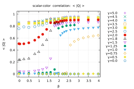
Figure 8: Average of the scalar-color composite field $\left\langle\left|Q\right|\right\rangle$: (Left) $\left\langle\left|Q\right|\right\rangle$ versus $\gamma$ on various $\beta=$const. lines, (Right) $\left\langle\left|Q\right|\right\rangle$ versus $\beta$ on various $\gamma=$const. lines.

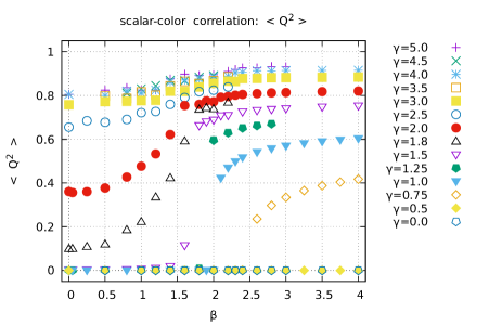
Figure 9: Average of the squared scalar-color composite field $\left\langle Q^{2}\right\rangle$: (Left) $\left\langle Q^{2}\right\rangle$ versus $\gamma$ on various $\beta=$const. lines, (Right) $\left\langle Q^{2}\right\rangle$ versus $\beta$ on various $\gamma=$const. lines.

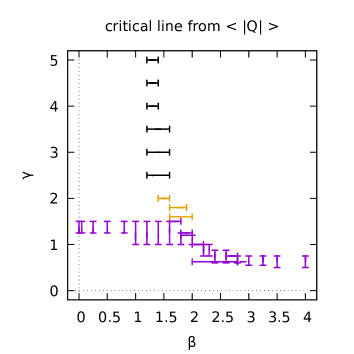
Figure 10: Critical lines determined (Left) from $\left\langle\left|Q\right|\right\rangle$, (Right) from $\left\langle Q^{2}\right\rangle$.

Figure 10 shows the phase boundary (critical line) determined by $\left\langle\left|Q\right|\right\rangle$ and $\left\langle Q^{2}\right\rangle$. The left panel of Fig.10 shows the phase boundary determined from $\left\langle\left|Q\right|\right\rangle$.

The purple boundary indicates that (i) $\left\langle\left|Q\right|\right\rangle$ changes from $\left\langle\left|Q\right|\right\rangle\simeq 0$ to $\left\langle\left|Q\right|\right\rangle>0$ (or $\left\langle Q^{2}\right\rangle$ changes from $\left\langle Q^{2}\right\rangle\simeq 0$ to $\left\langle Q^{2}\right\rangle>0$). The black boundary corresponds to the location at which $\left\langle\left|Q\right|\right\rangle$ (or $\left\langle Q^{2}\right\rangle$) has gaps. The orange boundary corresponds to the location at which $\left\langle\left|Q\right|\right\rangle$ (or $\left\langle Q^{2}\right\rangle$) bends. The right panel of Fig.10 shows the phase boundary determined from $\left\langle Q^{2}\right\rangle$. The results in Fig.10 are consistent with each other.

Fig.10 shows not only the phase boundary that divides the phase diagram into two phases, so-called the Higgs phase and the confinement phase, but also the new boundary that divides the confinement phase into two different parts. It should be remarked that this finding owes much to gauge-independent numerical simulations and their analyses, and this new results can only be established through our framework.

III.4 Susceptibility for the scalar and color-direction field

We finally investigate the “susceptibility” of the scalar-color local correlation:

$$\left\langle\chi(\left|Q\right|)\right\rangle=\left\langle Q^{2}\right\rangle-\left\langle\left|Q\right|\right\rangle^{2}$$ (21)

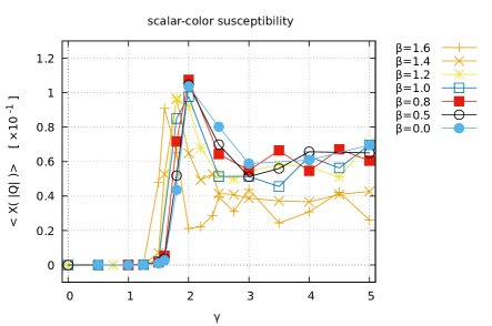
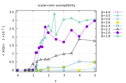
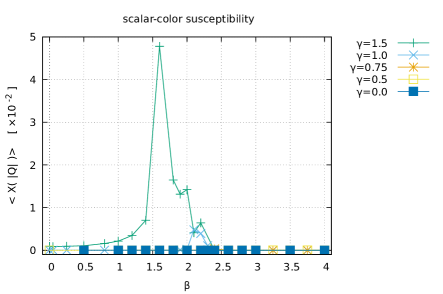
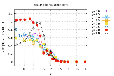
Figure 11: Susceptibility for the scalar-color field $\left\langle\chi(\left|Q\right|)\right\rangle$: (Upper panels) $\left\langle\chi(\left|Q\right|)\right\rangle$ versus $\gamma$ on various $\beta=$const. lines, (Lower panels) $\left\langle\chi(\left|Q\right|)\right\rangle$ versus $\beta$ on various $\gamma=$const. lines.

Figure 11 shows the measurement of $\left\langle\chi(\left|Q\right|)\right\rangle$. The upper panel of Fig.11 show plots of $\left\langle\chi(\left|Q\right|)\right\rangle$ versus $\gamma$ along the $\beta=$ const. lines and the lower panels show plots of $\left\langle\chi(\left|Q\right|)\right\rangle$ versus $\beta$ along the $\gamma=$const. lines.

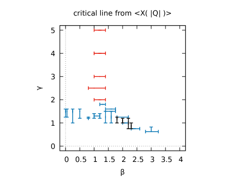
Figure 12: Critical line determined from the susceptibility $\left\langle\chi(\left|Q\right|)\right\rangle$.

First, we search for the transition along the vertical lines with fixed values of $\beta$ in a phase diagram. For relatively small fixed value of $\beta$ ($0\leq\beta\leq 1.6$), $\left\langle\chi(\left|Q\right|)\right\rangle$ is nearly equal to zero for small $\gamma$, but reaches a large but finite value across a critical value $\gamma_{c}(\beta)$, showing a peak as $\gamma$ increases. For larger values of $\beta$ ($1.8\leq\beta\leq 4.0$), $\left\langle\chi(\left|Q\right|)\right\rangle$ increases from zero to a finite value, which shows however no peak and increases monotonically as $\gamma$ increase. These observations yield the existence of a new transition line $\gamma=\gamma_{c}(\beta)$.

Next, we search for the transition along the horizontal line with fixed values of $\gamma$ in a phase diagram. For small fixed value of $\gamma$ ($0\leq\gamma\leq 1.5$), $\left\langle\chi(\left|Q\right|)\right\rangle$ shows nonzero value for small $\beta$, and decreases monotonically as $\beta$ increases.

Figure 12 shows the phase boundary (critical line) determined from $\left\langle\chi(\left|Q\right|)\right\rangle$. The blue boundary is obtained from the the location of the rapid change. The red and black intervals are obtained from the location of bends. This result agrees with the critical line already obtained in the above.

III.5 Understanding the new phase structure obtained from numerical simulations

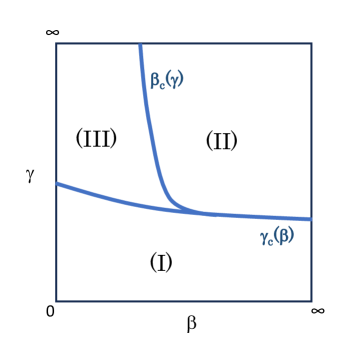
Figure 13: Phase structure of the lattice SU(2) gauge-adjoint scalar model: (I) Confinement phase, (II) Higgs phase, (III) Confinement phase.

Finally, we discuss why the above phase structure should be obtained and how the respective phase is characterized from the physical point of view. Figure 13 shows the schematic view of the resulting phase structure.

(i) First, we consider the region below the new critical line $\gamma<\gamma_{c}(\beta)$. In the limit $\gamma\to 0$, especially, the $SU(2)$ gauge-scalar model reduces to the pure compact $SU(2)$ gauge model which is expected to have a single confinement phase with no phase transition and has a mass gap on the whole $\beta$ axis in four spacetime dimensions Creutz82 . Confinement is expected to occur due to vacuum condensations of non-Abelian magnetic monopoles dualsuper . Here the non-Abelian magnetic monopole should be carefully defined gauge-independently using the gauge-invariant method, which is actually realized by extending the gauge-covariant decomposition of the gauge field, see KKSS15 for a review. More comments will be given below.

Even in the region $0<\gamma<\gamma_{c}(\beta)$, the effect of the scalar field would be relatively small and confinement would occur in the way similar to the pure $SU(2)$ gauge theory, which we call Confinement phase (I). Confinement phase (I) is regarded as a disordered phase in the sense that the color direction field $\bm{n}_{x}$ takes various possible directions with no specific direction in color space. This can be estimated through $Q$ in relation to the direction of the adjoint scalar field $\bm{\phi}_{x}$, which yields very small or vanishing values of the average $\langle Q\rangle=0$.

(ii) Next, we consider the region above the new critical line $\gamma>\gamma_{c}(\beta)$ where $\langle Q\rangle$ takes the non-vanishing value $\langle Q\rangle>0$, including the two phases: Higgs phase (II) $\gamma>\gamma_{c}(\beta)$, $\beta>\beta_{c}(\gamma)$ and Confinement phase (III) $\gamma>\gamma_{c}(\beta)$, $\beta<\beta_{c}(\gamma)$. In order to consider the difference between the two phases (II) and (III), we first consider the limit $\gamma\to\infty$. In this limit, the $SU(2)$ gauge-scalar model reduces to the pure compact $U(1)$ gauge model. The pure compact $U(1)$ gauge model in four spacetime dimensions has two phases: confinement phase with massive $U(1)$ gauge field in the strong gauge coupling region $\beta<\beta_{*}=\beta_{c}(\infty)$ and the Coulomb phase with massless $U(1)$ gauge field in the weak gauge coupling region $\beta>\beta_{*}=\beta_{c}(\infty)$, which has been proved rigorously Guth80 ; FS82 . Confinement in the compact $U(1)$ gauge model in the strong gauge coupling region $\beta<\beta_{*}=\beta_{c}(\infty)$ is understood based on the $U(1)$ magnetic monopole as shown in BMK77 .

For large but finite $\gamma<\infty$, furthermore, the critical line $\beta=\beta_{c}(\gamma)$ extends into the interior of the phase diagram from the critical point $(\beta_{*}=\beta_{c}(\infty),\gamma=\infty)$ as shown in Brower82 by integrating out the scalar field to obtain the effective gauge theory, which supports the above two regions even for finite $\gamma<\infty$.

In the Higgs phase (II): $\beta>\beta_{c}(\gamma)$ above the new critical line $\gamma>\gamma_{c}(\beta)$ with a finite $\gamma<\infty$, the off-diagonal gauge fields for the modes $SU(2)/U(1)$ become massive due to the BEH mechanism, which is a consequence of the (partial) spontaneous symmetry breaking $SU(2)\to U(1)$ according to the conventional understanding of the BEH mechanism, although this phenomenon is also understood gauge-independently based on the new understanding of the BEH mechanism without the spontaneous symmetry breaking Kondo16 . Therefore, the diagonal gauge field for the mode $U(1)$ always remains massless everywhere in the phase (II). This is not the case in the other phases. Therefore, the Higgs phase (II) can be clearly distinguished from the other phases. In the limit $\gamma\to\infty$, especially, the off-diagonal gauge fields become infinitely heavy and decouple from the theory, while the diagonal gauge field survives the limit both in (II) and (III). Consequently, the $SU(2)$ gauge-scalar model reduces to the pure compact $U(1)$ gauge model. This observation is consistent with the above consideration in the limit $\gamma\to\infty$.

The non-vanishing value $\langle Q\rangle>0$ means that the color-direction field $\bm{n}_{x}$ correlates strongly with the given scalar field $\bm{\phi}_{x}$ which tends to align to an arbitrary but a specific direction in this region $\gamma>\gamma_{c}(\beta)$ as expected from the spontaneous symmetry breaking in an ordered phase.

(iii) In the left region (III) $\beta<\beta_{c}(\gamma)$ above the new critical line $\gamma>\gamma_{c}(\beta)$ to be identified with another confinement phase (III), the gauge fields become massive due to different physical origins. In the region (III), indeed, the gauge fields become massive due to self-interactions among the gauge fields, as in the phase (I). In the confinement phase (III), no massless gauge field exists and the gauge fields for all the modes become massive, which is consistent with the belief that the original gauge symmetry $SU(2)$ would be kept intact and not spontaneously broken.

In the Confinement phases (I) and (III) there occur magnetic monopole condensations which play the dominant role in explaining quark confinement based on the dual superconductor picture, while in the Higgs phase (II) there are no magnetic monopole condensations and confinement would not occur. However, it should be remarked that the origin of magnetic monopoles is different in the two regions, (I) and (III). In (III) the magnetic monopole is mainly originated from the adjoint scalar field just like the ‘t Hooft-Polyakov magnetic monopole in the Georgi-Glashow model Polyakov77 . In (I) the magnetic monopole is constructed from the gauge field. Indeed, the magnetic monopole can be constructed only from the gauge degrees of freedom, which is explicitly constructed from the color direction field in the gauge-invariant way KKSS15 .

IV Conclusion and discussion

In this paper, we have investigated the lattice $SU(2)$ gauge-scalar model with the scalar field in the adjoint representation of the gauge group in a gauge-independent way. This model was considered to have two completely separated confinement and Higgs phases according to the preceding studies Brower82 based on numerical simulations which have been performed in the specific gauge fixing based on the conventional understanding of the Brout-Englert-Higgs mechanism Higgs1 .

We have re-examined this phase structure in the gauge-independent way based on the numerical simulations performed without any gauge fixing, which should be compared with the preceding studies Brower82 . This is motivated to confirm the recently proposed gauge-independent Brout-Englert-Higgs mechanics for giving the mass of the gauge field without relying on any spontaneous symmetry breaking Kondo16 ; Kondo18 . For this purpose we have investigated correlation functions between gauge-invariant operators obtained by combining the original adjoint scalar field and the new field called the color-direction field which is constructed from the gauge field based on the gauge-covariant decomposition of the gauge field due to Cho-Duan-Ge-Shabanov and Faddeev-Niemi.

Consequently, we have reproduced gauge-independently the transition line separating confinement and Higgs phase obtained in Brower82 , and show surprisingly the existence of a new transition line that divides completely the confinement phase into two parts. We have discussed the physical meaning of the new transition and implications to confinement mechanism. More discussions on the physical properties of the respective phase will be given in subsequent papers. In particular, it is quite important to study whether or not the new phase (III) is a lattice artefact and survives the continuum limit.

The result obtained in this paper should be compared with the lattice $SU(2)$ gauge-scalar model with the scalar field in the fundamental representation of the gauge group in a gauge-independent way. This model has a single confinement-Higgs phase where two confinement and Higgs regions are analytically continued according to the preceding studies Ostewlder78 ; FradkinShenker79 . Even in this case, it is shown Ikeda23 that the composite operator constructed from the original fundamental scalar field and the color-direction field can discriminate two regions and indicate the existence of the transition line seperating the confinement-Higg phase into completely different two phases, Confinement phase and Higgs phase.

Acknowledgement

This work was supported by Grant-in-Aid for Scientific Research, JSPS KAKENHI Grant Number (C) No.23K03406. The numerical simulation is supported by the Particle, Nuclear and Astro Physics Simulation Program No.2022-005 (FY2022) of Institute of Particle and Nuclear Studies, High Energy Accelerator Research Organization (KEK).

References

- (1) P.W. Higgs, Phys. Lett.12, 132 (1964). Phys. Rev. Lett. 13, 508 (1964). F. Englert and R. Brout, Phys. Rev. Lett.13, 321 (1964).
- (2) R.C. Brower, D.A. Kessler, T. Schalk, H. Levine, M. Nauenberg, Phys. Rev. D25, 3319 (1982).
- (3) S. Elitzur, Phys. Rev. D12, 3978 (1975).
- (4) K.-I. Kondo, Phys. Lett. B 762, 219 (2016). arXiv:1606.06194 [hep-th]
- (5) K.-I. Kondo, Eur. Phys. J. C 78, 577 (2018). arXiv:1804.03279 [hep-th]
- (6) Y.M. Cho, Phys. Rev. D21, 1080 (1980). Phys. Rev. D23, 2415 (1981).
- (7) Y.S. Duan and M.L. Ge, Sinica Sci. 11, 1072 (1979).
- (8) S.V. Shabanov, Phys. Lett. B463, 263 (1999). [hep-th/9907182]
- (9) L.D. Faddeev and A.J. Niemi, Phys. Rev. Lett. 82, 1624 (1999). [hep-th/9807069]; L.D. Faddeev and A.J. Niemi, Nucl. Phys. B776, 38 (2007). [hep-th/0608111]
- (10) A. Shibata, K.-I.Kondo, T.Shinohara, Phys. Lett.B691, 91 (2010). arXiv:0706.2529 [hep-lat]
- (11) A. Shibata, S. Kato, K.-I. Kondo, T. Murakami, T. Shinohara, S. Ito, Phys. Lett. B653, 101 (2007). arXiv:0706.2529 [hep-lat]
- (12) K.-I. Kondo, S. Kato, A. Shibata and T. Shinohara, Phys. Rept. 579, 1–226 (2015). arXiv:1409.1599 [hep-th]
-
(13)
Y. Nambu,
Phys. Rev. D10, 4262 (1974).
G. ’t Hooft, in: High Energy Physics, edited by A. Zichichi (Editorice Compositori, Bologna, 1975).
S. Mandelstam, Phys. Rept. 23, 245 (1976). - (14) G. Bhanot and M. Creutz Phys. Rev. D24, 3212 (1981).
- (15) M. Creutz, Quarks, Gluons and Lattices (Cambridge Monographs on Mathematical Physics) (Cambridge University Press, 1985).
- (16) A.H. Guth, Phys. Rev. D21, 2291 (1980).
- (17) J. Fröhlich and T. Spencer, Commun. Math. Phys. 83, 411 (1982).
- (18) T. Banks, R. Myerson, and J.B. Kogut, Nucl. Phys. B129, 493 (1977).
- (19) A.M. Polyakov, Nucl. Phys. B120, 429 (1977).
- (20) K. Ostewalder and E. Seiler, Annls. Phys 110, 440 (1978).
- (21) E. Fradkin and S.H. Shenker, Phys. Rev. D19, 3682 (1979).
- (22) R. Ikeda, S. Kato, K.-I. Kondo, and A. Shibata, Preprint CHIBA-EP-259, in preparation.