Entanglement in XYZ model on a spin-star system: Anisotropy vs. field-induced dynamics

Abstract

We consider a star-network of $n=n_{0}+n_{p}$ spin-$\frac{1}{2}$ particles, where interaction between $n_{0}$ central spins and $n_{p}$ peripheral spins are of the XYZ-type. In the limit $n_{0}/n_{p}\ll 1$, we show that for odd $n$, the ground state is doubly degenerate, while for even $n$, the energy gap becomes negligible when $n$ is large, inducing an effective double degeneracy. In the same limit, we show that for vanishing $xy$-anisotropy $\gamma$, bipartite entanglement on the peripheral spins computed using either a partial trace-based, or a measurement-based approach exhibits a logarithmic growth with $n_{p}$, where the sizes of the partitions are typically $\sim n_{p}/2$. This feature disappears for $\gamma\neq 0$, which we refer to as the anisotropy effect. Interestingly, when the system is taken out of equilibrium by the introduction of a magnetic field of constant strength on all spins, the time-averaged bipartite entanglement on the periphery at the long-time limit exhibits a logarithmic growth with $n_{p}$ irrespective of the value of $\gamma$. We further study the $n_{0}/n_{p}\gg 1$ and $n_{0}/n_{p}\rightarrow 1$ limits of the model, and show that the behaviour of bipartite peripheral entanglement is qualitatively different from that of the $n_{0}/n_{p}\ll 1$ limit.

I Introduction

Entangled quantum states Horodecki et al. (2009); *guhne2009 have been shown to be a key resource for several quantum technological applications including quantum communication Bennett and Wiesner (1992); *bennett1993; *mattle1996; *bouwmeester1997, quantum cryptography Ekert (1991); *jennewein2000; *Yin2020; *Schimpf2021, quantum simulation Dalmonte et al. (2018); *Kokail2021, quantum metrology Riedel et al. (2010); *Joo2011; *Demkowicz2014, measurement-based quantum computation Raussendorf and Briegel (2001); *briegel2009, and quantum algorithms Bruß and Macchiavello (2011). Being sources of entangled states, quantum many-body systems Amico et al. (2008); *Latorre2009; *dechiara2018 have been identified as candidate systems for implementing these applications. The last two decades have also witnessed the laboratory realization of quantum many-body Hamiltonians leading to quantum states possessing bipartite and multipartite entanglement using trapped ions Leibfried et al. (2003); *Porras2004; *Deng2005, nuclear magnetic resonance systems Vandersypen and Chuang (2005); *Rao2013, ultra-cold atoms and optical lattices Duan et al. (2003); *mandel2003; *bloch2005; *Treutlein2006; *Simon2011; *Cramer2013, and solid-state systems Schechter and Stamp (2008). This has made testing the theoretically predicted entanglement properties of these systems possible. From this motivation, interface of quantum information theory and quantum many-body systems has emerged as a vibrant field of research advancing along two complementary directions. On one hand, quantum technological applications have been implemented using quantum many-body systems, eg. quantum state transfer through spin chains Bose (2003); *Bose2013_chapter and one-way quantum computation Raussendorf and Briegel (2001); *briegel2009 using cluster states Hein et al. (2006). On the other hand, quantum information-theoretic concepts have been extensively used to probe quantum many-body systems Amico et al. (2008); *Latorre2009; *dechiara2018, leading to the introduction of projected entangled pair states Schollwöck (2005); *Verstraete2008; *Schollowck2011; *Orus2014; *Bridgeman_2017, and multiscale entanglement renormalization ansatz Verstraete and Cirac (2004); *Vidal2007; *Vidal2008; *Rizzi2008; *Aguado2008; *Cincio2008; *Evenbly2009.

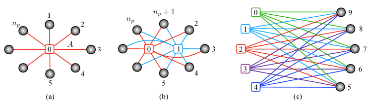
Figure 1: (Color online.) Star networks of $n=n_{0}+n_{p}$ spin-$\frac{1}{2}$ particles with (a) $n_{0}=1$ and (b) $n_{0}=2$, where peripheral spins are represented by shaded circles. As $n_{p}$ increases, the large periphery limit $n_{0}/n_{p}\ll 1$ is achieved, while an interchange of the central spins with the peripheral spins (i.e., an interchange between $n_{0}$ and $n_{p}$) provides the limit $n_{0}/n_{p}\gg 1$. The equal periphery limit of the system with $n_{0}/n_{p}=1$ is demonstrated with $n_{0}=n_{p}=5$ in (c). In these star networks, each spin in the periphery interacts with each of the central spin with XYZ interaction.

Among the variety of quantum many-body systems, interacting quantum spin models Amico et al. (2008); *Latorre2009; *dechiara2018 have attracted bulk of the attention due to their natural representation of multi-qubit or multi-qudit systems pertinent to quantum protocols. Although one- and two-dimensional regular lattices have primarily been in focus Amico et al. (2008); *Latorre2009; *dechiara2018, achievement of control over the connection between any two qubits in an array realized in different substrates Kane (1998); *Makhlin1999; *Imam1999; *Zheng2000; *Cirac2000 have also given rise to studies on quantum spin systems having a lattice structure modelled for specific purposes. Prime examples along this line of studies are (a) a star network of spins Hutton and Bose (2004), where a number of central spins are surrounded by a number of peripheral spins such that each of the central spin interacts with all of the peripheral spins (see Fig. 1 for examples with one and two central spin(s)), and (b) a star-chain network of spins, where a number of spin-chains have a common boundary spin Yao et al. (2011); *Ping2013; *ZHU2018; *Grimaudo2022. While such a network was originally envisioned for achieving control over entanglement through one, or a group of preferred (central) spins Hutton and Bose (2004), they have also been used as switch in quantum networks Yung (2011), in quantum state transfer and cloning Deng and Fang (2008), in magnetic resonance imaging Sushkov et al. (2014), in studying measurement uncertainty Haddadi et al. (2021), and to implement quantum heat engines T urkpence et al. (2017), refrigerators Arisoy and Müstecaplıoğlu (2021), and quantum batteries Liu et al. (2021); *Peng2021. The static and dynamical properties of entanglement Hutton and Bose (2004); Anzà et al. (2010); *Militello2011; *Ma2013; *He2019; *Karlova2023; Haddadi et al. (2019) in a star network of spins have also been extensively explored, along with the quantum correlations not belonging to the entanglement-separability paradigm Radhakrishnan et al. (2019); Haddadi et al. (2019) (cf. Modi et al. (2012); *bera2017).

In this paper, we consider a star-network of $n=n_{0}+n_{p}$ spins with $n_{0}$ central and $n_{p}$ peripheral spins, where each central (peripheral) spin interacts with each peripheral (central) spin via a fully anisotropic XYZ interaction Korepin et al. (1993); *Mila_2000; *Giamarchi2004; *Franchini2017. We consider three limits of the model – the large periphery limit given by $n_{0}/n_{p}\ll 1$, the large center limit given by $n_{0}/n_{p}\gg 1$, and the competing center limit, represented by $n_{0}/n_{p}\rightarrow 1$. In the large periphery limit, for non-zero values of the $xy$- and the $z$-anisotropy parameters, we investigate the structure of the ground state of the system. We show that for odd $n$, the ground states are doubly degenerate for all values of the anisotropy parameters. However, for even $n$, there is a finite energy gap between the ground and the first excited states for low and moderately high $n$. This energy gap decreases as $\exp{(-bn_{p}^{m})}$ for $\gamma=0$, and as $bn_{p}^{-m}$ for $\gamma\neq 0$ with increasing $n_{p}$, and the ground state becomes effectively doubly degenerate with a negligible energy gap once a critical size $n_{p}^{c}$ of the periphery (and hence, a critical size $n_{c}$ of the system) is achieved.

We next investigate the interplay of the bipartite entanglement over the peripheral spins and the size of the partitions in the zero-temperature and large periphery limits of the system. We take two separate approaches for quantifying bipartite entanglement in the periphery. One is the partial trace-based approach, where the central spins are traced out of the state of the system, leading to a mixed state on the peripheral spins which can be used to compute a bipartite entanglement measure over a pre-fixed bipartition of the peripheral spins Horodecki et al. (2009); *guhne2009. The other avenue is to localize DiVincenzo et al. (1998); Verstraete et al. (2004); *popp2005; Sadhukhan et al. (2017); *Krishnan2023; Banerjee et al. (2020); *Banerjee2022 non-zero average bipartite entanglement on the peripheral spins by performing a judiciously chosen projection measurement on the central spins. For both cases, we show that the bipartite entanglement over the equal bipartition of the peripheral spins exhibits a growth as $\log_{2}n_{p}$ with the periphery-size when the system has no $xy$-anisotropy (cf. Latorre et al. (2005); *Unanyan2005 for a similar finding in the Lipkin-Meshkov-Glick (LMG) model), while for non-zero $xy$-anisotropy, this feature is absent. We refer to this as the anisotropy effect. Moreover, for a fixed system-size $n$ with a partition-size $n^{\prime}$, both types of bipartite entanglement varies as $a\left[1-\exp\left(-b(n^{\prime})^{m}\right)\right]$.

Next, we consider taking the $n_{0}/n_{p}\ll 1$ limit of the system out of equilibrium by turning on a magnetic field of constant strength on all spins. As the system evolves, we calculate the bipartite entanglement from both approaches as a function of time at different points in the parameter space of the $xy$- and $z$-anisotropy parameters. The time-averaged bipartite entanglement corresponding to both approaches in the long-time limit are shown to have a logarithmic growth with $n_{p}$ for all values of the $xy$-anisotropy parameter, implying a negation of the anisotropy effect due to the field-induced dynamics. Also, similar to the static scenario, both types of average bipartite entanglement varies as $a\left[1-\exp\left(-b(n^{\prime})^{m}\right)\right]$ for a fixed $n_{p}$. We further consider the $n_{0}/n_{p}\gg 1$ and $n_{0}/n_{p}\rightarrow 1$ limits of the spin-star system, and find that the behaviours of bipartite peripheral entanglement in these limits are qualitatively different from the same for the $n_{0}/n_{p}\ll 1$ limit. In the case of $n_{0}/n_{p}\gg 1$, the bipartite peripheral entanglement decreases monotonically with increasing $n_{0}$ as $\sim bn_{0}^{-m}$, and vanishes asymptotically, while $n_{p}$ is kept fixed. For $n_{0}/n_{p}\rightarrow 1$, the bipartite peripheral entanglement saturates with $n_{p}$.

The rest of the paper is organized as follows. In Sec. II, we introduce the XYZ model on the spin-star system, and provide brief definitions of the partial trace-based and measurement-based approaches for quantifying bipartite entanglement on the peripheral spins. In Sec. III.1, we discuss the diagonalization of the system-Hamiltonian in the $n_{0}/n_{p}\ll 1$ limit, and explain the degeneracy and effective degeneracy of the ground state of the system for odd and even system sizes in Sec. III.2. The static properties of peripheral bipartite entanglement in the large periphery limit of the system is discussed in Sec. III.3, while the features of the dynamics of bipartite entanglement in the periphery due to the introduction of a magnetic field of constant magnitude is explored in Sec. III.4. The limits $n_{0}/n_{p}\gg 1$ and $n_{0}/n_{p}\rightarrow 1$ are discussed in Sec. III.5 and Sec. IV respectively. Sec. V contains the concluding remarks and outlook.

II Definitions

In this section, we set notations for describing the system, and present the necessary details for partial trace-based and measurement-based entanglement computed in the star network of spins.

II.1 Star network of spins

We consider a star-network Hutton and Bose (2004); Yung (2011); Deng and Fang (2008); Sushkov et al. (2014); Haddadi et al. (2021); T urkpence et al. (2017); Arisoy and Müstecaplıoğlu (2021); Liu et al. (2021); *Peng2021; Anzà et al. (2010); *Militello2011; *Ma2013; *He2019; *Karlova2023; Radhakrishnan et al. (2019); Haddadi et al. (2019) of $n=n_{0}+n_{p}$ spin-$1/2$ particles, where $n_{0}$ central spins are surrounded by $n_{p}$ peripheral spins such that each of the central spin interacts with all of the peripheral spins, but there is no interaction among the central spins and the peripheral spins themselves. Without any loss in generality, we label the central spins as $0,1,2,\cdots,n_{0}-1$, and the $n_{p}$ peripheral spins as $n_{0},n_{0}+1,n_{0}+2,\cdots,n_{0}+n_{p}-1$. We consider three limits of the model,

1. the large periphery limit, $n_{0}/n_{p}\ll 1$, where the size of the periphery is far larger than the size of the center,

2. the large center limit, $n_{0}/n_{p}\gg 1$, where the central spins outnumber the peripheral spins by a large number, and

3. the competing center limit, $n_{0}/n_{p}\rightarrow 1$, where the number of central spins is comparable to the number of peripheral spins.

See Fig. 1 for pictorial representations of these limits of the system. We assume each of the central spins $j$ interacting with all of the peripheral spins via the interaction Hamiltonian Korepin et al. (1993); *Mila_2000; *Giamarchi2004; *Franchini2017

$$H_{s} = K\sum_{i=0}^{n_{0}-1}\sum_{j=n_{0}}^{n_{0}+n_{p}-1}\left[(1+\gamma)S^{x}_{i}S^{x}_{j}+(1-\gamma)S^{y}_{i}S^{y}_{j}\right]$$ (1)

$$+\Delta K\sum_{i=0}^{n_{0}-1}\sum_{j=n_{0}}^{n_{0}+n_{p}-1}S^{z}_{i}S^{z}_{j},$$

Here, $i$ and $j$ are the spin indices corresponding to the central and the peripheral spins respectively, $S^{\alpha}_{i}=\sigma^{\alpha}_{i}/2$ is the standard representation of spin operators corresponding to the lattice site $i$, with $\sigma^{\alpha}$ being the Pauli matrices, $\alpha=x,y,z$, and $K$ is the strength of the exchange interaction. The dimensionless parameters $\gamma$ and $\Delta$ respectively represent the $xy$- and the $z$-anisotropy corresponding to all pairs of spins, with $-1\leq\gamma\leq 1$ and $-1\leq\Delta\leq 1$. The Hamiltonian $H_{s}$ represents a number of paradigmatic quantum spin Hamiltonians on the star network for different values of $\gamma$ and $\Delta$, including the XY model ($0<|\gamma|<1$, $\Delta=0$), the XX model ($\gamma=0,\Delta=0$) the classical Ising model ($\gamma=\pm 1$, $\Delta=0$), the isotropic Heisenberg model $(\gamma=0,\Delta=1)$, and the Heisenberg model with a $z$-anisotropy ($\gamma=0$, $0<|\Delta|<1$). In this paper, we consider the most general XYZ model ($0<|\gamma|<1$, $0<|\Delta|<1$) on the spin-star system in all three limits.

II.2 Entanglement in the star network of spins

To quantify entanglement in subsystems of the star network of spins in the state $\rho$, we consider two separate approaches, namely, (a) the partial trace-based approach, and (b) the measurement-based approach. The descriptions of these approaches are given below.

Partial trace-based approach.

Let us consider a bipartition $A:B$ of the system, where we aim to quantify entanglement in $B$. The size of the individual partitions $A$ and $B$ are respectively determined by the number of spins $N_{A}$ and $N_{B}$ in them. In the partial trace-based approach, the state $\rho_{B}$ on $B$ is determined by tracing out the spin degrees of freedom corresponding to all spins $a=1,2,\cdots,N_{A}$ in $A$, i.e.,

$$\rho_{B}=\text{Tr}_{A}[\rho].$$ (2)

Using $\rho_{B}$, a suitable bipartite or a multipartite entanglement measure $E_{B}=E(\rho_{B})$ is computed over the spins $b=1,2,\cdots,N_{B}$ in $B$ Horodecki et al. (2009); *guhne2009. In this paper, we consider the situation where $A$ is constituted only of the central spins, thereby having size $N_{A}=n_{0}$, while the peripheral spins constitute the partition $B$ of size $N_{B}=n_{p}$. We specifically focus on bipartite entanglement measures on $B$, and denote a bipartition of $B$ as $B_{1}:B_{2}$, with partitions $B_{1}$ and $B_{2}$ being of the sizes $n^{\prime}$ and $n_{p}-n^{\prime}$ respectively. For even $n_{p}$, $1\leq n^{\prime}\leq n_{p}/2$, while for odd $n_{p}$, $1\leq n^{\prime}\leq(n_{p}-1)/2$. Without any loss in generality, we assume that the spins $b=1,2,\cdots,n^{\prime}$ $\in B_{1}$, and $b=n^{\prime}+1,n^{\prime}+2,\cdots,n_{p}$ $\in B_{2}$. For clarity, we denote $E_{B}\equiv E_{B_{1}:B_{2}}$.

Measurement-based approach.

On the other hand, in the measurement based approach DiVincenzo et al. (1998); Verstraete et al. (2004); *popp2005; Sadhukhan et al. (2017); *Krishnan2023; Banerjee et al. (2020); *Banerjee2022, independent projection measurements are performed on all spins in $A$, giving rise to an ensemble of post-measured states

$$\varrho_{\mathbf{k}}=\frac{1}{p_{\mathbf{k}}}\left[(P_{A}^{\mathbf{k}}\otimes I_{B})\rho(P_{A}^{\mathbf{k}}\otimes I_{B})\right],$$ (3)

where each state $\varrho_{\mathbf{k}}$ has a probability of occurrence $p_{\mathbf{k}}=\text{Tr}\left[(P_{A}^{\mathbf{k}}\otimes I_{B})\rho(P_{A}^{\mathbf{k}}\otimes I_{B})\right]$, with $P_{A}^{\mathbf{k}}=\ket{\mathbf{k}}\bra{\mathbf{k}}$ being the projector corresponding to the measurement-basis $\ket{\mathbf{k}}$. For independent projection measurements on all spins in $A$,

$$P_{A}^{\mathbf{k}}=\otimes_{a\in A}\ket{\mathbf{k}_{a}}\bra{\mathbf{k}_{a}},$$ (4)

with $\mathbf{k}_{a}=\mathbf{0},\mathbf{1}$, where

$$\ket{\mathbf{0}_{a}} = \cos\frac{\theta_{a}}{2}\ket{0_{a}}+\text{e}^{\text{i}\phi_{a}}\sin\frac{\theta_{a}}{2}\ket{1_{a}},$$

$$\ket{\mathbf{1}_{a}} = \sin\frac{\theta_{a}}{2}\ket{0_{a}}-\text{e}^{\text{i}\phi_{a}}\cos\frac{\theta_{a}}{2}\ket{1_{a}},$$ (5)

$\{\ket{0_{a}},\ket{1_{a}}\}$ being the computational basis. For each measurement outcome $\mathbf{k}$ on $A$, the post-measured state $\varrho_{\mathbf{k}}$ has the form

$$\varrho_{\mathbf{k}}=P_{A}^{\mathbf{k}}\otimes\varrho_{B}^{\mathbf{k}},$$ (6)

so that an average entanglement over the ensemble of all possible post-measured states on $B$ can be defined as $\sum_{\mathbf{k}}p_{\mathbf{k}}E_{B}^{\mathbf{k}}$, with $E_{B}^{\mathbf{k}}=E(\varrho_{B}^{\mathbf{k}})$ is an entanglement measure, bipartite or multipartite, computed with the state $\varrho_{B}^{\mathbf{k}}$ on $B$. A maximization of $\langle E_{B}\rangle$ with respect to the $2N_{A}$ real parameters $\{\theta_{a},\phi_{a}\}$ $\forall a\in A$ leads to the definition of localizable entanglement Verstraete et al. (2004); *popp2005; Sadhukhan et al. (2017); *Krishnan2023; Banerjee et al. (2020); *Banerjee2022 over the subsystem $B$, given by

$$\langle E_{B}\rangle=\max_{\{\theta_{a},\phi_{a}\}}\left[\sum_{\mathbf{k}}p_{\mathbf{k}}E_{B}^{\mathbf{k}}\right],$$ (7)

via single-spin projection measurements over all spins in $A$. Similar to the case of the partial trace-based approach, we focus on bipartition $B_{1}:B_{2}$ in $B$, and write $E_{B}^{\mathbf{k}}=E_{B_{1}:B_{2}}^{\mathbf{k}}$, and $\langle E_{B}\rangle=\langle E_{B_{1}:B_{2}}\rangle$. Note that the basis-independence of partial trace and the convexity property Horodecki et al. (2009); *guhne2009 of the chosen entanglement measure $E$ implies

$$\langle E_{B_{1}:B_{2}}\rangle\geq E_{B_{1}:B_{2}}.$$ (8)

To quantify bipartite entanglement over a partition $B_{1}:B_{2}$ in a state $\rho_{B}$ (or $\varrho_{B}^{\mathbf{k}}$) on $B$, we use logarithmic negativity Plenio (2005) as an entanglement measure, defined as

$$\mathcal{L} = \log_{2}(\mathcal{N}+1),$$ (9)

where $\mathcal{N}$ is the negativity Peres (1996); *horodecki1996; *zyczkowski1998; *vidal2002; *lee2000 of $\rho_{B}$, defined as

$$\mathcal{N} = ||\rho_{B}^{T_{B_{1}}}||-1=2\left|\sum_{\lambda_{i}<0}\lambda_{i}\right|.$$ (10)

Here, $\rho_{B}^{T_{B_{1}}}$ is the partially transposed density matrix $\rho_{B}$ with respect to the subsystem $B_{1}$, $||.||$ denotes the trace norm, and $\lambda$ are the negative eigenvalues of $\rho_{B}^{T_{B_{1}}}$.

III XYZ model on a star network in the large periphery limit

We now consider the XYZ model on a star network of spins in the large periphery limit. We choose the case of a single central spin ($n_{0}=1$), and increase $n_{p}$ in order to attain this limit. We identify $|K|$ as the natural energy scale of the system, and write the dimensionless spin-star Hamiltonian $H_{s}/|K|\rightarrow H_{s}$ as

$$H_{s} = \pm\frac{1}{2}\left\{S_{0}^{+}(J_{p}^{-}+\gamma J_{p}^{+})+S_{0}^{-}(J_{p}^{+}+\gamma J_{p}^{-})\right\}$$ (11)

$$+\Delta S_{0}^{z}J_{p}^{z},$$

where $J_{p}^{\alpha}=\sum_{i=1}^{n_{p}}S^{\alpha}_{i}$, $\alpha=x,y,z$, are defined on the Hilbert space of the peripheral spins, and the signs of $H_{s}$ is determined by whether the spin-spin interaction is ferromagnetic (FM, $K>0$) or antiferromagnetic (AFM, $K<0$). Note that the operators $J_{p}^{\alpha}$, $\alpha=x,y,z$, obeys the usual commutation and anticommutation relation of angular momentum operators, implying that the peripheral spins collectively behave as a spin-$n_{p}/2$ particle with the spin operator $\mathbf{J}_{p}=(J_{p}^{x},J_{p}^{y},J_{p}^{z})$, while the total spin operator for the star network is given by $\mathbf{S}_{0}+\mathbf{J}_{p}$, with $\mathbf{S}_{0}=(S^{x}_{0},S^{y}_{0},S^{z}_{0})$. We also define $S^{\pm}_{i}=S^{x}_{i}\pm\text{i}S^{y}_{i}$ for the $i$th spin, and subsequently $J^{\pm}_{p}=\sum_{i=1}^{n_{p}}S^{\pm}_{i}$.

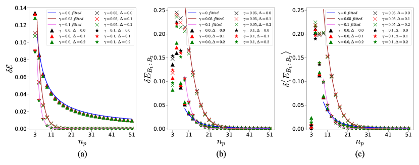
Figure 2: Variations of (a) $\delta\mathcal{E}$, (b) $\delta E_{B_{1}:B_{2}}$, and (c) $\delta\langle E_{B_{1}:B_{2}}\rangle$ as functions of $n_{p}$ for different values of $\gamma$ and $\Delta$, when $n$ is even. The fitting parameters corresponding to $\delta\mathcal{E}$ (Eq. (29)) and $\delta E_{B_{1}:B_{2}}$ and $\delta\langle E_{B_{1}:B_{2}}\rangle$ (Eq. (33)) can be found in Table 1 (see Appendix B). All quantities plotted are dimensionless.

III.1 Diagonalization

Since $[H_{s},\mathbf{J}_{p}^{2}]=[H_{s},\mathbf{S}_{0}^{2}]=0$, $H_{s}$ is block diagonal in the basis $\ket{b}=\ket{S_{0},m_{0}}\otimes\ket{J_{p},m_{p}}$, where

$$\mathbf{S}_{0}^{2}\ket{S_{0},m_{0}} = S_{0}(S_{0}+1)\ket{S_{0},m_{0}},$$

$$\mathbf{J}_{p}^{2}\ket{J_{p},m_{p}} = J_{p}(J_{p}+1)\ket{J_{p},m_{p}}.$$ (12)

Noticing that

1. $S_{0}$ only has one allowed value $S_{0}=\frac{1}{2}$ implying $m_{0}=\pm 1/2$, and

2. different blocks of $H_{s}$ corresponding to a fixed value of $m_{0}$ can be labelled by specific values of $J_{p}$, where $m_{p}$ in each block can take $2J_{p}+1$ values, $-J_{p}\leq m_{p}\leq J_{p}$,

for each block, it is sufficient to represent the basis as $\ket{b}=\ket{m_{0},m_{p}}=\ket{m_{0}}\otimes\ket{m_{p}}$. Evidently, the ground state of $H_{s}$ belongs to one of these blocks with a specific value of $J_{p}$. Our numerical analysis suggests that irrespective of the system size $n$, the ground state $\ket{\Psi_{0}}$ always belongs to the sector with $J_{p}=n_{p}/2$ (see, for example, Latorre et al. (2005); *Unanyan2005 for a similar property in the LMG model), while the same is true for the first excited state $\ket{\Psi_{1}}$ for $n_{p}\geq 3$ (see Appendix A for a demonstration with $n_{p}=2,3$).

Let us now set $\ket{m_{i}=\pm 1/2}$ basis as the computational basis $\{\ket{0}\equiv\ket{1/2},\ket{1}\equiv\ket{-1/2}\}$ for the spin $i$, such that

$$S^{z}_{i}\ket{+1/2} = (+1/2)\ket{+1/2},$$

$$S^{z}_{i}\ket{-1/2} = (-1/2)\ket{-1/2}.$$ (13)

Using this, we write the permutation-invariant Dicke state Sadhukhan et al. (2017); *Krishnan2023; Dicke (1954); *bergmann2013; *lucke2014; *kumar2017 on the $n_{p}$ peripheral spins with $n_{p}-l$ excitations:

$$\ket{D^{n_{p}}_{l}} = \frac{1}{\sqrt{\genfrac{(}{)}{0.0pt}{1}{n_{p}}{l}}}\sum_{i}\mathcal{P}_{i}\left(\ket{1}^{\otimes l}\ket{0}^{\otimes n_{p}-l}\right)$$ (14)

with the summation being over all possible permutations $\mathcal{P}_{i}$ over $n_{p}$-spin product states, where $l$ spins are in the ground state $\ket{1}$, and the rest $n_{p}-l$ spins are in the excited state $\ket{0}$, $0\leq l\leq n_{p}$. Noting that

$$J_{p}^{z}\ket{D_{l}^{n_{p}}} = \lambda_{l}\ket{D_{l}^{n_{p}}},$$ (15)

$$J_{p}^{2}\ket{D_{l}^{n_{p}}} = \lambda\ket{D_{l}^{n_{p}}},$$ (16)

$$J_{p}^{\pm}\ket{D_{l}^{n_{p}}} = \Big{[}\lambda-\lambda_{l}\left(\lambda_{l}\pm 1\right)\Big{]}^{\frac{1}{2}}\ket{D_{l\mp 1}^{n_{p}}},$$ (17)

where $\lambda_{l}=\frac{n_{p}}{2}-l$ and $\lambda=\frac{n_{p}}{2}\left(\frac{n_{p}}{2}+1\right)$, we further identify

$$\ket{D_{l}^{n_{p}}}\equiv\left|J_{p}=\frac{n_{p}}{2},m_{p}=\frac{n_{p}}{2}-l\right\rangle;\quad 0\leq l\leq n_{p}.$$ (18)

Therefore, the $J_{p}=n_{p}/2$ block of $H_{s}$, which we denote by $\mathcal{H}_{n_{p}/2}$, is a $2(n_{p}+1)$-dimensional subspace spanned by the permutation-invariant $n_{p}$ qubit Dicke states, with

$$\ket{m_{0},m_{p}}\equiv\ket{m_{0}}\otimes\ket{D^{n_{p}}_{l}};\quad 0\leq l\leq n_{p},$$ (19)

and $\mathcal{H}_{n_{p}/2}$ takes the form

$$\mathcal{H}_{n_{p}/2}=\begin{bmatrix}B&A\\ A^{T}&B^{\prime}\end{bmatrix},$$ (20)

with the matrix elements for the $n_{p}+1$ dimensional matrices $A$ and $B$ as

$$A_{i,j} = \left[\lambda-\lambda_{j}(\lambda_{j}-1)\right]^{\frac{1}{2}}\delta_{i-1,j}/2$$ (21)

$$+\gamma\left[\lambda-\lambda_{j}(\lambda_{j}+1)\right]^{\frac{1}{2}}\delta_{i+1,j}/2,$$

$$B_{i,j} = \Delta\lambda_{i}\delta_{i,j}/2=-B_{i,j}^{\prime},$$ (22)

where $i,j\in[0,n_{p}]$. Due to the linear increase in dimension with increasing $n_{p}$, $\mathcal{H}_{n_{p}/2}$ can be numerically diagonalized to obtain the ground state of the model even for large $n_{p}$.

We further re-arrange the basis corresponding to the subspace hosting $\mathcal{H}_{n_{p}/2}$ such that $\mathcal{H}_{n_{p}/2}$ takes the form

$$\mathcal{H}_{n_{p}/2} = \begin{bmatrix}A_{1}&0\\ 0&A_{2}\end{bmatrix},$$ (23)

where each of $A_{1},A_{2}$ are $(n_{p}+1)$-dimensional matrices, and the basis has been grouped as

$$A_{1} : \{\ket{+1/2}\ket{-n_{p}/2+2k},\ket{-1/2}\ket{-n_{p}/2+2k+1}\},$$

$$A_{2} : \{\ket{-1/2}\ket{-n_{p}/2+2k+1},\ket{+1/2}\ket{-n_{p}/2+2k}\},$$

with $0\leq k\leq n_{p}/2$ for even $n_{p}$, and $0\leq k\leq(n_{p}-1)/2$ when $n_{p}$ is odd. The utility of this re-arrangement will be clear in subsequent discussions.

III.2 On ground state degeneracy

Let us now define

$$\mathcal{O}=S_{0}^{x}\bigotimes_{i=1}^{n_{p}}S_{i}^{x},$$ (25)

where $[H_{s},\mathcal{O}]=0$. We first focus on the case of even $n_{p}$, and notice that $\mathcal{O}$ connects the basis elements corresponding to $A_{1}$ and that corresponding to $A_{2}$. Let us denote the eigenstate corresponding to the ground state energy $\mathcal{E}_{0}$ coming from $A_{1}$ is $\ket{\psi_{0}}_{A_{1}}$, and the same for $A_{2}$ is $\ket{\psi_{0}}_{A_{2}}$, while $\ket{\psi_{0}}_{A_{1}}=\mathcal{O}\ket{\psi_{0}}_{A_{2}}$, and vice-versa. The doubly-degenerate (DD) ground state of the system in the common eigenspace of $\mathcal{O}$ and $H_{s}$ is given by (see Appendix A for an example)

$$\ket{\Psi_{0}^{\pm}}=\frac{1}{\sqrt{2}}\left(\ket{\psi_{0}}_{A_{1}}\pm\ket{\psi_{0}}_{A_{2}}\right).$$ (26)

The double degeneracy in the ground state of $H_{s}$ is found for all the allowed values of $0\leq|\gamma|\leq 1$, and $0\leq|\Delta|<1$ when $n_{p}$ is even (i.e., when $n=n_{p}+1$ is odd).

On the other hand, in the case of odd $n_{p}$ (i.e., for even $n=n_{p}+1$), application of $\mathcal{O}$ on the eigenstates of $A_{1}$ ($A_{2}$) does not take the state out of the subspace of $A_{1}$ ($A_{2}$). Apart from the lines $|\Delta|=1$ in the $(\gamma,\Delta)$ parameter space where the ground state is DD (see Appendix A for examples), at all other allowed values of the anisotropy parameters ($0\leq|\gamma|<1$ and $0\leq|\Delta|<1$), the ground state in non-degenerate (ND). However, the energy gap $\delta\mathcal{E}=\mathcal{E}_{1}-\mathcal{E}_{0}$ of the system, $\mathcal{E}_{1}$ $(\mathcal{E}_{0})$ being the energy corresponding to the first excited (ground) state, decreases with increasing $n_{p}$ as (see Fig. 2)

$$\delta\mathcal{E} \sim \left\{\begin{array}[]{cc}a+bn_{p}^{-m}&\text{for }\gamma=0\\ a+\exp\left(-bn_{p}^{m}\right)&\text{for }\gamma\neq 0\end{array}\right.$$ (29)

where the parameters $a$, $b$ and $m$ can be obtained by fitting numerical data, as shown in Table 1 (see Appendix B). For $\gamma=0$, $\delta\mathcal{E}$ decreases slowly, and vanishes when the periphery-size $n_{p}$ is beyond a critical value $n_{p}^{c}\geq 5\times 10^{3}$ (i.e., when the system size is beyond a critical size $n_{c}=1+n_{p}^{c}$). This critical periphery-size, $n_{p}^{c}$, is a function of the chosen system parameters $(\gamma,\Delta)$. The collapse of $\delta\mathcal{E}\rightarrow 0$ becomes more rapid as the value of $\gamma$ increases, and is achieved for $n_{p}^{c}\geq 13$, when $\gamma\geq 10^{-1}$, while the effect of $\Delta$ on $n_{p}^{c}$ for a fixed $\gamma$ is nominal (see Fig. 3). For $n_{p}\geq n_{p}^{c}$ with odd $n_{p}$, the ground states of the system, denoted by $\ket{\Psi_{0}^{\pm}}$ for consistency with energy eigenvalues $\mathcal{E}_{1}$ and $\mathcal{E}_{0}$ respectively, can be considered to be effectively DD (EDD).

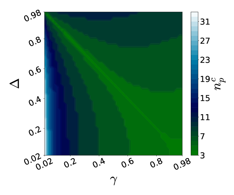
Figure 3: Variation of $n_{p}^{c}$ as a function of $\gamma$ and $\Delta$ in the ranges $0<\gamma,\Delta<1$. All quantities plotted are dimensionless.

Noticing the invariance of $H_{s}$ under permutation of spins on the periphery irrespective of the value of $n_{p}$, the general form of the ground state $\ket{\Psi_{0}}$ (degenerate, or non-degenerate), obtained from diagonalizing $\mathcal{H}_{n_{p}/2}$, can be written as

$$\ket{\Psi_{0}} = \sum_{l=0}^{n_{p}}\frac{c_{l}}{\sqrt{2}}\ket{\psi_{0}}\otimes\ket{D^{n_{p}}_{l}}+\sum_{l^{\prime}=0}^{n_{p}}\frac{d_{l^{\prime}}}{\sqrt{2}}\ket{\psi_{0}^{\perp}}\otimes\ket{D^{n_{p}}_{l^{\prime}}},$$

where $\sum_{l=0}^{n_{p}}|c_{l}|^{2}=\sum_{l^{\prime}=0}^{n_{p}}|d_{l^{\prime}}|^{2}=1$, and $\{\ket{\psi_{0}},\ket{\psi_{0}^{\perp}}\}$ constitute a complete orthonormal basis in the Hilbert space of the central spin. The coefficients $\{c_{l}\}$ and $\{d_{l^{\prime}}\}$ can be obtained by diagonalizing $\mathcal{H}_{n_{p}/2}$. If the ground state is doubly degenerate, one works with the thermal ground state (TGS) of $H_{s}$ Osborne and Nielsen (2002), given by an equal mixture of the degenerate ground states $\ket{\Psi_{0}^{\pm}}$ as

$$\rho_{0}=\frac{1}{2}\left(\ket{\Psi_{0}^{+}}\bra{\Psi_{0}^{+}}+\ket{\Psi_{0}^{-}}\bra{\Psi_{0}^{-}}\right).$$ (31)

In the case of EDD ground states occurring for large odd $n_{p}$, one can also work with $\rho_{0}$, and consider it as the effective TGS (ETGS), as there is negligible difference between $\mathcal{E}_{0}$ and $\mathcal{E}_{1}$.

III.3 Static entanglement properties: Anisotropy effect

In this paper, we are interested in the partial trace-based and measurement-based quantification of entanglement in $\ket{\Psi_{0}}$ (for ND ground state), or $\rho_{0}$ (for DD or EDD ground state). We note that tracing out the central spin from either of these two states leads to a state of the form

$$\rho_{p} = \sum_{l,l^{\prime}=0}^{n_{p}}c_{l,l^{\prime}}\ket{D^{n_{p}}_{l}}\bra{D^{n_{p}}_{l^{\prime}}},$$ (32)

for which prescription for computing entanglement $E_{B_{1}:B_{2}}$, quantified by the negativity or the logarithmic negativity, over arbitrary bipartition $B_{1}:B_{2}$ exists Stockton et al. (2003). On the other hand, a projection measurement on the central spin in the basis $\{\ket{0},\ket{1}\}$ results in a post-measured ensemble $\{\rho_{p}^{1},\rho_{p}^{2}\}$, with $\rho_{p}^{1,2}$ both being of the form (32), such that $\langle E_{B_{1}:B_{2}}\rangle$ can be computed. We point out here that the projection measurement on the central spin in the basis $\{\ket{0},\ket{1}\}$ may not be optimal, and would only provide a lower bound corresponding to the actual localizable entanglement (see Eq. (7)). However, our numerical analysis for small systems indicate that for $n_{0}\ll n_{p}$, $\{\ket{0},\ket{1}\}$ is the optimal basis.

Peripheral entanglement of EDD states.

Note that in the case of even $n_{p}$, the degenerate ground states $\ket{\Psi_{0}^{\pm}}$ are connected by the local unitary operator $\mathcal{O}$, and therefore have identical entanglement properties. However, this is not the case for odd $n_{p}$, and an interesting question would be how the two EDD states in the case of odd $n_{p}$ differ from each other in terms of values of $E_{B_{1}:B_{2}}$ and $\langle E_{B_{1}:B_{2}}\rangle$ where $n^{\prime}$ is typically fixed at $n^{\prime}=n_{p}/2$ for even $n_{p}$ ($n^{\prime}=(n_{p}-1)/2$ for odd $n_{p}$), when $n_{p}$ is increased. In Figs. 2(b), (c), we plot $\delta E_{B_{1}:B_{2}}=\left|E_{B_{1}:B_{2}}^{+}-E_{B_{1}:B_{2}}^{-}\right|$ and $\delta\langle E_{B_{1}:B_{2}}\rangle=\left|\langle E_{B_{1}:B_{2}}^{+}\rangle-\langle E_{B_{1}:B_{2}}^{-}\rangle\right|$ as functions of $n_{p}$ for different values of $\gamma$ and $\Delta$, where the $\pm$ in the superscripts in the expressions for $\delta E_{B_{1}:B_{2}}$ and $\delta\langle E_{B_{1}:B_{2}}\rangle$ denote the states $\ket{\Psi_{0}^{\pm}}$ (see discussions below Eq. (29)) for which entanglement is calculated. We find that $\delta E_{B_{1}:B_{2}}$ (and also $\delta\langle E_{B_{1}:B_{2}}\rangle$) approach zero as

$$\delta E_{B_{1}:B_{2}} \sim a+\exp\left(-bn_{p}^{m}\right),$$ (33)

similar to the $\gamma\neq 0$ case of Eq. (29) for the energy gap.

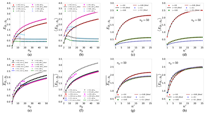
Figure 4: Variations of (a) $E_{B_{1}:B_{2}}$, (b) $\langle E_{B_{1}:B_{2}}\rangle$, (e) $\overline{E_{B_{1}:B_{2}}}$ and (f) $\overline{\langle E_{B_{1}:B_{2}}\rangle}$ as functions of $n_{p}$ for different values of $\gamma$, where $\Delta=0$ and $n^{\prime}=n_{p}/2$ ($(n_{p}-1)/2$) when $n_{p}$ is even (odd). The data for different $\gamma$ are fitted to Eq. (34) for (a)-(b) $n_{p}\geq 20$ and (e)-(f) $n_{p}\geq 24$. In (a)-(b) the values of $n_{p}^{c}$ are $n_{p}^{c}=4999$ for $\gamma=0$ (not shown in the figure), $n_{p}^{c}=19$ for $\gamma=0.05$, and $n_{p}^{c}=13$ for $\gamma=0.1$. We also plot the variations of (c) $E_{B_{1}:B_{2}}$, (d) $\langle E_{B_{1}:B_{2}}\rangle$, (g) $\overline{E_{B_{1}:B_{2}}}$ and (h) $\overline{\langle E_{B_{1}:B_{2}}\rangle}$ with $n^{\prime}$ where $\gamma$ is varied and $\Delta=0$, $n_{p}=50$. The data are fitted to Eq. (35). The fitting parameters are provided in Table 1 (see Appendix B). All quantities plotted are dimensionless.

Peripheral entanglement against system-size.

We now discuss the features of $E_{B_{1}:B_{2}}$ and $\langle E_{B_{1}:B_{2}}\rangle$ in the case of the XYZ model in the star network of spins with $n_{0}=1$. For demonstration, we choose $n^{\prime}=n_{p}/2$ (for even $n_{p}$), and $(n_{p}-1)/2$ (for odd $n_{p}$). Fig. 4(a)-(b) depicts the variations of $E_{B_{1}:B_{2}}$ and $\langle E_{B_{1}:B_{2}}\rangle$ as functions of $n_{p}$ for different values of $\gamma$ and $\Delta$. The qualitative features of the partial trace-based and the measurement-based entanglement are similar, as indicated from Fig. 4. It is important to note that on the $(\gamma,\Delta)$ plane for odd $n_{p}$, the onset of $\delta\mathcal{E}=0$ (i.e., $n_{p}^{c}$) is different for different points. This is indicated by the discontinuities in the variations of entanglement for odd $n_{p}$, computed from the ND ground state $\ket{\Psi_{0}}$ (Eq. (LABEL:eq:ground_state_form)) for $n_{p}\leq n_{p}^{c}$, and from the mixed ETGS $\rho_{0}$ (Eq. (31)) for $n_{p}>n_{p}^{c}$. For $\gamma=0$, $E_{B_{1}:B_{2}}$ (and also $\langle E_{B_{1}:B_{2}}\rangle$) exhibit a logarithmic dependence on $n_{p}$ as

$$E_{B_{1}:B_{2}} \sim a+b\log_{2}n_{p},$$ (34)

where the fitting parameters $a$ and $b$ can be obtained by fitting the data for $E_{B_{1}:B_{2}}$ and $\langle E_{B_{1}:B_{2}}\rangle$ against $n_{p}$ (see Fig. 4(a)-(b) for the example of $\Delta=0$) when $n_{p}>n_{p}^{c}$. Also our numerical analysis suggest that for $\gamma=0$, $a$ and $b$ depends on the choice of $\Delta$ weakly for even $n_{p}$, and are independent of $\Delta$ for odd $n_{p}$. However, in stark contrast, the logarithmic dependence is absent for $\gamma\neq 0$. This result indicate a prominent change in the variations of $E_{B_{1}:B_{2}}$ and $\langle E_{B_{1}:B_{2}}\rangle$ with periphery-size for vanishing and non-vanishing anisotropy parameter $\gamma$. We refer to this as the anisotropy effect. We point out here that this feature is unchanged for all constant ratios $n^{\prime}/n_{p}$ , where for the logarithmic dependence on $n_{p}$ in case of $\gamma=0$, only values of $a$ and $b$ change.

For a fixed periphery-size $n_{p}$ (and subsequently for a fixed system-size $n$) and a varying partition size $n^{\prime}$ where the maximum value of $n^{\prime}$ is typically $n_{p}/2$, for all $\gamma$, $E_{B_{1}:B_{2}}$ (and $\langle E_{B_{1}:B_{2}}\rangle$) vary as

$$E_{B_{1}:B_{2}} \sim a\left[1-\exp\left(-b(n^{\prime})^{m}\right)\right],$$ (35)

which is demonstrated in Figs. 4(c)-(d) for both types of entanglement. Note that for $\gamma=0$, the fitting parameters $a,b$ and $m$ remains unaffected up to three decimal places for $\langle E_{B_{1}:B_{2}}\rangle$ when $0\leq\Delta<1$. For $E_{B_{1}:B_{2}}$, fitting parameter $a$ has slight dependence on $\Delta$ which changes even the first decimal place. Whereas fitting parameters $b$ and $c$ remain unchanged up to two and three decimal places respectively. On the other hand, for $\gamma\neq 0$, all the fitting parameters depends on $\Delta$.

Figure 5: A typical snapshot of the time-variations of $E_{B_{1}:B_{2}}$ and $\langle E_{B_{1}:B_{2}}\rangle$. The horizontal lines represent $\overline{E_{B_{1}:B_{2}}}$ and $\overline{\langle E_{B_{1}:B_{2}}\rangle}$. All quantities plotted are dimensionless.

III.4 Field-induced dynamics of entanglement

We now consider a situation where a time-dependent local magnetic field of strength $f(t)$ is applied to all spins in the star network. The field strength is such that

$$f(t)=\left\{\begin{array}[]{cc}0;&t=0\\ h;&t>0\end{array}\right.,$$ (38)

where $h>0$ (see Barouch et al. (1970); *Barouch1971; *Barouch1971a; Chanda et al. (2016) for use of similar magnetic field). The system at $t>0$ therefore evolves in time due to the time-independent Hamiltonian

$$H_{\text{tot}}=H_{s}+h\sum_{i=0}^{n_{0}+n_{p}-1}S_{i}^{z},$$ (39)

where we redefine $h\rightarrow h/|K|$ to keep $H_{\text{tot}}$ dimensionless. Note that the features of block-diagonalization of $H$ discussed in Sec. III.1 remain unchanged for $H_{\text{tot}}$ also, irrespective of the value of $h$.

Starting from an initial state $\rho_{0}$ of the system, the time-evolved state of the full system at time $t$ is given by

$$\rho(t)=\text{e}^{-\text{i}H_{\text{tot}}t}\rho_{0}\text{e}^{\text{i}H_{\text{tot}}t}.$$ (40)

The time-dependence of the partial trace-based entanglement on the peripheral qubits can be computed using $\rho_{p}(t)=\text{Tr}_{0}\rho(t)$, while the measurement-based entanglement can be computed by performing single-qubit projective measurements on the central qubit, when the system is in state $\rho(t)$. In Fig. 5, we plot the time-evolution of $E_{B_{1}:B_{2}}$ and $\langle E_{B_{1}:B_{2}}\rangle$ for a system with $n_{p}=30$ , and $n^{\prime}=15$. Both $E_{B_{1}:B_{2}}$ and $\langle E_{B_{1}:B_{2}}\rangle$ oscillate with $t$, and the average values, $\overline{E_{B_{1}:B_{2}}}$ and $\overline{\langle E_{B_{1}:B_{2}}\rangle}$, are obtained by averaging over the time-series data in the long-time limit. We probe the long-time limit of the time-evolving spin-star system using $\overline{E_{B_{1}:B_{2}}}$ and $\overline{\langle E_{B_{1}:B_{2}}\rangle}$. Note that for $\gamma=0$, the field term commutes with the Hamiltonian irrespective of $\Delta$, leading to no time-evolution of the initial state. Therefore, we specifically focus on the cases with $\gamma\neq 0$. In Figs. 4(e) and (f), we respectively plot $\overline{E_{B_{1}:B_{2}}}$ and $\overline{\langle E_{B_{1}:B_{2}}\rangle}$ as functions of $n_{p}$, where the partition-size $n^{\prime}=n_{p}/2$ $((n_{p}-1)/2)$ for even (odd) $n_{p}$. In contrast to the static case discussed in Sec.III.3, for large $n_{p}$, both $\overline{E_{B_{1}:B_{2}}}$ and $\overline{\langle E_{B_{1}:B_{2}}\rangle}$ exhibit logarithmic growth with $n_{p}$ in both $xy$-isotropic ($\gamma=0$) and $xy$-anisotropic ($\gamma\neq 0$) conditions, thereby negating the anisotropy effect. The discrepancies in the logarithmic variation due to the finite-size of the system vanishes within $n_{p}\sim 20$. We further test the variations of $\overline{E_{B_{1}:B_{2}}}$ and $\overline{\langle E_{B_{1}:B_{2}}\rangle}$ with $n^{\prime}$ for a fixed $n_{p}$, and found them to be similar to the static case (see Eq. (35)). See Figs. 4(g)-(h).

III.5 Large center limit

We now consider the XYZ model on the star network of spins when the size of the center is far larger than the size of the periphery, i.e., $n_{0}/n_{p}\gg 1$. Note that this limit is identical to the $n_{0}/n_{p}\ll 1$ limit of the model through an interchange of the central spins with peripheral spins, thereby exhibiting similar features of ground state energy as the limit $n_{0}/n_{p}\ll 1$. We present the variation of $E_{B_{1}:B_{2}}$ with $n_{0}$ for a fixed $n_{p}$ in the limit $n_{0}/n_{p}\gg 1$ in Fig. 6(a) (the minimal instance of two peripheral spins and $n_{p}$ central spins is represented in Fig. 1(b)). Our numerical analysis suggests that in contrast to the results obtained in the limit $n_{0}/n_{p}\ll 1$, for increasing $n_{0}$ with $n_{0}/n_{p}\gg 1$, $E_{B_{1}:B_{2}}$ decreases monotonically and approaches zero asymptotically as

$$E_{B_{1}:B_{2}}\sim a+bn_{0}^{-m},$$ (41)

where the fitting parameters are obtained from the numerical data (see Fig. 6(a)).

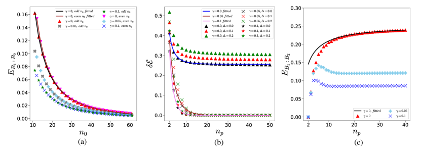
Figure 6: (a) Variation of $E_{B_{1}:B_{2}}$ with $n_{0}$ in the limit $n_{0}/n_{p}\gg 1$, where $n_{p}$ is fixed at $n_{p}=10$. For $\gamma=0$, the data is fitted to Eq. (41). (b)-(c) Variations of (b) $\delta\mathcal{E}$ and (c) $E_{B_{1}:B_{2}}$ with $n_{p}$ in the limit $n_{0}/n_{p}\rightarrow 1$, where we fix $n_{0}=n_{p}$. The data corresponding to $\Delta=0$ in (b) are fitted to Eq. (43), while the same corresponding to $\gamma=0$ in (c) are fitted to Eq. (45). See Table 1 ( Appendix B)for the numerical values of the respective fitting parameters. All quantities plotted are dimensionless.

IV XYZ model on a star network in the competing center limit

A question that naturally arises at this point is whether the features of bipartite peripheral entanglement remain the same as one considers the limit $n_{0}/n_{p}\rightarrow 1$. In this situation, the dimensionless spin-star Hamiltonian is given by (see Eq. (11))

$$H_{s} = \pm\frac{1}{2}\Big{[}J_{0}^{+}(J_{p}^{-}+\gamma J_{p}^{+})+J_{0}^{-}(J_{p}^{+}+\gamma J_{p}^{-})+\Delta J_{0}^{z}J_{p}^{z}\Big{]},$$

where $J_{0}^{\pm}=\sum_{i=0}^{n_{0}-1}S_{i}^{\pm}$, $J_{0}^{z}=\sum_{i=0}^{n_{0}-1}S_{i}^{z}$, $J_{p}^{\pm}=\sum_{i=n_{0}}^{n_{0}+n_{p}-1}S_{i}^{\pm}$, and $J_{p}^{z}=\sum_{i=n_{0}}^{n_{0}+n_{p}-1}S_{i}^{z}$. Analysis for the Hamiltonian (LABEL:eq:Hamiltonian_coupled_central) is similar to that of the Hamiltonian (11) in the case of the single central spin, and the values of $J_{0}$ and $J_{p}$ corresponding to the ground and the first excited states of $H_{s}$ are $n_{0}/2$ and $n_{p}/2$ respectively, independent of the system parameters $\gamma$, and $\Delta$. Upon diagonalization, doubly degenerate ground states are found when $n=n_{0}+n_{p}$ is odd irrespective of the values of $(\gamma,\Delta)$, while the effective degeneracy in ground states for large system size is observed when $n$ is even only for $\gamma\neq 0$ (see Fig. 6(b)). Note that in the present case, $\delta\mathcal{E}$ approaches saturation (for $\gamma=0$) or vanishing (for $\gamma\neq 0$) as

$$\delta\mathcal{E}\sim a+\exp\left(-bn_{p}^{m}\right).$$ (43)

For $\gamma=0$, according to our numerical investigation up to $n_{p}=n_{0}=50$, $\delta\mathcal{E}$ saturates to a non-zero value, which increases with an increase in the value of $\Delta$, implying a ND ground state for $\gamma=0$ up to the maximum system-size investigated in this paper.

In the limit $n_{0}/n_{p}\rightarrow 1$, the structure of the ground states with permutation symmetry in both central and peripheral qubits is given by

$$\ket{\Psi_{0}} = \sum_{l^{\prime}=0}^{n_{0}}\sum_{l=0}^{n_{p}}c_{l,l^{\prime}}\ket{D_{l^{\prime}}^{n_{0}}}\otimes\ket{D^{n_{p}}_{l}},$$ (44)

where $\sum_{l^{\prime}}\sum_{l}|c_{l,l^{\prime}}|^{2}=1$, and the definition of $\ket{D_{l^{\prime}}^{n_{0}}}$ is similar to that of $\ket{D_{l}^{n_{p}}}$. Similar to the case of single central qubit, the TGS $\rho_{0}$ corresponding to the degenerate and the effectively degenerate ground states $\ket{\Psi^{\pm}_{0}}$ is of the form (31), while the mixed state $\rho_{p}$ on the peripheral qubits obtained via tracing out the central qubits is of the form (32), enabling one to compute the bipartite entanglement $E_{B_{1}:B_{2}}$ on the peripheral spins. In Fig. 6(c), we plot the variations of $E_{B_{1}:B_{2}}$ as a function of $n_{p}$, where $n_{p}=n_{0}$. In contrast to the limit $n_{0}/n_{p}\ll 1$, $E_{B_{1}:B_{2}}$ for $\gamma=0$ saturates with increasing $n_{p}$ as

$$E_{B_{1}:B_{2}} \sim a\left[1-\exp\left(-bn_{p}^{m}\right)\right].$$ (45)

For $\gamma\neq 0$ also, $E_{B_{1}:B_{2}}$ saturates with $n_{p}$, although the approach to saturation is different from that of the $\gamma=0$, and the saturation value decreases with increasing $\gamma$, implying an anisotropy effect. However, the time-averaged bipartite peripheral entanglement, $\overline{E_{B_{1}:B_{2}}}$, in contrast to the $n_{0}/n_{p}\ll 1$ limit, does not negate the anisotropy effect.

V Conclusion and Outlook

In this paper, we study the XYZ model on a spin-star system, where a number of central spins are connected to a number of peripheral spins in such a way that each central spin interacts with all peripheral spins. We specifically consider the limit of the system where the number of central spins are very small compared to the number of peripheral spins. In this limit, the ground state of the system is doubly degenerate when the system-size is even, while there is a finite energy gap between the ground and the first excited states of the system with odd number of spins. This energy gap decreases rapidly with increasing system-size, inducing an effective double degeneracy of the ground states. When the system size is large (i.e., when the periphery-size is large), the bipartite entanglement over typically equal bipartition of the periphery, computed from either partial trace-based, or measurement-based approaches, exhibits a logarithmic growth with the periphery-size when the system is $xy$-isotropic (i.e., $\gamma=0$). This feature vanishes for $\gamma\neq 0$, which we refer to as the anisotropy effect. Interestingly, the anisotropy effect can be nullified by kick-starting a magnetic field of constant strength on all spins in the system, where the average values of the time-series of bipartite peripheral entanglement computed from either of the approaches exhibit a logarithmic growth with the periphery-size irrespective of the values of $\gamma$. We further consider the large center and the competing center limits of the model, and find the features of bipartite peripheral entanglement to be qualitatively different from that of the large periphery limit of the model.

A number of possible research directions open up from this study. Within the range of the results reported in this paper, it would be interesting to investigate whether similar features in entanglement exists if interactions are present within the central and/or the peripheral spins themselves. Also, a similar investigation in a star-chain configuration of spin-$\frac{1}{2}$ particles Yao et al. (2011); *Ping2013; *ZHU2018; *Grimaudo2022 is yet to be performed. Another interesting question would be whether these entanglement properties of the spin-star system are robust against the presence of quenched disorder in the system De Dominicis and Giardina (2006). Besides, similarity of our results with the already existing results for the LMG model Latorre et al. (2005); *Unanyan2005 raises the question as to what would be the underlying principle to model a spin-lattice system that exhibits similar entanglement properties. Moreover, recent interests in exploring quantum technological aspects involving $d$-level systems, or qudits Wang et al. (2020) highlights the relevance of exploring similar models where lattice sites are populated with spins having a higher spin quantum number.

Appendix A Small systems with single central spin

In this section, we look into two specific examples for $n_{p}=2$ and $n_{p}=3$ in the case of a star network of $(n_{p}+1)$ spins, as follows.

A.1 $n_{p}=2$

We first consider the case of $J_{p}=1$ ($m_{p}=-1,0,1$) among the allowed values $J_{p}=0,1$ for $n_{p}=2$. We group the basis states according to Eq. (LABEL:eq:grouping) as

$$\{\ket{-1/2}\ket{-1},\ket{1/2}\ket{0},\ket{-1/2}\ket{1}\}$$

and

$$\{\ket{1/2}\ket{-1},\ket{-1/2}\ket{0},\ket{1/2}\ket{1}\}$$

respectively, leading to the $\mathcal{H}_{1}$ block having the form (23), with $A_{1}$ and $A_{2}$ being two $3\times 3$ matrices given by

$$A_{1} = \frac{1}{2}\begin{bmatrix}-\Delta&0&\alpha^{-}_{0}\\ 0&\Delta&\gamma\alpha^{+}_{0}\\ \alpha^{+}_{-1}&\gamma\alpha^{-}_{1}&0\end{bmatrix},$$ (46)

$$A_{2} = \frac{1}{2}\begin{bmatrix}0&\gamma\alpha^{+}_{-1}&\alpha^{-}_{1}\\ \gamma\alpha^{-}_{0}&\Delta&0\\ \alpha^{+}_{0}&0&-\Delta\end{bmatrix},$$ (47)

upto a normalization factor, where

$$\alpha^{\pm}_{m_{p}}=\sqrt{J_{p}(J_{p}+1)-m_{p}(m_{p}\pm 1)}.$$ (48)

Note that $|A_{1}|=|A_{2}|=2\Delta(\gamma^{2}-1)$, which vanishes for $\Delta=0$ or $\gamma=\pm 1$, implying that at least one of the eigenvalues of both $A_{1}$ and $A_{2}$ vanishes at these conditions. For $\Delta=0$, the eigenvalues are $0,\pm\sqrt{2(\gamma^{2}+1)}/2$ for both $A_{1}$ and $A_{2}$, leading to the doubly-degenerate ground state energy $-\sqrt{2(\gamma^{2}+1)}/2$. The corresponding eigenvectors belonging to the blocks $A_{1}$ and $A_{2}$ are given by

$$\ket{\psi}_{0,{A_{1}}} = \frac{1}{\sqrt{2(\gamma^{2}+1)}}\ket{-1/2}_{0}\Big{(}\ket{-1}_{p}+\gamma\ket{1}_{p}\Big{)}$$

$$-\frac{1}{\sqrt{2}}\ket{1/2}_{0}\ket{0}_{p},$$

$$\ket{\psi}_{0,{A_{2}}} = \frac{1}{\sqrt{2(\gamma^{2}+1)}}\ket{1/2}_{0}\Big{(}\gamma\ket{-1}_{p}+\ket{1}_{p}\Big{)}$$ (49)

$$-\frac{1}{\sqrt{2}}\ket{-1/2}_{0}\ket{0}_{p},$$

where clearly $\ket{\psi}_{0,A_{1}}=\mathcal{O}\ket{\psi}_{0,A_{2}}$, and vice-versa (see Sec. III.2). Consequently, the doubly degenerate ground-states corresponding to the ground-state energy $-\sqrt{2(\gamma^{2}+1)}/2$ and in the common eigenspace of $H_{s}$ and $\mathcal{O}$ are given by Eq. (26). Similarly for $\gamma=\pm 1$, the eigenvalues of either of $A_{1}$ and $A_{2}$ are $0,\pm\sqrt{4+\Delta^{2}}/2$, with the doubly-degenerate ground state energy $-\sqrt{4+\Delta^{2}}/2$, and the corresponding eigenvectors being

$$\ket{\psi}_{0,{A_{1}}} = \Big{(}\frac{\sqrt{4+\Delta^{2}}-\Delta}{\sqrt{4+\Delta^{2}}+\Delta}\Big{)}\ket{-1/2}_{0}\ket{1}_{p}$$

$$+\ket{-1/2}_{0}\ket{-1}_{p}+\Big{(}\frac{\Delta-\sqrt{4+\Delta^{2}}}{\sqrt{2}}\Big{)}\ket{1/2}_{0}\ket{0}_{p},$$

$$\ket{\psi}_{0,{A_{2}}} = \Big{(}\frac{\sqrt{4+\Delta^{2}}-\Delta}{\sqrt{4+\Delta^{2}}+\Delta}\Big{)}\ket{1/2}_{0}\ket{-1}_{p}$$

$$+\ket{1/2}_{0}\ket{1}_{p}+\Big{(}\frac{\Delta-\sqrt{4+\Delta^{2}}}{\sqrt{2}}\Big{)}\ket{-1/2}_{0}\ket{0}_{p},$$

up to a normalization factor. It is easy to see that similar to the case of $\Delta=0$, $\ket{\psi}_{0,A_{1}}$ and $\ket{\psi}_{0,A_{2}}$ are connected via $\mathcal{O}$, and the doubly-degenerate ground states in the common eigenspace of $H_{s}$ and $\mathcal{O}$ are given by Eq. (26), as in the case of $\Delta=0$. The double degeneracy in ground state is maintained in the entire range $0\leq|\gamma|\leq 1$, $0\leq|\Delta|\leq 1$.

We point out here that all sectors of $H_{s}$ corresponding to values of $J_{p}\neq n_{p}/2$ can be block-diagonalized using a similar grouping of basis elements. In the present example, the block $\mathcal{H}_{0}$ corresponding to $J_{p}=0$, is diagonal in the basis $\{\ket{\frac{1}{2}}\otimes\ket{0},\ket{-\frac{1}{2}}\otimes\ket{0}\}$, with both eigenvalues vanishing irrespective of the values of $(\gamma,\Delta)$.

A.2 $n_{p}=3$

In this case, $J_{p}=3/2,1/2,1/2$, and we start with the block $H_{s}(J_{p}=3/2)$, where grouping the basis as

$$\{\ket{-1/2}\ket{3/2},\ket{1/2}\ket{1/2},\ket{-1/2}\ket{-1/2},\ket{1/2}\ket{-3/2}\}$$

and

$$\{\ket{1/2}\ket{3/2},\ket{-1/2}\ket{1/2},\ket{1/2}\ket{-1/2},\ket{-1/2}\ket{-3/2}\}$$

makes $\mathcal{H}_{3/2}$ of the form (23) with the $4\times 4$ matrices $A_{1}$ and $A_{2}$ given by

$$A_{1} = \frac{1}{2}\begin{bmatrix}\frac{3\Delta}{2}&0&\gamma\alpha^{+}_{\frac{1}{2}}&0\\ 0&-\frac{\Delta}{2}&\alpha^{-}_{\frac{1}{2}}&\gamma\alpha^{+}_{-\frac{3}{2}}\\ \gamma\alpha^{-}_{\frac{3}{2}}&\alpha^{+}_{-\frac{1}{2}}&-\frac{\Delta}{2}&0\\ 0&\gamma\alpha^{-}_{-\frac{1}{2}}&0&\frac{3\Delta}{2}\end{bmatrix},$$ (51)

$$A_{2} = \frac{1}{2}\begin{bmatrix}\frac{\Delta}{2}&0&\alpha^{-}_{\frac{3}{2}}&\gamma\alpha^{+}_{-\frac{1}{2}}\\ 0&-\frac{3\Delta}{2}&0&\alpha^{-}_{-\frac{1}{2}}\\ \alpha^{+}_{\frac{1}{2}}&0&-\frac{3\Delta}{2}&0\\ \gamma\alpha^{-}_{\frac{1}{2}}&\alpha^{+}_{-\frac{3}{2}}&0&\frac{\Delta}{2}\end{bmatrix}$$ (52)

The eigenvalues of $\mathcal{H}_{3/2}$ are

$$\lambda^{1}_{\pm} = \frac{1}{2}\left(\frac{\Delta}{2}+1\pm\sqrt{(\Delta-1)^{2}+3\gamma^{2}}\right),$$

$$\lambda^{2}_{\pm} = \frac{1}{2}\left(\frac{\Delta}{2}-1\pm\sqrt{(\Delta+1)^{2}+3\gamma^{2}}\right),$$

$$\lambda^{3}_{\pm} = \frac{1}{2}\left(-\frac{\Delta}{2}+\gamma\pm\sqrt{(\Delta+\gamma)^{2}+3}\right),$$

$$\lambda^{4}_{\pm} = \frac{1}{2}\left(-\frac{\Delta}{2}-\gamma\pm\sqrt{(\Delta-\gamma)^{2}+3}\right),$$ (53)

none of which are degenerate for $\Delta=0$ or $\gamma=0$. On the other hand, $\mathcal{H}_{1/2}$ also takes the form (23) upon grouping the basis as

$$\{\ket{1/2}\ket{1/2},\ket{-1/2}\ket{-1/2}\}$$

and

$$\{\ket{1/2}\ket{-1/2},\ket{-1/2}\ket{1/2}\}$$

with the two-dimensional $A_{1}$ and $A_{2}$ matrices given as

$$A_{1} = \frac{1}{2}\begin{bmatrix}\frac{\Delta}{2}&\gamma\alpha^{+}_{-\frac{1}{2}}\\ \gamma\alpha^{-}_{\frac{1}{2}}&\frac{\Delta}{2}\end{bmatrix},A_{2}=\frac{1}{2}\begin{bmatrix}-\frac{\Delta}{2}&\alpha^{-}_{\frac{1}{2}}\\ \alpha^{+}_{-\frac{1}{2}}&-\frac{\Delta}{2}\end{bmatrix}.$$ (54)

The eigenvalues of $\mathcal{H}_{1/2}$ are

$$\lambda^{5}_{\pm} = \frac{\Delta}{4}\pm\frac{\gamma}{2},\lambda^{6}_{\pm}=-\frac{\Delta}{4}\pm\frac{1}{2},$$ (55)

each of which is doubly degenerate due to the presence of a second identical block $\mathcal{H}_{1/2}$.

Note that for $\Delta=0$ and for arbitrary positive values of $\gamma$ within its allowed range, the ground state energy is given by either $\lambda^{4}_{-}$, or $\lambda^{2}_{-}$, depending on the value of $\gamma$. The eigenvectors corresponding to these two eigenvalues are given by

$$\ket{\psi(\lambda^{2}_{-})} = -\ket{-1/2}\ket{3/2}-\frac{1+\sqrt{1+\gamma^{2}}}{\sqrt{3}\gamma}\ket{1/2}\ket{1/2}$$

$$+\frac{1+\sqrt{1+\gamma^{2}}}{\sqrt{3}\gamma}\ket{-1/2}\ket{-1/2}+\ket{1/2}\ket{-3/2},$$

$$\ket{\psi(\lambda_{-}^{4})} = -\ket{1/2}\ket{3/2}+\frac{\gamma-\sqrt{3+\gamma^{2}}}{\sqrt{3}}\ket{-1/2}\ket{1/2}$$

$$-\frac{\gamma-\sqrt{3+\gamma^{2}}}{\sqrt{3}}\ket{1/2}\ket{-1/2}+\ket{-1/2}\ket{-3/2},$$

upto normalization, both of which are eigenvectors of $\mathcal{O}$ with an eigenvalue $-1$. Similar result can be obtained for negative values of $\gamma$ as well. On the other hand, for $\gamma=0$ and $0<|\Delta|<1$, the ground state is non-degenerate with the ground state eigenvalue given by $\lambda^{2}_{-}$, and the corresponding eigenvector is

$$\ket{\psi(\lambda^{2}_{-})} = \frac{1}{\sqrt{2}}\left(\ket{-1/2}\ket{-1/2}-\ket{1/2}\ket{1/2}\right).$$

For $\gamma=0$ and $\Delta=1$, the ground state is two-fold degenerate with eigenvalue $\lambda^{3}_{-}(=\lambda^{4}_{-})$ and corresponding eigenvectors, up to normalization, are

$$\ket{\psi(\lambda^{3}_{-})} = \frac{a}{\sqrt{2}}\big{(}\ket{1/2}\ket{3/2}-\ket{-1/2}\ket{-3/2}\big{)}$$

$$+\frac{\sqrt{1-a^{2}}}{\sqrt{2}}\big{(}\ket{-1/2}\ket{1/2}-\ket{1/2}\ket{-1/2}\big{)},$$

$$\ket{\psi(\lambda^{4}_{-})} = \frac{a}{\sqrt{2}}\big{(}\ket{1/2}\ket{3/2}+\ket{-1/2}\ket{-3/2}\big{)}$$

$$+\frac{\sqrt{1-a^{2}}}{\sqrt{2}}\big{(}\ket{-1/2}\ket{1/2}+\ket{1/2}\ket{-1/2}\big{)},$$

where

$$a = \frac{-(\Delta+\sqrt{3+\Delta^{2}})}{\sqrt{3+(\Delta+\sqrt{3+\Delta^{2}})^{2}}}+\frac{\sqrt{3}}{\sqrt{3+(\Delta-\sqrt{3+\Delta^{2}})^{2}}},$$

and we note that $\mathcal{O}\ket{\psi(\lambda^{2}_{-})}=-\ket{\psi(\lambda_{-}^{2})}$, $\mathcal{O}\ket{\psi(\lambda^{3}_{-})}=-\ket{\psi(\lambda_{-}^{3})}$, and $\mathcal{O}\ket{\psi(\lambda^{4}_{-})}=\ket{\psi(\lambda_{-}^{4})}$.

Appendix B Fitting parameters

Here we present the information regarding the fitting of Eqs. (29), (33), (35), (41), (43), and (45) to the corresponding data presented in Figs. 2, 4, and 6. The fitting parameters $a$, $b$, and $m$ in the above equations are consolidated in Table 1.

Fig. No.	$n$ odd/even	$\gamma$	$a$	$b$	$m$	Fig. No.	$n$ odd/even	$\gamma$	$a$	$b$	$m$
Fig. 2(a)	even	$0.0$	$0.0008$	$0.391$	$0.922$	Fig. 4(e)	odd	$0.0$	$-0.609$	$0.490$	$-$
Fig. 2(a)	even	$0.05$	$0.0$	$0.605$	$0.888$	Fig. 4(e)	odd	$0.05$	$-0.564$	$0.437$	$-$
Fig. 2(a)	even	$0.1$	$0.0$	$0.644$	$0.983$	Fig. 4(e)	odd	$0.1$	$-0.531$	$0.436$	$-$
Fig. 2(b)	even	$0.0$	$0.001$	$0.929$	$0.559$	Fig. 4(f)	even	$0.0$	$0.362$	$0.495$	$-$
Fig. 2(b)	even	$0.05$	$0.0$	$0.080$	$1.280$	Fig. 4(f)	even	$0.05$	$-0.276$	$0.485$	$-$
Fig. 2(b)	even	$0.1$	$0.0$	$0.131$	$1.285$	Fig. 4(f)	even	$0.1$	$-0.283$	$0.494$	$-$
Fig. 2(c)	even	$0.0$	$0.0014$	$0.705$	$0.644$	Fig. 4(f)	odd	$0.0$	$-0.253$	$0.489$	$-$
Fig. 2(c)	even	$0.05$	$0.0$	$0.086$	$1.265$	Fig. 4(f)	odd	$0.05$	$-0.249$	$0.480$	$-$
Fig. 2(c)	even	$0.1$	$0.0$	$0.133$	$1.288$	Fig. 4(f)	odd	$0.1$	$-0.283$	$0.494$	$-$
Fig. 4(a)	even	$0.0$	$-0.253$	$0.489$	$-$	Fig. 4(g)	odd	$0.0$	$2.218$	$0.287$	$0.798$
Fig. 4(a)	odd	$0.0$	$-0.609$	$0.490$	$-$	Fig. 4(g)	odd	$0.05$	$1.943$	$0.382$	$0.722$
Fig. 4(b)	even	$0.0$	$0.362$	$0.495$	$-$	Fig. 4(g)	odd	$0.1$	$1.966$	$0.394$	$0.727$
Fig. 4(b)	odd	$0.0$	$-0.253$	$0.489$	$-$	Fig. 4(h)	odd	$0.0$	$2.565$	$0.327$	$0.773$
Fig. 4(c)	odd	$0.0$	$2.218$	$0.287$	$0.798$	Fig. 4(h)	odd	$0.05$	$2.488$	$0.471$	$0.689$
Fig. 4(c)	odd	$0.05$	$0.688$	$0.247$	$0.714$	Fig. 4(h)	odd	$0.1$	$2.517$	$0.473$	$0.704$
Fig. 4(c)	odd	$0.1$	$0.449$	$0.245$	$0.706$	Fig. 6(a)	odd	$0.0$	$-0.004$	$7.624$	$1.591$
Fig. 4(d)	odd	$0.0$	$2.565$	$0.327$	$0.773$	Fig. 6(a)	even	$0.0$	$-0.002$	$1.123$	$1.719$
Fig. 4(d)	odd	$0.05$	$0.725$	$0.261$	$0.690$	Fig. 6(b)	even	$0.0$	$0.255$	$1.274$	$0.542$
Fig. 4(d)	odd	$0.1$	$0.471$	$0.258$	$0.682$	Fig. 6(b)	even	$0.05$	$-0.001$	$0.562$	$0.790$
Fig. 4(e)	even	$0.0$	$-0.253$	$0.489$	$-$	Fig. 6(b)	even	$0.1$	$-0.0006$	$0.588$	$0.934$
Fig. 4(e)	even	$0.05$	$-0.547$	$0.434$	$-$	Fig. 6(c)	even	$0.0$	$0.245$	$0.650$	$0.469$
Fig. 4(e)	even	$0.1$	$-0.505$	$0.432$	$-$

Table 1: Values of fitting parameters $a$, $b$, and $m$ from Eqs. (29), (33), (35), (41), (43), and (45), fitted to the corresponding data presented in Figs. 2, 4, and 6.

References

- Horodecki et al. (2009) R. Horodecki, P. Horodecki, M. Horodecki, and K. Horodecki, Rev. Mod. Phys. 81, 865 (2009).
- Gühne and Tóth (2009) O. Gühne and G. Tóth, Phys. Rep. 474, 1 (2009).
- Bennett and Wiesner (1992) C. H. Bennett and S. J. Wiesner, Phys. Rev. Lett. 69, 2881 (1992).
- Bennett et al. (1993) C. H. Bennett, G. Brassard, C. Crépeau, R. Jozsa, A. Peres, and W. K. Wootters, Phys. Rev. Lett. 70, 1895 (1993).
- Mattle et al. (1996) K. Mattle, H. Weinfurter, P. G. Kwiat, and A. Zeilinger, Phys. Rev. Lett. 76, 4656 (1996).
- Bouwmeester et al. (1997) D. Bouwmeester, J.-W. Pan, K. Mattle, M. Eibl, H. Weinfurter, and A. Zeilinger, Nature 390, 575 (1997).
- Ekert (1991) A. K. Ekert, Phys. Rev. Lett. 67, 661 (1991).
- Jennewein et al. (2000) T. Jennewein, C. Simon, G. Weihs, H. Weinfurter, and A. Zeilinger, Phys. Rev. Lett. 84, 4729 (2000).
- Yin et al. (2020) J. Yin, Y.-H. Li, S.-K. Liao, M. Yang, Y. Cao, L. Zhang, J.-G. Ren, W.-Q. Cai, W.-Y. Liu, S.-L. Li, R. Shu, Y.-M. Huang, L. Deng, L. Li, Q. Zhang, N.-L. Liu, Y.-A. Chen, C.-Y. Lu, X.-B. Wang, F. Xu, J.-Y. Wang, C.-Z. Peng, A. K. Ekert, and J.-W. Pan, Nature 582, 501 (2020).
- Schimpf et al. (2021) C. Schimpf, M. Reindl, D. Huber, B. Lehner, S. F. C. D. Silva, S. Manna, M. Vyvlecka, P. Walther, and A. Rastelli, Science Advances 7, eabe8905 (2021).
- Dalmonte et al. (2018) M. Dalmonte, B. Vermersch, and P. Zoller, Nature Physics 14, 827 (2018).
- Kokail et al. (2021) C. Kokail, R. van Bijnen, A. Elben, B. Vermersch, and P. Zoller, Nature Physics 17, 936 (2021).
- Riedel et al. (2010) M. F. Riedel, P. Böhi, Y. Li, T. W. Hänsch, A. Sinatra, and P. Treutlein, Nature 464, 1170 (2010).
- Joo et al. (2011) J. Joo, W. J. Munro, and T. P. Spiller, Phys. Rev. Lett. 107, 083601 (2011).
- Demkowicz-Dobrzański and Maccone (2014) R. Demkowicz-Dobrzański and L. Maccone, Phys. Rev. Lett. 113, 250801 (2014).
- Raussendorf and Briegel (2001) R. Raussendorf and H. J. Briegel, Phys. Rev. Lett. 86, 5188 (2001).
- Briegel et al. (2009) H. J. Briegel, D. E. Browne, W. Dür, R. Raussendorf, and M. Van den Nest, Nat. Phys. 5, 19 (2009).
- Bruß and Macchiavello (2011) D. Bruß and C. Macchiavello, Phys. Rev. A 83, 052313 (2011).
- Amico et al. (2008) L. Amico, R. Fazio, A. Osterloh, and V. Vedral, Rev. Mod. Phys. 80, 517 (2008).
- Latorre and Riera (2009) J. I. Latorre and A. Riera, J. Phys. A: Math. Theor. 42, 504002 (2009).
- Chiara and Sanpera (2018) G. D. Chiara and A. Sanpera, Reports on Progress in Physics 81, 074002 (2018).
- Leibfried et al. (2003) D. Leibfried, R. Blatt, C. Monroe, and D. Wineland, Rev. Mod. Phys. 75, 281 (2003).
- Porras and Cirac (2004) D. Porras and J. I. Cirac, Phys. Rev. Lett. 92, 207901 (2004).
- Deng et al. (2005) X.-L. Deng, D. Porras, and J. I. Cirac, Phys. Rev. A 72, 063407 (2005).
- Vandersypen and Chuang (2005) L. M. K. Vandersypen and I. L. Chuang, Rev. Mod. Phys. 76, 1037 (2005).
- Rao et al. (2013) K. R. K. Rao, H. Katiyar, T. S. Mahesh, A. Sen (De), U. Sen, and A. Kumar, Phys. Rev. A 88, 022312 (2013).
- Duan et al. (2003) L.-M. Duan, E. Demler, and M. D. Lukin, Phys. Rev. Lett. 91, 090402 (2003).
- Mandel et al. (2003) O. Mandel, M. Greiner, A. Widera, T. Rom, T. W. Hansch, and I. Bloch, Nature 425, 937 (2003).
- Bloch (2005) I. Bloch, J. Phys. B: At. Mol. Opt. Phys. 38, S629 (2005).
- Treutlein et al. (2006) P. Treutlein, T. Steinmetz, Y. Colombe, B. Lev, P. Hommelhoff, J. Reichel, M. Greiner, O. Mandel, A. Widera, T. Rom, I. Bloch, and T. Hänsch, Fortschritte der Physik 54, 702 (2006).
- Simon et al. (2011) J. Simon, W. S. Bakr, R. Ma, M. E. Tai, P. M. Preiss, and M. Greiner, Nature 472, 307 (2011).
- Cramer et al. (2013) M. Cramer, A. Bernard, N. Fabbri, L. Fallani, C. Fort, S. Rosi, F. Caruso, M. Inguscio, and M. B. Plenio, Nature Communications 4, 2161 (2013).
- Schechter and Stamp (2008) M. Schechter and P. C. E. Stamp, Phys. Rev. B 78, 054438 (2008).
- Bose (2003) S. Bose, Phys. Rev. Lett. 91, 207901 (2003).
- Bose et al. (2013) S. Bose, A. Bayat, P. Sodano, L. Banchi, and P. Verrucchi, “Spin chains as data buses, logic buses and entanglers,” in Quantum State Transfer and Network Engineering, edited by G. M. Nikolopoulos and I. Jex (Springer Berlin, Heidelberg, 2013) Chap. 1, pp. 1–38.
- Hein et al. (2006) M. Hein, W. Dür, J. Eisert, R. Raussendorf, M. Van den Nest, and H. J. Briegel, arXiv:quant-ph/0602096 (2006).
- Schollwöck (2005) U. Schollwöck, Rev. Mod. Phys. 77, 259 (2005).
- Verstraete et al. (2008) F. Verstraete, V. Murg, and J. Cirac, Advances in Physics 57, 143 (2008).
- Schollwöck (2011) U. Schollwöck, Annals of Physics 326, 96 (2011), january 2011 Special Issue.
- Orús (2014) R. Orús, Annals of Physics 349, 117 (2014).
- Bridgeman and Chubb (2017) J. C. Bridgeman and C. T. Chubb, Journal of Physics A: Mathematical and Theoretical 50, 223001 (2017).
- Verstraete and Cirac (2004) F. Verstraete and J. I. Cirac, arXiv:cond-mat/0407066 (2004).
- Vidal (2007) G. Vidal, Phys. Rev. Lett. 99, 220405 (2007).
- Vidal (2008) G. Vidal, Phys. Rev. Lett. 101, 110501 (2008).
- Rizzi et al. (2008) M. Rizzi, S. Montangero, and G. Vidal, Phys. Rev. A 77, 052328 (2008).
- Aguado and Vidal (2008) M. Aguado and G. Vidal, Phys. Rev. Lett. 100, 070404 (2008).
- Cincio et al. (2008) L. Cincio, J. Dziarmaga, and M. M. Rams, Phys. Rev. Lett. 100, 240603 (2008).
- Evenbly and Vidal (2009) G. Evenbly and G. Vidal, Phys. Rev. B 79, 144108 (2009).
- Kane (1998) B. E. Kane, Nature 393, 133 (1998).
- Makhlin et al. (1999) Y. Makhlin, G. Scöhn, and A. Shnirman, Nature 398, 305 (1999).
- Imamog¯lu et al. (1999) A. Imamog¯lu, D. D. Awschalom, G. Burkard, D. P. DiVincenzo, D. Loss, M. Sherwin, and A. Small, Phys. Rev. Lett. 83, 4204 (1999).
- Zheng and Guo (2000) S.-B. Zheng and G.-C. Guo, Phys. Rev. Lett. 85, 2392 (2000).
- Cirac and Zoller (2000) J. I. Cirac and P. Zoller, Nature 404, 579 (2000).
- Hutton and Bose (2004) A. Hutton and S. Bose, Phys. Rev. A 69, 042312 (2004).
- Yao et al. (2011) N. Y. Yao, L. Jiang, A. V. Gorshkov, Z.-X. Gong, A. Zhai, L.-M. Duan, and M. D. Lukin, Phys. Rev. Lett. 106, 040505 (2011).
- Ping et al. (2013) Y. Ping, B. W. Lovett, S. C. Benjamin, and E. M. Gauger, Phys. Rev. Lett. 110, 100503 (2013).
- Zhu and Ma (2018) Y.-M. Zhu and L. Ma, Physics Letters A 382, 1651 (2018).
- Grimaudo et al. (2022) R. Grimaudo, A. S. Magalhães de Castro, A. Messina, and D. Valenti, Fortschritte der Physik 70, 2200042 (2022).
- Yung (2011) M.-H. Yung, Journal of Physics B: Atomic, Molecular and Optical Physics 44, 135504 (2011).
- Deng and Fang (2008) H.-L. Deng and X.-M. Fang, Journal of Physics B: Atomic, Molecular and Optical Physics 41, 025503 (2008).
- Sushkov et al. (2014) A. O. Sushkov, I. Lovchinsky, N. Chisholm, R. L. Walsworth, H. Park, and M. D. Lukin, Phys. Rev. Lett. 113, 197601 (2014).
- Haddadi et al. (2021) S. Haddadi, M. Ghominejad, A. Akhound, and M. R. Pourkarimi, Scientific Reports 11, 22691 (2021).
- T urkpence et al. (2017) D. T urkpence, F. Altintas, M. Paternostro, and Ozg ur E. M ustecaplioğlu, Europhysics Letters 117, 50002 (2017).
- Arisoy and Müstecaplıoğlu (2021) O. Arisoy and Ö. E. Müstecaplıoğlu, Scientific Reports 11, 12981 (2021).
- Liu et al. (2021) J.-X. Liu, H.-L. Shi, Y.-H. Shi, X.-H. Wang, and W.-L. Yang, Phys. Rev. B 104, 245418 (2021).
- Peng et al. (2021) L. Peng, W.-B. He, S. Chesi, H.-Q. Lin, and X.-W. Guan, Phys. Rev. A 103, 052220 (2021).
- Anzà et al. (2010) F. Anzà, B. Militello, and A. Messina, Journal of Physics B: Atomic, Molecular and Optical Physics 43, 205501 (2010).
- Militello and Messina (2011) B. Militello and A. Messina, Phys. Rev. A 83, 042305 (2011).
- Ma et al. (2013) X. S. Ma, G. X. Zhao, J. Y. Zhang, and A. M. Wang, Quantum Information Processing 12, 321 (2013).
- He et al. (2019) W.-B. He, S. Chesi, H.-Q. Lin, and X.-W. Guan, Phys. Rev. B 99, 174308 (2019).
- Karlóvá’ and Strec̆ka (2023) K. Karlóvá’ and J. Strec̆ka, Molecules 28 (2023), 10.3390/molecules28104037.
- Haddadi et al. (2019) S. Haddadi, M. R. Pourkarimi, A. Akhound, and M. Ghominejad, Modern Physics Letters A 34, 1950175 (2019).
- Radhakrishnan et al. (2019) C. Radhakrishnan, Z. Lü, J. Jing, and T. Byrnes, Phys. Rev. A 100, 042333 (2019).
- Modi et al. (2012) K. Modi, A. Brodutch, H. Cable, T. Paterek, and V. Vedral, Rev. Mod. Phys. 84, 1655 (2012).
- Bera et al. (2017) A. Bera, T. Das, D. Sadhukhan, S. S. Roy, A. Sen(De), and U. Sen, Reports on Progress in Physics 81, 024001 (2017).
- Korepin et al. (1993) V. E. Korepin, N. M. Bogoliubov, and A. G. Izergin, Quantum Inverse Scattering Method and Correlation Functions, Cambridge Monographs on Mathematical Physics (Cambridge University Press, 1993).
- Mila (2000) F. Mila, European Journal of Physics 21, 499 (2000).
- Giamarchi (2004) T. Giamarchi, Quantum physics in one dimension, International series of monographs on physics (Clarendon Press, Oxford, 2004).
- Franchini (2017) F. Franchini, An Introduction to Integrable Techniques for One-Dimensional Quantum Systems, Lecture Notes in Physics (Springer Cham, Switzerland, 2017).
- DiVincenzo et al. (1998) D. P. DiVincenzo, C. A. Fuchs, H. Mabuchi, J. A. Smolin, A. Thapliyal, and A. Uhlmann, arXiv:quant-ph/9803033 (1998).
- Verstraete et al. (2004) F. Verstraete, M. Popp, and J. I. Cirac, Phys. Rev. Lett. 92, 027901 (2004).
- Popp et al. (2005) M. Popp, F. Verstraete, M. A. Martín-Delgado, and J. I. Cirac, Phys. Rev. A 71, 042306 (2005).
- Sadhukhan et al. (2017) D. Sadhukhan, S. S. Roy, A. K. Pal, D. Rakshit, A. Sen(De), and U. Sen, Phys. Rev. A 95, 022301 (2017).
- Krishnan et al. (2023) J. G. Krishnan, H. K. J., and A. K. Pal, Phys. Rev. A 107, 042411 (2023).
- Banerjee et al. (2020) R. Banerjee, A. K. Pal, and A. Sen(De), Phys. Rev. A 101, 042339 (2020).
- Banerjee et al. (2022) R. Banerjee, A. K. Pal, and A. Sen(De), Phys. Rev. Res. 4, 023035 (2022).
- Latorre et al. (2005) J. I. Latorre, R. Orús, E. Rico, and J. Vidal, Phys. Rev. A 71, 064101 (2005).
- Unanyan et al. (2005) R. G. Unanyan, C. Ionescu, and M. Fleischhauer, Phys. Rev. A 72, 022326 (2005).
- Plenio (2005) M. B. Plenio, Phys. Rev. Lett. 95, 090503 (2005).
- Peres (1996) A. Peres, Phys. Rev. Lett. 77, 1413 (1996).
- Horodecki et al. (1996) M. Horodecki, P. Horodecki, and R. Horodecki, Phys. Lett. A 223, 1 (1996).
- Życzkowski et al. (1998) K. Życzkowski, P. Horodecki, A. Sanpera, and M. Lewenstein, Phys. Rev. A 58, 883 (1998).
- Vidal and Werner (2002) G. Vidal and R. F. Werner, Phys. Rev. A 65, 032314 (2002).
- Lee et al. (2000) J. Lee, M. S. Kim, Y. J. Park, and S. Lee, Journal of Modern Optics 47, 2151 (2000).
- Dicke (1954) R. H. Dicke, Phys. Rev. 93, 99 (1954).
- Bergmann and Gühne (2013) M. Bergmann and O. Gühne, Journal of Physics A: Mathematical and Theoretical 46, 385304 (2013).
- Lücke et al. (2014) B. Lücke, J. Peise, G. Vitagliano, J. Arlt, L. Santos, G. Tóth, and C. Klempt, Phys. Rev. Lett. 112, 155304 (2014).
- Kumar et al. (2017) A. Kumar, H. S. Dhar, R. Prabhu, A. Sen(De), and U. Sen, Physics Letters A 381, 1701 (2017).
- Osborne and Nielsen (2002) T. J. Osborne and M. A. Nielsen, Phys. Rev. A 66, 032110 (2002).
- Stockton et al. (2003) J. K. Stockton, J. M. Geremia, A. C. Doherty, and H. Mabuchi, Phys. Rev. A 67, 022112 (2003).
- Barouch et al. (1970) E. Barouch, B. M. McCoy, and M. Dresden, Phys. Rev. A 2, 1075 (1970).
- Barouch and McCoy (1971a) E. Barouch and B. M. McCoy, Phys. Rev. A 3, 786 (1971a).
- Barouch and McCoy (1971b) E. Barouch and B. M. McCoy, Phys. Rev. A 3, 2137 (1971b).
- Chanda et al. (2016) T. Chanda, T. Das, D. Sadhukhan, A. K. Pal, A. Sen(De), and U. Sen, Phys. Rev. A 94, 042310 (2016).
- De Dominicis and Giardina (2006) C. De Dominicis and I. Giardina, Random Fields and Spin Glasses: A Field Theory Approach (Cambridge University Press, 2006).
- Wang et al. (2020) Y. Wang, Z. Hu, B. C. Sanders, and S. Kais, Frontiers in Physics 8 (2020), 10.3389/fphy.2020.589504.