Universally Optimal Periodic Configurations in the Plane

Abstract

We develop linear programming bounds for the energy of configurations in $\mathbb{R}^{d}$ periodic with respect to a lattice. In certain cases, the construction of sharp bounds can be formulated as a finite dimensional, multivariate polynomial interpolation problem. We use this framework to show a scaling of the equitriangular lattice $A_{2}$ is universally optimal among all configurations of the form $\omega_{4}+A_{2}$ where $\omega_{4}$ is a 4-point configuration in $\mathbb{R}^{2}$. Likewise, we show a scaling and rotation of $A_{2}$ is universally optimal among all configurations of the form $\omega_{6}+L$ where $\omega_{6}$ is a 6-point configuration in $\mathbb{R}^{2}$ and $L=\mathbb{Z}\times\sqrt{3}\mathbb{Z}$.

1 Introduction and Overview of Results

Let $\Lambda$ be a lattice in $\mathbb{R}^{d}$ and let $F:\mathbb{R}^{d}\rightarrow(-\infty,\infty]$ be a lower-semicontinuous and $\Lambda$-periodic (i.e., $F(\cdot+v)=F$ for all $v\in\Lambda$) potential. For a finite multiset $\omega_{n}=\{x_{1},...,x_{n}\}\subseteq\mathbb{R}^{d}$ of cardinality $n$, we consider the $F$-energy of $\omega_{n}$ defined by

$$E_{F}(\omega_{n}):=\sum_{i=1}^{n}\sum_{\begin{subarray}{c}j=1\\ j\neq i\end{subarray}}^{n}F(x_{i}-x_{j}).$$

Without loss of generality, we may assume that $\omega_{n}$ lies in some specified fundamental domain $\Omega_{\Lambda}:=\mathbb{R}^{d}/\Lambda$ since replacing a point $x\in\omega_{n}$ with any point in $x+\Lambda$ does not change $E_{F}(\omega_{n})$.

The minimal discrete $n$-point $F$-energy is defined as

$$\mathcal{E}_{F}(n):=\inf\{E_{F}(\omega_{n})\mid\omega_{n}\subseteq\mathbb{R}^{d},\,\lvert\omega_{n}\rvert=n\},$$ (1)

where $\lvert\omega\rvert$ denotes the cardinality of a multiset $\omega$. An $n$-point configuration $\omega_{n}\subset\mathbb{R}^{d}$ satisfying $E_{F}(\omega_{n})=\mathcal{E}_{F}(n)$ is called $F$-optimal. Note that the lower-semicontinuity of $F$ and the compactness of $\Omega_{\Lambda}$ in the torus topology imply the existence of at least one $F$-optimal configuration.

More specifically, we consider potentials generated by a function $f:[0,\infty)\to[0,\infty]$ with $d$-rapid decay (i.e. $f(r^{2})\in\mathcal{O}(r^{-s}),r\rightarrow\infty$, for some $s>d$) using

$$F_{f,\Lambda}(x):=\sum_{v\in\Lambda}f(|x+v|^{2}).$$ (2)

The potential $F_{f,\Lambda}$ has the following physical interpretation: if $f(r^{2})$ represents the energy required to place a pair of unit charge particles a distance $r$ from each other, then $F_{f,\Lambda}(x)$ is the energy required to place such a particle at the point $x$ in the presence of existing particles at points of $\Lambda$. We write the pair interaction in terms of the distance squared in order to be compatible with the notion of universal optimality discussed below.

The periodization of Gaussian potentials $f_{a}(r^{2}):=\exp(-ar^{2})$ for $a>0$ leads to a type of lattice theta function (cf. [4, Chapter 10]) and plays a central role in our analysis. For convenience, we write $F_{a,\Lambda}:=F_{f_{a},\Lambda}$ or just $F_{a}$ when the choice of lattice is unambiguous.

Definition 1.1.

Let $\Lambda$ be a lattice in $\mathbb{R}^{d}$.

• We say that an $n$-point configuration $\omega_{n}\subset\mathbb{R}^{d}$ is $\Lambda$-universally optimal if it is $F_{a,\Lambda}$-optimal for all $a>0$ (cf., [8]).

• We say $\Lambda$ is universally optimal if for any sublattice $\Phi\subseteq\Lambda$ of index $n$, the $n$-point configuration $\Lambda\cap\Omega_{\Phi}$ is $\Phi$-universally optimal.

If $\omega_{n}$ is $\Lambda$-universally optimal, then it follows from a theorem of Bernstein [2] (see [8],[4]) that $\omega_{n}$ is $F_{f,\Lambda}$-optimal for any $f$ with $d$-rapid decay that is completely monotone on $(0,\infty)$.

As we discuss in Appendix Section B, it follows from classical results of Fisher [18] that a lattice is universally optimal in the sense of Definition 1.1 if and only if it is universally optimal in the sense of Cohn and Kumar [8] (also see [10]) which we review at the end of this section.

We further show that to establish the universal optimality of $\Lambda$, it is sufficient to prove that there is some sublattice $\Phi\subseteq\Lambda$ such that $\Lambda\cap\Omega_{m\Phi}$ is $m\Phi$-universally optimal for infinitely many $m\in\mathbb{N}$. Observing that the notion of lattice universal optimality in Definition 1.1 is scale-invariant, we find it convenient to consider the $\Phi$-universal optimality of configurations of the form

$$\omega(\Phi,\Lambda,m)=\left(\frac{1}{m}\Lambda\right)\cap\Omega_{\Phi}$$ (3)

for a sublattice $\Phi$ of a lattice $\Lambda$.

Recently it was shown in [10] that the $E_{8}$ and Leech lattices are universally optimal in dimensions 8 and 24, respectively. It was also shown in [8] that $\mathbb{Z}$ is universally optimal in $\mathbb{R}$. These 3 cases are the only proven examples of universally optimal (in the sense of Cohn and Kumar) configurations in $\mathbb{R}^{d}$. However, it was conjectured in [8] that the hexagonal $A_{2}$ lattice

$$A_{2}:=\begin{bmatrix}1&1/2\\ 0&\sqrt{3}/2\end{bmatrix}\mathbb{Z}^{2},$$

is universally optimal in $\mathbb{R}^{2}$. Though $A_{2}$ has long been known to be optimal for circle packing (see [17]) and was proved to be universally optimal among lattices in [30], its conjectured universal optimality among all infinite configurations (of fixed density) surprisingly remains open.

The proofs of universal optimality for $\mathbb{Z}$, $E_{8}$, and the Leech lattice given in [8] and [10] are based on so-called “linear programming bounds” originally developed in the context of coding theory for point configurations on the $d$-dimensional sphere (e.g., see [14], [26], [36]) and extended to bounds for the energy and sphere-packing density of point configurations in $\mathbb{R}^{d}$ in (e.g., see [7], [8], and [10]).

In Section 2, we formulate linear programming bounds (see Proposition 16) for lattice periodic configurations in $\mathbb{R}^{d}$, find sufficient conditions to permit a certain polynomial structure (see Theorem 12) and develop conditions for the $F$-optimality of configurations of the form (3) in terms of polynomial interpolation (see Corollary 13).

We apply this framework to the following four families of configurations (arising from scalings of $A_{2}$) using the notation of (3).

1. $\Phi=A_{2}$ and $\omega^{*}_{m^{2}}:=\omega(\Phi,A_{2},m),$

2. $\Phi=L$ and $\omega^{*}_{2m^{2}}:=\omega(\Phi,A_{2},m),$

3. $\Phi=\sqrt{3}R_{\pi/6}A_{2}$ and $\omega^{*}_{3m^{2}}:=\frac{1}{\sqrt{3}}R_{-\pi/6}\omega(\Phi,A_{2},m),$ where $R_{\theta}$ denotes rotation by $\theta$,

4. $\Phi=\sqrt{3}R_{\pi/6}L$ and $\omega^{*}_{6m^{2}}:=\frac{1}{\sqrt{3}}R_{-\pi/6}\omega(\Phi,A_{2},m).$

The $A_{2}$-universal optimality of $\omega^{*}_{m^{2}}$ and $\omega^{*}_{3m^{2}}$ as well as the $L$-universal optimality of $\omega_{2m^{2}}^{*}$ and $\omega_{6m^{2}}^{*}$ would follow immediately should the conjectured universal optimality of $A_{2}$ be true. Conversely, as discussed above, the universal optimality of $A_{2}$ would follow if analogous results are established for any of these four families for infinitely many $m\in\mathbb{N}$.

The proofs of universal optimality of two of the base cases, $\omega_{2}^{*}$ and $\omega_{3}^{*}$, follow immediately from results on theta functions, some classical and some from [1] (cf. [33] or [16] for proofs in the context of periodic energy). Our main results are the universal optimality of the next two cases, $\omega_{4}^{*}$ and $\omega_{6}^{*}$, with proofs utilizing the linear programming bounds.

Theorem 1.

The configurations $\omega_{4}^{*}$ and $\omega_{6}^{*}$ are $A_{2}$ and $L$-universally optimal, respectively.

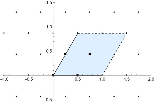
Figure 1: The 4-point $A_{2}$-universally optimal configuration $\omega^{*}_{4}$.

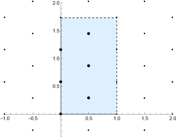
Figure 2: The 6-point $A_{2}$-universally optimal configuration $\omega^{*}_{6}$.

We can rephrase Theorem 1 in terms of the energies of infinite configurations, for which we follow the notation of [10]. Let $B(x,r)$ be the ball of radius $r>0$ centered at $x$. If $C$ is an infinite, multiset in $\mathbb{R}^{d}$ such that every ball intersects finitely many points, we call it an infinite configuration. Define $C_{r}:C\cap B(0,r)$ and the density of $C$ as

$$\lim_{r\rightarrow\infty}\frac{|C_{r}|}{{\rm Vol}(B(0,r))},$$

assuming the limit exists and is finite. Similarly to above, for a lower semi-continuous map $f:[0,\infty)\rightarrow[0,\infty]$ of $d$-rapid decay, we define the $f$-energy of an $n$-point configuration $\omega_{n}=\{x_{1},\dots,x_{n}\}\subseteq\mathbb{R}^{d}$ as

$$E_{f}(\omega_{n}):=\sum_{\begin{subarray}{c}1\leq i,j\leq n\\ i\neq j\end{subarray}}f(|x_{i}-x_{j}|^{2}).$$

and the infimum over all $n$-point configurations contained in some set $X$ as $\mathcal{E}_{f}(n,X)$, where we extend the definition to $n\not\in\mathbb{N}$ via linear interpolation. Configurations achieving this infimum are called $f$-optimal on $X$. Then for a configuration $C$ of density $\rho$, the lower $f$-energy of $C$ is

$$E^{l}_{f}(C):=\liminf_{r\rightarrow\infty}\frac{E_{f}(C_{r})}{|C_{r}|}.$$

If the limit exists, we’ll write it as $E_{f}(C)$ and call it the $f$-energy of $C$. A configuration $C^{\prime}$ of density $\rho$ is $f$-optimal if

$$E_{f}(C^{\prime})\leq E^{l}_{f}(C)$$

for every configuration $C$ of density $\rho$, and universally optimal if it is $f_{a}$-optimal for all $a>0$. Similarly, a configuration $C^{\prime}$ is universally optimal among $S$ if we further restrict $C$ to elements of $S$. We’ll also say an infinite configuration $C$ is an $N$-point $\Lambda$-periodic configuration if

$$C=\cup_{i=1}^{N}x_{i}+\Lambda$$

for some set of representatives $\omega_{N}^{C}=\{x_{1},\dots,x_{n}\}$. Then we have the following connection between the $f$-energy of $C$, and the $F_{f,\Lambda}$ energy of $\omega_{N}^{C}$ (cf. [8, Lemma 9.1] or [4, Chapter 10]).

Proposition 2.

Let $C$ be an $N$-point $\Lambda$-periodic configuration with $\omega_{N}^{C}$ a set of representatives, and $f:x^{2}\rightarrow e^{-ax^{2}}$ for some $a>0$. Then $E_{f}(C)$ exists and

$$E_{f}(C)=\frac{1}{N}\left(E_{F_{f,\Lambda}}(\omega_{N}^{C})+N\sum_{0\neq v\in\Lambda}f(v)\right).$$

Thus, Theorem 1 can be restated as follows: $A_{2}/2$ is universally optimal among all 4-point $A_{2}$-periodic configurations, and a rotation and scaling of $A_{2}$ is universally optimal among all 6-point $L$-periodic configurations.

As motivation for studying the above periodic energy problems arising from the $A_{2}$ lattice, we review in Section 2.7 a proof of the universal optimality of $\mathbb{Z}$, which proceeds through the analogous periodic approach. As far as the authors are aware, this proof is the simplest route to showing the universal optimality of $\mathbb{Z}$. The main difference between the $\mathbb{Z}$ and $A_{2}$ cases is the presence of a simple error formula for univariate hermite interpolation that is not available for general bivariate interpolation. As a result, the most difficult portions of our proof of Theorem 1 involve showing that our proposed interpolants stay below their potentials on the relevant domains.
Moreover, we find the small cardinality examples of the main theorem interesting regardless of whether the periodic energy approach leads to a proof of the universal optimality of $A_{2}$. Such optimality results can often be surprisingly difficult, even in the case of simple potentials with configurations restricted to nice spaces. For example, the case of proving optimality for the Riesz potentials among configurations on $S^{2}$ is notoriously difficult even for 5 points (recently rigorously handled with computer-assisted calculations in [32]) and remains open for $n\not\in\{2,3,4,5,6,12\}$.

2 Lattices and Linear Programming Bounds for Periodic Energy

2.1 Preliminaries: Lattices and Fourier Series

We first gather some basic definitions and properties of lattices in $\mathbb{R}^{d}$.

Definition 2.1.

Let $\Lambda\subset\mathbb{R}^{d}$.

• $\Lambda$ is a lattice in $\mathbb{R}^{d}$ if $\Lambda:=V\mathbb{Z}^{d}=\left\{\sum_{i=1}^{d}a_{i}v_{i}\mid a_{1},a_{2},\ldots,a_{d}\in\mathbb{Z}\right\}$ for some nonsingular $d\times d$ matrix $V$ with columns $v_{1},\ldots v_{d}$. We refer to $V$ as a generator for $\Lambda$.

• Once a choice of generator $V$ is specified, we let $\Omega_{\Lambda}:=V\mathbb{[}0,1)^{d}$ denote the parallelepiped fundamental domain for $\Lambda$. The co-volume of $\Lambda$ defined by $\left|\Lambda\right|:=|\det V|$ is the volume of $\Omega_{\Lambda}$ which is, in fact, the same for any Lebesgue measurable fundamental domain for $\mathbb{R}^{d}/\Lambda$ where $\Lambda$ acts on $\mathbb{R}^{d}$ by translation.

• The dual lattice $\Lambda^{*}$ of a lattice $\Lambda$ with generator $V$ is the lattice generated by $V^{-T}=(V^{T})^{-1}$ or, equivalently, $\Lambda^{*}:=\{v\in\mathbb{R}^{d}\mid w\cdot v\in\mathbb{Z}\text{ for all }w\in\Lambda\}.$

• We denote by $S_{\Lambda}$ the symmetry group of $\Lambda$ consisting of isometries on $\mathbb{R}^{d}$ fixing $\Lambda$ and denote by $G_{\Lambda}$ the subgroup of $S_{\Lambda}$ fixing the origin (and thus can be considered as elements of the orthogonal group $O(d)$). Note that $G_{\Lambda}=S_{\Lambda}/\Lambda$ where we identify $v\in\Lambda$ with the translation $\cdot+v$. Further, note that $G_{\Lambda^{*}}=G_{\Lambda}$ since elements of $O(d)$ preserve inner products.

Let $\Lambda$ be a lattice in $\mathbb{R}^{d}$ with generator $V$ and fundamental domain $\Omega_{\Lambda}$. We let $L^{2}(\Omega_{\Lambda})$ denote the Hilbert space of complex-valued $\Lambda$-periodic functions on $\mathbb{R}^{d}$ with inner product $\langle f,g\rangle=\int_{\Omega_{\Lambda}}f(x)\overline{g(x)}\,dx$. Then $\{e^{2\pi iv\cdot x}\mid v\in\Lambda^{*}\}$ forms an orthogonal basis of $L^{2}(\Omega_{\Lambda})$ yielding the Fourier expansion of a function $g\in L^{2}(\Omega_{\Lambda})$:

$$g(x)=\sum_{v\in\Lambda^{*}}\hat{g}_{v}e^{2\pi iv\cdot x}$$ (4)

with Fourier coefficients $\hat{g}_{v}:=\frac{1}{|\Lambda|}\int_{\Omega_{\Lambda}}g(x)$ for $v\in\Lambda^{*}$ where equality (and the implied unconditional limit on the right hand side) holds in $L^{2}(\Omega_{\Lambda})$. Of course, elements of $L^{2}(\Omega_{\Lambda})$ are actually equivalence classes of functions. If $g\in L^{2}(\Omega_{\Lambda})$ contains an element of $C(\mathbb{R}^{d})$, then we identify $g$ with its continuous representative and write $g\in L^{2}(\Omega_{\Lambda})\cap C(\mathbb{R}^{d})$. As will be the case in our applications, if $g\in L^{2}(\Omega_{\Lambda})$ is such that $\sum_{v\in\Lambda^{*}}|\hat{g}_{v}|<\infty$, then the right-hand side of (4) converges uniformly and unconditionally to $g$ and so $g\in L^{2}(\Omega_{\Lambda})\cap C(\mathbb{R}^{d})$ and (4) holds pointwise for every $x\in\mathbb{R}^{d}$.

We say that $g\in L^{2}(\Omega_{\Lambda})$ is conditionally positive semi-definite (CPSD) if the Fourier coefficients $\hat{g}_{v}\geq 0$ for all $v\in\Lambda^{*}\setminus\{0\}$ and $\sum_{v\in\Lambda^{*}}\hat{g}_{v}<\infty$ and say that a CPSD $g$ is positive semi-definite (PSD) if $\hat{g}_{0}\geq 0$. Note that the product of two PSD functions in $L^{2}(\Omega_{\Lambda})$ is PSD.

2.2 Lattice symmetry, symmetrized basis functions, and polynomial structure

Let $\Lambda$ be a lattice in $\mathbb{R}^{d}$, $f:[0,\infty)\to[0,\infty]$ have $d$-rapid decay, and $\sigma\in G_{\Lambda}$. Since $\sigma^{-1}\in G_{\Lambda}$ and $\sigma$ is an isometry, we have

$$F_{f,\Lambda}(\sigma x)=\sum_{v\in\sigma^{-1}\Lambda}f(\lvert\sigma x+\sigma v\rvert^{2})=\sum_{v\in\Lambda}f(\lvert x+v\rvert^{2})=F_{f,\Lambda}(x).$$

Then $F_{f,\Lambda}$ is also $\Lambda$-periodic and we obtain:

Proposition 3.

Suppose $f:[0,\infty)\to[0,\infty]$ has $d$-rapid decay and $\Lambda$ is a lattice in $\mathbb{R}^{d}$. Then for all $\sigma\in G_{\Lambda}$, $v\in\Lambda$ and $x\in\mathbb{R}^{2}$, we have $F_{f,\Lambda}(\sigma x+v)=F_{f,\Lambda}(x)$ showing that $F_{f,\Lambda}$ is $S_{\Lambda}$-invariant.

We next recall that $g\in L^{2}(\Omega_{\Lambda})$ is $\sigma$-invariant for $\sigma\in G_{\Lambda}$ if and only if the Fourier coefficients of $g$ are $\sigma$-invariant, as described in the next proposition.

Proposition 4.

Suppose $g\in L^{2}(\Omega_{\Lambda})$ and $\sigma\in G_{\Lambda}$. Then $g(\sigma x)=g(x)$ for a.e. $x\in\mathbb{R}^{d}$ if and only if $\hat{g}_{\sigma v}=\hat{g}_{v}$ for all $v\in\Lambda^{*}$.

Proof.

Since $\sigma^{-1}\in G_{\Lambda^{*}}=G_{\Lambda}$, we have

$$g(\sigma x)=\sum_{v\in\Lambda^{*}}\hat{g}_{v}e^{2\pi iv\cdot(\sigma x)}=\sum_{v\in\sigma^{-1}\Lambda^{*}}\hat{g}_{v}e^{2\pi i(\sigma v)\cdot(\sigma x)}=\sum_{v\in\Lambda^{*}}\hat{g}_{\sigma v}e^{2\pi iv\cdot x}.$$

The proposition then follows from uniqueness properties of the Fourier expansion. ∎

Let $\Gamma$ be a subgroup of $G_{\Lambda}$. For $v\in\Lambda^{*}$, let $C_{v}^{\Gamma}$ be the $\Lambda$-periodic function defined by

$$C_{v}^{\Gamma}(x):=\frac{1}{|\Gamma|}\sum_{\sigma\in\Gamma}e^{2\pi i(\sigma v)\cdot x}=\frac{1}{|\Gamma(v)|}\sum_{v^{\prime}\in\Gamma(v)}e^{2\pi iv^{\prime}\cdot x},\quad x\in\mathbb{R}^{d}.$$ (5)

where $\Gamma(v)$ denotes the orbit $\Gamma(v)=\{\sigma v\mid\sigma\in\Gamma\}.$ We write $C_{v}$ for $C_{v}^{\Gamma}$ when $\Gamma$ is unambiguous. If $g\in L^{2}(\Omega_{\Lambda})$ and $g$ is $G_{\Lambda}$-invariant (i.e., if $g(\sigma\cdot)=g$ for all $\sigma\in G_{\Lambda}$), then we may rewrite (4) as

$$g(x)=\sum_{v\in\Lambda^{*}/\Gamma}|\Gamma(v)|\,\hat{g}_{v}\,C_{v}^{\Gamma}(x).$$ (6)

We next consider the case of a rectangular lattice by which we mean a lattice of the form $\Lambda_{R}=(a_{1}\mathbb{Z})\times\cdots(a_{d}\mathbb{Z})$ with $a_{1},\ldots,a_{d}>0$. The symmetry group of a rectangular lattice in $\mathbb{R}^{d}$ contains the subgroup $H$ of order $2^{d}$ generated by the coordinate reflections

$$R_{j}(x_{1},\dots,x_{j},\ldots,x_{d})=(x_{1},\dots,-x_{j},\ldots,x_{d}),\qquad j=1,2,\ldots,d.$$ (7)

Let $v\in\Lambda^{*}=(1/a_{1})\mathbb{Z}\times\cdots(1/a_{d})\mathbb{Z}$, and note that $v=(k_{1}/a_{1},k_{2}/a_{2},\dots,k_{d}/a_{d})$ for some $k_{1},\dots,k_{d}\in\mathbb{Z}$. A straightforward induction on $d$ gives

$$C_{v}^{H}(x)=\prod_{i=1}^{d}\cos(2\pi k_{i}x_{i}/a_{i}))=\prod_{i=1}^{d}T_{|k_{i}|}(\cos(2\pi x_{i}/a_{i})).$$ (8)

Recall the $\ell$th Chebyshev polynomial of the first kind defined by $\cos(\ell\theta)=T_{\ell}(\cos\theta)$ for $\ell=0,1,2,\ldots$. We then have the following proposition.

Proposition 5.

Let $\Lambda_{R}=(a_{1}\mathbb{Z})\times\cdots(a_{d}\mathbb{Z})$ with $a_{1},\ldots,a_{d}>0$. If $v\in\Lambda_{R}^{*}$, then $v=(k_{1}/a_{1},k_{2}/a_{2},\dots,k_{d}/a_{d})$ for some $k_{1},\dots,k_{d}\in\mathbb{Z}$ and

$$C_{v}^{H}(x)=\prod_{i=1}^{d}T_{|k_{i}|}(t_{i}),$$ (9)

where $t_{i}=\cos(2\pi x_{i}/a_{i})\in[-1,1]$ for $i=1,2,\ldots,d$.

We next deduce a polynomial structure for $C_{v}^{\Lambda}$ for lattices $\Lambda$ that are invariant under the coordinate reflections $R_{j}$; i.e., such that $H\subseteq G_{\Lambda}$.

Proposition 6.

Let $\Lambda\subseteq\mathbb{R}^{d}$ be a lattice such that $H\subseteq G_{\Lambda}$. Then $\Lambda$ contains a rectangular lattice $\Lambda_{R}=(a_{1}\mathbb{Z})\times\cdots\times(a_{d}\mathbb{Z})$ and the function $C^{G_{\Lambda}}_{v}(x)$ is a polynomial in the variables $t_{j}=\cos(2\pi x_{j}/a_{j})$ for $j=1,2,\ldots,d$ and any $v\in\Lambda^{*}$.

Proof.

We first show that $\Lambda$ must contain some rectangular sublattice (i.e., of the form $\Lambda_{R}=(a_{1}\mathbb{Z})\times\cdots\times(a_{d}\mathbb{Z})$). Since $\Lambda$ is full-rank, for each $j=1,2,\ldots,d$, there is some $w^{j}\in\Lambda$ such that $a_{j}:=2w^{j}\cdot e^{j}\neq 0$ where $e^{j}$ denotes the $j$-th coordinate unit vector. Then $a_{j}e^{j}=w^{j}-R_{j}w^{j}\in\Lambda$, and so the rectangular lattice $(a_{1}\mathbb{Z})\times\cdots\times(a_{d}\mathbb{Z})$ is a sublattice of $\Lambda$.

Let $v\in\Lambda^{*}$. Since $\Lambda_{R}\subseteq\Lambda$, $\Lambda^{*}\subseteq\Lambda_{R}^{*}$, so $v\in\Lambda_{R}^{*}$. Let $C=\{\sigma_{1},\dots,\sigma_{[G_{\lambda}:H]}\}$ be a set of right coset representatives of $H$ in $G_{\Lambda}$, so that $|C||H|=|G|$. Then we have

$$\begin{split}C^{G_{\Lambda}}_{v}&=\frac{1}{|G_{\Lambda}|}\sum_{g\in G_{\Lambda}}e^{2\pi igv\cdot x}\\ &=\frac{1}{|C|}\sum_{\sigma\in C}\frac{1}{|H|}\sum_{h\in H}e^{2\pi ih\sigma v\cdot x}\\ &=\frac{1}{|C|}\sum_{\sigma\in C}C^{H}_{\sigma v}.\end{split}$$ (10)

Proposition 5 implies $C^{H}_{\sigma v}$ is polynomial in the variables $t_{j}=\cos(2\pi x_{j}/a_{j})$ and thus so is $C^{G_{\Lambda}}_{v}$. ∎

With $\Lambda$ and $\Lambda_{R}$ as in Proposition 6, we consider the change of variables

$$t_{i}:=\cos(2\pi x_{i}/a_{i}),\qquad i=1,...,d.$$ (11)

We then let $T_{a_{1},...,a_{d}}:\mathbb{R}^{d}\rightarrow\mathbb{R}^{d}$ be defined by

$$T_{a_{1},\dots,a_{d}}(x_{1},...,x_{d}):=(t_{1},\dots,t_{d}).$$ (12)

For any $\Lambda_{R}$-periodic function $h$ with $H$-symmetry, $\tilde{h}$ will refer to the function defined on $[-1,1]^{d}$ by

$$\tilde{h}(t)=h\left(\frac{a_{1}\arccos t_{1}}{2\pi},\dots,\frac{a_{d}\arccos t_{2}}{2\pi}\right),$$

which ensures $\tilde{h}(t)=h(x)$. We say that $\tilde{h}$ is (C)PSD if $h$ is (C)PSD.

It follows by Proposition 6 that the maps

$$P^{\Phi}_{v}:=\tilde{C}^{G_{\Phi}}_{v},\qquad v\in\Phi^{*},$$ (13)

are polynomials in the variables $t_{1},\dots,t_{d}$. It then follows that the collection of polynomials $\{P_{v}^{\Phi}\mid v\in\Phi^{*}/G_{\Phi}\}$ is orthogonal with respect to the measure $(1-t_{1}^{2})^{-1/2}\cdots(1-t_{d}^{2})^{-1/2}dt_{1}\,\cdots\,dt_{d}$ on $[-1,1]^{d}$. Furthermore, $\tilde{h}$ is CPSD if and only if its expansion in terms of these polynomials has coefficients that are non-negative and summable.

We shall also write $P_{v}$ when the choice of $\Phi$ is clear. Similarly, the $T_{a_{1},\dots,a_{d}}$ image of any subset $D\subseteq[0,1/2]\times[0,\sqrt{3}/2]$ will be denoted $\tilde{D}$. In any case where we do so, the choice of rectangular lattice (and hence the choice of $a_{i}$’s will be clear).

2.3 Linear Programming Bounds for Periodic Energy

If $g\in L^{2}(\Omega_{\Lambda})$ is CPSD and $\omega_{n}$ is an arbitrary $n$-point configuration in $\mathbb{R}^{d}$, then the following fundamental lower bound holds:

$$\begin{split}E_{g}(\omega_{n})&=\sum_{x\neq y\in\omega_{n}}g(x-y)=-ng(0)+\sum_{x,y\in\omega_{n}}g(x-y)\\ &=-ng(0)+\sum_{v\in\Lambda^{*}}\hat{g}_{v}\sum_{x,y\in\omega_{n}}e^{2\pi iv\cdot x}e^{-2\pi iv\cdot y}\\ &=-ng(0)+\sum_{v\in\Lambda^{*}}\hat{g}_{v}\left\lvert\sum_{x\in\omega_{n}}e^{2\pi iv\cdot x}\right\rvert^{2}\\ &\geq n^{2}\hat{g}_{0}-ng(0).\end{split}$$ (14)

For $v\in\mathbb{R}^{d}$ we refer to

$$M_{v}(\omega_{n}):=\sum_{x\in\omega_{n}}e^{2\pi iv\cdot x},$$

as the $v$-moment of $\omega_{n}$. Note that equality holds in (14) if and only if

$$\hat{g}_{v}M_{v}(\omega_{n})=0,\qquad v\in\Lambda^{*}\setminus\{0\}.$$ (15)

The next proposition follows immediately from (14) and the condition (15) for equality in (14). The calculations in (14) are similar to the proof of the linear programming bounds for energy found in [8, Proposition 9.3] and is closely related to Delsarte-Yudin energy bounds for spherical codes (cf. [4, Chapters 5.5 and 10.4]).

Proposition 7.

Let $F:\mathbb{R}^{d}\to[0,\infty]$ be $\Lambda$-periodic, and suppose $g\in L^{2}(\Omega_{\Lambda})$ is CPSD such that $g\leq F$. Then for any $n$-point configuration $\omega_{n}$, we have

$$E_{F}(\omega_{n})\geq E_{g}(\omega_{n})\geq n^{2}\hat{g}_{0}-ng(0)$$ (16)

with equality holding throughout (16) if and only if the following two conditions hold:

1. $g(x-y)=F(x-y)$ for all $x\neq y\in\omega_{n}$,

2. $\hat{g}_{v}M_{v}(\omega_{n})=0$, for all $v\in\Lambda^{*}\setminus\{0\}$.

If (a) and (b) hold, then $E_{F}(\omega_{n})=\mathcal{E}_{F}(n)$.

Remark.

If $F:\mathbb{R}^{d}\to[0,\infty]$ is $\Lambda$-periodic and $G_{\Lambda}$-invariant and $g\in L^{2}(\Omega_{\Lambda})$ is CPSD such that $g\leq F$, then the $S_{\Lambda}$-invariant function

$$g^{\rm sym}(x):=\frac{1}{|G_{\Lambda}|}\sum_{\sigma\in G_{\Lambda}}g((\sigma v)\cdot x),\qquad x\in\mathbb{R}^{d}$$

is also CPSD and satisfies $g^{\rm sym}\leq F$. Thus, we may restrict our search for functions $g$ to use in Proposition 7 to those of the form given in (6) in which case we only need verify the condition that $g\leq F$ on the fundamental domain of the action of $S_{\Lambda}$ on $\mathbb{R}^{d}$. In particular, when $\Lambda=A_{2}$, we have the representative set

$$\Delta_{A_{2}}:=\{(x_{1},x_{2})\mid 0\leq x_{1}\leq\frac{1}{2},0\leq x_{2}\leq x_{1}/\sqrt{3}\}$$

and when $\Lambda=L$, we’ll consider the representative set $[0,1/2]\times[0,\sqrt{3}/2]$.

2.4 Moments for certain lattice configurations

We consider moments of configurations obtained by restricting scalings of a lattice $\Lambda$ to the fundamental domain of a sublattice $\Phi$.

Theorem 8.

Suppose $\Phi$ is a sublattice of a lattice $\Lambda$ in $\mathbb{R}^{d}$. Let $\omega_{\Phi}:=\Lambda\cap\Omega_{\Phi}$ and $\kappa:=|\omega_{\Phi}|$ denote the index of $\Phi$ in $\Lambda$. For $m\in\mathbb{N}$, let

$$\mu_{\kappa m^{d}}:=(\frac{1}{m}\Lambda)\cap\Omega_{\Phi}.$$ (17)

Then for $v\in\Phi^{*}$, we have

$$M_{v}(\mu_{\kappa m^{d}})=\begin{cases}\kappa m^{d},&v\in m\Lambda^{*},\\ 0,&\text{otherwise.}\end{cases}$$ (18)

Furthermore, if $G_{\Phi}\subset G_{\Lambda}$, then for any $v\in\Phi^{*}$ and $\sigma\in G_{\Phi}$, we have $M_{\sigma v}(\mu_{\kappa m^{d}})=M_{v}(\mu_{\kappa m^{d}})$.

Proof.

Let $\Lambda=V\mathbb{Z}^{d}$; i.e., $V$ is a generator for $\Lambda$. Since $\Phi$ is a sublattice of $\Lambda$, there is some integer $d\times d$ matrix $W$ such that $VW$ is a generator for $\Phi$. Then $W$ is an that can be written in Smith Normal Form as $W=SDT$ where $S$ and $T$ are integer matrices with determinant $\pm 1$ (equivalently, their inverses are also integer matrices) and $D$ is a diagonal matrix with positive integer diagonal entries $\lambda_{1},\ldots,\lambda_{d}$. Then $\widetilde{V}=VS$ is a generator for $\Lambda$ and $U=\widetilde{V}D$ is a generator for $\Phi$. Choosing the fundamental domains $\Omega_{\Lambda}=\widetilde{V}[0,1)^{d}$ and $\Omega_{\Phi}=U[0,1)^{d}$ we may write

$$\mu_{\kappa m^{d}}=\{\frac{1}{m}\widetilde{V}j\mid j\in I_{m\lambda_{1}}\times\cdots\times I_{m\lambda_{d}}\},$$

where $I_{p}:=\{0,1,2,\ldots,p-1\}$. Let $v\in\Phi^{*}$ so that $v=U^{-T}k={\widetilde{V}}^{-T}D^{-1}k$ for some $k=(k_{1},k_{2},\dots,k_{d})\in\mathbb{Z}^{d}.$ Then $v\cdot(\frac{1}{m}\widetilde{V}j)=\frac{1}{m}j\cdot(D^{-1}k)$ and so

$$M_{v}(\mu_{\kappa m^{d}}) =\sum_{j\in I_{m\lambda_{1}}\times\cdots\times I_{m\lambda_{d}}}e^{2\pi i\frac{1}{m}j\cdot D^{-1}k}=\prod_{\ell=1}^{d}\left(\sum_{j_{\ell}=0}^{m\lambda_{\ell}-1}e^{2\pi i\frac{j_{\ell}k_{\ell}}{m\lambda_{\ell}}}\right)$$

$$=\begin{cases}m^{d}\lambda_{1}\cdots\lambda_{d},&k\in mD\mathbb{Z}^{d},\\ 0,&\text{otherwise},\end{cases}$$

where we used the finite geometric sum formula in the last equality. Noting that $\kappa=\lambda_{1}\cdots\lambda_{d}$ and that $v\in m\Lambda^{*}$ if and only if $k\in mD\mathbb{Z}^{d}$ establishes (18).

Finally, if $\sigma\in G_{\Phi}$ and $G_{\Phi}\subset G_{\Lambda}$, then $\sigma v\in m\Lambda^{*}$ if and only if $v\in m\Lambda^{*}$ which completes the proof. ∎

We define the index of a configuration $\omega_{n}\subset\mathbb{R}^{d}$ with respect to a lattice $\Phi\subset\mathbb{R}^{d}$ by

$$\mathcal{I}_{\Phi}(\omega_{n})=\{v\in\Phi^{*}\mid M_{v}(\omega_{n})=0\}.$$ (19)

It then follows from Theorem 8 that $\mathcal{I}_{\Phi}(\mu_{\kappa m^{d}})=\Phi^{*}\setminus(m\Lambda^{*})$.

2.5 Lattice theta functions

For $c>0$, the classical Jacobi theta function of the third type, is defined by

$$\theta(c;x):=\sum^{\infty}_{k=-\infty}e^{-\pi k^{2}c}e^{2\pi ikx},\qquad x\in\mathbb{R}.$$ (20)

Via Poisson Summation on the integers, we have

$$\theta(c;x)=c^{-1/2}\sum^{\infty}_{k=-\infty}e^{-\frac{\pi(k+x)^{2}}{c}},$$ (21)

and so, in terms of our earlier language for periodizing gaussians by lattices,

$$F_{a,\mathbb{Z}}(x)=(a/\pi)^{1/2}\theta(\frac{\pi}{a};x).$$ (22)

We’ll also use

$$\tilde{\theta}(c;t):=\theta\left(c,\frac{\arccos t}{2\pi}\right),\quad t\in[-1,1].$$

It follows from the symmetries of $\theta(c,x)$ that for all $x\in\mathbb{R}$,

$$\tilde{\theta}(c;\cos 2\pi x)=\theta(c;x),$$

and moreover, as shown below, $\tilde{\theta}$ is absolutely monotone on $[-1,1]$. First, we recall the Jacobi triple product formula.

Theorem 9.

Jacobi Triple Product Formula Let $z,q\in\mathbb{C}$ with $\lvert q\rvert<1$ and $z\neq 0$. Then

$$\prod^{\infty}_{r=1}(1-q^{2r})(1+q^{2r-1}z^{2})(1+q^{2r-1}z^{-2})=\sum^{\infty}_{k=-\infty}q^{k^{2}}z^{2k}.$$

Applying the Jacobi triple product with $q=e^{-\pi c}$ and $z=e^{\pi ix}$, gives

$$\tilde{\theta}(c;t)=\prod^{\infty}_{r=1}(1-e^{-2\pi rc})(1+2e^{-2\pi rc}t+e^{-2(2r-1)\pi c}).$$ (23)

It’s elementary to verify that $\tilde{\theta}(c;\cdot)$ is entire, and that we may compute derivatives by applications of the product rule to (23). Hence, we arrive at the following proposition:

Proposition 10.

For any $c>0$, the function $\tilde{\theta}=\tilde{\theta}(c;\cdot):[-1,1]\rightarrow(0,\infty)$ is strictly absolutely monotone on $[-1,1]$ and its logarithmic derivative $\tilde{\theta}^{\prime}/\tilde{\theta}$ is strictly completely monotone on $[-1,1]$.

If $\Lambda_{R}=(a_{1}\mathbb{Z})\times\cdots\times(a_{d}\mathbb{Z})$ is a rectangular lattice, then $F_{a,\Lambda_{R}}(x)$ is a tensor product of such functions:

$$\begin{split}F_{a,\Phi}(x)&=\sum_{v\in\Phi}e^{-a\|x+v\|^{2}}=\sum_{k\in\mathbb{Z}^{d}}\prod_{i=1}^{d}e^{-aa_{i}^{2}(x_{i}/a_{i}+k_{i})^{2}}\\ &=\prod_{i=1}^{d}\left(\sum_{k_{i}\in\mathbb{Z}}e^{-aa_{i}^{2}(\frac{x_{i}}{a_{i}}+k_{i})^{2}}\right)=\prod_{i=1}^{d}F_{aa_{i}^{2},\mathbb{Z}}(x_{i}/a_{i}).\end{split}$$ (24)

If $\Lambda$ contains a rectangular sublattice $\Lambda_{R}$, then we may write $F_{\Lambda}$ as a sum of such tensor products.

Proposition 11.

Suppose $\Lambda$ is a lattice in $\mathbb{R}^{d}$ that contains a rectangular sublattice $\Lambda_{R}=(a_{1}\mathbb{Z})\times\cdots\times(a_{d}\mathbb{Z})$ and let $\omega_{\Phi}=\Lambda\cap\Omega_{\Lambda_{R}}$. Then

$$F_{a,\Lambda}(x)=\sum_{y\in\omega_{\Lambda_{R}}}F_{a,\Lambda_{R}}(x+y).$$ (25)

Proof.

The formula follows immediately from $\Lambda=\omega_{\Phi}+\Phi$. ∎

2.6 Polynomial interpolation and linear programming bounds for lattice configurations

Combining the previous results in this section, we obtain the following general polynomial interpolation framework for linear programming bounds. For convenience, we shall write

$$W_{\Phi}:=\Phi^{*}/G_{\Phi}\text{ and }\Delta_{\Phi}:=\mathbb{R}^{d}/S_{\Phi},$$ (26)

to denote some choice of the respective fundamental domains for a lattice $\Phi\subset\mathbb{R}^{d}$.

Theorem 12.

Let $\Phi\subset\mathbb{R}^{d}$ be such that $H\subseteq G_{\Phi}$ where $H$ is the coordinate symmetry group (see Sec. 2.2) and suppose $F:\mathbb{R}^{d}\to(-\infty,\infty]$ is $S_{\Phi}$ invariant. By Proposition 6, $\Phi$ contains a rectangular sublattice

$$a_{1}\mathbb{Z}\times\cdots\times a_{d}\mathbb{Z},$$

which induces the change of variables $T:=T_{a_{1},\ldots,a_{d}}$ defined in (12) and associated polynomials $P^{\Phi}_{v}$ defined in (13). Suppose $(c_{v})_{v\in W_{\Phi}}$ is such that (a) $c_{v}\geq 0$, for all nonzero $v\in W_{\Phi}$ , (b) $\sum_{v\in W_{\Phi}}c_{v}<\infty$, and (c) the continuous function

$$\tilde{g}:=c_{0}+\sum_{v\in W_{\Phi}}c_{v}P^{G_{\Phi}}_{v}.$$

satisfies $\tilde{g}\leq\tilde{F}$ on $\tilde{\Delta}_{\Phi}$.

Then for any $n$-point configuration $\omega_{n}=\{x_{1},\ldots,x_{n}\}\subset\mathbb{R}^{d}$, we have

$$E_{F}(\omega_{n})\geq E_{g}(\omega_{n})=n^{2}c_{0}-n\tilde{g}_{(}1,\ldots,1),$$ (27)

where equality holds if and only if

1. $\tilde{g}(t)=\tilde{F}(t)$ for all $t\in T(\{x_{i}-x_{j}\mid i\neq j\in\{1,\ldots,n\}\})$ and

2. $c_{v}M_{\sigma v}(\omega_{n})=0$ for all $v\in W_{\Phi}$ and $\sigma\in G_{\Phi}$.

We now consider sufficient conditions for the $F$-optimality of configurations of the form $\mu_{\kappa m^{d}}=\frac{1}{m}\Lambda\cap\Omega_{\Phi}$ as in (17). For such a configuration (when the choices of $\Lambda,\Phi,$ and $\Delta_{\Phi}$ are clear), we define

$$\tau_{\kappa m^{d}}:=(\frac{1}{m}\Lambda)\cap\Delta_{\Phi},$$ (28)

which equals $\mu_{\kappa m^{d}}\cap\Delta_{\Phi}$ if we choose $\Delta_{\Phi}\subset\Omega_{\Phi}.$

Corollary 13.

Suppose $\Phi$, $T:=T_{a_{1},\ldots,a_{d}}$, $\tilde{g}$, and $F$ are as in Theorem 12 and that $\Phi\subseteq\Lambda$, and $G_{\Phi}\subseteq G_{\Lambda}$ for some lattice $\Lambda\subset\mathbb{R}^{d}$. Then the configuration $\mu_{\kappa m^{d}}=\frac{1}{m}\Lambda\cap\Omega_{\Phi}$ defined in Prop. 8 is $F$-optimal if

1. $c_{v}=0$ for all $v\in\left(m\Lambda^{*}\right)\cap W_{\Phi}$, and

2. $\tilde{g}(t)=\tilde{F}(t)$ for all $t\in\tilde{\tau}_{\kappa m^{d}}\setminus\{\mathbf{1}\}$ where $\mathbf{1}=(1,1,\ldots,1)\in\mathbb{R}^{d}$.

If such a $\tilde{g}$ exists, we refer to it as a ‘magic’ interpolant.

2.7 Example: Universal optimality of $\mathbb{Z}$

In this section we review an alternate proof of the universal optimality of $\mathbb{Z}$ that proceeds through the periodic approach. The main tool used here is the observation in Proposition 10 that the functions $\tilde{\theta}(c;t)$ are absolutely monotone. This proof is essentially from [33], but H. Cohn and A. Kumar were also aware of this approach [9]. The proof we give that equally spaced points are universally optimal on the unit interval is equivalent to that of [8] showing that the roots of unity are universally optimal on the unit circle.

Let $\omega^{\mathbb{Z}}_{m}=\{j/m\mid j=0,1,\ldots,m-1\}=\omega(\mathbb{Z},\mathbb{Z},m)$ and $t=\cos(2\pi x)$. Then

• $P_{k}^{\mathbb{Z}}(t)=T_{k}(t)$ for $k=0,1,2,\ldots$

• $\mathcal{I}(\omega^{\mathbb{Z}}_{m})=\mathbb{Z}\setminus(m\mathbb{Z})$

• With $\ell:=\lceil m/2\rceil$, we have $\tilde{\tau}_{m}=\{\cos(2\pi j/m)\mid j=0,1,\ldots,\ell\}=\{t_{j}\mid j=0,1,\ldots,\ell\}$ where $t_{j}:=\cos(2\pi(\ell-j)/m)$.

Recall that the Chebyshev polynomials of the second kind are defined by the relation

$$U_{\ell}(\cos\theta)\sin\theta=\sin((\ell+1)\theta),\qquad\ell=0,1,2,\ldots$$

and form the family of monic orthogonal polynomials with respect to the measure $(1-t^{2})dt$ on $[-1,1]$. These polynomials can be related to Chebyshev polynomials of the first kind through the relations

$$U_{\ell}(t)=\begin{cases}2\sum_{j=0}^{k}T_{2j+1}&\ell=2k+1\\ 1+2\sum_{j=1}^{k}T_{2j}&\ell=2k,\end{cases}$$

showing that $U_{\ell}$ is PSD for $\ell=0,1,2,\ldots$. Note that the points $-1\leq t_{1}<\cdots<t_{k}<1$ are also the roots of $U_{m-1}$. It then follows using the Christoffel-Darboux formula that the partial products $\prod_{\ell=0}^{j-1}(t-t_{\ell})$ have expansions in $U_{0},U_{1},\ldots,U_{j}$ with positive coefficients for $j=1,\ldots,\ell$ (see [8, Prop 3.2] or [4, Thm A.5.9]). Hence, each such partial product is PSD as is any product of such partial products; in particular, with $T=\{t_{0},t_{0},t_{1},t_{1},\ldots,t_{\ell},t_{\ell}\}$ the partial products $p_{j}(T;t)$ defined in (79) are PSD for $j\leq m$.

By Proposition 10, the function $\tilde{F}_{a,\mathbb{Z}}$ is absolutely monotone on $[-1,1]$ and, since the divided differences of an absolutely monotone function are non-negative, it follows that the interpolant $H_{T}(\tilde{F}_{a,\mathbb{Z}})(t)$ defined in (78) is PSD. Finally, the error formula (81) shows that $H_{T}(\tilde{F}_{a,\mathbb{Z}})\leq\tilde{F}_{a,\mathbb{Z}}$ on [-1,1].

3 The Linear Programming Framework for the families $\omega_{m^{2}},\omega_{2m^{2}},\omega_{3m^{2}},$ and $\omega_{6m^{2}}$

We explicitly apply Corollary 13 to the four families of periodic problems described in the introduction to obtain bivariate polynomial interpolation problems whose solutions would verify the $A_{2}$-universal optimality of $\omega_{m^{2}}$ and $\omega_{3m^{2}}$, and the $L$-universal optimality of $\omega_{2m^{2}}$ and $\omega_{6m^{2}}$. Observe that our four families of point configurations are of the form $\mu_{\kappa m^{2}}$ with the following choices of lattices $\Phi\subseteq\Lambda$:

1. $\omega^{*}_{m^{2}}$: $\Phi=A_{2},\Lambda=A_{2}$

2. $\omega^{*}_{2m^{2}}$: $\Phi=L,\Lambda=A_{2}$

3. $\omega^{*}_{3m^{2}}$: $\Phi=A_{2},\Lambda=\frac{1}{\sqrt{3}}A_{2}^{\pi/6}$

4. $\omega^{*}_{6m^{2}}$: $\Phi=L,\Lambda=\frac{1}{\sqrt{3}}A_{2}^{\pi/6}$.

It is straightforward to check that in all cases, $\Phi$ and $\Lambda$ satisfy the conditions of Theorem 12. Since both choices of $\Phi$, $A_{2}$ and $L$, contain $L$ as a rectangular sublattice, we will work with the following change of variables to induce our polynomial structure, as described in Proposition 6:

$$(t_{1},t_{2}):=\left(\cos(2\pi x_{1}),\cos\left(\frac{2\pi x_{2}}{\sqrt{3}}\right)\right).$$ (29)

We will use $T$ to denote the change of variables $T(x)=(t_{1}(x_{1}),t_{2}(x_{2}))$.

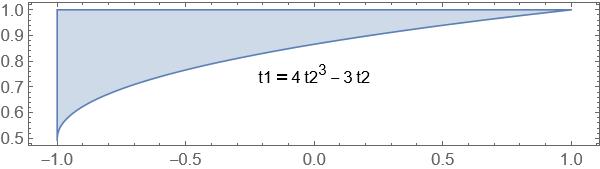
Figure 3: The region $\tilde{\Delta}_{A_{2}}$, pictured above, is our region of interpolation for the families $\omega^{*}_{m^{2}}$ and $\omega^{*}_{3m^{2}}$ (see sec. 3.4).

Importantly, the maps $F_{a,\Phi}$ are also well-behaved under this change of variables, as seen through decomposing $F_{a,\Phi}$ into $\theta$ functions as described in Proposition 11.

When $\Phi=L$, we obtain

$$F_{a,L}(x)=\frac{\pi}{\sqrt{3}a}\theta(\frac{\pi}{a};x_{1})\theta(\frac{\pi}{3a};\frac{x_{2}}{\sqrt{3}}).$$ (30)

As a result,

$$\tilde{F}_{a,L}(t_{1},t_{2}) :=F(\frac{\arccos(t_{1})}{2\pi},\frac{\sqrt{3}\arccos(t_{2})}{2\pi})$$

$$=\frac{\pi}{\sqrt{3}a}\theta(\frac{\pi}{a};\frac{\arccos(t_{1})}{2\pi})\theta(\frac{\pi}{3a};\frac{\arccos(t_{2})}{2\pi})$$

$$=\frac{\pi}{\sqrt{3}a}\tilde{\theta}(\frac{\pi}{a};t_{1})\tilde{\theta}(\frac{\pi}{3a};t_{2})$$

for $t_{1},t_{2}\in[-1,1]$. Thus, for fixed $t_{1}\in[-1,1]$, $\tilde{F}_{a,L}$ is strictly absolutely monotone as a function of $t_{2}$ and vice versa. We will use the absolute monotonicity in $t_{1}$ and $t_{2}$ repeatedly, and the simplicity of this formula for $\tilde{F}$ is one of the main motivations for considering the sublattice $L$.

On the other hand, when $\Phi=A_{2}$, we arrive at the following formula, which also appears in [1] and [33]:

$$F(x):=F_{a,A_{2}}(x)=\frac{\pi}{\sqrt{3}a}\left(\theta(\frac{\pi}{a};x_{1})\theta(\frac{\pi}{3a};\frac{x_{2}}{\sqrt{3}})+\theta(\frac{\pi}{3a};\frac{x_{2}}{\sqrt{3}}+\frac{1}{2})\theta(\frac{\pi}{a};x_{1}+\frac{1}{2})\right),$$ (31)

and

$$\begin{split}\tilde{F}(t)&:=F(\frac{\arccos t_{1}}{2\pi},\frac{\sqrt{3}\arccos t_{2}}{2\pi})\\ &=\frac{\pi}{\sqrt{3}a}(\tilde{\theta}(\frac{\pi}{a};t_{1})\tilde{\theta}(\frac{\pi}{3a};t_{2})+\tilde{\theta}(\frac{\pi}{a};-t_{1})\tilde{\theta}(\frac{\pi}{3a};-t_{2})).\end{split}$$ (32)

The next corollary follows immediately from the absolute monotonicity of $\tilde{\theta}$ (see Proposition 10).

Corollary 14.

For any nonnegative integers $l_{1}$ and $l_{2}$ whose sum $l_{1}+l_{2}$ is even, we have on all $[-1,1]^{2}$ that

$$\frac{\partial^{l_{1}+l_{2}}\tilde{F}}{\partial^{l_{1}}t_{1}\partial^{l_{2}}t_{2}}>0.$$

Finally, we’ll use the following lemma from [1] (also see [33]).

Lemma 15.

On all of $[-1,1]\times[\frac{1}{2},1]$, we have the inequalities

$$\frac{\partial\tilde{F}}{\partial t_{1}}>0,\frac{\partial\tilde{F}}{\partial t_{2}}\geq 0$$ (33)

where the equality holds if and only if $t_{1}=-1$, $t_{2}=\frac{1}{2}$. In particular, these inequalities hold on all $\tilde{\Delta}_{A_{2}}$.

Proof.

Since even partial deriviatives of $\tilde{F}$ are positive and every point $(t_{1},t_{2})\in\tilde{\Delta}_{A_{2}}$ satisfies $t_{1}\geq-1$ and $t_{2}\geq\frac{1}{2}$, it suffices to verify the inequalities

$$\frac{\partial\tilde{F}}{\partial t_{1}}(t_{1},t_{2})>0,\frac{\partial\tilde{F}}{\partial t_{2}}(t_{1},t_{2})\geq 0$$

at $(-1,\frac{1}{2})$. See [1] or [33]. ∎

As observed in [33] (also see [4, Chapter 10] and [16]), this Lemma 15 suffices to proves the $A_{2}$-universal optimality of the 2 and 3-point configurations discussed in the introduction (see section 3.5 for more detail).

We will make the following choices of fundamental domains $\mathbb{R}^{2}/S_{\Phi}$ and $\Phi^{*}/G_{\Phi}$. When $\Phi=L$, we take as a choice for $\Phi^{*}/G_{L}$ the set

$$W_{L}:=\left\{\begin{bmatrix}k_{1}\\ k_{2}/\sqrt{3}\end{bmatrix}\mid k_{1},k_{2}\in\mathbb{Z}\text{ and }k_{1},k_{2}\geq 0\right\}$$

and $[0,1/2]\times[0,\sqrt{3}/2]$ for $\mathbb{R}^{2}/S_{L}$. Likewise for $A_{2}$, we take the sets

$$W_{A_{2}}:=\left\{\begin{bmatrix}k_{1}\\ k_{2}/\sqrt{3}\end{bmatrix}\in L^{*}\mid 0\leq k_{2}\leq k_{1}\text{ and }k_{1}\equiv k_{2}\pmod{2}\,\right\}$$

and $\Delta_{A_{2}}$ (see Sec. 2.3) for $\Phi^{*}/G_{A_{2}}$ and $\mathbb{R}^{2}/S_{A_{2}}$, respectively.

Finally, the following characterizations of the dual lattices $\Lambda$ will be useful for determining which degree polynomials are available to us for interpolation. First, $L^{*}=\{[k_{1},k_{2}/\sqrt{3}]^{T}\mid k_{1},k_{2}\in\mathbb{Z}\}$. Then $A_{2}^{*}=\{v\in L^{*}\mid v\cdot e_{1}\equiv v\cdot\sqrt{3}e_{2}\pmod{2}\}$, and $\left(\frac{1}{\sqrt{3}}A_{2}^{\pi/6}\right)^{*}=\{v\in A_{2}^{*}\mid v\cdot\sqrt{3}e_{2}\equiv 0\pmod{3}\}$. Thus, using Theorem 8, the (non-redundant) sets of all $v$ for which $c_{v}$ may be non-zero in the construction of an interpolant $\tilde{g}_{a}$ are expressed by the index sets

$$\mathcal{I}_{m^{2}}:=\mathcal{I}_{A_{2}}(\omega_{m^{2}}^{*})\cap W_{A_{2}} =W_{A_{2}}/(mA_{2}^{*})$$ (34)

$$=\{[k_{1},k_{2}/\sqrt{3}]\mid k_{1},k_{2}\geq 0,k_{1}\equiv k_{2}\bmod 2,[k_{1},k_{2}]\neq m[j_{1},j_{2}]\}$$ (35)

$$\mathcal{I}_{2m^{2}}:=\mathcal{I}_{L}(\omega_{2m^{2}}^{*})\cap W_{L} =W_{L}/(mA_{2}^{*})$$ (36)

$$=\{[k_{1},k_{2}/\sqrt{3}]\mid k_{1},k_{2}\geq 0,[k_{1},k_{2}]\neq m[j_{1},j_{2}]\text{ for some }j_{1}\equiv j_{2}(\bmod 2)\}$$ (37)

$$\mathcal{I}_{3m^{2}}:=\mathcal{I}_{A_{2}}(\omega_{3m^{2}}^{*})\cap W_{A_{2}} =W_{A_{2}}/(mA_{2}^{*})$$ (38)

$$=\{[k_{1},k_{2}/\sqrt{3}]\mid k_{1},k_{2}\geq 0,k_{1}\equiv k_{2}\bmod 2,[k_{1},k_{2}]\neq m[j_{1},j_{2}]\text{ for some }j_{2}\equiv 0\bmod 3\}$$ (39)

$$\mathcal{I}_{6m^{2}}:=\mathcal{I}_{L}(\omega_{6m^{2}}^{*})\cap W_{L} =W_{L}/(mA_{2}^{*})$$ (40)

$$=\{[k_{1},k_{2}/\sqrt{3}]\mid k_{1},k_{2}\geq 0,[k_{1},k_{2}]\neq m[j_{1},j_{2}]\text{ for some }j_{1}\equiv j_{2}(\bmod 2),j_{2}\equiv 0\bmod 3\}.$$ (41)

3.1 The Polynomials $P^{L}_{v}$ and $P^{A_{2}}_{v}$

When $\Phi=L$, we have already shown that the functions are $P^{L}_{v}$ are tensors of Chebyshev Polynomials

$$P^{L}_{v}=T_{k_{1}}(t_{1})T_{k_{2}}(t_{2})$$

where $v=[k_{1},k_{2}/\sqrt{3}]^{T}$, $k_{1},k_{2}\geq 0$ is an arbitrary element of $W_{L}$. (see Proposition 5).
What can be said in the case when $\Phi=A_{2}$? These polynomials have been studied extensively (see [28], [29], and references therein). Of particular importance to $P^{A_{2}}_{v}$ are the polynomials $P_{v^{\prime}}$ and $P_{v^{\prime\prime}}$, where $v^{\prime}:=[1,1/\sqrt{3}]^{T}$ is the shortest non-zero vector in $W_{A_{2}}$ and $v^{\prime\prime}:=[2,0]^{T}$ is the next shortest vector. We have

$$P_{v^{\prime}} =\frac{1}{3}(-1+2t_{2}(t_{1}+t_{2})),$$ (42)

$$P_{v^{\prime\prime}} =\frac{1}{3}(-1+2t_{1}(t_{1}-3t_{2}+4t_{2}^{3})).$$ (43)

Perhaps surprisingly, every other $P_{v}$ can be expressed as a bivariate polynomial in $P_{v^{\prime}}$ and $P_{v^{\prime\prime}}$, i.e. for any $v\in A_{2}^{*}$, there exist coefficients $c_{i,j}$ (with only finitely many nonzero) such that

$$P_{v}=\sum_{i,j\geq 0}c_{i,j}(-1+2t_{2}(t_{1}+t_{2}))^{i}(-1+2t_{1}(t_{1}-3t_{2}+4t_{2}^{3}))^{j}$$

Note that since $P_{v^{\prime}}$ and $P_{v^{\prime\prime}}$ contain only monomials of even total degree, the same is true of arbitrary $P_{v}$. To further understand these bivariate polynomials, we set $\alpha=P_{v^{\prime}}$, $\beta=P_{v^{\prime\prime}}$ and introduce a notion of degree, first given in [31], on polynomials of the form $\alpha^{k_{0}}\beta^{k_{1}},i,j\geq 0$.

Definition 3.1.

The $A_{2}$-degree of $\alpha^{k_{0}}\beta^{k_{1}}$ is $2k_{0}+3k_{1}$.

If $v\in W_{A_{2}}$, then $v=k_{0}v^{\prime}+k_{1}v^{\prime\prime}$ for some unique $k_{0},k_{1}\geq 0$, and so we can likewise introduce the notion of the $A_{2}$ degree of $v\in W_{A_{2}}$ as $2k_{0}+3k_{1}$. We will denote the degree function as $\mathcal{D}$ for both polynomials and elements of $W_{A_{2}}$. Now we can introduce an ordering on $\{\alpha^{k_{0}}\beta^{k_{1}}:k_{0},k_{1}\geq 0\}$ by $A_{2}$-degree and break ties via the power of $\alpha$. Then the leading term (by $A_{2}$-degree) of $P_{v}$ is $\alpha^{k_{0}}\beta^{k_{1}}$. Certainly, this is true for our first polynomials, $P_{0}=1$, $P_{v^{\prime}}=\alpha$, and $P_{v^{\prime\prime}}=\beta$, and then an examination of the recursion generating the polynomials shows that the claim holds inductively (cf. [29]).

3.2 Interpolation Nodes

Our final step to applying Corollary 13 is to calculate the nodes $\tau_{\kappa m^{2}}$ for each family. Straight from the definition,

$$\tau_{\kappa m^{2}} =\omega_{\kappa m^{2}}\cap\Delta_{A_{2}},\hskip 28.45274pt\kappa=1,3$$ (44)

$$\tau_{\kappa m^{2}} =\omega_{\kappa m^{2}}\cap([0,1/2]\times[0,\sqrt{3}/2]),\hskip 28.45274pt\kappa=2,6$$ (45)

and so under the $T$ change of variables, we obtain

$$\tilde{\tau}_{m^{2}} =\left\{\left(\cos(\frac{\pi k_{1}}{m}),\cos(\frac{\pi k_{2}}{m})\right)\mid 0\leq 3k_{2}\leq k_{1}\leq m,k_{1}\equiv k_{2}(\bmod 2)\right\}$$ (46)

$$\tilde{\tau}_{2m^{2}} =\left\{\left(\cos(\frac{\pi k_{1}}{m}),\cos(\frac{\pi k_{2}}{m})\right)\mid 0\leq k_{1},k_{2}\leq m,k_{1}\equiv k_{2}(\bmod 2)\right\}$$ (47)

$$\tilde{\tau}_{3m^{2}} =\left\{\left(\cos(\frac{\pi k_{1}}{m}),\cos(\frac{\pi k_{2}}{3m})\right)\mid 0\leq k_{2}\leq k_{1}\leq m,k_{1}\equiv k_{2}(\bmod 2)\right\}$$ (48)

$$\tilde{\tau}_{6m^{2}} =\left\{\left(\cos(\frac{\pi k_{1}}{m}),\cos(\frac{\pi k_{2}}{3m})\right)\mid 0\leq 3k_{1},k_{2}\leq 3m,k_{1}\equiv k_{2}(\bmod 2)\right\}.$$ (49)

3.3 Interpolation Problem for $\omega_{m^{2}}$

With all the machinery now set up, we address the family $\omega_{m^{2}}^{*}$ and its base case, $\omega_{4}^{*}$. Recall $v^{\prime}:=[1,1/\sqrt{3}]$ is the shortest vector in $W_{A_{2}}$ and $P_{v^{\prime}}=\frac{1}{3}(-1+2t_{2}(t_{1}+t_{2}))$. In Section 4, we prove the $A_{2}$-universal optimality of $\omega_{4}^{*}$ by constructing for each $a>0$ a polynomial of the form $g_{a}(t_{1},t_{2}):=c_{0}+c_{1}P_{v^{\prime}}(t_{1},t_{2})$ with $c_{1}\geq 0$ such that $g_{a}\leq F_{a,A_{2}}$ on $\tilde{\Delta}_{A_{2}}$.

Figure 4: $\tilde{g}_{a}$ must stay below $\tilde{F}_{a}$ on $\tilde{\Delta}_{A_{2}}$ with equality at the corner point $(-1,1)$.

For general $m$, recalling the background on $G_{2}$ polynomials in Sec. 3.1, we note that

$$\{v\in W_{A_{2}}\mid\mathcal{D}(v)<2m\}\subset\mathcal{I}_{m^{2}}.$$

The containment holds because if $v=k_{0}v^{\prime}+k_{1}v^{\prime\prime}$ and $\mathcal{D}(v)<2m$, then $k_{0}<m$, and so $v\not\in mA_{2}^{*}$ (i.e. $v\in\mathcal{I}_{m^{2}}$). For the $m=2$ base case already discussed, our interpolant $\tilde{g}_{a}$ satisfies

$$\tilde{g}_{a}\in\text{span}\{P_{v}:v\in W_{A_{2}},\mathcal{D}(v)<2m\}.$$

3.4 Interpolation Problem for $\omega^{*}_{2m^{2}}$

Now to the case of $\omega^{*}_{2m^{2}}$ with base case $\omega^{*}_{2}$.

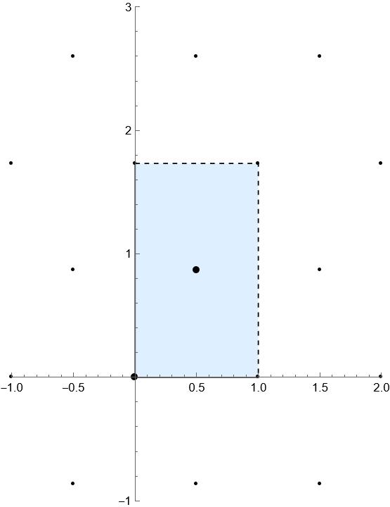
Figure 5: $\omega^{*}_{2}$, pictured above is $L$-universally optimal, and analogous results hold for any rectangular lattice.

The universal optimality of $\omega^{*}_{2}$ follows from

$$F_{a,L}(x)=\frac{\pi}{\sqrt{3}a}\theta(\frac{\pi}{a};x_{1})\theta(\frac{\pi}{3a};\frac{x_{2}}{\sqrt{3}}),$$

which takes its minimum at $(1/2,\sqrt{3}/2)$ for all $a$, as $\theta(c,x)$ takes its minimum at $x=1/2$ for all $c>0$ (see Proposition 10). Since the $F_{a,L}$ energy of a two-point configuration is determined only by the difference of the two points in the configuration, the universal optimality of $\omega^{*}_{2}$ immediately follows, and the same argument can be used to show for any rectangular lattice (cf. [16]) that a point at the origin and a point at the centroid of a rectangular fundamental domain yield a 2-point universally optimal configuration.

For the general case,

$$\{[k_{1},k_{2}/\sqrt{3}]^{T}:0\leq k_{1},k_{2}\text{ and }k_{1}+k_{2}<2m\}\subseteq\mathcal{I}_{2m^{2}},$$

and then

$$\text{span}\{P_{v}\mid v=[k_{1},k_{2}/\sqrt{3}]^{T}:0\leq k_{1},k_{2}\text{ and }k_{1}+k_{2}<2m\}=\mathcal{P}_{2m-1}(t_{1},t_{2}),$$

where $\mathcal{P}_{n}(t_{1},t_{2})$ is the set of bivariate polynomials of total degree at most $n$. For the first non-trivial case, $\omega^{*}_{8}$, we have numerical evidence that for each $a>0$, an interpolant $\tilde{g}_{a}$ exists in $P_{3}$ and satisfies the conditions of Corollary 13.

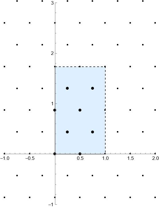
Figure 6: The 8 larger points comprise $\omega^{*}_{8}$

Figure 7: After applying the linear programming framework, it suffices to find for each $a>0$ an interpolant $\tilde{g}_{a}\in\mathcal{C}_{8}$ such that $\tilde{g}_{a}\leq\tilde{F}_{a}$ on $[-1,1]$ with equality at the 4 points shown.

3.5 Interpolation Problems for $\omega^{*}_{3m^{2}}$

Now to the case of $\omega^{*}_{3m^{2}}$ with base case $\omega^{*}_{3}$.

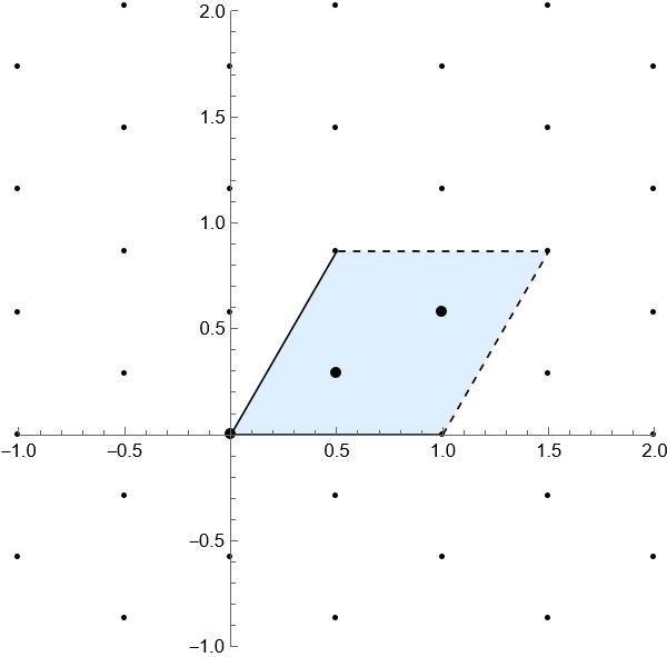
Figure 8: The 3 larger points comprise $\omega^{*}_{3}$

Figure 9: Almost the exact same analysis needed for the $A_{2}$-universal optimality of $\omega^{*}_{3}$ yields $A_{2}$-universal optimality of the two point honeycomb configuration

The universal optimality of $\omega^{*}_{3}$ (cf. [33] and [16]) follows from Lemma 15, which is used to show a global minimum of $F_{a,A_{2}}$ occurs at $(1/2,\sqrt{3}/6)$ for all $a>0$. This point, $(1/2,\sqrt{3}/6)$, is also the only difference $x-y$ (up to $S_{A_{2}}$ action) for $x,y\in\omega^{*}_{3}$. Thus for an arbitrary 3-point configuration $\omega_{3}$, we have

$$E_{F}(\omega_{3})\geq 6F(1/2,\sqrt{3}/6)=E_{F}(\omega^{*}_{3})$$

and so $\omega^{*}_{3}$ is $A_{2}$-universally optimal. This same line of argument is also used in [33] to show that the 2-point honeycomb configuration pictured above are $A_{2}$-universally optimal.

More generally, we suggest invoking $A_{2}$-degree as in the $m^{2}$ case to find a nice subset of $\mathcal{I}_{3m^{2}}$. We have the containment

$$\{v\in W_{A_{2}}\mid\mathcal{D}(v)<3m\}\subset\mathcal{I}_{3m^{2}}.$$

The containment holds because if $v=k_{0}v^{\prime}+k_{1}v^{\prime\prime}$ and $\mathcal{D}(v)<3m$, then either $v\not\in mA_{2}^{*}$ or $v=mv^{\prime}\not\in(\frac{1}{\sqrt{3}}A_{2}^{\pi/6})^{*}$.

3.6 Interpolation Problems for $\omega^{*}_{6m^{2}}$

It remains to consider the family $\omega_{6}^{*}$ and its base case $\omega_{6}^{*}$, whose universal optimality involves our most complex application of the linear programming bounds. In section 5, we prove the $L$-universal optimality of $\omega^{*}_{6}$ by constructing for each $a>0$ an interpolant of the form

$$g_{a}(t_{1},t_{2})=b_{0,0}+b_{1,0}t_{1}+b_{0,1}t_{2}+b_{1,1}t_{1}t_{2}+b_{0,2}t^{2}_{2}$$

where $b_{i,j}\geq 0$ for $(i,j)\neq 0$. In that section, we will explain in greater detail why such a $\tilde{g}_{a}$ satisfies the conditions of Corollary 13.

Figure 10: $\tilde{g}_{a}$ must stay below $\tilde{F}_{a}$ on $[-1,1]^{2}$ with equality at the three points shown

Finally, for arbitrary $m$, we propose a few nice subsets of $\mathcal{I}_{6m^{2}}$. First, we have the set

$$\{[k_{1},k_{2}/\sqrt{3}]^{T}:0\leq k_{1}<2m,0\leq k_{2}<3m\}\subseteq\mathcal{I}_{6m^{2}},$$

and

$$\text{span}\{P_{v}\mid v=[k_{1},k_{2}/\sqrt{3}]^{T}:0\leq k_{1}<2m,0\leq k_{2}<3m\}=\mathcal{P}_{2m-1}(t_{1})\times\mathcal{P}_{3m-1}(t_{2}).$$

Working with such a tensor space of polynomials is natural due to the tensor product nature of

$$\tilde{F}_{a,L}(x)=\frac{\pi}{\sqrt{3}a}\tilde{\theta}(\frac{\pi}{a};t_{1})\tilde{\theta}(\frac{\pi}{3a};t_{2}).$$

Notably, our interpolant, $\tilde{g}_{a}$, for $\omega^{*}_{6}$ satisfies $\tilde{g}_{a}\in\mathcal{P}_{1}(t_{1})\times\mathcal{P}_{2}(t_{2})$.

4 $A_{2}$-universal optimality of $\omega^{*}_{4}$

To prove $\omega^{*}_{4}$ is $A_{2}$-universally optimal, it remains to show for each $a>0$ that there are $c_{0},c_{1}\in\mathbb{R}$ with $c_{1}\geq 0$ such that the resulting interpolant $\tilde{g}_{a}(t_{1},t_{2}):=c_{0}+c_{1}P_{v^{\prime}}=c_{0}+c_{1}/3(-1+t_{2}(t_{1}+t_{2}))$ satisfies $\tilde{g}_{a}\leq\tilde{F}_{a}$ on $\tilde{\Delta}_{A_{2}}$ with equality at $(-1,1)$ or, equivalently, finding such an interpolant of the form

$$\ \tilde{g}_{a}(t_{1},t_{2}):=\tilde{F}_{a}(-1,1)+b_{1}t_{2}(t_{1}+t_{2})$$ (50)

for $b_{1}\geq 0$.
Our formulas for $\tilde{g}_{a}$ are defined piecewise in $a$. We set

$$b_{1}=\begin{cases}2\frac{\partial\tilde{F}}{\partial t_{1}}(-1,1/2)&\text{if }0<a\leq 21\\ \frac{\partial\tilde{F}}{\partial t_{2}}(-1,1)&\text{if }a>21.\end{cases}$$ (51)

Due to the different expansions used for $\theta$ (see (20) and (21)), we also find it convenient to rescale $\tilde{F}$ by a factor of $\sqrt{3}\pi/a$ for small $a$ case. Defining

$$\begin{split}\tilde{f_{1}}(t_{1})&:=\begin{cases}\tilde{\theta}(\frac{\pi}{a};t_{1}),&0<a\leq\pi^{2}\\ \sqrt{\frac{\pi}{a}}\tilde{\theta}(\frac{\pi}{a};t_{1})&a>\pi^{2},\end{cases}\\ \tilde{f_{2}}(t_{2})&:=\begin{cases}\tilde{\theta}(\frac{\pi}{3a};t_{2}),&0<a\leq\pi^{2}\\ \sqrt{\frac{\pi}{3a}}\tilde{\theta}(\frac{\pi}{3a};t_{2})&a>\pi^{2}.\end{cases}\end{split}$$ (52)

With this rescaling convention, it follows from (31) that

$$\tilde{F}(t_{1},t_{2})=\tilde{f_{1}}(t_{1})\tilde{f_{2}}(t_{2})+\tilde{f_{1}}(-t_{1})\tilde{f_{2}}(-t_{2}).$$ (53)

4.1 Constructing magic $\tilde{g}_{a}$

For all $a>0$, we will establish

Lemma 16.

For all points $(t_{1},t_{2})\in\tilde{\Delta}_{A_{2}}$, $\displaystyle\frac{\partial^{3}\tilde{F}}{\partial t_{1}\partial t_{2}^{2}}(t_{1},t_{2})>0.$

Proof.

Since even partial derivatives of $\tilde{F}$ are positive, it suffices to check the inequality at the minimal $t_{1}$ and $t_{2}$ values, when $t_{1}=-1$ and $t_{2}=\frac{1}{2}$. This check is handled in the appendix with large $a$ and small $a$ cases handled separately. ∎

Likewise, we have

Lemma 17.

Let $\tilde{h}$ be of the form $\tilde{F}(-1,1)+c_{1}t_{2}(t_{1}+t_{2})$ such that $\tilde{h}(-1,1/2)<\tilde{F}(-1,1/2)$ and $\frac{\partial\tilde{F}-\tilde{h}}{\partial t_{2}}(-1,1)\leq 0$. Then for all $t_{2}\in[1/2,1]$, $\tilde{F}(-1,t_{2})\geq\tilde{h}(-1,t_{2})$ with equality only when $t_{2}=1$.

Proof.

We abuse notation here and use $\tilde{F},\tilde{h}$ to refer to the one variable functions in $t_{2}$ obtained by fixing $t_{1}=-1$. By assumption on the form of $\tilde{h}$, Lemma 15, and the two assumed inequalities, we have $\tilde{F}(1/2)\geq\tilde{h}(1/2)$, $\tilde{F}^{\prime}(1/2)=\tilde{h}^{\prime}(1/2)=0$, $\tilde{F}(1)=\tilde{h}(1)$, and $\tilde{F}^{\prime}(1)\leq\tilde{h}^{\prime}(1)$. It follows that there are exists some point in $[1/2,1]$ at which $\tilde{F}^{\prime\prime}\leq\tilde{h}^{\prime\prime}$. Let $t_{2}^{\prime}\leq t_{2}^{\prime\prime}$ be such that $t_{2}^{\prime}$ and $t_{2}^{\prime\prime}$ respectively are the minimal and maximal points in $[1/2,1]$ at which $\tilde{F}^{\prime\prime}\leq\tilde{h}^{\prime\prime}$. For $t_{2}\geq t_{2}^{\prime\prime}$ we have $\tilde{F}^{\prime\prime}\geq\tilde{h}^{\prime\prime}$ with equality only at $t_{2}^{\prime\prime}$ since $(\tilde{F}-\tilde{h}){{}^{\prime\prime}}$ is strictly convex (recall $\tilde{F}^{(4)}>0$). Thus, we get $\tilde{F}\geq\tilde{h}$ by bounding $\tilde{F}-\tilde{h}$ below with a tangent line of $\tilde{F}-\tilde{h}$ at $1$ and equality holds only if $t_{2}=1$. Similarly, for $t_{2}\leq t_{2}^{\prime}$, we get the desired inequality with tangent approximation from $\frac{1}{2}$. For $t_{2}\in[t_{2}^{\prime},t_{2}^{\prime\prime}]$, we note that $\tilde{F}^{\prime\prime}=\tilde{h}^{\prime\prime}$ at the endpoints of the interval. Again using the strict convexity of $(\tilde{F}-\tilde{h}){{}^{\prime\prime}}$, we obtain $(\tilde{F}-\tilde{h})^{\prime\prime}\leq 0$ for the whole interval. Thus, $\tilde{F}(t_{2})\geq\tilde{h}(t_{2})$ by bounding the difference below with its secant line (since we’ve already established $\tilde{F}\geq\tilde{h}$ at the endpoints $t_{2}^{\prime},t_{2}^{\prime\prime}$), and equality can only hold at $t_{2}^{\prime\prime}$ if $t_{2}^{\prime\prime}=1$. ∎

4.1.1 Small $a$

Let $0<a\leq 21$. We will refer to $\tilde{g}_{a}$ as simply $\tilde{g}$. We’ll prove the following lemma in the appendix:

Lemma 18.

For $0<a\leq 21$, we have

$$\frac{\partial\tilde{F}}{\partial t_{2}}(-1,1),4(\tilde{F}(-1,1)-\tilde{F}(-1,1/2))\leq 2\frac{\partial\tilde{F}}{\partial t_{1}}(-1,1/2)\leq\frac{\partial^{2}(\tilde{F}-\tilde{g})}{\partial t_{1}\partial t_{2}}(-1,1/2).$$

We handle the proof piecewise, splitting into 2 cases, $0<a\leq\pi^{2}$ and $\pi^{2}<a\leq 21$ depending on which formulas we use for $\tilde{f_{1}}$ and $\tilde{f_{2}}$. These 3 inequalities suffice to show $\tilde{F}\leq\tilde{g}$. We certainly have $b_{1}>0$ since $b_{1}=2\frac{\partial\tilde{F}}{\partial t_{1}}(-1,1/2)>\frac{\partial\tilde{F}}{\partial t_{2}}(-1,1)>0$ where the first inequality holds by assumption and the next by Lemma 15. Next, we have

$$(\tilde{F}-\tilde{g})(-1,1/2)=\tilde{F}(-1,1/2)-\tilde{F}(-1,1)+\frac{1}{4}b_{1}>0$$

and likewise

$$\frac{\partial(\tilde{F}-\tilde{g})}{\partial t_{2}}(-1,1)=\frac{\partial\tilde{F}}{\partial t_{2}}(-1,1)-b_{1}<0.$$

Applying Lemma 17 and the previous two inequalities to $\tilde{g}$, we obtain $\tilde{F}\geq\tilde{g}$ for all points $(-1,t_{2})$ with $t_{2}\in[1/2,1]$ with equality only at $(-1,1)$, and since $\tilde{F}-\tilde{g}$ is convex in $t_{1}$, it remains to show that $\frac{\partial(\tilde{F}-\tilde{g})}{\partial t_{1}}\geq 0$ for all points of the form $(-1,t_{2})$, $t_{2}\in[1/2,1]$ (recall the picture of $\tilde{\Delta}_{A_{2}}$, Figure 4). By Lemma 16, $\frac{\partial(\tilde{F}-\tilde{g})}{\partial t_{1}}$ is convex in $t_{2}$ in $\tilde{\Delta}_{A_{2}}$, so we just need to show

$$\frac{\partial(\tilde{F}-\tilde{g})}{\partial t_{1}}(-1,1/2)\geq 0,\frac{\partial^{2}(\tilde{F}-\tilde{g})}{\partial t_{1}\partial t_{2}}(-1,1/2)\geq 0.$$

But these follow directly from our assumptions on $b_{1}$. Indeed,

$$\frac{\partial(\tilde{F}-\tilde{g})}{\partial t_{1}}(-1,1/2) =\frac{\partial\tilde{F}}{\partial t_{1}}(-1,1/2)-\frac{b_{1}}{2}=0$$ (54)

$$\frac{\partial^{2}(\tilde{F}-\tilde{g})}{\partial t_{1}\partial t_{2}}(-1,1/2) =\frac{\partial^{2}\tilde{F}}{\partial t_{1}\partial t_{2}}(-1,1/2)-b_{1}>0.$$ (55)

4.1.2 Large $a$

Throughout, we assume $a>21$ and refer to $\tilde{g}_{a}$ as $\tilde{g}$.

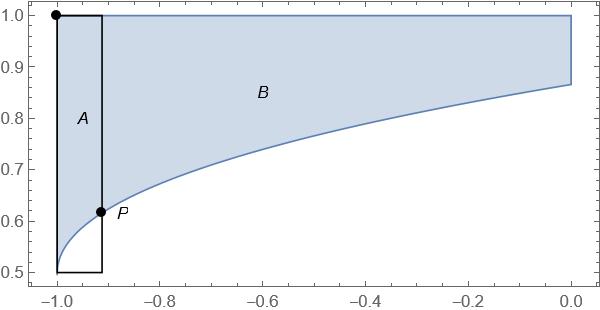
Figure 11: The figure depicts our strategy for showing $\tilde{F}\geq\tilde{g}$ in the large $a$ case. We show $\tilde{F}\leq\tilde{g}$ on the rectangular region A (which includes points outside of $\tilde{\Delta}_{A_{2}}$) in Lemma 21. The remaining points of $\tilde{\Delta}_{A_{2}}$, in region B, are handled by Lemma 22.

We begin by showing that $\tilde{F}\geq\tilde{g}$ on two segments of the boundary or $\tilde{\Delta}_{A_{2}}$.

Lemma 19.

We have $\tilde{F}\geq\tilde{g}$ on the set $\{(-1,t_{2}):t_{2}\in[1/2,1]\}\cup\{(t_{1},1):t_{1}\in[-1,1]\}$ with equality only at $(-1,1)$.

Proof.

For the segment $\{(-1,t_{2}):t_{2}\in[1/2,1]\}$, we prove in the appendix that for $a>21$,

$$\frac{\partial\tilde{F}}{\partial t_{1}}(-1,1)>\frac{\partial\tilde{F}}{\partial t_{2}}(-1,1)$$ (56)

It also holds for $0<a<21$ as an immediate consequence of Lemma 18. We next show for $a>21$ that $(\tilde{F}-\tilde{g})(-1,1/2)>0$, and so using the definition

$$b_{1}=\frac{\partial\tilde{F}}{\partial t_{2}}(-1,1),$$

for this range of $a$, we may apply Lemma 17 to obtain $\tilde{F}\geq\tilde{g}$ on $\{(-1,t_{2}):t_{2}\in[1/2,1]\}$ with equality only at $(-1,1)$. Now for the other segment, we simply apply (56), our definition of $b_{1}$, and the convexity of $\tilde{F}-\tilde{g}$ in $t_{1}$. ∎

Next, we show that $\tilde{F}(t_{1},t_{2})\geq\tilde{g}(t_{1},t_{2})$ in $\tilde{\Delta}_{A_{2}}$ if $t_{1}\leq\cos(2\pi\frac{\sqrt{3}}{4})$ with equality only at $(-1,1)$, and in fact we’ll show the stronger claim that $\tilde{F}\geq\tilde{g}$ on all of $A:=[-1,\cos(2\pi\frac{\sqrt{3}}{4})]\times[1/2,1]$ (see Figure 11) with equality only at $(-1,1)$.
Let $H_{\tilde{F}}$ denote the Hessian matrix of $\tilde{F}$. It follows from the strict complete monotonicity of the log derivative of $\tilde{\theta}$ that $\tilde{f}_{i}^{\prime\prime}\tilde{f}_{i}<(\tilde{f}_{i}^{\prime})^{2}$ for $i\in\{1,2\}$ (see Proposition 10), and hence we have

$$\det(H_{\tilde{F}} (t_{1},t_{2}))=(\tilde{f_{1}}^{\prime\prime}(t_{1})\tilde{f_{1}}(t_{1}))(\tilde{f_{2}}^{\prime\prime}(t_{2})\tilde{f_{2}}(t_{2}))-\tilde{f_{1}}^{\prime}(t_{1})^{2}\tilde{f_{2}}^{\prime}(t_{2})^{2}+$$

$$(\tilde{f_{1}}^{\prime\prime}(-t_{1})\tilde{f_{1}}(-t_{1}))(\tilde{f_{2}}^{\prime\prime}(-t_{2})\tilde{f_{2}}(-t_{2}))-\tilde{f_{1}}^{\prime}(-t_{1})^{2}\tilde{f_{2}}^{\prime}(-t_{2})^{2}<0$$

for $t_{1},t_{2}\in[-1,1].$

To establish that $\tilde{F}\geq\tilde{g}$ on a rectangle $R\subset[-1,1]^{2}$ with upper left corner point $(c,d)$ (we subdivide the rectangle $A$ into three such rectangles in the proof of Lemma 21), we introduce the following auxiliary function

$$\tilde{g}_{c,d}(t_{1},t_{2}):=\tilde{g}(t_{1},t_{2})-b_{1}t_{1}t_{2}+b_{1}(ct_{2}+dt_{1}-cd),$$ (57)

and observe that $t_{1}t_{2}\leq ct_{2}+dt_{1}-cd$ for $t_{1}\geq c$, $t_{2}\leq d$, and so

$$\tilde{g}(t_{1},t_{2})\leq\tilde{g}_{c,d}(t_{1},t_{2})\quad t_{1}\geq c,\,t_{2}\leq d$$ (58)

with equality if and only if $t_{1}=c$ or $t_{2}=d$. We further observe that

$$\det(H_{\tilde{F}-\tilde{g}_{c,d}})=\det(H_{\tilde{F}})-2b_{1}\tilde{f_{1}}^{\prime\prime}(t_{1})\tilde{f_{2}}(t_{2})<\det(H_{\tilde{F}})<0.$$

Hence, to verify $\tilde{F}\geq\tilde{g}$ on the rectangle $R$, it suffices to show $\tilde{F}\geq\tilde{g}_{c,d}$ on the boundary of the region by the second derivative test. For the two sides of the rectangle where $t_{1}=c$ and $t_{2}=d$, we will have already established $\tilde{F}\geq\tilde{g}$, and since $\tilde{g}=\tilde{g}_{c,d}$ on those sides, we immediately obtain $\tilde{F}\geq\tilde{g}_{c,d}$ there.

On the other two sides, we reduce the $a\geq 21$ case to just $a=21$ in the following way. In each case, using truncated series approximations of $\theta$ and $b_{1}$ developed in the appendix, we find an upper bound on $\tilde{g}_{c,d}^{*}\geq\tilde{g}_{c,d}$ with the key feature that $e^{a/4}\tilde{g}_{c,d}^{*}$ is linear in $a$. Meanwhile, as a lower bound for $\tilde{F}$, we truncate the expansions for $f_{1}$ and $f_{2}$ from (21) to obtain

$$\tilde{F}_{T}(t_{1},t_{2}):=(e^{-ax^{2}}+e^{-a(x-1)^{2}})e^{-3au^{2}}+e^{-a((\frac{1}{2}-x)^{2}+3(\frac{1}{2}-u)^{2})}<\tilde{F}(t_{1},t_{2}),\qquad t_{1},t_{2}\in[-1,1],$$ (59)

where

$$x=\frac{\arccos(t_{1})}{2\pi},\hskip 14.22636ptu=\frac{\arccos(t_{2})}{2\pi}.$$ (60)

It is straightforward to verify that $e^{a/4}\tilde{F}_{T}(t_{1},t_{2})$ is convex in $a$ for any fixed $(t_{1},t_{2})$ and so the difference $e^{a/4}(\tilde{F}_{T}-\tilde{g}_{c,d}^{*})$ is also (pointwise) convex in $a$. Thus, to establish $\tilde{F}_{T}\geq\tilde{g}_{c,d}^{*}$ at some point $(t_{1},t_{2})$ for all $a\geq 21$ it suffices to show

$$\begin{split}(\tilde{F}_{T}-\tilde{g}_{c,d}^{*})(t_{1},t_{2})\bigg{|}_{a=21}&\geq 0\\ \frac{\partial\left[e^{a/4}(\tilde{F}_{T}-\tilde{g}_{c,d}^{*})(t_{1},t_{2})\right]}{\partial a}\bigg{|}_{a=21}&\geq 0.\end{split}$$ (61)

In short, to establish $\tilde{F}\geq\tilde{g}$ on a rectangle $R$ with upper left vertex $(c,d)$ for which we have already established this inequality on the left and upper edges, it suffices to establish the inequalities (61) for $(t_{1},t_{2})$ on the two bottom and right line segments bounding $R$. Moreover, since the above method actually establishes $\tilde{F}\geq\tilde{g}^{*}_{c,d}$, we have the strict inequality $\tilde{F}>\tilde{g}$ on the whole rectangle except for possibly points where $t_{1}=c$ or $t_{2}=d$. We summarize our discussion in the following lemma which will be helpful in the 6-point case.

Lemma 20.

Let $R:[c,c^{\prime}]\times[d^{\prime},d]\subseteq[-1,1]^{2}$ be a rectangle with upper left corner point $(c,d)$, and further suppose that there exist functions $\tilde{g},\tilde{g}_{c,d},\tilde{g}_{c,d}^{*},\tilde{F}_{T},$ and $\tilde{F}$ of the variables $(a,t_{1},t_{2})\in(0,\infty)\times[0,1]^{2}$ with continuous 2nd order partial derivatives which satisfy for all $a\geq a^{\prime}$:

1. $\tilde{g}\leq\tilde{g}_{c,d}\leq\tilde{g}_{c,d}^{*}$ on $R$ with $\tilde{g}=\tilde{g}_{c,d}$ if and only if $t_{1}=c$ or $t_{2}=d$

2. $\tilde{F}_{T}\leq\tilde{F}$ on $R$

3. $\det{H_{\tilde{F}-\tilde{g}_{c,d}^{*}}}<0$ on $R$

4. For some $m_{1}$, $e^{a/m_{1}}(\tilde{F}-\tilde{g}_{c,d})$ is pointwise convex in the parameter $a$

If there is some $a^{\prime}>0$ such that the inequalities

$$\begin{split}(\tilde{F}_{T}-\tilde{g}_{c,d}^{*})(t_{1},t_{2})\bigg{|}_{a=a^{\prime}}&\geq 0\\ \frac{\partial\left[e^{a/m_{1}}(\tilde{F}_{T}-\tilde{g}_{c,d}^{*})(t_{1},t_{2})\right]}{\partial a}\bigg{|}_{a=a^{\prime}}&\geq 0\end{split}$$ (62)

hold on $\partial R$, then $\tilde{F}>\tilde{g}$ on $R$ for all $a\geq a^{\prime}$. Further, if for all $a\geq a^{\prime}$, $\tilde{F}\geq\tilde{g}$ on some $R^{\prime}\subseteq\{(t_{1},t_{2})\in\partial R:t_{1}=c\text{ or }t_{2}=d\}$ and the inequalities (62) hold on $\partial R\backslash R^{\prime}$, then $\tilde{F}\geq\tilde{g}$ on $R$ for all $a\geq a^{\prime}$, again with equality only possible if $t_{1}=c$ or $t_{2}=d$ and $(t_{1},t_{2})\in R^{\prime}$.

Lemma 21.

The inequality $\tilde{F}\geq\tilde{g}$ holds on $A=[-1,\cos(2\pi\frac{\sqrt{3}}{4})]\times[\frac{1}{2},1]$ with equality only at $(-1,1)$.

Proof.

We partition $[-1,\cos(2\pi\frac{\sqrt{3}}{4})]\times[\frac{1}{2},1]$ into three subrectangles $R_{k}:=[-1,\cos(2\pi\frac{\sqrt{3}}{4})]\times[d_{k-1},d_{k}]$, $k=1,2,3$ where $d_{0}=1/2$, $d_{1}=3/5$, $d_{2}=7/10$, and $d_{3}=1$ and aim to verify the inequality $\tilde{F}\geq\tilde{g}_{-1,d_{k}}$ on each $R_{k}$ using Lemma 20, with $\tilde{g}_{-1,d_{k}}$ as in (57), $\tilde{F}_{T}$ as in (59), $m_{1}=4$, and $a^{\prime}=21$. The specific formulas for each $g_{-1,d_{k}}^{*}$ are given in the appendix section D.3. We begin by verifying inequalities (62) for $g_{-1,-1}^{*}$ on the line segments of $R_{1}$ with $t_{1}=\cos(2\pi\sqrt{3}/4)$ or $t_{2}=7/10$, which combined with Lemma 20 implies $\tilde{F}\geq\tilde{g}$ on $R_{1}$. Now having established $\tilde{F}\geq\tilde{g}$ on the top side of $R_{2}$, we only need establish inequalities (62) for $g_{-1,-1}^{*}$ on the line segments of $R_{2}$ where $t_{1}=\cos(2\pi\sqrt{3}/4)$ or $t_{2}=3/5$ to get $\tilde{F}\geq\tilde{g}$ on all $R_{2}$. In the same fashion, showing inequalities (62) on the sides of $R_{3}$ where $t_{1}=\cos(2\pi\sqrt{3}/4)$ or $t_{2}=3/5$ completes the proof by yielding $\tilde{F}\geq\tilde{g}$ on $R_{3}$. The verification of these inequalities is carried out in the appendix by reducing them to inequalities of the form $h_{2}(t)-h_{1}(t)>0$ on an interval $(\alpha,\beta)$ where $h_{1}$ and $h_{2}$ are increasing functions and choose $\delta:=(\beta-\alpha)/n$ with sufficiently large that we may rigorously verify the inequalities

$$h_{1}(\alpha+k\delta)<h_{2}(\alpha+(k-1)\delta),\qquad k=1,2,\ldots,n,$$ (63)

thereby reducing our check to a finite number of point evaluations. ∎

Finally, we show that $\tilde{F}-\tilde{g}$ increases in $t_{1}$ for every point in $\tilde{\Delta}_{A_{2}}$ with $t_{1}\geq\cos(2\pi\frac{\sqrt{3}}{4})$, thus completing the proof for the $a>21$ case and yielding $\tilde{F}\geq\tilde{g}$ on all $\tilde{\Delta}_{A_{2}}$ with equality only at $(-1,1)$.

Lemma 22.

For all $a\geq 21$ and every $p=(t_{1},t_{2})\in\tilde{\Delta}_{A_{2}}$ with $t_{1}\geq\cos(2\pi\frac{\sqrt{3}}{4})$, $\frac{\partial(\tilde{F}-\tilde{g})}{\partial t_{1}}\bigg{|}_{p}\geq 0$.

Proof.

Because of the convexity of the difference in $t_{1}$ and Lemma 16, it suffices to show that at $P=(\cos(2\pi\frac{\sqrt{3}}{4}),\cos(2\pi\frac{\sqrt{3}}{12}))$,

$$\frac{\partial(\tilde{F}-\tilde{g})}{\partial t_{1}}\bigg{|}_{P}\geq 0,\hskip 28.45274pt\frac{\partial^{2}(\tilde{F}-\tilde{g})}{\partial t_{1}\partial t_{2}}\bigg{|}_{P}\geq 0$$ (64)

which is handled in the appendix. ∎

5 $L$-universal optimality of $\omega^{*}_{6}$

We consider the $m=1$ case of the interpolation problem from Section 3.6. In this case we have interpolation conditions at the nodes $\tilde{\tau}_{6}=\{(-1,-1),(1,-\frac{1}{2}),(-1,\frac{1}{2})\}$. Using the same rescaling convention as in the previous section, we have

$$\tilde{F}(t_{1},t_{2})=\tilde{f_{1}}(t_{1})\tilde{f_{2}}(t_{2}),$$

where $\tilde{f_{1}},\tilde{f_{2}}$ are as in (52). For $m=1$, we may choose an interpolant $\tilde{g}=\tilde{g}_{a}\in\mathcal{P}_{1}(t_{1})\times\mathcal{P}_{2}(t_{2})$; i.e $\tilde{g}$ of the form

$$\tilde{g}(t_{1},t_{2})=\sum_{i=0}^{1}\sum_{j=0}^{2}b_{i,j}t_{1}^{i}t_{2}^{j}.$$

We require that $\tilde{g}$ and $\tilde{F}$ agree at the three points in $\tilde{\tau}_{6}$ and remark that the condition $\tilde{g}\leq\tilde{F}$ further requires $\partial\tilde{g}/\partial t_{2}=\partial\tilde{F}/\partial t_{2}$ at the points $(-1,1/2)$ and $(1,-1/2)$ giving a total of 5 linearly independent conditions on $\mathcal{P}_{1}(t_{1})\times\mathcal{P}_{2}(t_{2})$.

Figure 12: $\tilde{g}$ has 5 necessary equality interpolation conditions in order to provide a sharp bound, the 3 value conditions from $\tilde{\tau}_{6}$, plus two derivative conditions.

Noting that $q(t_{1},t_{2})=(1+t_{1})(t_{2}+1/2)^{2}$ vanishes on $\tilde{\tau}_{6}$ and that $\frac{\partial q}{\partial t_{2}}$ vanishes on $\{(-1,1/2),(1,-1/2)\}$ shows that $\tilde{g}$ can be written as

$$\begin{split}\tilde{g}(t_{1},t_{2})&=\frac{(1-t_{1})}{2}\tilde{f_{1}}(-1)H_{\{-1,\frac{1}{2},\frac{1}{2}\}}(\tilde{f_{2}})(t_{2})+\frac{(1+t_{1})}{2}\tilde{f_{1}}(1)H_{\{-\frac{1}{2},-\frac{1}{2}\}}(\tilde{f_{2}})(t_{2})+cq(t_{1},t_{2}),\end{split}$$ (65)

where $H_{T}(f)$ is the Hermite interpolant to $f$ on the node set $T$ which can be expressed in terms of divided differences (see Appendix A). In particular,

$$H_{\{-1,\frac{1}{2},\frac{1}{2}\}}(\tilde{f_{2}})(t_{2})=\tilde{f_{2}}(-1)+\tilde{f_{2}}[-1,\frac{1}{2}](t_{2}+1)+\tilde{f_{2}}[-1,\frac{1}{2},\frac{1}{2}](t_{2}+1)(t_{2}-\frac{1}{2}),$$

and $H_{\{-\frac{1}{2},-\frac{1}{2}\}}(\tilde{f_{2}})(t_{2})=\tilde{f_{2}}(-\frac{1}{2})+\tilde{f_{2}}^{\prime}(-\frac{1}{2})(t_{2}+\frac{1}{2})^{2}$. Since $T_{1}(t)=t$ and $T_{2}(t)=2t^{2}-1$, it easily follows that $\tilde{g}$ is CPSD if and only if $b_{i,j}\geq 0$ for $(i,j)\neq 0$. From (65), it follows that $b_{1,2}=-\frac{1}{2}\tilde{f_{1}}(-1)\tilde{f_{2}}[-1,\frac{1}{2},\frac{1}{2}]+c$. Observing that $q\geq 0$ on $[-1,1]^{2}$, we choose $c=\frac{1}{2}\tilde{f_{1}}(-1)\tilde{f_{2}}[-1,\frac{1}{2},\frac{1}{2}]$ as small as possible in which case $b_{1,2}=0$.

In addition, the following derivative equality,

$$\tilde{f_{1}}(-1)\tilde{f_{2}}^{\prime}(1/2)=\tilde{f_{1}}(1)\tilde{f_{2}}^{\prime}(-1/2).$$ (66)

proved in [1] (also see [33]) implies that $b_{1,1}=b_{0,2}$. Hence we may express $\tilde{g}$ in the form

$$\tilde{g}(t_{1},t_{2})=a_{0,0}+a_{1,0}t_{1}+a_{0,1}t_{2}+a_{0,2}(t_{1}t_{2}+t^{2}_{2}+1/4),$$ (67)

where $a_{0,0}=b_{0,0}-b_{0,2}/4$ and $a_{i,j}=b_{i,j}$ otherwise.

From (65), we then compute

$$\begin{split}a_{0,0}&=\frac{\tilde{f_{1}}(1)\tilde{f_{2}}(-1/2)+\tilde{f_{1}}(-1)\tilde{f_{2}}(1/2)}{2}\\ a_{0,1}&=\tilde{f_{1}}(-1)\tilde{f_{2}}^{\prime}(-1/2)\\ a_{1,0}&=\frac{\tilde{f_{1}}(1)\tilde{f_{2}}(-1/2)-\tilde{f_{1}}(-1)\tilde{f_{2}}(1/2)}{2}+\frac{a_{0,1}}{2}\\ a_{0,2}&=\tilde{f_{1}}(-1)\tilde{f_{2}}[-1,\frac{1}{2},\frac{1}{2}]=\frac{4}{9}(\tilde{f_{1}}(-1)\tilde{f_{2}}(-1)+a_{0,1}+a_{1,0}-a_{0,0}).\end{split}$$ (68)

The strict absolute monotonicity and positivity of $\tilde{f_{2}}$ and $\tilde{f_{1}}$ show that the coefficients $a_{0,0},a_{0,1}$, and $a_{0,2}$ in (68) are positive.

The next lemma which will be used to prove $a_{1,0}>0$ as well as being a first step in establishing that $\tilde{g}\leq\tilde{F}$ on $[-1,1]^{2}$.

Lemma 23.

$\tilde{F}(-1,t_{2})\geq\tilde{g}(-1,t_{2})$ for all $t_{2}\in[-1,1]$ with equality only if $t_{2}\in\{-1,1/2\}$.

Proof.

The result follows from the error formula (81) applied to the strictly absolute monotone function $\tilde{F}(-1,t_{2})=\tilde{f_{1}}(-1)\tilde{f_{2}}(t_{2})$ for $t_{2}$ on [-1,1]. ∎

It remains to show that $a_{1,0}>0$.

Proposition 24.

The coefficients $a_{0,0},a_{0,1},a_{1,0}$, and $a_{0,2}$ are positive. Hence, $\tilde{g}$ is CPSD.

Proof.

By Lemma 23, $\tilde{g}(-1,-1/2)<\tilde{F}(-1,-1/2)$. Moreover, by definition, $\tilde{g}(1,-1/2)=\tilde{F}(1,-1/2)$. Since $(\tilde{F}-\tilde{g})(t_{1},-1/2)$ is convex in $t_{1}$, we must have

$$a_{1,0}-\frac{1}{2}a_{0,2}=\frac{\partial\tilde{g}}{\partial t_{1}}(-1,-1/2)\geq\frac{\partial\tilde{F}}{\partial t_{1}}(-1,-1/2)>0.$$ (69)

So $a_{1,0}-\frac{1}{2}a_{0,2}>0$ which implies $a_{1,0}>0$ since $a_{0,2}>0$. ∎

As in the proof of universal optimality of $\omega_{4}^{*}$ the most technical part of our proof is to verify $\tilde{g}\leq\tilde{F}$. In the remainder of Section 5, we reduce the proof of this inequality to a number of technical computations and estimates that are carried out in the Appendices C and D.

5.1 $\tilde{F}\geq\tilde{g}$ on $[-1,1]\times([-1,-1/2]\cup[1/2,1])$

The following lemma, proved in the appendix, establishes several necessary inequality conditions for $\tilde{g}\leq\tilde{F}$. We next show the inequality holds on $[-1,1]\times([-1,-1/2]\cup[1/2,1])$.

Lemma 25.

The following derivative conditions hold

$$\frac{\partial(\tilde{F}-\tilde{g})}{\partial t_{1}}(-1,-1)>0,$$ (70)

$$\frac{\partial(\tilde{F}-\tilde{g})}{\partial t_{1}}(-1,1/2)>0,$$ (71)

$$\frac{\partial(\tilde{F}-\tilde{g})}{\partial t_{1}}(1,-1/2)<0.$$ (72)

For fixed $t_{2}$, $\tilde{F}(t_{1},t_{2})-\tilde{g}(t_{1},t_{2})$ is strictly convex on $[-1,1]$ as a function of $t_{1}$ since $\tilde{g}(t_{1},t_{2})$ is linear in $t_{1}$ and $\tilde{f_{1}}$ is strictly absolutely monotone. The next proposition is an immediate consequence of this observation.

Lemma 26.

Let $t_{2}\in[-1,1]$. If either condition

1. $\frac{\partial(\tilde{F}-\tilde{g})}{\partial t_{1}}(-1,t_{2})\geq 0$ and $\tilde{F}(-1,t_{2})\geq\tilde{g}(-1,t_{2})$ or

2. $\frac{\partial(\tilde{F}-\tilde{g})}{\partial t_{1}}(1,t_{2})\leq 0$ and $\tilde{F}(1,t_{2})\geq\tilde{g}(1,t_{2})$

holds, then

$$\tilde{F}(t_{1},t_{2})\geq\tilde{g}(t_{1},t_{2}),\qquad t_{1}\in[-1,1].$$ (73)

If condition (a) holds, then we have strict inequality in (73) for $t_{1}\neq-1$. If condition (b) holds, then we have strict inequality in (73) for $t_{1}\neq 1$.

We use the above lemmas to obtain:

Lemma 27.

We have $\tilde{F}\geq\tilde{g}$ on $[-1,1]\times[1/2,1]$ with equality only at $(-1,1/2)$.

Proof.

We first note that $\frac{\partial(\tilde{F}-\tilde{g})}{\partial t_{1}}(t_{1},t_{2})=\tilde{f_{1}}^{\prime}(t_{1})\tilde{f_{2}}(t_{2})-a_{1,0}-a_{0,2}t_{2}$ is (a) strictly increasing in $t_{1}$ for fixed $t_{2}$ and (b) strictly convex in $t_{2}$ for fixed $t_{1}$. Let $h(t_{2}):=\frac{\partial(\tilde{F}-\tilde{g})}{\partial t_{1}}(-1,t_{2})$. The inequality (72) together with (a) implies $h(-1/2)<0$. Hence, the strict convexity of $h$ together with $h(1/2)>0$ (from (71)) implies $h(t_{2})=\frac{\partial(\tilde{F}-\tilde{g})}{\partial t_{1}}(-1,t_{2})>0$ for $t_{2}\in[1/2,1].$ Combining this fact with Lemma 23, we may invoke Lemma 26 part (a) to complete the proof. ∎

Next, we establish that $\tilde{F}\geq\tilde{g}$ on the right-hand boundary $t_{1}=1$.

Lemma 28.

We have $\tilde{F}(1,t_{2})\geq\tilde{g}(1,t_{2})$ for all $t_{2}\in[-1,1]$ with equality only at $t_{2}=-1/2$.

Proof.

Suppose by way of contradiction that there exists $t_{2}^{\prime}\in[-1,1]$ such that $t_{2}^{\prime}\neq-\frac{1}{2}$ and $\tilde{F}(1,t_{2}^{\prime})\leq\tilde{g}(1,t_{2}^{\prime})$. Then there must be some point $-1/2\neq p\in[-1,1]$ such that $\tilde{f_{1}}(1)\tilde{f_{2}}(p)=\tilde{g}(1,p)$. Indeed, either $t_{2}^{\prime}$ is such a point, or $\tilde{F}(1,t_{2}^{\prime})<\tilde{g}(1,t_{2}^{\prime})$. We have from Lemmas 25, 26, and 27 that $\tilde{F}(1,\pm 1)>\tilde{g}(1,\pm 1)$, which yield two cases for $t_{2}^{\prime}$. If $t_{2}^{\prime}<-1/2$, then there exists $p\in(-1,t_{2}^{\prime})$ such that $\tilde{F}(1,p)=\tilde{g}(1,p)$ by the intermediate value theorem. If $t_{2}^{\prime}>-1/2$, instead apply the intermediate value theorem on the interval $[t_{2}^{\prime},1]$ to see that $p\in[1/2,1]$.

Then $\tilde{g}(1,t_{2})$ is the unique quadratic polynomial that interpolates the function $\tilde{F}(1,t_{2})$ at $T=\{p,-1/2,-1/2\}$. Then the error formula (81) gives

$$\tilde{F}(1,t_{2})-\tilde{g}(1,t_{2})=\tilde{f_{1}}(1)\tilde{f_{2}}^{(3)}(\xi)(t_{2}-p)(t_{2}+1/2)^{2}$$

for some $\xi\in[-1,1]$. The positivity of $\tilde{f_{2}}^{(3)}$ then implies the contradiction $\tilde{F}(1,-1)=\tilde{f_{1}}(1)\tilde{f_{2}}(-1)<\tilde{g}(1,-1)$ completing the proof. ∎

Lemma 29.

We have $\tilde{F}\geq\tilde{g}$ on $[-1,1]\times[-1,-1/2]$ with equality only at $(-1,-1)$ and $(1,-1/2)$.

Proof.

From Lemma 23, we have $\tilde{F}\geq\tilde{g}$ for $t_{1}=-1$. By Lemmas 25 and 26, we have the same inequality when $t_{2}=-1/2$ or $-1$. Finally, by Lemma 28, we have the inequality for $t_{1}=1$. All of these inequalities are strict except for at $(-1,-1)$ and $(1,-1/2)$.

Let $p=(p_{1},p_{2})$ be an arbitrary point on the boundary of $[-1,1]\times[-1,-1/2]$ such that $p_{1}<1$ and $p_{2}<-1/2$, let $q=(1,-1/2)$, and let $l(s):=p+s(q-p)$, $0\leq s\leq 1$, parametrize the line segment from $p$ to $q$. Since $u_{l}:=q-p$ has positive components, it follows that $\tilde{F}^{l}:=\tilde{F}\circ l$ is strictly absolutely monotone on $[0,1]$. Also, let $\tilde{g}^{l}:=\tilde{g}\circ l$ and note that $\tilde{g}^{l}$ is a polynomial of degree at most 2.

We claim that $(\tilde{F}^{l}-\tilde{g}^{l})(\epsilon)>0$ for all sufficiently small $\epsilon>0$. Indeed, if $p\neq(-1,-1)$, then $(\tilde{F}^{l}-\tilde{g}^{l})(0)>0$ and the result follows by continuity. If $p=(-1,-1)$, then $\nabla(\tilde{F}-\tilde{g})(-1,-1)\cdot u_{l}>0$ at (-1,-1) by Lemmas 25 and 23 which shows the result in this case. Similarly, the necessary derivative inequality and equality conditions at $(1,-1/2)$ imply $\nabla(\tilde{F}-\tilde{g})(-1,1/2)\cdot u_{l}<0$. Together with the fact that $(\tilde{F}^{l}-\tilde{g}^{l})(1)=0$, we get $(\tilde{F}^{l}-\tilde{g}^{l})(1-\epsilon)>0$ for all $\epsilon$ sufficiently small.

Now supposing for a contradiction that $(\tilde{F}^{l}-\tilde{g}^{l})(r^{\prime})<0$ for some $r^{\prime}\in(0,1)$. By the intermediate value theorem there are points $0<r_{1}<r^{\prime}<r_{2}<1$ such that $(\tilde{F}^{l}-\tilde{g}^{l})(r_{1})=(\tilde{F}^{l}-\tilde{g}^{l})(r_{2})=0$. Then $\tilde{g}^{l}$ is a polynomial of degree at most 2 which interpolates $\tilde{F}^{l}$ for $T=\{r_{1},r_{2},1\}$ and leads to a contradiction using the error formula (81). Since any point in $(-1,1)\times(-1,-1/2)$ must lie on such a line segment, we conclude that $\tilde{F}\geq\tilde{g}$ on $(-1,1)\times(-1,-1/2)$. Now to see the inequality must be strict, if $(\tilde{F}^{l}-\tilde{g}^{l})(r^{\prime})=0$ for some $r^{\prime}\in(0,1)$ $\tilde{g}^{l}$ is a polynomial of degree at most 2 which interpolates $\tilde{F}^{l}$ for $T=\{r^{\prime},r^{\prime},1\}$, and again we obtain a contradiction with the error formula. ∎

Thus, we have proved $\tilde{F}\geq\tilde{g}$ on $[-1,1]^{2}$ whenever $t_{2}\geq 1/2$ or $t_{2}\leq-1/2$. Our proof of the inequality for the critical region $-1/2\leq t_{2}\leq 1/2$ is more delicate and requires different approaches for $a$ small and $a$ large.

5.2 The critical region for small $a$ ($a<\pi^{2}$)

For $a<\pi^{2}$, we take a linear approximation approach. Let

$$L_{\pm 1}(t_{1},t_{2}):=(\tilde{F}-\tilde{g})(\pm 1,t_{2})+(t_{1}\mp 1)\frac{\partial(\tilde{F}-\tilde{g})}{\partial t_{1}}(\pm 1,t_{2})$$

denote the tangent approximation of $\tilde{F}-\tilde{g}$ for fixed $t_{2}$ about $t_{1}=\pm 1$. Since $(\tilde{F}-\tilde{g})(t_{1},t_{2})$ is strictly convex in $t_{1}$ for fixed $t_{2}$, we have

$$\small(\tilde{F}-\tilde{g})(t_{1},t_{2})\geq\max\{L_{-1}(t_{1},t_{2}),L_{-1}(t_{1},t_{2})\}\geq\min\{L_{-1}(-1,t_{2}),L_{-1}(0,t_{2}),L_{1}(0,t_{2}),L_{1}(1,t_{2})\},$$ (74)

where the second inequality uses that $L_{\pm 1}(t_{1},t_{2})$ is a linear polynomial in $t_{1}$ for fixed $t_{2}$. Note the first inequality in (74) is strict if $-1<t_{1}<1$.

Now $L_{-1}(-1,t_{2})=(\tilde{F}-\tilde{g})(-1,t_{2})\geq 0$ by Lemma 23 and $L_{1}(1,t_{2})=(\tilde{F}-\tilde{g})(1,t_{2})\geq 0$ by Lemma 28. In fact, we shall next prove that $L_{-1}(0,t_{2})\geq L_{1}(0,t_{2})$ so that the minimum on the right-hand side of (74) is non-negative if $L_{1}(0,t_{2})$ is non-negative.

Lemma 30.

If $t_{2}\in(-1,1)$, then $L_{-1}(0,t_{2})>L_{1}(0,t_{2})$.

Proof.

Since $\tilde{g}$ is affine in $t_{1}$, we have

$$L_{\pm 1}(0,t_{2}):=\tilde{F}(\pm 1,t_{2})\mp\frac{\partial\tilde{F}}{\partial t_{1}}(\pm 1,t_{2})-\tilde{g}(0,t_{2}).$$ (75)

Then, the error formula (81) applied to $\tilde{F}(\cdot,t_{2})$ (or the Lagrange remainder formula) gives

$$\tilde{F}(0,t_{2})=\tilde{F}(\pm 1,t_{2})\mp\frac{\partial\tilde{F}}{\partial t_{1}}(\pm 1,t_{2})+\frac{1}{2}\tilde{f_{1}}^{\prime\prime}(\chi_{\pm})\tilde{f_{2}}(t_{2}),$$

where $-1<\chi_{-}<0<\chi_{+}<1$ which with (75) and the absolute monotonicity of $\tilde{f_{1}}$ implies

$$L_{-1}(0,t_{2})=\tilde{F}(0,t_{2})-\frac{1}{2}\tilde{f_{1}}^{\prime\prime}(\chi_{-})\tilde{f_{2}}(t_{2})>\tilde{F}(0,t_{2})-\frac{1}{2}\tilde{f_{1}}^{\prime\prime}(\chi_{+})\tilde{f_{2}}(t_{2})=L_{1}(0,t_{2}).$$

∎

Hence, if

$$\phi(t_{2}):=L_{1}(0,t_{2})\geq 0,$$

then (75) and Lemma 74 show $(\tilde{F}-\tilde{g})(t_{1},t_{2})>0$ for all $-1<t_{1}<1.$ So it suffices to show $\phi\geq 0$ on $[-1/2,1/2]$ to prove that $\tilde{g}\leq\tilde{F}$ on the critical region. We can express $\phi(t_{2})$ as

$$\phi(t_{2})=(\tilde{f_{1}}(1)-\tilde{f_{1}}^{\prime}(1))\tilde{f_{2}}(t_{2})-a_{0,0}-a_{0,1}t_{2}-a_{0,2}(t_{2}^{2}+1/4).$$

Using our technical bounds on $\tilde{\theta}$, we show the following lemma in the appendix:

Lemma 31.

For $a<\pi^{2}$, $\tilde{f_{1}}(1)-\tilde{f_{1}}^{\prime}(1)\geq 0$.

Thus, $\phi^{(3)}(t_{2})\geq 0$, and so its 2nd degree Taylor polynomial at $t_{2}=-1/2$ yields the following lower bound for $t_{2}\geq-1/2$:

$$\phi(t_{2})\geq A+B(t_{2}+1/2)+\frac{C}{2}(t_{2}+1/2)^{2}$$

where $A=\phi(-1/2)$, $B=\phi^{\prime}(-1/2)$, and $C=\phi^{\prime\prime}(-1/2)$. In the appendix (see Section C.3.2), we prove

Lemma 32.

For $a<\pi^{2}$, $A,C>0$. If $B<0$, then $B^{2}-2AC<0$.

It follows from Lemma 32 that $A+B(t_{2}+1/2)+\frac{C}{2}(t_{2}+1/2)^{2}>0$ for $t_{2}\geq-1/2$ completing the proof that $\tilde{g}\leq\tilde{F}$ in the case $a<\pi^{2}$, and moreover, showing that $\tilde{F}=\tilde{g}$ only at our interpolation points $(-1,1),(-1,1/2),(1,-1/2)$.

5.3 The critical region for $a\geq 9.6$

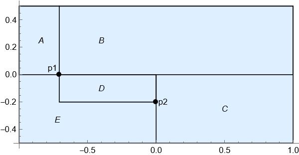
Figure 13: The figure depicts our proof strategy for showing $\tilde{F}\geq\tilde{g}$ on the critical region when $a$ is large. The points $p_{1}$ and $p_{2}$ are located at $(-\sqrt{2}/2,0),(0,-1/5)$, respectively.

To complete the proof of universal optimality of $\omega^{*}_{6}$, it remains to show that $\tilde{F}\geq\tilde{g}$ on the critical region when $a>\pi^{2}$. In fact, we will show the inequality is strict on the interior of the critical region. We split the region into several subregions as in Figure 13. The inequality $\tilde{F}\geq\tilde{g}$ for Subregions A,B,C,D, and E from Figure 13 is handled in Lemmas 33, 34, 35, 36, and 37, respectively.

To prove $\tilde{F}\geq\tilde{g}$ on the regions $A$ and $D$, we apply Lemma 20. Here we use

$$\tilde{g}_{c,d}(t_{1},t_{2}):=\tilde{g}(t_{1},t_{2})+a_{0,2}(-t_{1}t_{2}+ct_{2}+dt_{1}-cd)$$

for $c,d\in[-1,1]$. Approximating the coefficients $a_{i,j}$ for $a\geq a^{\prime}:=9.6$, we obtain $\tilde{g}_{c,d}^{*}$ such that $\tilde{g}_{c,d}^{*}\geq\tilde{g}_{c,d}$ on the relevant subrectangle and $e^{a/3}\tilde{g}_{c,d}^{*}$ is linear in $a$. See Section D.4.3 for the construction of $\tilde{g}_{c,d}^{*}$ in the different subrectangles. As a lower bound for $\tilde{F}$, we use

$$\tilde{F}_{T}:=(e^{-ax^{2}}+e^{-a(x-1)^{2}})e^{-3au^{2}}$$ (76)

where $x$ and $u$ are given in (60). Analogously to the 4-point case, it is straightforward to verify that these choices of $\tilde{F}_{T}$, $\tilde{g}_{c,d}$, and $\tilde{g}_{c,d}^{*}$ satisfy conditions 1–4 of Lemma 20 with $m_{1}=3$ and $a^{\prime}=9.6$.

Lemma 33.

We have $\tilde{F}\geq\tilde{g}$ on $A=[-1,-\sqrt{2}/2]\times[0,1/2]$ with equality only at $(-1,1/2)$.

Proof.

First, we show the inequality for $[-1,-\sqrt{2}/2]\times[1/4,1/2]$. Since we already have $\tilde{F}\geq\tilde{g}$ when $t_{2}=1/2$ or $t_{1}=-1$, it suffices by Lemma 20 to show inequalities (62) on the 2 segments when $t_{2}=1/4$ or $t_{1}=-\sqrt{2}/2$, which we handle in the appendix Section D.4.3. Now having $\tilde{F}\geq\tilde{g}$ on the segment of $[-1,-\sqrt{2}/2]\times[0,1/4]$ when $t_{2}=1/4$, we again show inequalities (62) with $\tilde{g}_{-1,1/4}$ on the segments when $t_{2}=0$ or $t_{1}=-\sqrt{2}/2$ to complete the proof.

∎

Lemma 34.

We have $\tilde{F}>\tilde{g}$ on $B=[-\sqrt{2}/2,1]\times[0,1/2]$.

Proof.

By the convexity of $\tilde{F}-\tilde{g}$ in $t_{1}$, it suffices to show:

1. $\tilde{F}(-\sqrt{2}/2,t_{2})\geq\tilde{g}(-\sqrt{2}/2,t_{2})$ for all $t_{2}\in[0,1/2]$

2. $\frac{\partial(\tilde{F}-\tilde{g})}{\partial t_{1}}(-\sqrt{2}/2,t_{2})\geq 0$ for $t_{2}\in[0,1/2]$.

The first of these follows from Lemma 33. To prove the second, it actually suffices to just show that $\frac{\partial(\tilde{F}-\tilde{g})}{\partial t_{1}}(-\sqrt{2}/2,0)\geq 0$, which is handled in the appendix section D.4.4. This sufficiency follows from the same reasoning as Lemma 27 and holds because $\frac{\partial(\tilde{F}-\tilde{g})}{\partial t_{1}}\geq 0$ is convex in $t_{2}$ and satisfies $\frac{\partial(\tilde{F}-\tilde{g})}{\partial t_{1}}(-\sqrt{2}/2,-1/2)<0$ (due to the necessary condition $\frac{\partial(\tilde{F}-\tilde{g})}{\partial t_{1}}(1,-1/2)<0$). ∎

Lemma 35.

We have $\tilde{F}\geq\tilde{g}$ on $C=[0,1]\times[-1/2,0]$ with equality only at $(1,-1/2)$.

Proof.

We claim that for this portion of the critical region, it suffices to show at each point that

$$L_{1}(t_{1},t_{2}):=\frac{\tilde{f_{2}}^{\prime}(t_{2})\tilde{f_{1}}(t_{1})}{\tilde{f_{1}}^{\prime}(t_{1})\tilde{f_{2}}(t_{2})}-\frac{\frac{\partial\tilde{g}}{\partial t_{2}}(t_{1},t_{2})}{\frac{\partial\tilde{g}}{\partial t_{1}}(t_{1},t_{2})}>0,$$

since this would imply that $\tilde{g}$ increases along the level curves of $\tilde{F}$ as $t_{1}$ increases.

Thus, $\tilde{F}-\tilde{g}$ is minimized along the right and bottom boundaries of the region, where we have already showed $\tilde{F}-\tilde{g}\geq 0$ in the previous section with equality only at $(1,-1/2)$. The inequality $L_{1}(t_{1},t_{2})>0$ for $(t_{1},t_{2})\in[0,1]\times[-1/2,0]$ is proved in the appendix section D.4.5. ∎

Lemma 36.

We have $\tilde{F}>\tilde{g}$ on $D=[-\sqrt{2}/2,0]\times[\frac{1}{5},0]$.

Proof.

We first show inequalities (62) hold for $\tilde{g}_{-\sqrt{2}/2,0}$ on each line segment on the boundary of $[-\sqrt{2}/2,0\times[-.1,0]$ except the $t_{2}=0$ segment (where we already have $\tilde{F}>\tilde{g}$). Then we repeat the process with $\tilde{g}_{-\sqrt{2}/2,-.1}$ on each segment of $[-\sqrt{2}/2,0]\times[-.2,-.1]$ except the $t_{2}=-.1$ segment. The precise calculations are carried out in the appendix section D.4.3.

∎

Lemma 37.

We have $\tilde{F}>\tilde{g}$ on $E=[-1,0]\times[-.5,-.2]\cup[-1,-\sqrt{2}/2]\times[-.5,0]$.

Proof.

We extend the domain of the $\log$ function so that $\log(t)=\infty$ for $t\leq 0$. Note that this definition and the fact that $\tilde{F}>0$ on all of $[-1,1]^{2}$ imply $\log(\tilde{F}/\tilde{g})>0$ on $E$ is equivalent to $\tilde{F}>\tilde{g}$ on $E$. Since we have already established that this inequality holds on $\partial E$, it suffices to show $\log(\tilde{F}/\tilde{g})$ takes no finite local minima on $S$, which we’ll do by showing that

$$\frac{\partial}{\partial t_{1}}\log\left(\frac{\tilde{F}}{\tilde{g}}\right)<0$$ (77)

on all of $E$ where $\tilde{g}>0$, or equivalently, that if $\tilde{g}(t_{1},t_{2})>0$, then

$$\frac{\tilde{f_{1}}(t_{1})}{\tilde{f_{1}}^{\prime}(t_{1})}-\frac{\tilde{g}(t_{1},t_{2})}{\frac{\partial\tilde{g}(t_{1},t_{2})}{\partial t_{1}}}=\frac{\tilde{f_{1}}(t_{1})}{\tilde{f_{1}}^{\prime}(t_{1})}-t_{1}-\frac{\tilde{g}(0,t_{2})}{a_{1,0}+a_{0,2}t_{2}}>0$$

since each of $\tilde{f_{1}},\tilde{f_{1}}^{\prime},\frac{\partial\tilde{g}}{\partial t_{1}}>0$ on $E$ (see Equation 69). Notably, $\frac{\tilde{f_{1}}(t_{1})}{\tilde{f_{1}}^{\prime}(t_{1})}-t_{1}$ is a function only in $t_{1}$, while $\frac{\tilde{g}(0,t_{2})}{a_{1,0}+a_{0,2}t_{2}}$ depends only on $t_{2}$. Let

$$L_{2}(t_{1},t_{2}):=\frac{\tilde{f_{1}}(t_{1})}{\tilde{f_{1}}^{\prime}(t_{1})}-t_{1}-\frac{\tilde{g}(0,t_{2})}{a_{1,0}+a_{0,2}t_{2}}.$$

We will next establish that on all of $E$, $L_{2}$ is decreasing in $t_{1}$ and $t_{2}$. Thus to show $L_{2}>0$ on all of $E$, we need only check that $L_{2}(-\sqrt{2}/2,0),L_{2}(0,-.2)>0$, which is handled in the appendix section D.4.6. To see that $L_{2}$ is decreasing in both $t_{1}$ and $t_{2}$, observe by Proposition 10 that

$$\frac{\partial L_{2}}{\partial t_{1}}=\left(\frac{\tilde{f_{1}}}{\tilde{f_{1}}^{\prime}}\right)^{\prime}-1=\frac{(\tilde{f_{1}}^{\prime})^{2}-\tilde{f_{1}}^{\prime\prime}\tilde{f_{1}}}{(\tilde{f_{1}}^{\prime})^{2}}-1=-\frac{\tilde{f_{1}}^{\prime\prime}\tilde{f_{1}}}{(\tilde{f_{1}}^{\prime})^{2}}-1<0.$$

Similarly,

$$\frac{\partial L_{2}}{\partial t_{2}}=\frac{b_{0,0}a_{0,2}-a_{0,1}a_{1,0}-a_{0,2}t_{2}(2a_{1,0}+a_{0,2}t_{2})}{(a_{1,0}+a_{0,2}t_{2})^{2}}$$

whose sign depends only on $N_{2}(t_{2}):=b_{0,0}a_{0,2}-a_{0,1}a_{1,0}-a_{0,2}t_{2}(2a_{1,0}+a_{0,2}t_{2})$. Now

$$N_{2}^{\prime}(t_{2})=-2a_{0,2}(a_{1,0}+a_{0,2}t_{2})=-2a_{0,2}\left(\frac{\partial\tilde{g}}{\partial t_{1}}(t_{1},t_{2})\right)<0$$

for $t_{2}\geq-1/2$ (see Equation 69). So the negativity of $N_{2}(t_{2})$ and (thus $\frac{\partial L_{2}}{\partial t_{2}}$) follows from checking $N_{2}(-1/2)<0$, which we handle using our coefficient bounds. ∎

Acknowledgements. The authors thank Henry Cohn, Denali Relles, Larry Rolen, Ed Saff, and Yujian Su for helpful discussions at various stages of this project.

Appendix A Divided differences and univariate interpolation

We review some basic results concerning one-dimensional polynomial interpolation (e.g., see [4, Section 5.6.2]). Let $f\in C^{m}[a,b]$ for some $a,b$ be given along with some multiset

$$T=\{t_{0},t_{1},...,t_{m}\}\subseteq[a,b].$$

Then there then exists a unique polynomial $H_{T}(f)(t)$ of degree at most $m$ (called a Hermite interpolant of $f$) such that for each $\alpha\in T$, we have $H^{(\ell)}_{T}(f)(\alpha)=f^{(\ell)}(\alpha)$ for $0\leq\ell<k_{\alpha}$ where $k_{\alpha}$ denotes the multiplicity of $\alpha$ in $T$. Let $f[t_{0},...,t_{m}]$ denote the coefficient of $t^{m}$ in $H_{T}(f)(t)$. This coefficient is called the m-th divided difference of $f$ for $T$. Then $H_{T}(f)$, may be expressed as

$$H_{T}(f)(t)=\sum_{k=0}^{m}f[t_{0},t_{1},...,t_{k}]p_{k}(T;t)$$ (78)

where the partial products $p_{k}$ are defined by

$$p_{0}(T;t):=1\text{ and }p_{j}(T;t):=\prod_{i<j}(t-t_{i}),\hskip 5.69046ptj=1,2,...,m.$$ (79)

Then a generalization of the mean value theorem implies that there is some $\xi\in[a,b]$ such that

$$\frac{f^{(m)}(\xi)}{m!}=f[t_{0},t_{1},...,t_{m}].$$ (80)

Putting these together, we arrive at the classical Hermite error formula:

$$f(t)-H_{T}(f)(t)=f[t_{0},t_{1},...,t_{m},t]\prod_{i=0}^{m}(t-t_{i})=\frac{f^{(m+1)}(\xi)}{(m+1)!}\prod_{i=0}^{m}(t-t_{i}).$$ (81)

In the case that $f$ is absolutely monotone on $[a,b]$, such as with $\tilde{f_{1}}$ and $\tilde{f_{2}}$, then the sign of $f(t)-H_{T}(f)(t)$ equals the sign of $\prod^{m}_{i=0}(t-t_{i})$.

Appendix B Equivalence of Different Notions of Universal Optimality

In this section, we prove that the definition of a lattice $\Lambda$ being universally optimal given in the introduction is equivalent to that given in [10]. We will use the language and definitions given after the statement of Theorem 1 in the introduction. We’ll also need the following classical result from the statistical mechanics literature (cf. [18] or [27]).

Lemma 38.

Let $f:[0,\infty)\rightarrow[0,\infty]$ be a lower semi-continuous map of $d$-rapid decay and $\Omega\subset\mathbb{R}^{d}$ be a bounded, Jordan-measurable set. Then for any $\rho>0$, $N_{k}\rightarrow\infty$ and $\ell_{k}\rightarrow\infty$ such that $\frac{N_{k}}{\ell_{k}^{d}Vol(\Omega)}\rightarrow\rho$, the limit

$$\lim_{k\rightarrow\infty}\frac{\mathcal{E}_{f}(N_{k},\ell_{k}\Omega)}{N_{k}}=C_{f,d,\rho}$$

exists and is independent of $\Omega$.

The following proposition shows the equivalence of the different notions of universal optimality:

Proposition 39.

Let $\Lambda\subseteq\mathbb{R}^{d}$ be a lattice of some density $\rho>0$. Fix $f:[0,\infty)\rightarrow[0,\infty]$ as a lower semi-continuous map of $d$-rapid decay. For an arbitrary sublattice $\Phi\subseteq\Lambda$, let $F_{\Phi}:=F_{f,\Phi}$. Then the following are equivalent:

1. As an infinite configuration of density $\rho$, $\Lambda$ is $f$-optimal.

2. For every sublattice $\Phi\subseteq\Lambda$, the configuration $\Lambda\cap\Omega_{\Phi}$ is $F_{\Phi}$-optimal.

3. There is some sublattice $\Phi\subseteq\Lambda$ such that $\Lambda\cap\Omega_{m\Phi}$ is $F_{m\Phi}$ optimal for infinitely many $m\in\mathbb{N}$.

Proof.

First, we’ll prove (1) implies (2). Let $\Lambda$ be a lattice of density $\rho$ satisfying condition (1). If $\Phi$ is of index $n$, then for an arbitrary $n$-point configuration $\omega_{n}$, we define $E_{\Phi}(\omega_{n}):=E_{F_{\Phi}}(\omega_{n})$, and the $n$-point $\Phi$-periodic configuration $C_{n}=\omega_{n}+\Phi$. Note that $C_{n}$ has density $\rho$. By assumption $E_{f}(\Lambda)\leq E_{f}(C_{n})$. Noting that $\Lambda$ is also an $n$-point $\Phi$-periodic configuration, we apply Proposition 2 to obtain

$$E_{F,\Phi}(\Lambda\cap\Omega_{\Phi})=NE_{f}(\Lambda)-N\sum_{0\neq v\in\Lambda}f(\lvert v\rvert^{2})\leq NE_{f}(C_{n})-N\sum_{0\neq v\in\Lambda}f(\lvert v\rvert^{2})=E_{F,\Phi}(\omega_{n}).$$

Since $\omega_{n}$ was arbitrary, we conclude $\Lambda\cap\Omega_{\Phi}$ is $F_{\Phi}$-universally optimal as desired.

Clearly (2) implies (3) so it remains to show (3) implies (1). Assume $\Lambda$ is generated by some matrix $V_{\Lambda}$. Let $\Phi\subseteq\Lambda$ be of index $\kappa$, generated by some matrix $V_{\Phi}$ and $\{N_{k}\}\rightarrow\infty$ be our increasing sequence of scalings for which $\Lambda$ yields an $N_{k}\Phi$-universally optimal configuration. By Lemma 38, certainly $C_{f,d,\rho}$ is a lower bound for $E^{l}_{f}(C)$ for any $C$ of density $\rho$, simply by the definition of average energy. Thus, we just have to show $E_{f}(\Lambda)\leq C_{f,d,\rho}$. To do so, we note that $f$ satisfies the so-called weakly tempered inequality (cf. [18]), that is, there exist some $\epsilon,R_{0},c>0,$ such that for any two $N_{1},N_{2}$ point configurations $\mu_{N_{1}}=\{x_{1},\dots,x_{N_{1}}\},\mu_{N_{2}}=\{x^{\prime}_{1},\dots,x^{\prime}_{N_{2}}\}$, which are separated by distance at least $R\geq R_{0}$, we have

$$2\sum_{i=1}^{N_{1}}\sum_{j=1}^{N_{2}}f(|x_{i}-x^{\prime}_{j}|^{2})\leq\frac{N_{1}N_{2}c}{R^{d+\epsilon}}.$$

In other words, the interaction energy between the two sets decays like $R^{d+\epsilon}$. Now set

$$\alpha_{k}=\frac{1}{N_{k}^{\epsilon/(2(d+\epsilon))}},$$

and define for each $k\geq 1$, the configuration $\theta_{k}$ as a $\kappa N_{k}^{d}$- point configuration which is $f$-optimal on the set $(1-\alpha_{k})\bar{\Omega_{N_{k}\Phi}}$, Also define $\omega_{\kappa N_{k}^{d}}:=\Lambda\cap\Omega_{N_{k}\Phi}$.

We claim the following inequality string holds, which would suffice to prove our desired result:

$$E_{f}(\Lambda)=\lim_{N_{k}\rightarrow\infty}\frac{E_{N_{K}\Phi}(\omega_{\kappa N_{k}^{d}})}{\kappa N_{k}^{d}}\leq\lim_{k\rightarrow\infty}\frac{E_{N_{K}\Phi}(\theta_{k})}{\kappa N_{k}^{d}}\leq\lim_{k\rightarrow\infty}\frac{E_{f}(\theta_{k})}{\kappa N_{k}^{d}}=C_{f,d,1}.$$

To obtain the first equality, we apply Proposition 2 to the lattices $N_{k}\Phi$ and the configurations $\omega_{\kappa N_{k}^{d}}$, yielding

$$E_{f}(\Lambda) =\frac{1}{\kappa N_{k}^{d}}\left(E_{N_{K}\Phi}(\omega_{\kappa N_{k}^{d}})+\kappa N_{k}^{d}\sum_{0\neq v\in N_{k}\Phi}f(|v|^{2})\right)$$ (82)

$$=\frac{E_{N_{K}\Phi}(\omega_{\kappa N_{k}^{d}})}{\kappa N_{k}^{d}}+\sum_{0\neq v\in N_{k}\Phi}f(|v|^{2}).$$ (83)

Since

$$\lim_{N_{k}\rightarrow\infty}\sum_{0\neq v\in N_{k}\Phi}f(|v|^{2})=0,$$

we have

$$E_{f}(\Lambda)=\lim_{N_{k}\rightarrow\infty}\frac{E_{f,N_{K}\Phi}(\omega_{\kappa N_{k}^{d}})}{\kappa N_{k}^{d}}$$

as needed. Our first inequality

$$\lim_{N_{k}\rightarrow\infty}\frac{E_{N_{K}\Phi}(\omega_{\kappa N_{k}^{d}})}{\kappa N_{k}^{d}}\leq\lim_{k\rightarrow\infty}\frac{E_{N_{K}\Phi}(\theta_{k})}{\kappa N_{k}^{d}}$$

follows immediately from our assumption of condition (2).

To obtain our next inequality,

$$\lim_{k\rightarrow\infty}\frac{E_{N_{K}\Phi}(\theta_{k})}{\kappa N_{k}^{d}}\leq\lim_{k\rightarrow\infty}\frac{E_{f}(\theta_{k})}{\kappa N_{k}^{d}},$$

we first observe

$$E_{N_{k}\Phi}(\theta_{k})=E_{f}(\theta_{k})+\sum_{x\neq y\in\theta_{k}}\sum_{v\neq 0\in N_{k}\Phi}f(x-y+v),$$

so it suffices to show $\displaystyle{\sum_{x\neq y\in\theta_{k}}\sum_{v\neq 0\in N_{k}\Phi}f(x-y+v)\in o(N_{k}^{d})}$ as $N_{k}\rightarrow\infty$. We claim that there exists some $m>0$ such that for all $v\in N_{k}\Phi$,

$$d(\theta_{k},\theta_{k}+v)\geq m\alpha_{k}\lvert v\rvert,$$

which is proved analogously to [4, Theorem 8.4.1].

Returning to $\displaystyle{\sum_{x\neq y\in\theta_{k}}\sum_{v\neq 0\in N_{k}\Phi}f(x-y+v)}$ for $k$ large enough, we can use the weakly tempered definition to obtain:

$$\sum_{x\neq y\in\theta_{k}}\sum_{v\neq 0\in N_{k}\Phi}f(|x-y+v|^{2}) \leq\sum_{v\neq 0\in N_{k}\Phi}\sum_{x\in\theta_{k}}\sum_{y\in\theta_{k}+v}f(|x-y\rvert^{2})$$

$$\leq\sum_{v\neq 0\in N_{k}\Phi}\frac{N_{k}^{2d}c}{d(\theta_{k},\theta_{k}+v)^{d+\epsilon}}$$

$$\leq\sum_{v\neq 0\in N_{k}\Phi}\frac{N_{k}^{2d}cN_{k}^{\epsilon/2}}{(m\lvert v\rvert)^{d+\epsilon}}$$

$$=\frac{cN_{k}^{(d-\epsilon/2)}}{m^{d+\epsilon}}\sum_{v\neq 0\in\Phi}\frac{1}{\lvert v\rvert^{d+\epsilon}}$$

and this last quantity is of order $o(N_{k}^{d})$ since the sum converges and no term but $N_{k}^{d-\epsilon/2}$ depends on $k$. We should note we treat $y\in\theta_{k}+v/\{x+v\}$ in the multiset sense, decreasing the cardinality of $x+v$ in $\theta_{k}+v$ by one.

The final equality $\displaystyle{\lim_{k\rightarrow\infty}\frac{E_{f}(\theta_{k})}{\kappa N_{k}^{d}}=C_{f,d,1}}$ is immediate from Lemma 38, which we can apply by the definition of $\theta_{k}$ and the fact that $\alpha_{k}\rightarrow 0$. ∎

Appendix C Technical Estimates and Computations for $a<\pi^{2}$

C.1 $\theta$ estimates

Recall that for $a<\pi^{2}$, we define $\tilde{f}_{1}(t_{1})=\tilde{\theta}(\frac{\pi}{a};t_{1})$ and $\tilde{f}_{2}(t_{2})=\tilde{\theta}(\frac{\pi}{3a};t_{2})$.

For $0<a<\pi^{2}$, we use truncations of the formula

$$\theta(\frac{\pi}{a};x):=\sum^{\infty}_{k=-\infty}e^{-dk^{2}}e^{2\pi ikx}=1+\sum_{k\geq 1}2e^{-dk^{2}}\cos(2\pi kx).$$

where $d:=\frac{\pi^{2}}{a}>1$, to obtain bounds on $\theta$. Thus, we will use

$$\tilde{f_{1}}(t_{1},j)=f_{1}(x_{1},j) :=1+\sum_{k=1}^{j}2e^{-dk^{2}}\cos(2\pi kx_{1})$$ (84)

$$\tilde{f_{2}}(t_{2},j)=f_{2}(\frac{x_{2}}{\sqrt{3}},j) :=1+\sum_{k=1}^{j}2e^{\frac{-dk^{2}}{3}}\cos(\frac{2\pi kx_{2}}{\sqrt{3}})$$ (85)

We first bound the tails of these series:

$$\begin{split}\left\lvert\sum_{k\geq 3}2e^{-dk^{2}}\cos(2\pi kx)\right\rvert&\leq 2\sum_{k\geq 0}e^{-d(k+3)^{2}}\leq 2e^{-4d}e^{-5}\sum_{k\geq 0}e^{-(k^{2}+6k)}\\ &\leq 2e^{-4d}e^{-5}\sum_{k\geq 0}e^{-(7k)}=e^{-4d}\frac{2}{e^{5}(1-e^{-7})}<\frac{e^{-4d}}{50}.\end{split}$$ (86)

Similarly, we have

$$\left\lvert\sum_{k\geq 5}2e^{-d/3k^{2}}\cos(2\pi kx)\right\rvert \leq e^{-16d/3}\frac{2}{e^{3}(1-e^{-11/3})}<\frac{e^{-16d/3}}{5}.$$ (87)

Hence, for $t_{1},t_{2}\in[-1,1]$, we have

$$\begin{split}\tilde{f_{1}}(t_{1},2)-\frac{e^{-4d}}{50}<\tilde{f_{1}}(t_{1})&<\tilde{f_{1}}(t_{1},2)+\frac{e^{-4d}}{50},\\ \tilde{f_{2}}(t_{2},4)-\frac{e^{-16d/3}}{5}<\tilde{f_{2}}(t_{2})&<\tilde{f_{2}}(t_{2},4)+\frac{e^{-16d/3}}{5}.\end{split}$$ (88)

We also need bounds on the derivatives of $\tilde{f_{1}}$ and $\tilde{f_{2}}$. With $x=\frac{\arccos(t)}{2\pi}$, then $\tilde{\theta}(c,t)=\theta(c,x)$, and so by the chain rule

$$\tilde{\theta}^{\prime}(t;\frac{\pi}{a})=\left(-\sum_{k\geq 1}2e^{-dk^{2}}(2\pi k)\sin(2\pi kx)\right)\frac{-1}{2\pi\sqrt{1-t^{2}}}=\frac{\sum_{k\geq 1}2ke^{-dk^{2}}\sin(2\pi kx)}{\sin(2\pi x)}.$$

For $t=\pm 1$ ($x=0,\frac{1}{2}$), we use L’Hopital’s rule to obtain

$$\tilde{\theta}^{\prime}(1;\frac{\pi}{a})=\sum_{k\geq 1}2k^{2}e^{-dk^{2}}$$

and

$$\tilde{\theta}^{\prime}(-1;\frac{\pi}{a})=\sum_{k\geq 1}(-1)^{n+1}2k^{2}e^{-dk^{2}}.$$

Then we again bound the tails by comparison with geometric series. For example, using that $d>1$ and for all $k\geq 0$, $(k+3)^{2}\leq 9e^{k}$, we obtain

$$\sum_{k\geq 3}2k^{2}e^{-dk^{2}}=e^{-9d}2\sum_{k\geq 0}(k+3)^{2}e^{-d(k^{2}+6k)}\leq e^{-4d}e^{-5}2\sum_{k\geq 0}9e^{k}e^{-(k^{2}+6k)}$$

$$\leq e^{-4d}18e^{-5}\sum_{k\geq 0}e^{-6k}=\frac{18e^{-4d}}{e^{5}(1-e^{-6})}<\frac{e^{-4d}}{8}.$$

In the $d/3$ case, since $(k+6)^{2}\leq 36e^{k/3}$, we analogously have

$$\sum_{k\geq 6}2k^{2}e^{-d/3k^{2}}=\sum_{k\geq 0}2(k+6)^{2}e^{-d/3(k+6)^{2}} <2e^{-25d/3}.$$

When $t=\pm\frac{1}{2}$, we have $\sin 2\pi x=\sqrt{3}/2$ and so

$$\left\lvert\frac{\sum_{k>j}2ke^{-dk^{2}}\sin(2\pi kx)}{\sin(2\pi x)}\right\rvert\leq\frac{4}{\sqrt{3}}\sum_{k>j}\left\lvert ke^{-dk^{2}}\sin(2\pi kx)\right\rvert\leq\sum_{k>j}4ke^{-dk^{2}}\leq\sum_{k>j}4k^{2}e^{-dk^{2}}$$

and we can apply the previous bounds for $\sum_{k\geq 6}2k^{2}e^{-dk^{2}/3}$ Thus, we have the following bounds for $d>1$, $t_{1}=\pm 1$, and $t_{2}\in\{-1,-\frac{1}{2},\frac{1}{2},1\}$, where $\tilde{f_{1}}^{\prime}(t_{1},j)$ and $\tilde{f_{2}}^{\prime}(t_{2},j)$ indicate the truncation of the sums involved in $\tilde{f_{1}}^{\prime}(t_{1}),\tilde{f_{2}}^{\prime}(t_{2})$ after $j$ terms:

$$\begin{split}\tilde{f_{1}}^{\prime}(t_{1},2)-\frac{e^{-4d}}{8}&<\tilde{f_{1}}^{\prime}(t_{1})<\tilde{f_{1}}^{\prime}(t_{1},2)+\frac{e^{-4d}}{8}\\ \tilde{f_{2}}^{\prime}(t_{2},5)-4e^{-25d/3}&<\tilde{f_{2}}^{\prime}(t_{2})<\tilde{f_{2}}^{\prime}(t_{2},5)+4e^{-25d/3}.\end{split}$$ (89)

Finally, we need bounds for $\tilde{f_{2}}(\pm\frac{1}{2})$. Again, using the chain rule, we obtain

$$\tilde{\theta}^{\prime\prime}(d/3,-1/2) =\left(\sum_{k\geq 2}2ke^{-\frac{d}{3}k^{2}}\frac{\cot(2\pi x)\sin(2\pi kx)-k\cos(2\pi kx)}{\sin^{2}(2\pi x)}\right)\bigg{|}_{x=1/3}$$ (90)

$$=\sum_{k\geq 2}-8/3ke^{-\frac{d}{3}k^{2}}\left(k\cos(2\pi k/3)+\frac{1}{\sqrt{3}}\sin(2\pi k/3)\right).$$ (91)

Likewise,

$$\tilde{\theta}^{\prime\prime}(d/3,1/2)=\sum_{k\geq 2}-8/3ke^{-\frac{d}{3}k^{2}}\left(k\cos(2\pi k/3)-\frac{1}{\sqrt{3}}\sin(2\pi k/3)\right).$$

Note

$$\left\lvert-8/3ke^{-\frac{d}{3}k^{2}}\left(k\cos(2\pi k/3)+\frac{1}{\sqrt{3}}\sin(2\pi k/3)\right)\right\rvert\leq\frac{8}{3}k(k+1)e^{-\frac{d}{3}k^{2}},$$

so using the fact that $(k+6)(k+7)\leq 42e^{k/3}$ for $k\geq 0$ yields

$$\left\lvert\sum_{k\geq 6}-8/3ke^{-\frac{d}{3}k^{2}}\left(k\cos(2\pi k/3)+\frac{1}{\sqrt{3}}\sin(2\pi k/3)\right)\right\rvert\leq\sum_{k\geq 6}\frac{8}{3}k(k+1)e^{-\frac{d}{3}k^{2}}$$

$$\leq e^{-25d/3}\frac{8}{3}e^{-11/3}\sum_{k\geq 0}(k+6)(k+7)e^{-\frac{d}{3}(k^{2}+12k)}\leq e^{-25d/3}\frac{8}{3}e^{-11/3}\sum_{k\geq 0}42e^{-4k}<5e^{-25d/3}.$$

Thus, we obtain our final bounds

$$\tilde{f_{2}}^{\prime\prime}(\pm\frac{1}{2},5)-5e^{-25d/3}<\tilde{f_{2}}^{\prime\prime}(\pm\frac{1}{2})<\tilde{f_{2}}^{\prime\prime}(\pm\frac{1}{2},5)+5e^{-25d/3}.$$ (92)

As a final remark, it is straightforward to check that the leftmost lower bounds in (88), (89), and (92) are positive for all $d>1$.

C.2 $\tilde{F}\geq\tilde{g}$ for small $a$ and 4 points

First, we prove that $\frac{\partial^{3}\tilde{F}}{\partial t_{1}\partial t_{2}^{2}}(-1,1/2)\geq 0$ to complete the proof of Lemma 16 for $a<\pi^{2}$. We’ll use the notation $\prescript{}{u}{\tilde{f_{1}}}(t_{1}),\prescript{}{l}{\tilde{f_{1}}}(t_{1})$ to denote the upper and lower bounds given in the previous section and likewise for $\tilde{f_{2}}$. We have

$$\frac{\partial^{3}\tilde{F}}{\partial t_{1}\partial t_{2}^{2}}(-1,1/2) \geq\prescript{}{l}{\tilde{f_{1}}}^{\prime}(-1)\prescript{}{l}{\tilde{f_{2}}}^{\prime\prime}(1/2)-\prescript{}{u}{\tilde{f_{1}}}^{\prime}(1)\prescript{}{u}{\tilde{f_{2}}}^{\prime\prime}(-1/2)$$

$$=e^{-4d}\left[-440e^{-16d/3}-130e^{-4d/3}+96\right]>0.$$ (93)

To prove this final inequality, and several others later in the section, we use the following elementary lemma that reduces to verifying the inequality at $d=1$ which is easily checked in the case above.

Lemma 40.

Let $h(d)=a_{1}e^{c_{1}d}+\dots+a_{n}e^{c_{n}d}$, where the $c_{i}$’s are increasing and there is some $j$ such that $a_{i}\leq 0$ for $i<j$ and $a_{i}\geq 0$ for $i>j$. Then $h(d)>0$ for all $d\geq 1$ if and only if $h(1)>0$.

Proof.

Note $h(d)\geq 0$ if and only if $h(d)e^{-c_{j}d}\geq 0$, and we have

$$h(d)e^{-c_{j}d}=a_{1}e^{(c_{1}-c_{j})d}+\dots+a_{j-1}e^{(c_{j-1}-c_{j})d}+a_{j}+\dots+a_{n}e^{(c_{n}-c_{j})d}.$$

By our assumptions on the $a_{i}$’s and $c_{i}$’s, for $i<j$, $a_{i}$ and $c_{i}-c_{j}$ are both negative, so $a_{i}e^{(c_{i}-c_{j})}$ is nondereasing. For $i>j$, both $a_{i}$ and $c_{i}-c_{j}$ are nonnegative, and so again $a_{i}e^{(c_{i}-c_{j})}$ is nondecreasing. Thus, $h(d)e^{-c_{j}d}>0$ is nondecreasing, which suffices for the desired result. ∎

Next, we prove Lemma 18 for $a\leq\pi^{2}$.

Proof.

First, we’ll show

$$2\frac{\partial\tilde{F}}{\partial t_{1}}(-1,1/2)<\frac{\partial^{2}(\tilde{F}-\tilde{g})}{\partial t_{1}\partial t_{2}}(-1,1/2).$$

Using the bounds from the previous section,

$$2\frac{\partial\tilde{F}}{\partial t_{1}}(-1,1/2) \leq 2\left[\prescript{}{u}{\tilde{f_{1}}}^{\prime}(-1)\prescript{}{u}{\tilde{f_{2}}}(1/2)-\prescript{}{l}{\tilde{f_{1}}}^{\prime}(1)\prescript{}{l}{\tilde{f_{2}}}(-1/2)\right],$$ (94)

$$\frac{\partial^{2}\tilde{F}}{\partial t_{1}\partial t_{2}}(-1,1/2) =\tilde{f_{1}}^{\prime}(-1)\tilde{f_{2}}^{\prime}(1/2)+\tilde{f_{1}}^{\prime}(1)\tilde{f_{2}}^{\prime}(-1/2)$$ (95)

$$\geq\prescript{}{l}{\tilde{f_{1}}}^{\prime}(-1)^{\prime}\prescript{}{l}{\tilde{f_{2}}}(1/2)+\prescript{}{l}{\tilde{f_{1}}}^{\prime}(1)\prescript{}{l}{\tilde{f_{2}}}(-1/2),$$ (96)

from which we obtain

$$\frac{\partial^{2}\tilde{F}}{\partial t_{1}\partial t_{2}}(-1,1/2)-2\frac{\partial\tilde{F}}{\partial t_{1}}(-1,1/2)\geq e^{-4d}\left[95/2-8/5e^{-7d/3}-191/2e^{-4d/3}-e^{-d/3}/2\right]>0$$

It remains to show

$$4(\tilde{F}(-1,1)-\tilde{F}(-1,1/2)),\frac{\partial\tilde{F}}{\partial t_{2}}(-1,1)<2\frac{\partial\tilde{F}}{\partial t_{1}}(-1,1/2).$$

Just as above, we obtain

$$2\frac{\partial\tilde{F}}{\partial t_{1}}(-1,1/2)-4(\tilde{F}(-1,1)-\tilde{F}(-1,1/2))\geq$$

$$e^{-4d}\left[31/2-219/10e^{-16d/3}-(16e^{-3d})/25-8/5e^{-7d/3}-427/10e^{-4d/3}-(4e^{-d/3})/25\right]>0.$$

Similarly,

$$2\frac{\partial\tilde{F}}{\partial t_{1}}(-1,1/2)-\frac{\partial\tilde{F}}{\partial t_{2}}(-1,1)\geq$$

$$e^{-4d}\left[47/2-18e^{-25d/3}-8e^{-13d/3}-(18e^{-3d})/25-8/5e^{-7d/3}-127/2e^{-4d/3}-(2e^{-d/3})/25\right]>0.$$

∎

C.3 $\tilde{F}\geq\tilde{g}$ for small $a$ and 6 points

C.3.1 Satisfying Necessary Conditions

Recall we aim to show

$$\frac{\partial(\tilde{F}-\tilde{g})}{\partial t_{1}}(-1,-1)>0$$ (97)

$$\frac{\partial(\tilde{F}-\tilde{g})}{\partial t_{1}}(-1,1/2)>0$$ (98)

$$\frac{\partial(\tilde{F}-\tilde{g})}{\partial t_{1}}(1,-1/2)<0.$$ (99)

Proof.

First, we’ll compute bounds for $a_{1,0},a_{0,2}$. Recall

$$2a_{1,0} =\tilde{f_{1}}(1)\tilde{f_{2}}(-1/2)-\tilde{f_{1}}(-1)\tilde{f_{2}}(1/2)+\tilde{f_{1}}(-1)\tilde{f_{2}}^{\prime}(1/2)$$ (100)

$$\frac{9}{4}a_{0,2} =\tilde{f_{1}}(-1)(\tilde{f_{2}}(-1)-\tilde{f_{2}}(\frac{1}{2})+\frac{3}{2}\tilde{f_{2}}^{\prime}(\frac{1}{2})).$$ (101)

Thus, using our bounds,

$$\prescript{}{l}{\tilde{f_{1}}}(1)\prescript{}{l}{\tilde{f_{2}}}(-1/2)-\prescript{}{u}{\tilde{f_{1}}}(-1)\prescript{}{u}{\tilde{f_{2}}}(1/2)+\prescript{}{l}{\tilde{f_{1}}}(-1)\prescript{}{l}{\tilde{f_{2}}}^{\prime}(1/2)<2a_{1,0}$$ (102)

$$2a_{1,0}>\prescript{}{u}{\tilde{f_{1}}}(1)\prescript{}{u}{\tilde{f_{2}}}(-1/2)-\prescript{}{l}{\tilde{f_{1}}}(-1)\prescript{}{l}{\tilde{f_{2}}}(1/2)+\prescript{}{u}{\tilde{f_{1}}}(-1)\prescript{}{u}{\tilde{f_{2}}}^{\prime}(1/2)$$ (103)

$$\prescript{}{l}{\tilde{f_{1}}}(-1)(\prescript{}{l}{\tilde{f_{2}}}(-1)-\prescript{}{u}{\tilde{f_{2}}}(1/2)+\frac{3}{2}\prescript{}{l}{\tilde{f_{2}}}^{\prime}(1/2))<\frac{9}{4}b_{0,2}<\prescript{}{u}{\tilde{f_{1}}}(-1)(\prescript{}{u}{\tilde{f_{2}}}(-1)-\prescript{}{l}{\tilde{f_{2}}}(1/2)+\frac{3}{2}\prescript{}{u}{\tilde{f_{2}}}^{\prime}(1/2)).$$ (104)

Call these upper and lower bounds $a^{u}_{i,j},a^{l}_{i,j}$ respectively. Now using those bounds, we compute

$$\frac{\partial(\tilde{F}-\tilde{g})}{\partial t_{1}}(-1,-1) =\tilde{f_{1}}^{\prime}(-1)\tilde{f_{2}}(-1)-(a_{1,0}-a_{0,2})$$ (105)

$$>\prescript{}{l}{\tilde{f_{1}}}^{\prime}(-1)\prescript{}{l}{\tilde{f_{2}}}(-1)-a^{u}_{1,0}+a^{l}_{0,2}$$ (106)

$$\geq e^{-3d}\left[-2+1123/100e^{-4d/3}-(2429e^{-d})/200+2e^{2d/3}\right]>0.$$ (107)

This final inequality is shown by checking that $-2+1123/100e^{-4d/3}-(2429e^{-d})/200+2e^{2d/3}$ is positive with positive derivative at $d=1$ and then applying Lemma 40 to show its derivative is nonnegative for all $d>1$.

The other conditions are similar. We must check the positivity of the lower bound

$$\frac{\partial(\tilde{F}-\tilde{g})}{\partial t_{1}}(-1,1/2)\geq-(1629/200)e^{-13d/3}-(2429e^{-4d})/200-2e^{-3d}+8e^{-7d/3}>0$$ (108)

by checking at $d=1$ and applying Lemma 40. Finally, the negativity of the upper bound

$$\frac{\partial(\tilde{F}-\tilde{g})}{\partial t_{1}}(1,-1/2)\leq-(2+(7397e^{-7d/3})/1800+1621/200e^{-4d/3}-(2429e^{-d})/200)<0$$ (109)

follows from checking positivity of $2+(7397e^{-7d/3})/1800+1621/200e^{-4d/3}-(2429e^{-d})/200$ and its derivative at $d=1$, and then applying Lemma 40 to its derivative, $e^{-d}(2429/200-(51779e^{-4d/3})/5400-(1621e^{-d/3})/150)$, as we did with the bound of $\frac{\partial(\tilde{F}-\tilde{g})}{\partial t_{1}}(-1,-1)$. ∎

C.3.2 Computations for the Linear Approximation Bound

We have the expansions

$$A=\phi(-1/2) =\left(\tilde{f_{1}}(1)-\tilde{f_{1}}^{\prime}(1)\right)\tilde{f_{2}}(-1/2)-a_{0,0}+\frac{a_{0,1}}{2}-\frac{a_{0,2}}{2}$$ (110)

$$=\left(\frac{1}{2}\tilde{f_{1}}(1)-\tilde{f_{1}}^{\prime}(1)\right)\tilde{f_{2}}(-1/2)+\frac{1}{6}\tilde{f_{1}}(-1)\tilde{f_{2}}^{\prime}(1/2)-\tilde{f_{1}}(-1)\left(\frac{2}{9}\tilde{f_{2}}(-1)+\frac{5}{18}\tilde{f_{2}}(1/2)\right)$$ (111)

$$B=\phi^{\prime}(-1/2) =(\tilde{f_{1}}(1)-\tilde{f_{1}}^{\prime}(1))\tilde{f_{2}}^{\prime}(-1/2)-a_{0,1}+a_{0,2}$$ (112)

$$=a_{0,2}-\tilde{f_{1}}^{\prime}(1)\tilde{f_{2}}^{\prime}(-1/2)$$ (113)

$$=\frac{4}{9}\tilde{f_{1}}(-1)\left(\tilde{f_{2}}(-1)-\tilde{f_{2}}(1/2)+\frac{3}{2}\tilde{f_{2}}^{\prime}(1/2)\right)-\tilde{f_{1}}^{\prime}(1)\tilde{f_{2}}^{\prime}(1/2)$$ (114)

$$C=\phi^{\prime\prime}(-1/2) =\left(\tilde{f_{1}}(1)-\tilde{f_{1}}^{\prime}(1)\right)\tilde{f_{2}}^{\prime\prime}(-1/2)-2a_{0,2}$$ (115)

$$=\left(\tilde{f_{1}}(1)-\tilde{f_{1}}^{\prime}(1)\right)\tilde{f_{2}}^{\prime\prime}(-1/2)-\frac{8}{9}\tilde{f_{1}}(-1)\left(\tilde{f_{2}}(-1)-\tilde{f_{2}}(1/2)+\frac{3}{2}\tilde{f_{2}}^{\prime}(1/2)\right).$$ (116)

It remains to use these expansions to prove Lemmas 31 and 32.

Proof.

To show Lemma 31, we prove the stronger statement $\tilde{f_{1}}(1)-2\tilde{f_{1}}^{\prime}(1)\geq 0$. From our aforementioned bounds,

$$\tilde{f_{1}}(1)-2\tilde{f_{1}}^{\prime}(1) \geq\prescript{}{l}{\tilde{f_{1}}}(1)-\prescript{}{u}{\tilde{f_{1}}}^{\prime}(1)\geq 1-(1427e^{-4d})/100-2e^{-d}>0.$$ (117)

Onto Lemma 32, where we must first show $A,C>0$. We have

$$2A =\left(\tilde{f_{1}}(1)-2\tilde{f_{1}}^{\prime}(1)\right)\tilde{f_{2}}(-1/2)+\frac{1}{3}\tilde{f_{1}}(-1)\tilde{f_{2}}^{\prime}(1/2)-\tilde{f_{1}}(-1)\left(\frac{4}{9}\tilde{f_{2}}(-1)+\frac{5}{9}\tilde{f_{2}}(1/2)\right)$$ (118)

$$\geq\left(\prescript{}{l}{\tilde{f_{1}}}(1)-2\prescript{}{u}{\tilde{f_{1}}}^{\prime}(1)\right)\prescript{}{l}{\tilde{f_{2}}}(-1/2)+\frac{1}{3}\prescript{}{l}{\tilde{f_{1}}}(-1)\prescript{}{l}{\tilde{f_{2}}}^{\prime}(1/2)-\prescript{}{u}{\tilde{f_{1}}}(-1)\left(\frac{4}{9}\prescript{}{u}{\tilde{f_{2}}}(-1)+\frac{5}{9}\prescript{}{u}{\tilde{f_{2}}}(1/2)\right)$$ (119)

$$\geq 2951/600e^{-16d/3}+4879/600e^{-13d/3}-(2429e^{-4d})/200+2e^{-3d}>0.$$ (120)

The final quantity, when multiplied by $e^{4d}$ is convex in $d$, so we just check the value and derivative of this product at $d=1$. Similarly, we calculate

$$C =\left(\tilde{f_{1}}(1)-\tilde{f_{1}}^{\prime}(1)\right)\tilde{f_{2}}^{\prime\prime}(-1/2)-2b_{0,2}$$ (121)

$$\geq\left(\prescript{}{l}{\tilde{f_{1}}}(1)-\prescript{}{u}{\tilde{f_{1}}}^{\prime}(1)\right)\prescript{}{l}{\tilde{f_{2}}}^{\prime\prime}(-1/2)-2a^{u}_{0,2}$$ (122)

$$\geq(3687e^{-7d})/25-688/45e^{-19d/3}-9377/225e^{-16d/3}-24e^{-3d}+16e^{-7d/3}>0$$ (123)

by applying Lemma 40 to $-688/45e^{-19d/3}-9377/225e^{-16d/3}-24e^{-3d}+16e^{-7d/3}$. Finally, with the additional assumption that $B<0$, we must show $A^{2}-BC<0$. To bound $B^{2}$ above, we bound $B$ below (since $B<0$). We have

$$B =b_{0,2}-\tilde{f_{1}}^{\prime}(1)\tilde{f_{2}}^{\prime}(-1/2)$$ (124)

$$\geq 14309/450e^{-16d/3}-65/4e^{-13d/3}.$$ (125)

We have arrived at the following lower bounds for $A,B,C$, with the $A$ and $C$ bounds shown to be positive:

$$A_{l} :=2951/600e^{-16d/3}+4879/600e^{-13d/3}-2429/200e^{-4d}+2e^{-3d}$$ (126)

$$B_{l} :=14309/450e^{-16d/3}-65/4e^{-13d/3}$$ (127)

$$C_{l} :=3687/25e^{-7d}-688/45e^{-19d/3}-9377/225e^{-16d/3}-24e^{-3d}+16e^{-7d/3}.$$ (128)

We now show $B_{l}^{2}-2A_{l}C_{l}<0$, which is equivalent to $B_{l}/C_{l}-2A_{l}/B_{l}>0$. To do so, we plug in $d=1$ and see the inequality holds there. Then, we claim $B_{l}/C_{l}$ is increasing in $d$, while $2A_{l}/B_{l}$ is decreasing in $d$. The sign of the derivative of $B_{l}/C_{l}=\frac{e^{13d/3}}{e^{13d/3}C_{l}}$ depends only on the sign of

$$e^{3d}(B_{l}e^{13d/3})^{\prime}C_{l}-B_{l}(e^{13d/3}C_{l})^{\prime}\geq-520+(400652e^{-d})/225-(114472e^{-d/3})/75+520e^{2d/3}>0$$

where we obtain the final inequality by checking positivity of $-520+(400652e^{-d})/225-(114472e^{-d/3})/75+520e^{2d/3}$ and its derivative at $d=1$, and applying Lemma 40 to its derivative. Likewise, the derivative of $2A_{l}/B_{l}$ depends only on the sign of

$$e^{3d}(2e^{13d/3}(A_{l}e^{13d/3})^{\prime}B_{l}-A_{l}(e^{13d/3}Bl)^{\prime})\leq$$

$$-(130/3)+(182785597e^{-7d/3})/540000-(34756561e^{-2d})/67500+(4626181e^{-d})/21600<0,$$

and the final inequality depends on the same checks as with the previous case. All of these checks at $d=1$ and algebraic simplifications are verified in an accompanying Mathematica notebook. ∎

Appendix D Technical Estimates and Computations for large $a$

Throughout, assume that $a\geq 9.6$. We’ll set $\epsilon=\frac{1}{1000}$ so that for all $a\geq 9.6$:

$$\epsilon>2\sum_{n\geq 1}e^{-an}\text{ and }\epsilon>5e^{-a}.$$ (129)

Then set $\epsilon_{2}=\frac{1}{100}>4(1+\epsilon)^{2}\sum_{n\geq 1}e^{-2(9.6)n/3}$.

In the large $a$ case, it is preferable to use the following formula for $\theta$ because of its rapid convergence:

$$\theta(c;x)=c^{-1/2}\sum^{\infty}_{k=-\infty}e^{-\frac{\pi(k+x)^{2}}{c}}.$$

Thus, we’ll use the formulas

$$f_{1}(x_{1})=\sqrt{\frac{a}{\pi}}\theta(\frac{\pi}{a};x_{1})=\sum^{\infty}_{k=-\infty}e^{-a(k+x_{1})^{2}},$$ (130)

$$f_{2}(x_{2})=\sqrt{\frac{3a}{\pi}}\theta(\frac{\pi}{3a},x_{2})=\sum^{\infty}_{k=-\infty}e^{-3a(k+x_{2})^{2}}.$$ (131)

D.1 Basic Lemmas and Other Estimates

We first establish a couple basic workhorse lemmas bounding $\theta$ and $\tilde{\theta}^{\prime}$.

Lemma 41.

For $x=\arccos(t)/(2\pi)\in[0,1/2]$,

$$e^{-ax^{2}}+e^{-a(x-1)^{2}} <\theta(\frac{\pi}{a};x)<(1+\epsilon)e^{-ax^{2}}(1+e^{-a(1-2x)})\leq 2(1+\epsilon)e^{-ax^{2}}$$ (132)

$$e^{-ax^{2}} <\theta(\frac{\pi}{a};x)\leq e^{-ax^{2}}(1+2\sum_{n\geq 1}e^{-a(n^{2}-2nx)}).$$ (133)

Proof.

Recall $\theta(\frac{\pi}{a};x)=\sum_{n\in\mathbb{Z}}e^{-a(n+x)^{2}}$. The lower bounds follow from simply truncating the series. To obtain the first upper bound, observe

$$\sum_{n\in\mathbb{Z}}e^{-a(n+x)^{2}} =e^{-ax^{2}}\sum_{n\geq 0}e^{-a(n^{2}+2nx)}+e^{-a(x-1)^{2}}\sum_{n\geq 0}e^{-a(n^{2}+2(1-x)n)}$$ (134)

$$\leq(e^{-ax^{2}}+e^{-a(1-x)^{2}})\sum_{n\geq 0}e^{-an}<(1+\epsilon)(e^{-ax^{2}}+e^{-a(1-x)^{2}}).$$ (135)

The second upper bound follows in a similar fashion using the fact that for $n\geq 1$, the $n$th term is at least as large as the $-(n+1)$th term. ∎

In the remainder of this section we shall use the dependent variables as in (60):

$$x=x_{1}=\frac{\arccos(t_{1})}{2\pi},\hskip 14.22636ptu=x_{2}/\sqrt{3}=\frac{\arccos(t_{2})}{2\pi}.$$ (136)

Lemma 41 implies that for $t_{2}\in[-\frac{1}{2},1]$, we have:

$$\begin{split}e^{-3au^{2}}&<\tilde{f_{2}}(t_{2})<(1+\epsilon)e^{-3au^{2}}\\ 1&<\tilde{f_{1}}(1),\tilde{f_{2}}(1)<1+\epsilon\\ 2e^{-a/4}&<\tilde{f_{1}}(-1)<2(1+\epsilon)e^{-a/4}\\ 2e^{-3a/4}&<\tilde{f_{2}}(-1)<2(1+\epsilon)e^{-3a/4}.\end{split}$$ (137)

These particular bounds follow immediately except for the first, where we use that if $t_{2}\in[-1/2,1]$, then $u\in[0,1/3]$ and so

$$2\sum_{n\geq 1}e^{-3a(n^{2}-2nx)}\leq 2\sum_{n\geq 1}e^{-3a(n-2n(1/3))}=2\sum_{n\geq 1}e^{-a}<\epsilon.$$

Lemma 42.

For $x=\frac{\arccos(t_{1})}{2\pi}\in(0,1/2)$,

$$\frac{ae^{-ax^{2}}(x-(1-x)e^{-a(1-2x)})}{\pi\sin(2\pi x)}\leq\tilde{\theta}^{\prime}(\frac{\pi}{a};t_{1})\leq\frac{axe^{-ax^{2}}}{\pi\sin(2\pi x)}.$$ (138)

Proof.

Using $t_{1}=\cos(2\pi x)$, we have

$$\tilde{\theta}^{\prime}(\frac{\pi}{a};t_{1})=\frac{\sum_{n\in\mathbb{Z}}-2a(n+x)e^{-a(n+x)^{2}}}{-2\pi\sin(2\pi x)}=\frac{a\sum_{n\in\mathbb{Z}}(n+x)e^{-a(n+x)^{2}}}{\pi\sin(2\pi x)}.$$

Let $s_{n}=(n+x)e^{-a(n+x)^{2}}$. Now to obtain the lower bound, we verify that for $n\geq 1$, $s_{n}+s_{-n-1}\geq 0$. Thus, $s_{0}+s_{-1}$ yields a lower bound. Similarly, we check $s_{n}+s_{-n}\leq 0$, so $s_{0}$ yields an upper bound. It will be independently useful that $s_{0}\geq s_{-1}$ for $\frac{1}{4}\leq x\leq\frac{1}{2}$. Indeed, in this case, taking $v=\frac{1}{2}-x$,

$$ae^{-ax^{2}}(x-(1-x)e^{-a(1-2x)}=ae^{-ax^{2}}(1/2-v-(1/2+v)e^{-2av})$$

and $(1/2-v-(1/2+v)e^{-2av})$ is concave in $v$ for all $a\geq 9.6$, $v\in[0,\frac{1}{4}]$, and so it suffices to check the inequality for $v=0,\frac{1}{4}$, which are both immediate. ∎

As a consequence of Lemma 42, we obtain for $a\geq 9.6$ and $t_{2}\in[-1/2,1/2]$ that

$$\tilde{f_{2}}^{\prime}(t_{2})>\frac{3aue^{-3au^{2}}(1-\epsilon)}{\pi\sin(2\pi u)}.$$ (139)

Indeed, for such $t_{2}$, $u\in[1/6,1/3]$, so $u-1\geq-5u$ and $1-2u\geq\frac{1}{3}$ which gives

$$\tilde{\theta}^{\prime}(\frac{\pi}{3a},t_{2})\geq\frac{3ae^{-au^{2}}(u-(1-u)e^{-3a(1-2u)})}{\pi\sin(2\pi u)}\geq\frac{3aue^{-au^{2}}(1-5e^{-a})}{\pi\sin(2\pi u)}>\frac{3aue^{-au^{2}}(1-\epsilon)}{\pi\sin(2\pi u)}.$$

In particular, $\tilde{f_{2}}^{\prime}(\frac{1}{2})>\frac{(1-\epsilon)ae^{-a/12}}{\sqrt{3\pi}}$, and $\tilde{f_{2}}^{\prime}(-\frac{1}{2})>\frac{2(1-\epsilon)ae^{-a/3}}{\sqrt{3\pi}}$.

We also need to obtain bounds on $\tilde{\theta}^{\prime}(\frac{\pi}{a};\pm 1)$. For $a\geq 9.6$,

$$\begin{split}\frac{a}{2\pi^{2}}(a-2)e^{-a/4}&\leq\tilde{\theta}^{\prime}(\frac{\pi}{a};-1)\leq\frac{a}{2\pi^{2}}(a-2+\epsilon)e^{-a/4}\\ \frac{(1-\epsilon_{2})a}{2\pi^{2}}&\leq\tilde{\theta}^{\prime}(\frac{\pi}{a};1)\leq\frac{a}{2\pi^{2}}.\end{split}$$ (140)

For $a\geq 21$,

$$\frac{(1-\epsilon)a}{2\pi^{2}}\leq\tilde{\theta}^{\prime}(\frac{\pi}{a};1)\leq\frac{a}{2\pi^{2}}.$$ (141)

We first have

$$\tilde{\theta}^{\prime}(\pi/a,-1)=\frac{a}{2\pi^{2}}\sum_{n\in\mathbb{Z}}\left[2a(n+1/2)^{2}-1\right]e^{-a(n+1/2)^{2}}.$$

We get an easy lower bound by just taking the $n=0,-1$ terms. For an upper bound, we bound the tail:

$$2\sum_{n\geq 1}\left[2a(n+1/2)^{2}-1\right]e^{-a(n+1/2)^{2}} \leq e^{-a/4}4\sum_{n\geq 1}\left[a(2n)^{2}\right]e^{-a(n^{2}+n)}$$ (142)

$$\leq e^{-a/4}16\sum_{n\geq 1}an^{2}e^{-an^{2}}e^{-an}\leq e^{-a/4}16/1000\sum_{n\geq 1}e^{-an}\leq\epsilon e^{-a/4},$$ (143)

where we have used that $an^{2}e^{-an^{2}}\leq\frac{1}{1000}$ since $be^{-b}\leq\frac{1}{1000}$ for $b\geq 9.6$. Thus, we obtain the bounds

$$\frac{a}{2\pi^{2}}(a-2)e^{-a/4}\leq\tilde{\theta}^{\prime}(\pi/a,-1)\leq\frac{a}{2\pi^{2}}(a-2+\epsilon)e^{-a/4}.$$

Next,

$$\tilde{\theta}^{\prime}(\pi/a,1)=\frac{a}{2\pi^{2}}\sum_{n\in\mathbb{Z}}\left[1-2an^{2}\right]e^{-an^{2}}.$$

By just using the $n=0$ term, we get an easy upper bound. Now bounding the tail, we have

$$\left\lvert 2\sum_{n\geq 1}\left[1-2an^{2}\right]e^{-an^{2}}\right\rvert \leq 4\sum_{n\geq 1}an^{2}e^{-an^{2}}\leq 4\sum_{n\geq 1}e^{-2an^{2}/3}\leq 4\sum_{n\geq 1}e^{-2an/3}\leq 4\sum_{n\geq 1}e^{-2(9.6)n/3} =\epsilon_{2}$$ (144)

since $be^{-b}\leq e^{-2b/3}$ for $b\geq 9.6$ Thus, we have

$$\frac{(1-\epsilon_{2})a}{2\pi^{2}}\leq \tilde{\theta}^{\prime}(\frac{\pi}{a};1)\leq\frac{a}{2\pi^{2}}$$ (145)

and when $a\geq 21$, we obtain that the tail is at most $4\sum_{n\geq 1}e^{-14n}<\epsilon$ in the same manner, and so in this case,

$$\frac{(1-\epsilon)a}{2\pi^{2}}\leq\tilde{\theta}^{\prime}(\frac{\pi}{a};1)\leq\frac{a}{2\pi^{2}},$$

as desired.

We finally need bounds on $\tilde{\theta}^{\prime\prime}(\frac{\pi}{3a},\pm\frac{1]}{2})$. First, we have

$$\tilde{\theta}^{\prime\prime}(\frac{\pi}{3a},t_{2})=\frac{3a}{\pi^{2}\sin(2\pi u)^{2}}\sum_{n\in\mathbb{Z}}e^{-3a(n+u)^{2}}\left(-\frac{1}{2}+\pi\cot(2\pi u)(n+u)+3a(n+u)^{2}\right)$$

so that

$$\tilde{\theta}^{\prime\prime}(\frac{\pi}{3a},\frac{1}{2}) =\frac{4a}{\pi^{2}}\sum_{n\in\mathbb{Z}}e^{-3a(n+\frac{1}{6})^{2}}\left(-\frac{1}{2}+\frac{\pi}{\sqrt{3}}(n+\frac{1}{6})+3a(n+\frac{1}{6})^{2}\right)$$

$$\geq\frac{4a}{\pi^{2}}e^{-a/12}\left(-\frac{1}{2}+\frac{\pi}{6\sqrt{3}}+a/12\right)$$

$$\tilde{\theta}^{\prime\prime}(\frac{\pi}{3a},-\frac{1}{2}) =\frac{4a}{\pi^{2}}\sum_{n\in\mathbb{Z}}e^{-3a(n+\frac{1}{3})^{2}}\left(-\frac{1}{2}-\frac{\pi}{\sqrt{3}}(n+\frac{1}{3})+3a(n+\frac{1}{3})^{2}\right)$$

$$\leq\frac{4a}{\pi^{2}}e^{-a/3}\left(-\frac{1}{2}-\frac{\pi}{3\sqrt{3}}+a/3\right)+\frac{4a}{\pi^{2}}e^{-a/3}\sum_{n\neq 0}e^{-3a(n^{2}+2n)}\left(\left|-\frac{1}{2}\right|+\left|\frac{\pi}{\sqrt{3}}(n+\frac{1}{3})\right|+\left|3a(n+\frac{1}{3})^{2}\right|\right)$$

$$\leq\frac{4a}{\pi^{2}}e^{-a/3}\left(-\frac{1}{2}-\frac{\pi}{3\sqrt{3}}+a/3\right)+\frac{4a}{\pi^{2}}e^{-a/3}16\sum_{n\geq 1}e^{-an^{2}}an^{2}$$

$$\leq\frac{4a}{\pi^{2}}e^{-a/3}\left(-\frac{1}{2}-\frac{\pi}{3\sqrt{3}}+a/3\right)+\frac{4a}{\pi^{2}}e^{-a/3}16\sum_{n\geq 1}e^{\frac{-an^{2}}{2}}$$

$$\leq\frac{4a}{\pi^{2}}e^{-a/3}\left(-\frac{1}{2}-\frac{\pi}{3\sqrt{3}}+a/3\right)+\frac{4a}{\pi^{2}}e^{-a/3}=\frac{4a}{\pi^{2}}e^{-a/3}\left(\frac{1}{2}-\frac{\pi}{3\sqrt{3}}+a/3\right),$$

where for the first inequality we have just thrown away all the terms except for which $n=0$ (these are certainly all positive), and for the second string of inequalities, we have used that $be^{-b}\leq e^{-b/2}$ for $b\geq 9.6$ and then used a comparison with a geometric series to obtain $16\sum_{n\geq 1}e^{\frac{-an^{2}}{2}}\leq 16\sum_{n\geq 1}e^{\frac{-an}{2}}\leq 1$.

This leads to the bounds for $\tilde{f_{2}}^{\prime\prime}$:

$$\begin{split}\tilde{f_{2}}^{\prime\prime}(\frac{1}{2})&\geq\frac{4a}{\pi^{2}}e^{-a/12}\left(-\frac{1}{2}+\frac{\pi}{6\sqrt{3}}+a/12\right)\\ \tilde{f_{2}}^{\prime\prime}(-\frac{1}{2})&\leq\frac{4a}{\pi^{2}}e^{-a/3}\left(\frac{1}{2}-\frac{\pi}{3\sqrt{3}}+a/3\right).\end{split}$$ (146)

As in the case of $a\leq 9.6$, we will use $\prescript{}{u}{\tilde{f_{1}}}$ and $\prescript{}{l}{\tilde{f_{1}}}$ to denote the bounds for $\tilde{f_{1}}$ produced in this section and likewise for $\tilde{f_{2}}$.

D.2 Intermediate $a$ and 4 points

D.2.1 Calculations for Lemma 16

First, we show Lemma 16 for $a\geq 9.6$

Proof.

We need to show

$$\tilde{\theta}^{\prime}(\frac{\pi}{a};-1)\tilde{\theta}^{\prime\prime}(\frac{\pi}{3a},\frac{1}{2})-\tilde{\theta}^{\prime}(\frac{\pi}{a};1)\tilde{\theta}^{\prime\prime}(\frac{\pi}{3a},-\frac{1}{2})>0.$$

∎

Using the bounds of lemmas 140 and 146, we have:

$$\tilde{\theta}^{\prime}(\frac{\pi}{a};-1)\tilde{\theta}^{\prime\prime}(\frac{\pi}{3a},\frac{1}{2})-\tilde{\theta}^{\prime}(\frac{\pi}{a};1)\tilde{\theta}^{\prime\prime}(\frac{\pi}{3a},-\frac{1}{2})\geq$$ (147)

$$\frac{a(a-2)e^{-a/4}}{2\pi^{2}}\frac{4a}{\pi^{2}}e^{-a/12}\left(-\frac{1}{2}+\frac{\pi}{6\sqrt{3}}+a/12\right)-\frac{a}{2\pi^{2}}\frac{4a}{\pi^{2}}e^{-a/3}\left(\frac{1}{2}-\frac{\pi}{3\sqrt{3}}+a/3\right)$$ (148)

$$=\frac{a^{2}e^{-a/3}(18+3a^{2}+2a(-18+\sqrt{3}\pi))}{18\pi^{4}}.$$ (149)

The inner expression is quadratic in $a$. It is straightforward to check that it’s positive with positive slope at $a=9.6$ and convex.

D.2.2 Proof of Lemma 18

Next, we’ll prove Lemma 18 for $9.6<a\leq 21$.

Proof.

To obtain

$$2\frac{\partial\tilde{F}}{\partial t_{1}}(-1,1/2)<\frac{\partial^{2}(\tilde{F}-\tilde{g})}{\partial t_{1}\partial t_{2}}(-1,1/2),$$

we apply the bounds from lemmas 139, 41, 140, we obtain

$$2\frac{\partial\tilde{F}}{\partial t_{1}}(-1,1/2) \leq 2\left[\frac{a}{2\pi^{2}}(a-2+\epsilon)e^{-a/4}(1+\epsilon)e^{-a/12}-(1-\epsilon_{2})\frac{a}{2\pi^{2}}e^{-a/3}\right]$$ (150)

$$=\frac{e^{-a/3}}{\pi^{2}}\left[(a-2+\epsilon)(1+\epsilon)-(1-\epsilon_{2})\right].$$ (151)

$$\frac{\partial^{2}(\tilde{F}-\tilde{g})}{\partial t_{1}\partial t_{2}}(-1,1/2) \geq\frac{a^{2}e^{-a/3}(1-\epsilon)(a-2\epsilon_{2})}{2\pi^{3}\sqrt{3}}.$$ (152)

Factoring out $\frac{ae^{-a/3}}{\pi^{2}}$ from each term, it suffices to show

$$\frac{a(1-\epsilon)(a-2\epsilon_{2})}{\sqrt{3}\pi}-\left(2(a-2+\epsilon)-(1-\epsilon_{2})\right)>0$$

and this is certainly true by just checking the value and first derivative of this difference at $a=9.6$ are positive since it is quadratic in $a$ and convex.

Next we handle

$$4(\tilde{F}(-1,1)-\tilde{F}(-1,1/2))<2\frac{\partial\tilde{F}}{\partial t_{1}}(-1,1/2).$$

We have from Lemma 41 and 140 that

$$4(\tilde{F}(-1,1)-\tilde{F}(-1,1/2)) \leq 4(2(1+\epsilon)^{2}(1+e^{-a/2})e^{-a/4}-3e^{-a/3})$$ (153)

$$2\frac{\partial\tilde{F}}{\partial t_{1}}(-1,1/2) \geq 2\left(\frac{a(a-2)e^{-a/4}}{2\pi^{2}}e^{-a/12}-\frac{a}{2\pi^{2}}(1+\epsilon)e^{-a/3}\right)$$ (154)

$$=\frac{ae^{-a/3}(a-3-\epsilon)}{\pi^{2}}.$$ (155)

Factoring out $e^{-a/4}$, it suffices to show

$$e^{-a/12}\left(12+\frac{a(a-3-\epsilon)}{\pi^{2}}\right)-8(1+\epsilon)^{2}(1+e^{-a/2})\geq 0$$

which holds if

$$e^{-a/12}\left(12+\frac{a(a-3-\epsilon)}{\pi^{2}}\right)-8(1+\epsilon)^{2}(1+e^{-9.6/2})>0.$$

We can check that on $[9.6,21]$, this final quantity is either increasing or concave, implying it doesn’t have local minima, so it suffices to check the inequality at the endpoints $a=9.6,21$.

Finally, we need to show $\frac{\partial\tilde{F}}{\partial t_{2}}(-1,1)<2\frac{\partial\tilde{F}}{\partial t_{1}}(-1,1/2)$. We already have a lower bound for $2\frac{\partial\tilde{F}}{\partial t_{1}}(-1,1/2)$, and from (140) and Lemma 41, we compute

$$\frac{\partial\tilde{F}}{\partial t_{2}}(-1,1)\leq\frac{3ae^{-a/4}}{2\pi^{2}}\left((2+2\epsilon)-(3a-2)e^{-a/2}\right).$$ (156)

Factoring $\frac{ae^{-a/4}}{2\pi^{2}}$, it suffices to show

$$2(a-3-\epsilon)e^{-a/12}+3(2+2\epsilon)-3(3a-2)e^{-a/2}>0,$$

and it’s straightforward to check the $-2(a-3-\epsilon)e^{-a/12}$ is concave for $a\leq 21$, Since also for $a\in[9.6,21]$ and any constant $b$ satisfying $b\geq a$, we have

$$3(3a-2)e^{-b/2}\leq 3(3a-2)e^{-a/2}.$$

it then suffices to check

$$2(a-3-\epsilon)-3(2+2\epsilon)+3(3a-2)e^{-21/2} >0\hskip 28.45274pta=21,11$$

$$2(a-3-\epsilon)-3(2+2\epsilon)+3(3a-2)e^{-11/2} >0\hskip 28.45274pta=9.6,$$

which completes the proof. ∎

D.3 Large $a$ and 4 points

Now we assume $a\geq 21$, and first present the proof of Lemma 19.

Proof.

Using the bounds on $\tilde{\theta}$ given in (140) and Lemma 41, we obtain

$$0\leq\frac{ae^{-a/4}}{2\pi^{2}}\left((a-2)-(2+2\epsilon)e^{-a/2}\right) \leq\frac{\partial\tilde{F}}{\partial t_{1}}(-1,1)\leq\frac{ae^{-a/4}}{2\pi^{2}}(a-2+\epsilon)(1+\epsilon)$$ (157)

$$0\leq\frac{3(2-4\epsilon)ae^{-a/4}}{2\pi^{2}} \leq\frac{\partial\tilde{F}}{\partial t_{2}}(-1,1)\leq\frac{3ae^{-a/4}}{\pi^{2}}(1+\epsilon).$$ (158)

Thus,

$$\frac{\partial\tilde{F}}{\partial t_{1}}(-1,1)-\frac{\partial\tilde{F}}{\partial t_{2}}(-1,1) \geq\frac{ae^{-a/4}}{2\pi^{2}}\left(a-2-3(2+2\epsilon)-e^{-a/2}(2+2\epsilon)\right)$$

$$=\frac{ae^{-a/4}}{2\pi^{2}}\left(a-8-6\epsilon-e^{-a/2}(2+2\epsilon)\right)$$

which is easily seen to be positive for $a\geq 21$.

Next, using Lemma 41 and equation (140),

$$(\tilde{F}-\tilde{g})(-1,1/2) =\tilde{F}(-1,1/2)-\tilde{F}(-1,1)+\frac{b_{1}}{4}$$

$$\geq 3e^{-a/3}-2(1+\epsilon^{2})e^{-a/4}-2(1+\epsilon)^{2}e^{-3a/4}+\frac{3(2-4\epsilon)ae^{-a/4}}{2\pi^{2}}$$

$$=e^{-a/4}\left[3e^{-a/12}-2(1+\epsilon)^{2}(1+e^{-a/2})+\frac{3(2-4\epsilon)a}{2\pi^{2}}\right]$$

$$\geq e^{-a/4}\left[3e^{-a/12}-2(1+\epsilon)^{3}+\frac{3(2-4\epsilon)a}{2\pi^{2}}\right]>0.$$

The quantity in the brackets is convex in $a$, so it suffices to verify the positivity of the value and derivative of this quantity at $a=21$ which are straightforward computations. ∎

Now we present the remaining components of the proof of Lemma 21.

Proof.

Recall we have

$$\tilde{F}_{T}:=(e^{-ax^{2}}+e^{-a(x-1)^{2}})e^{-3au^{2}}+e^{-a((\frac{1}{2}-x)^{2}+3(\frac{1}{2}-u)^{2})}$$

and note that for $c<t_{1}<0$, $0<t_{2}<d$, with $t_{2}+c<0$, we have the following upper bounds for $\tilde{g}$

$$\tilde{g}(t_{1},t_{2})\leq\tilde{g}_{c,d}(t_{1},t_{2}) :=\tilde{F}(-1,1)+b_{1}t_{2}^{2}+b_{1}(dt_{1}+ct_{2}-cd)$$

$$\leq\prescript{}{u}{\tilde{f_{1}}}(-1)\prescript{}{u}{\tilde{f_{2}}}(1)+\prescript{}{u}{\tilde{f_{1}}}(1)\prescript{}{u}{\tilde{f_{2}}}(-1)+b_{1}^{l}t_{2}(t_{2}+c)+b_{1}^{l}(dt_{1})-cdb_{1}^{u}$$

$$\leq 2(1+\epsilon)^{3}e^{-a/4}+b_{1}^{l}t_{2}(t_{2}+c)+b_{1}^{l}(dt_{1})-cdb_{1}^{u}=:\tilde{g}_{c,d}^{*}(t_{1},t_{2})$$ (159)

where

$$\prescript{}{u}{\tilde{f_{1}}}(-1)\prescript{}{u}{\tilde{f_{2}}}(1)+\prescript{}{u}{\tilde{f_{1}}}(1)\prescript{}{u}{\tilde{f_{2}}}(-1)=2e^{-a/4}(1+\epsilon)^{2}(1+e^{-a/2})\leq 2e^{-a/4}(1+\epsilon)^{3},$$

and $b_{1}^{l}$ and $b_{1}^{u}$ are the bounds on $\frac{\partial\tilde{F}}{\partial t_{2}}(-1,1)$ given in (158).

We then show that inequalities (62) hold with the choices:

$$\tilde{g}_{-1,1}^{*}\text{ on the segments }\{(\cos(2\pi\sqrt{3}/4,t_{2}):t_{2}\in[.7,1]\}\text{ and }\{(t_{1},.7):t_{1}\in(-1,\cos(2\pi\sqrt{3}/4)\}$$ (160)

$$\tilde{g}_{-1,.7}^{*}\text{ on the segments }\{(\cos(2\pi\sqrt{3}/4,t_{2}):t_{2}\in[.6,.7]\}\text{ and }\{(t_{1},.6):t_{1}\in(-1,\cos(2\pi\sqrt{3}/4)\}$$ (161)

$$\tilde{g}_{-1,.6}^{*}\text{ on the segments }\{(\cos(2\pi\sqrt{3}/4,t_{2}):t_{2}\in[.5,.7]\}\text{ and }\{(t_{1},.5):t_{1}\in(-1,\cos(2\pi\sqrt{3}/4)\},$$ (162)

thus permitting the application of Lemma 20. Here, we’ll handle the case of (160), and leave the other (similar) cases to the Mathematica notebook [24]. By definition, we have

$$\tilde{g}_{-1,1}^{*}(t_{1},t_{2})=2(1+\epsilon)^{3}e^{-a/4}+b_{1}^{l}t_{2}(t_{2}-1)+b_{1}^{l}t_{1}+b_{1}^{u}.$$

Similarly, we have

$$\frac{\partial[e^{a/4}\tilde{g}_{-1,1}^{*}(t_{1},t_{2})]}{\partial a}=\frac{3(2-4\epsilon)}{2\pi^{2}}t_{2}(t_{2}-1)+\frac{3(2-4\epsilon)}{2\pi^{2}}t_{1}+\frac{3}{\pi^{2}}(1+\epsilon),$$

and since $t_{2}\geq 1/2$ on $\tilde{\Delta}_{A_{2}}$, it is immediate from the formulas that $\tilde{g}_{-1,1}^{*}$ and $\displaystyle{\frac{\partial\left[e^{a/4}\tilde{g}_{c,d}^{*}(t_{1},t_{2})\right]}{\partial a}}$ are increasing in $t_{1}$ and $t_{2}$ on the two line segments. ∎

Likewise, we can decompose $\tilde{F}_{T}$ into

$$\tilde{F}_{t}(t_{1},t_{2}) =(e^{-ax^{2}}+e^{-a(x-1)^{2}})e^{-3au^{2}}+e^{-a[(\frac{1}{2}-x)^{2}-3(\frac{1}{2}-u)^{2}]}$$

$$=e^{-a(x^{2}+3u^{2})}+e^{-a\left[(\frac{1}{2}-x)^{2}+3(\frac{1}{2}-u)^{2}\right]}+e^{-a\left[(x-1)^{2}+3u^{2}\right]}.$$

Since $u$ decreases as $t_{2}$ increases on $[-1,1]$ with $u(1)=0$, $u(-1)=1/2$, we have $(e^{-ax^{2}}+e^{-a(x-1)^{2}})e^{-3au^{2}}$ increasing in $t_{2}$ and $e^{-a(\frac{1}{2}-x)^{2}}e^{-3a(\frac{1}{2}-u)^{2}}$ decreasing in $t_{2}$. By the same reasoning, $e^{-ax^{2}}e^{-3au^{2}}$ increases in $t_{1}$, while $e^{-a(\frac{1}{2}-x)^{2}}e^{-3a(\frac{1}{2}-u)^{2}}$ and $e^{-a(x-1)^{2}}e^{-3au^{2}}$ are decreasing in $t_{1}$. Finally,

$$\frac{\partial[e^{a/4}\tilde{F}_{T}(t_{1},t_{2})]}{\partial a}\bigg{|}_{a=21} =-(x^{2}+3u^{2}-1/4)e^{-21(x^{2}+3u^{2}-1/4)}$$

$$\hskip 14.22636pt-\left[(\frac{1}{2}-x)^{2}+3(\frac{1}{2}-u)^{2}-1/4\right]e^{-21\left[(\frac{1}{2}-x)^{2}+3(\frac{1}{2}-u)^{2}-1/4\right]}$$

$$\hskip 14.22636pt-\left[(x-1)^{2}+3u^{2}-1/4\right]e^{-21\left[(x-1)^{2}+3u^{2}-1/4\right]}.$$

To break this function into a difference of increasing functions, we need the following elementary lemma, which can be proved by just checking the derivative:

Lemma 43.

Let $n_{1},n_{2}$ be constants, and consider the function $\phi(\gamma):=(n_{1}+\gamma)e^{-21(n_{2}+\gamma)}$ for $\gamma\in\mathbb{R}$. Then $\phi$ is increasing as a function of $\gamma$ for $\gamma\leq(1-21n_{1})/21$.

Now take $(x^{2}+3u^{2}-1/4-1/28)e^{-21(x^{2}+3u^{2}-1/4)}$ as a function of $3u^{2}$. Using the fact that $t_{1}<0$ and $t_{2}\geq 1/2$ on the whole rectangle $A$ (so $1/4<x\leq 1/2$ and $0\leq 3u^{2}\leq 1/12$), we obtain

$$3u^{2}\leq 1/12=(1-21(1/4-1/4-1/28))/21\leq(1-21(x^{2}-1/4-1/28))/21,$$

and so we may apply Lemma 43 to observe $(x^{2}+3u^{2}-1/4-1/28)e^{-21(x^{2}+3u^{2}-1/4)}$ is increasing as a function of $3u^{2}$. Since $3u^{2}$ is decreasing as a function of $t_{2}$, we finally apply the chain rule to see $-(x^{2}+3u^{2}-1/4-1/28)e^{-21(x^{2}+3u^{2}-1/4)}$ is increasing as a function of $t_{2}$ on all of $A$. In the same way, we can check that it is increasing as a function of $t_{1}$, along with the following, analogous claims:

• The quantity $-\left[(\frac{1}{2}-x)^{2}+3(\frac{1}{2}-u)^{2}-1/4-4/7\right]e^{-21\left[(\frac{1}{2}-x)^{2}+3(\frac{1}{2}-u)^{2}-1/4\right]}$ is decreasing in $t_{1}$ and $t_{2}$.

• The quantity $-\left[(x-1)^{2}+3u^{2}-1/4-2/5\right]e^{-21\left[(x-1)^{2}+3u^{2}-1/4\right]}$ is decreasing in $t_{1}$ and increasing in $t_{2}$.

In summary, we can take the decomposition

$$\frac{\partial[e^{a/4}\tilde{F}_{T}(t_{1},t_{2})]}{\partial a}\bigg{|}_{a=21} =-(x^{2}+3u^{2}-1/4-1/28)e^{-21(x^{2}+3u^{2}-1/4)}-\frac{1}{28}e^{-21(x^{2}+3u^{2}-1/4)}$$

$$\hskip 14.22636pt-\left[(\frac{1}{2}-x)^{2}+3(\frac{1}{2}-u)^{2}-1/4-4/7\right]e^{-21\left[(\frac{1}{2}-x)^{2}+3(\frac{1}{2}-u)^{2}-1/4\right]}$$

$$\hskip 14.22636pt-\frac{4}{7}e^{-21\left[(\frac{1}{2}-x)^{2}+3(\frac{1}{2}-u)^{2}-1/4\right]}$$

$$\hskip 14.22636pt-\left[(x-1)^{2}+3u^{2}-1/4-2/5\right]e^{-21\left[(x-1)^{2}+3u^{2}-1/4\right]}-\frac{2}{5}e^{-21\left[(x-1)^{2}+3u^{2}-1/4\right]}.$$

where each term is either increasing or decreasing in $t_{1}$ and $t_{2}$ on each of our line segments.

Finally, we present the proof of Lemma 22.

Proof.

Recall it remains to show that at $P=(\cos(2\pi\frac{\sqrt{3}}{4}),\cos(2\pi\frac{\sqrt{3}}{12})):=(t_{1}^{\prime},t_{2}^{\prime})$,

$$\frac{\partial(\tilde{F}-\tilde{g})}{\partial t_{1}}\bigg{|}_{P}\geq 0,\hskip 28.45274pt\frac{\partial^{2}\tilde{F}-\tilde{g}}{\partial t_{1}\partial t_{2}}\bigg{|}_{P}\geq 0.$$

For the first inequality, we first compute using Lemmas 42 and 41, $x=\frac{\sqrt{3}}{4}$, and $u=\frac{\sqrt{3}}{12}$ that

$$\frac{\partial\tilde{F}}{\partial t_{1}}\bigg{|}_{P} \geq\frac{a}{\pi\sin(2\pi x)}\left(e^{-ax^{2}}(x-(1-x)e^{-a(1-2x)})e^{-3au^{2}}-(\frac{1}{2}-x)e^{-a(\frac{1}{2}-x)^{2}}2(1+\epsilon)e^{-3a(1/2-u)^{2}}\right)$$ (163)

$$=\frac{ae^{-a/4}}{\pi\sin(2\pi x)}\left((x-(1-x)e^{-a(1-2x)})-(\frac{1}{2}-x)2(1+\epsilon)e^{-a(1-x-3u)}\right)$$ (164)

$$\geq\frac{38ae^{-a/4}}{\pi 41}$$ (165)

using the fact that $x-(1-x)e^{-a(1-2x)}\geq\frac{39}{100}$, $(\frac{1}{2}-x)2(1+\epsilon)e^{-a(1-x-3u})\leq\frac{1}{100}$, and $\sin(2\pi x)\leq\frac{41}{100}$ for $a\geq 21$. On the other hand, since $\cos(2\pi u)\leq\frac{62}{100}$,

$$\frac{\partial\tilde{g}}{\partial t_{1}}\bigg{|}_{P} \leq.62b_{1}$$ (166)

$$\leq\frac{ae^{-a/4}3(1+\epsilon).62}{\pi^{2}}.$$ (167)

Thus,

$$\frac{\partial(\tilde{F}-\tilde{g})}{\partial t_{1}}\bigg{|}_{P} \geq\frac{ae^{-a/4}}{\pi}\left(\frac{38}{41}-\frac{3(1+\epsilon)62}{100\pi}\right)>0,$$ (168)

as the final inner quantity is positive.

It remains to show $\frac{\partial^{2}\tilde{F}-\tilde{g}}{\partial t_{1}\partial t_{2}}\bigg{|}_{P}>0$ in much the same fashion.

Using Lemma 42,

$$\frac{\partial^{2}\tilde{F}}{\partial t_{1}\partial t_{2}}\bigg{|}_{P} \geq\tilde{f_{1}}^{\prime}(\cos(2\pi\sqrt{3}/4))\tilde{f_{2}}^{\prime}(\cos(2\pi\sqrt{3}/12))$$ (169)

$$\geq\frac{39ae^{-ax^{2}}}{41\pi}\frac{3ae^{-3au^{2}}(u-(1-u)e^{-3a(1-2u)})}{\pi\sin(2\pi u)}$$ (170)

$$\geq\frac{5*3*39a^{2}e^{-a/4}}{4*41\pi^{2}}(u-(1-u)e^{-3a(1-2u)})$$ (171)

$$\geq\frac{14*5*3*39a^{2}e^{-a/4}}{100*4*41\pi^{2}}$$ (172)

since $\sin(2\pi u)\leq\frac{4}{5}$ and $u-(1-u)e^{-3a(1-2u)}\geq\frac{14}{100}$. Thus,

$$\frac{\partial^{2}\tilde{F}-\tilde{g}}{\partial t_{1}\partial t_{2}}\bigg{|}_{P} \geq\frac{14*5*3*39a^{2}e^{-a/4}}{100*4*41\pi^{2}}-\frac{ae^{-a/4}3(1+\epsilon)}{\pi^{2}}$$ (173)

$$=\frac{ae^{-a/4}}{\pi^{2}}\left(\frac{14*5*3*39a}{100*4*41}-3(1+\epsilon)\right).$$ (174)

The inner quantity is increasing in $a$ and so it suffices to check its positivity at $a=21$. ∎

D.4 Large $a$ and 6 points

D.4.1 Coefficient Bounds

Again, we take $a\geq 9.6$. Our first task is using estimates on $\theta$ to bound the coefficients of $\tilde{g}$. We obtain

Lemma 44.

$$0\leq\frac{2(1-\epsilon)a}{\sqrt{3}\pi}\leq e^{a/3}a_{0,1}\leq\frac{2(1+\epsilon)a}{\sqrt{3}\pi}$$ (175)

$$0\leq 1/2(-1-6\epsilon)+\frac{(1-\epsilon)a}{\sqrt{3}\pi}\leq e^{a/3}a_{1,0}\leq 1/2(-1+3\epsilon)+\frac{(1+\epsilon)a}{\sqrt{3}\pi}$$ (176)

$$0\leq\frac{3}{2}\leq e^{a/3}a_{0,0}\leq\frac{3}{2}(1+3\epsilon)$$ (177)

$$\frac{8}{9}\left(-(1+\epsilon)+\frac{\sqrt{3}a(1-\epsilon)}{2\pi}\right)\leq e^{a/3}a_{0,2}\leq\frac{8}{9}\left(\frac{9}{8}\epsilon_{2}-(1+\epsilon)+\frac{\sqrt{3}a(1+\epsilon)}{2\pi}\right)$$ (178)

$$0\leq\frac{3}{2}-\frac{2}{9}(1+\epsilon)+\frac{\sqrt{3}a(1-\epsilon)}{9\pi}\leq e^{a/3}b_{0,0}\leq\frac{3}{2}(1+3\epsilon)+\frac{1}{4}\epsilon_{2}-\frac{2}{9}(1+\epsilon)+\frac{\sqrt{3}a(1+\epsilon)}{9\pi}$$ (179)

Proof.

We begin by using lemmas 41 and 139 to multiply our bounds on $\tilde{f_{1}}(1),\tilde{f_{2}}^{\prime}(-\frac{1}{2})$ to obtain our bound on $a_{0,1}$.

Next, using this bound, combined with Lemma 41 and our definition

$$a_{1,0}:=\frac{\tilde{f_{1}}(1)\tilde{f_{2}}(-1/2)-\tilde{f_{1}}(-1)\tilde{f_{2}}(1/2)}{2}+\frac{a_{0,1}}{2},$$

we obtain the bounds for $a_{1,0}$. We also use the fact that $e^{2}<e$ so that $(1+\epsilon)^{2}<1+3\epsilon$.

The bounds for

$$a_{0,0}:=\frac{\tilde{f_{1}}(1)\tilde{f_{2}}(-1/2)+\tilde{f_{1}}(-1)\tilde{f_{2}}(1/2)}{2}$$

follow in the same manner. For $a_{0,2}$, we next compute that

$$0\leq\frac{4}{9}\tilde{f_{1}}(-1)\tilde{f_{2}}(-1)\leq\frac{4}{9}e^{-a}4(1+\epsilon)^{2}\leq e^{-a/3}\epsilon_{2}.$$

Now using the definition,

$$a_{0,2}=\frac{4}{9}\tilde{f_{1}}(-1)(\tilde{f_{2}}(-1)-\tilde{f_{2}}(1/2)+\frac{3}{2}\tilde{f_{2}}^{\prime}(1/2))$$

we obtain the bounds for $a_{0,2}$.

Finally, the $b_{0,0}$ bound follows immediately from previous bounds and the definition $b_{0,0}:=a_{0,0}+a_{0,2}/4$. ∎

We use the notation $a_{i,j}^{u}$ $a_{i,j}^{l}$ for the upper and lower bounds respectively, and we note that the bounds are linear in $a$ with positive slope, up to a factor of $e^{-a/3}$, and so the nonnegativity follows from simply checking when $a=9.6$.

D.4.2 Satisfying Necessary Conditions for large $a$

Recall we aim to show

$$\frac{\partial(\tilde{F}-\tilde{g})}{\partial t_{1}}(-1,-1)>0$$ (180)

$$\frac{\partial(\tilde{F}-\tilde{g})}{\partial t_{1}}(-1,1/2)>0$$ (181)

$$\frac{\partial(\tilde{F}-\tilde{g})}{\partial t_{1}}(1,-1/2)<0.$$ (182)

Proof.

For the first condition, using Lemma 44 and the absolute monotonicity of $\tilde{\theta}$, we have:

$$e^{a/3}\left(\frac{\partial(\tilde{F}-\tilde{g})}{\partial t_{1}}(-1,-1)\right)\geq-e^{a/3}\left(\frac{\partial\tilde{g}}{\partial t_{1}}(-1,-1)\right)\geq e^{a/3}a_{0,2}^{l}-e^{a/3}a^{u}_{1,0}>0,$$

and this last inequality is easy to check since $e^{a/3}a_{0,2}^{l}-e^{a/3}a^{u}_{1,0}$ is linear in $a$.

Now incorporating lemmas 42 and 140,

$$e^{a/3}\left(\frac{\partial(\tilde{F}-\tilde{g})}{\partial t_{1}}(-1,1/2)\right) \geq e^{a/3}\frac{a(a-2)}{2\pi^{2}}e^{-a/4}e^{-a/12}-(e^{a/3}a^{u}_{1,0}+\frac{e^{a/3}}{2}a^{u}_{0,2})$$ (183)

$$=\frac{a(a-2)}{2\pi^{2}}-(e^{a/3}a^{u}_{1,0}+\frac{e^{a/3}}{2}a^{u}_{0,2})>0,$$ (184)

because this last quantity is quadratic in $a$ and convex, so it suffices to check it is positive with positive slope at $a=9.6$, Finally,

$$e^{a/3}\left(\frac{\partial(\tilde{F}-\tilde{g})}{\partial t_{1}}(1,-1/2)\right) \leq e^{a/3}\frac{a}{2\pi^{2}}e^{-a/3}(1+\epsilon)-(e^{a/3}a^{l}_{1,0}-\frac{e^{a/3}}{2}a^{u}_{0,2})$$ (186)

$$=\frac{(1+\epsilon)a}{2\pi^{2}}-(e^{a/3}a^{l}_{1,0}-\frac{e^{a/3}}{2}a^{u}_{0,2})<0$$ (187)

and this last quantity is linear in $a$, so again the final check is straightforward. ∎

D.4.3 Bounds for proofs of Lemmas 33 and 36

It remains to show that $\tilde{F}_{T}\geq\tilde{g}_{c,d}^{*}$ for various $c,d$ and various line segments in the critical region $[-1,1]\times[-1/2,1/2]$, where $\tilde{g}_{c,d}^{*}$ is an upper bound for $\tilde{g}_{c,d}$ obtained by replacing $a_{i,j}$’s with upper and lower bounds from Lemma 44.

In particular, when $c<0$ and $0<d$, we define

$$\tilde{g}_{c,d}^{*}(t_{1},t_{2}) :=b^{u}_{0,0}+a_{1,0}^{l}t_{1}a_{0,1}^{u}t_{2}+a_{0,2}^{u}t_{2}^{2}+a_{0,2}^{l}(dt_{1}+ct_{2}-cd),$$ (189)

and then $\tilde{g}_{c,d}(t_{1},t_{2})\leq\tilde{g}_{c,d}^{*}(t_{1},t_{2})$ if $c<t_{1}<0$ and $0<t_{2}<d$. For $c<0$ and $d\leq 0$, we define

$$\tilde{g}_{c,d}^{*}(t_{1},t_{2}) :=b^{u}_{0,0}+a_{1,0}^{l}t_{1}a_{0,1}^{l}t_{2}+a_{0,2}^{u}t_{2}^{2}+a_{0,2}^{u}(dt_{1}+ct_{2}-cd),$$ (190)

which gives $\tilde{g}_{c,d}(t_{1},t_{2})\leq\tilde{g}_{c,d}^{*}(t_{1},t_{2})$ if $c<t_{1}<0$ and $-1\leq t_{2}<d\leq 0$. To complete the proof of Lemmas 33 and 36 we show inequalities (62) hold with

1. $\tilde{g}_{-1,1/2}^{*}$ on the segments $\{(-\sqrt{2}/2,t_{2})\mid t_{2}\in[\frac{1}{4},\frac{1}{2}]\}\cup\{(t_{1},\frac{1}{4})\mid t_{1}\in[-1,-\sqrt{2}/2]\}$

2. $\tilde{g}_{-1,1/4}^{*}$ on the segments $\{(-\sqrt{2}/2,t_{2})\mid t_{2}\in[0,\frac{1}{4}]\}\cup\{(t_{1},0)\mid t_{1}\in[-1,-\sqrt{2}/2]\}$

3. $\tilde{g}_{-\sqrt{2}/2,0}^{*}$ on the segments $\{(-\sqrt{2}/2,t_{2})\mid t_{2}\in[-.1,0]\}\cup\{(0,t_{2})\mid t_{2}\in[-.1,0]\}\cup\{(t_{1},-.1)\mid t_{1}\in[-\sqrt{2}/2,0]\}$

4. $\tilde{g}_{-\sqrt{2}/2,-.1}^{*}$ on the segments $\{(-\sqrt{2}/2,t_{2})\mid t_{2}\in[-.2,-.1]\}\cup\{(0,t_{2})\mid t_{2}\in[-.2,-.1]\}\cup\{(t_{1},-.2)\mid t_{1}\in[-\sqrt{2}/2,0]\}$,

in [24] with the same procedure as used in Section D.3.

D.4.4 Computations for proof of Lemma 34

Recall it remains to show $\frac{\partial(\tilde{F}-\tilde{g})}{\partial t_{1}}(-\sqrt{2}/2,0)\geq 0$. By Lemma 42, (139), 41 and our coefficient estimates, we have

$$\frac{\partial(\tilde{F}-\tilde{g})}{\partial t_{1}}(-\sqrt{2}/2,0) =\tilde{f_{1}}^{\prime}(-\sqrt{2}/2)\tilde{f_{2}}(0)-a_{1,0}$$ (191)

$$\geq\frac{(ae^{-a(3/8)^{2}}(3/8-5/8e^{-a/4}))}{\pi(1/\sqrt{2})}e^{-3a/16}-e^{-a/3}(-1/2+\frac{3}{2}\epsilon+\frac{(1+\epsilon)a}{\sqrt{3\pi}})$$ (192)

$$=e^{-a/3}\left[\frac{\sqrt{2}ae^{a/192}(3-5e^{-a/4})}{8\pi}-(-1/2+\frac{3}{2}\epsilon+\frac{(1+\epsilon)a}{\sqrt{3\pi}})\right].$$ (193)

We claim that

$$\frac{\sqrt{2}ae^{a/192}(3-5e^{-a/4})}{8\pi}-(-1/2+\frac{3}{2}\epsilon+\frac{(1+\epsilon)a}{\sqrt{3\pi}})$$

is positive for $a=9.6$ and increasing in $a$ for $a\geq 9.6$. The first of these conditions is a simple check. For the latter,

$$\frac{d}{da} \left[\frac{\sqrt{2}ae^{a/192}(3-5e^{-a/4})}{8\pi}-(-1/2+2\epsilon+\frac{(1+\epsilon)a}{\sqrt{3\pi}})\right]$$ (194)

$$=\frac{\sqrt{2}e^{-47a/192}(-960+235a+576e^{a/4}+3ae^{a/4})}{8\pi}-\frac{(1+\epsilon)}{\sqrt{3}\pi}$$ (195)

$$>\frac{\sqrt{2}e^{-47a/192}(576e^{a/4}+3ae^{a/4})}{8\pi}-\frac{(1+\epsilon)}{\sqrt{3}\pi}$$ (196)

$$=\frac{\sqrt{2}(576e^{a/192}+3ae^{a/192})}{8\pi}-\frac{(1+\epsilon)}{\sqrt{3}\pi}>0$$ (197)

where this last quantity is greater than $0$ because it’s true for $a=9.6$ and clearly increasing in $a$.

D.4.5 Positivity of $L_{1}$ for Proposition 35

Recall to prove Lemma 35, it suffices to show that

$$L_{1}(t_{1},t_{2}):=\frac{\tilde{f_{2}}^{\prime}\tilde{f_{1}}}{\tilde{f_{1}}^{\prime}\tilde{f_{2}}}-\frac{\frac{\partial\tilde{g}}{\partial t_{2}}}{\frac{\partial\tilde{g}}{\partial t_{1}}}>0$$

on $[0,1]\times[-1/2,0]$. We first bound $\frac{\tilde{f_{1}}\tilde{f_{2}}^{\prime}}{\tilde{f_{1}}^{\prime}\tilde{f_{2}}}$below. Using the Lemma 41, $\tilde{f_{1}}\geq e^{-ax^{2}}$. Since $\lvert t_{2}\rvert\leq\frac{1}{2}$, by (137) it follows that

$$\tilde{f_{2}}<e^{-3au^{2}}(1+\epsilon).$$ (198)

With Lemma 42, $\tilde{f_{1}}^{\prime}\leq\frac{axe^{-ax^{2}}}{\pi\sin(2\pi x)}$. Finally, with $u\in[1/4,1/3]$, we have by (139),

$$\tilde{f_{2}}^{\prime}\geq\frac{3aue^{-3au^{2}}(1-\epsilon)}{\pi\sin(2\pi u)}.$$ (199)

Combining these bounds, we obtain:

$$\frac{\tilde{f_{1}}\tilde{f_{2}}^{\prime}}{\tilde{f_{1}}^{\prime}\tilde{f_{2}}}\geq\frac{e^{-3ax^{2}}3ae^{-3au^{2}}u(1-\epsilon)}{\pi\sin(2\pi u)}\cdot\frac{\pi\sin(2\pi x)}{axe^{-ax^{2}}e^{-3au^{2}}(1+\epsilon)}=\frac{3u(1-\epsilon)\sin(2\pi x)}{(1+\epsilon)x\sin(2\pi u)}.$$ (200)

Next, a couple of observations:

Lemma 45.

$\frac{\sin(2\pi x)}{x}=\frac{2\pi\sqrt{1-t_{1}^{2}}}{\arccos(t_{1})}$ is concave in $t_{1}$ for $t_{1}\in(-1,1)$. Also, $\frac{u}{\sin(2\pi u)}$ is decreasing in $t_{2}$ for $t_{2}\in(-1,1)$.

Proof.

Let $\phi(t)=\frac{\sqrt{1-t^{2}}}{\arccos{t_{1}}}$. Then

$$\phi^{\prime\prime}(t)=-\frac{(-2+2t^{2}+t\sqrt{1-t^{2}}\arccos(t)+\arccos(t)^{2})}{((1-t^{2})^{3/2}\arccos(t)^{3})}.$$

Since the denominator is positive, it suffices to show positivity of the numerator for $t\in[-1,1]$. Equivalently, letting $y=\arccos[t]$, $y\in[0,\pi]$, we’ll show positivity of

$$N_{1}(y):=-2\sin(y)^{2}+\cos(y)\sin(y)y+y^{2}.$$

Now $N_{1}(0)=0$, $N_{1}^{\prime}(0)=0$ and $N_{1}^{\prime\prime}(y)=4\sin(y)(-y\cos(y)+\sin(y))\geq 0$ since $1\geq y\cot(y)$ for $y\in(0,\pi]$ as $y\leq\tan(y)$ for $y\in(0,\pi/2)$ and $y\cot(y)\leq 0$ for $y\in(\pi/2,\pi)$. Now for the second part of the lemma, it suffices to show $\frac{u}{\sin(2\pi u)}$ is increasing in $u$ for $u\in[0,1/2]$. We have

$$\left(\frac{u}{\sin(u)}\right)^{\prime}=(1-u\cot(u))\csc(u)\geq 0$$

since $1\geq y\cot(y)$ for $y\in(0,\pi)$ as shown above. ∎

Returning to the proof, we have

$$L_{1} \geq\frac{3u(1-\epsilon)\sin(2\pi x)}{(1+\epsilon)x\sin(2\pi u)}-\frac{\frac{\partial\tilde{g}}{\partial t_{2}}}{\frac{\partial\tilde{g}}{\partial t_{1}}}$$ (201)

$$=\frac{3u(1-\epsilon)\sin(2\pi x)}{(1+\epsilon)x\sin(2\pi u)}-\frac{a_{0,1}+a_{0,2}(t_{1}+2t_{2})}{a_{1,0}+a_{0,2}t_{2}}$$ (202)

$$=\frac{3u(1-\epsilon)\sin(2\pi x)}{(1+\epsilon)x\sin(2\pi u)}-\left(2+\frac{\tilde{f_{1}}(-1)\tilde{f_{2}}(1/2)-\tilde{f_{1}}(1)\tilde{f_{2}}(-1/2)+a_{0,2}t_{1}}{{a_{1,0}+a_{0,2}t_{2}}}\right).$$ (203)

By Lemma 45 and the linearity of $\frac{\frac{\partial\tilde{g}}{\partial t_{2}}}{\frac{\partial\tilde{g}}{\partial t_{1}}}$ in $t_{1}$ for fixed $t_{1}$, if $L_{1}(0,t_{2}),L_{1}(1,t_{2})\geq 0$, then $L_{1}(t_{1},t_{2})\geq 0$ for all $t_{1}\in[-1,1]$. We’ll also be using the bound developed in the proof of bounding $a_{1,0}$ in Lemma 44 that

$$e^{-a/3}(1-3\epsilon)\leq\tilde{f_{1}}(-1)\tilde{f_{2}}(1/2)-\tilde{f_{1}}(1)\tilde{f_{2}}(-1/2)\leq e^{-a/3}(1+6\epsilon)$$

If $t_{1}=1$, then for $t_{2}\in[-1/2,0]$, we obtain

$$\frac{\tilde{f_{1}}(-1)\tilde{f_{2}}(1/2)-\tilde{f_{1}}(1)\tilde{f_{2}}(-1/2)+a_{0,2}t_{1}}{a_{1,0}+a_{0,2}t_{2}} =\frac{\tilde{f_{1}}(-1)\tilde{f_{2}}(1/2)-\tilde{f_{1}}(1)\tilde{f_{2}}(-1/2)+a_{0,2}}{a_{1,0}+a_{0,2}t_{2}}$$ (204)

$$\leq\frac{1+6\epsilon+e^{a/3}a^{u}_{0,2}}{e^{a/3}(a^{l}_{1,0}+t_{2}a^{u}_{0,2})}$$ (205)

Technically, this lower bound requires that $e^{a/3}(a^{l}_{1,0}+t_{2}a^{u}_{0,2})>0$ for all $t_{2}\in[-\frac{1}{2},0]$, but this quantity is linear in $a$ so it’s easy to check. Thus, for $t_{2}\in[-1/2,0]$,

$$L_{1}\geq\frac{3u(1-\epsilon)2\pi}{(1+\epsilon)\sin(2\pi u)}-2-\frac{1+6\epsilon+e^{a/3}a^{u}_{0,2}}{e^{a/3}(a^{l}_{1,0}+t_{2}a^{u}_{0,2})}$$

and we claim $\displaystyle{\frac{1+6\epsilon+e^{a/3}a^{u}_{0,2}}{e^{a/3}(a^{l}_{1,0}+t_{2}a^{u}_{0,2})}}$ is decreasing in $a$, from which it would follow that it suffices to check that the bound is at least 0 only when $a=9.6$ (as the other terms have no dependence on $a$).

To that end, note that as a function of $a$

$$\frac{1+6\epsilon+e^{a/3}a^{u}_{0,2}}{e^{a/3}(a^{l}_{1,0}+t_{2}a^{u}_{0,2})}$$

is rational (with numerator and denominator both linear) and so the sign of its derivative is independent of $a$ so checking it is negative for all $a$ is simple.

In summary, for any $a\geq 9.6$, we have $L_{1}(1,t_{2})>0$ when $t_{2}\in[-1/2,0]$ if

$$\frac{3u(1-\epsilon)2\pi}{(1+\epsilon)\sin(2\pi u)}-2-\frac{1+6\epsilon+e^{a/3}a^{u}_{0,2}}{e^{a/3}(a^{l}_{1,0}+t_{2}a^{u}_{0,2})}>0$$

holds for $a=9.6$. The $x$ terms have disappeared as we took the limit $x\rightarrow 0$. As we have shown this inequality is a difference of two increasing functions in $u$, this inequality is verified in [24] using the same interval partition approach described in Section D.3  which reduces our check to a finite number of point evaluations.

The case where $t_{1}=0$ is more simple. Here we again use (203) with $t_{1}=0$ to obtain

$$L(0,t_{2}) \geq\frac{12u(1-\epsilon)}{(1+\epsilon)\sin(2\pi u)}-\left(2+\frac{\tilde{f_{1}}(-1)\tilde{f_{2}}(1/2)-\tilde{f_{1}}(1)\tilde{f_{2}}(-1/2)}{a_{1,0}+a_{0,2}t_{2}}\right)$$ (207)

$$\geq\frac{12u(1-\epsilon)}{(1+\epsilon)\sin(2\pi u)}-\left(2+\frac{1+6\epsilon}{e^{a/3}(a^{l}_{1,0}+a^{u}_{0,2}t_{2})}\right)$$ (208)

and with the definitions of $a^{l}_{1,0}$ and $a^{u}_{0,2}$ this quantity is clearly increasing in $a$ and so it suffices to check when $a=9.6$ (the denominator is positive and increasing in $a$). Again, this inequality is handled in Mathematica with finitely many point evaluations as we have a difference of increasing functions in $u$.

D.4.6 Log Derivative Estimates for the proof of Lemma 37

It remains to show:

1. $N(-1/2)<0$

2. $L_{2}(-\frac{\sqrt{2}}{2},0)>0$

3. $L_{2}(0,-\frac{1}{5})>0$

First,

$$N(-1/2) =b_{0,0}a_{0,2}-a_{0,1}a_{1,0}+\frac{a_{0,2}}{2}(2a_{1,0}-\frac{1}{2}a_{0,2})$$

$$=a_{0,2}(a_{0,0}+a_{1,0})-a_{0,1}a_{1,0}$$

$$\leq a^{u}_{0,2}(a^{u}_{0,0}+a^{u}_{1,0})-a^{l}_{0,1}a^{l}_{1,0}$$

Now this last quantity is quadratic in $a$, concave down, along with negative and decreasing for $a$, as shown in the notebook.

Next, we show $L_{2}(t_{1},t_{2}):=\frac{\tilde{f_{1}}(t_{1})}{\tilde{f_{1}}^{\prime}(t_{1})}-t_{1}-\frac{b_{0,0}+a_{0,1}t_{2}+a_{0,2}t_{2}^{2}}{a_{1,0}+a_{0,2}t_{2}}\geq 0$ at $(0,-1/5)$, or equivalently that

$$e^{a/3+a/16}\left[\tilde{f_{1}}(t_{1})(a_{1,0}+a_{0,2}(-1/5))-\tilde{f_{1}}^{\prime}(t_{1})(b_{0,0}+a_{0,1}(-1/5)+a_{0,2}(-1/5)^{2})\right]\geq 0$$

Using lemmas 42 and 41, we have

$$e^{a/3+a/16}\left[\tilde{f_{1}}(t_{1})(a_{1,0}+a_{0,2}(-1/5))-\tilde{f_{1}}^{\prime}(t_{1})(b_{0,0}+a_{0,1}(-1/5)+a_{0,2}(-1/5)^{2})\right]\geq$$ (209)

$$e^{a/3+a/16}\left[e^{-a/16}(a^{l}_{1,0}+a^{u}_{0,2}(-1/5))-ae^{-a/16}/(4\pi)(b^{u}_{0,0}+a^{l}_{0,1}(-1/5)+a^{u}_{0,2}(-1/5)^{2})\right]$$ (210)

$$=e^{a/3}(a^{l}_{1,0}+a^{u}_{0,2}(-1/5))-a/(4\pi)e^{a/3}(b^{u}_{0,0}+a^{l}_{0,1}(-1/5)+a^{u}_{0,2}(-1/5)^{2})\geq 0,$$ (211)

and this last inequality is easy to show because the lower bound is quadratic and convex in $a$ with positive value and derivative, at $a=9.6$.

The case where $t_{1}=-\sqrt{2}/2,t_{2}=0$ is similar but requires a little more care. Unfortunately, the bounds

$$\tilde{f_{1}}(t_{1})\geq e^{-ax^{2}},\hskip 14.22636pt\tilde{f_{1}}^{\prime}(t_{1})\leq axe^{-ax^{2}}/(\pi\sin(2\pi x)$$

are too coarse to work for all $a\geq 9.6$. Instead, we must truncate one fewer term to get our lower bound for $\tilde{f_{1}}$ and use two more terms for our upper bound of $\tilde{f_{1}}^{\prime}$ (see the proof of Lemma 42), to obtain

$$\frac{\tilde{f_{1}}(t_{1})}{\tilde{f_{1}}^{\prime}(t_{1})} \geq(e^{-ax^{2}}+e^{-a(x-1)^{2}})\frac{\pi\sin(2\pi x)}{a\left(xe^{-ax^{2}}+(x-1)e^{-ax^{2}}+(x+1)e^{-a(x+1)^{2}}\right)}$$ (212)

$$=\frac{\pi\sin(2\pi x)}{a}\frac{1+e^{-a(1-2x)}}{x-(1-x)e^{-a(1-2x)}+(x+1)e^{-a(1+2x)}}.$$ (213)

So for $t_{1}=-\sqrt{2}/2$, we obtain

$$\frac{\tilde{f_{1}}(-\sqrt{2}/2)}{\tilde{f_{1}}^{\prime}(-\sqrt{2}/2)} \geq\frac{\pi\sqrt{2}}{2a}\frac{1+e^{-a/4}}{\frac{3}{8}-\frac{5}{8}e^{-a/4}+\frac{11}{8}e^{-7a/4}}$$ (214)

$$=\frac{4\pi\sqrt{2}}{a}\frac{1+e^{-a/4}}{3-e^{-a/4}(5-11e^{-3a/2})}$$ (215)

$$\geq\frac{4\pi\sqrt{2}}{a}\frac{1+e^{-a/4}}{3-(5-\epsilon)e^{-a/4}}.$$ (216)

Thus,

$$L_{2}(-\sqrt{2}/2,0)\geq\frac{4\pi\sqrt{2}}{a}\frac{1+e^{-a/4}}{3-(5-\epsilon)e^{-a/4}}+\sqrt{2}/2-\frac{e^{a/3}b_{0,0}^{u}}{e^{a/3}a_{1,0}^{l}}$$

which is nonnegative if and only if

$$4\pi\sqrt{2}(e^{a/3}a^{l}_{1,0})\frac{1+e^{-a/4}}{3-(5-\epsilon)e^{-a/4}}+\sqrt{2}/2a(e^{a/3}a^{l}_{1,0})-a(e^{a/3}b^{u}_{0,0})\geq 0$$

Now if $9.6\leq a\leq c$, then we have the inequality

$$4\pi\sqrt{2}(e^{a/3}a^{l}_{1,0})\frac{1+e^{-c/4}}{3-(5-\epsilon)e^{-c/4}}\leq 4\pi\sqrt{2}(e^{a/3}a^{l}_{1,0})\frac{1+e^{-a/4}}{3-(5-\epsilon)e^{-a/4}}$$ (217)

since

$$\frac{1+e^{-c/4}}{3-(5-\epsilon)e^{-c/4}}$$

is decreasing in $c$ for $c\geq 9.6$. So it remains to show in the accompanying Mathematica document that for every $a\in\mathbb{R}$, there is some choice of $c\geq a$ such that

$$L_{3}(a,c):=4\pi\sqrt{2}(e^{a/3}a^{l}_{1,0})\frac{1+e^{-c/4}}{3-(5-\epsilon)e^{-c/4}}+\sqrt{2}/2a(e^{a/3}a^{l}_{1,0})-a(e^{a/3}b^{u}_{0,0})>0$$

In particular, we do so by showing that for each $i=1,\dots,6$ and the sequence $a_{0}=9.6,9.8,10,10.2,11,12,\infty=a_{6}$, we have $L_{3}(a,a_{i})\geq 0$ for $a\geq a_{i-1}$. Each of these checks is easy since $L_{3}(a,c)$ is quadratic in $a$ for fixed $c$. As with the $a\leq\pi^{2}$ case, all of these checks and algebraic simplifications are verified in [24].

References

- [1] A. Baernstein, II. A minimum problem for heat kernels of flat tori. In Extremal Riemann surfaces (San Francisco, CA, 1995), volume 201 of Contemp. Math., pages 227–243. Amer. Math. Soc., Providence, RI, 1997.
- [2] S. Bernstein. Sur les fonctions absolument monotones. Acta Mathematica, 52(none):1–66, 1929.
- [3] L. Betermin and M. Faulhuber. Maximal theta functions universal optimality of the hexagonal lattice for madelung-like lattice energies. Journal d’Analyse Mathematique, pages 307–341, 2023.
- [4] S. V. Borodachov, D. P. Hardin, and E. B. Saff. Discrete energy on rectifiable sets. Springer Monographs in Mathematics. Springer, New York, [2019] ©2019.
- [5] L. Bétermin, L. D. Luca, and M. Petrache. Crystallization to the square lattice for a two-body potential, 2019.
- [6] L. Bétermin and M. Petrache. Optimal and non-optimal lattices for non-completely monotone interaction potentials, 2019.
- [7] H. Cohn and N. Elkies. New upper bounds on sphere packings i. Annals of Mathematics, 157(2):689–714, Mar. 2003.
- [8] H. Cohn and A. Kumar. Universally optimal distribution of points on spheres. Journal of the American Mathematical Society, 20(1):99–148, 2007.
- [9] H. Cohn and A. Kumar. private communication, 2014.
- [10] H. Cohn, A. Kumar, S. D. Miller, D. Radchenko, and M. Viazovska. Universal optimality of the and Leech lattices and interpolation formulas. Ann. of Math. (2), 196(3):983–1082, 2022.
- [11] R. Coulangeon and A. Schürmann. Local energy optimality of periodic sets, 2018.
- [12] P. Delsarte. An Algebraic Approach to the Association Schemes of Coding Theory. Philips journal of research / Supplement. N.V. Philips’ Gloeilampenfabrieken, 1973.
- [13] P. Delsarte, J. Goethals, and J. Seidel. Spherical codes and designs. Geometriae Dedicata, 6:363–388, 1977.
- [14] P. Delsarte, J. M. Goethals, and J. J. Seidel. Spherical codes and designs. Geometriae Dedicata, 6(3):363–388, 1977.
- [15] P. Delsarte and V. I. Levenshtein. Association schemes and coding theory. IEEE Trans. Inf. Theory, 44:2477–2504, 1998.
- [16] M. Faulhuber, I. Shafkulovska, and I. Zlotnikov. A note on energy minimization in dimension 2, 2023.
- [17] L. Fejes Tóth. Uber einen geometrischen satz. Math. Z., 46:83–85, 1940.
- [18] M. Fisher. The free energy of a macroscopic system. Archive for Rational Mechanics and Analysis, 1964.
- [19] B. Fuglede. Commuting self-adjoint partial differential operators and a group theoretic problem. J. Funct. Anal., 16:101–121, 1974.
- [20] D. Hardin and E. Saff. Minimal riesz energy point configurations for rectifiable d-dimensional manifolds. Advances in Mathematics, 193(1):174–204, 2005.
- [21] D. P. Hardin, T. J. Michaels, and E. B. Saff. Asymptotic linear programming lower bounds for the energy of minimizing riesz and gauss configurations. Mathematika, 65(1):157–180, 2019.
- [22] D. P. Hardin, E. B. Saff, and B. Simanek. Periodic discrete energy for long-range potentials. J. Math. Phys., 55(12):123509, 27, 2014.
- [23] D. P. Hardin, E. B. Saff, B. Z. Simanek, and Y. Su. Next order energy asymptotics for Riesz potentials on flat tori. Int. Math. Res. Not. IMRN, 2017(12):3529–3556, 2017.
- [24] D. P. Hardin and N. J. Tenpas. ”fourandsixpointcomputations.nb”, 2023.
- [25] A. B. J. Kuijlaars and E. B. Saff. Asymptotics for minimal discrete energy on the sphere. Transactions of the American Mathematical Society, 350:523–538, 1995.
- [26] V. I. Levenshtein. Universal bounds for codes and designs. In Handbook of coding theory, Vol. I, II, pages 499–648. North-Holland, Amsterdam, 1998.
- [27] M. Lewin. Coulomb and riesz gases: The known and the unknown. Journal of Mathematical Physics, 63(6):061101, June 2022.
- [28] H. Li, J. Sun, and Y. Xu. Discrete fourier analysis, cubature, and interpolation on a hexagon and a triangle. SIAM Journal on Numerical Analysis, 46(4):1653–1681, 2008.
- [29] H. Li, J. Sun, and Y. Xu. Discrete fourier analysis and chebyshev polynomials with group. Symmetry Integrability and Geometry Methods and Applications (SIGMA), 8, 2012.
- [30] H. Montgomery. Minimal theta functions. Glasgow Mathematical Journal, 30:75–85, 1988.
- [31] J. Patera and R. V. Moody. Cubature formulae for orthogonal polynomials in terms of elements of finite order of compact simple lie groups. Advances in Applied Mathematics, 2010.
- [32] R. E. Schwartz. The phase transition in 5 point energy minimization, 2016.
- [33] Y. Su. Discrete Minimal Energy on Flat Tori and Four-Point Maximal Polarization on . PhD thesis, Vanderbilt University, 2015.
- [34] Thompson. Cathode rays. Philos. Mag., 44:293–316, 1897.
- [35] M. Viazovska. The sphere packing problem in dimension 8. Annals of Mathematics, 185(3):991–1015, May 2017.
- [36] V. Yudin. Minimum potential energy of a point system of charges. Diskret. Mat., 4(2):115–121, 1992.