Type II t-J model and shared super-exchange coupling from Hund’s rule in superconducting La₃Ni₂O₇

Abstract

Recently, an 80 K superconductor was discovered in La₃Ni₂O₇ under high pressure. Density function theory (DFT) calculations identify $d_{x^{2}-y^{2}}$, $d_{z^{2}}$ as the active orbitals on the bilayer square lattice with a $d^{8-x}$ configuration of Ni per site. Here $x$ is the hole doping level. One naive expectation is to describe this system in terms of a two-orbital t-J model. However, we emphasize the importance of Hund’s coupling $J_{H}$ and the $x=0$ limit should be viewed as a spin-one Mott insulator. Especially, the significant Hund’s coupling shares the inter-layer super-exchange $J_{\perp}$ of the $d_{z^{2}}$ orbital to the $d_{x^{2}-y^{2}}$ orbital, an effect that cannot be captured by conventional perturbation or mean-field approaches. This study first explores the limit where the $d_{z^{2}}$ orbital is Mott localized, dealing with a one-orbital bilayer t-J model focused on the $d_{x^{2}-y^{2}}$ orbital. Notably, we find that strong inter-layer pairing survives up to $x=0.5$ hole doping driven by the transmitted $J_{\perp}$, which explains the existence of a high Tc superconductor in the experiment at this doping level. Next, we uncover the more realistic situation where the $d_{z^{2}}$ orbital is slightly hole-doped and cannot be simply integrated out. We take the $J_{H}\rightarrow+\infty$ limit and propose a type II t-J model with four spin-half singlon ($d^{7}$) states and three spin-one doublon ($d^{8}$) states. Employing a parton mean-field approach, we recover similar results as in the one-orbital t-J model, but now with the effect of the $J_{\perp}$ automatically generated. Our calculations demonstrate that the pairing strength decreases with the hole doping $x$ and $x=0.5$ is likely larger than the optimal doping. We propose future experiments to electron dope the system to further enhance $T_{c}$.

Introduction: Recently a superconductor with $T_{c}=80$K was found in La₃Ni₂O₇ under high pressureSun et al. (2023), following previous discoveries of superconductivity in nickelate Nd_1-x Sr_xNiO₂ Li et al. (2019) and also in Nd₆Ni₅O₁₂Pan et al. (2022) at ambient pressure. The discovery has triggered many experimentalLiu et al. (2023a); Hou et al. (2023) and theoreticalLuo et al. (2023); Zhang et al. (2023); Yang et al. (2023a); Sakakibara et al. (2023); Gu et al. (2023); Shen et al. (2023); Wú et al. (2023); Christiansson et al. (2023); Liu et al. (2023b); Hou et al. (2023); Liu et al. (2023a); Cao and Yang (2023) studies. The average valence of Ni is in $d^{8-x}$ with hole doping level, $x=0.5$Sun et al. (2023). Density functional theory (DFT) calculations identify a bilayer square lattice structure with active $d_{x^{2}-y^{2}}$ and $d_{z^{2}}$ orbitals, which we label as $d_{1}$ and $d_{2}$ in the following. The density (summed over spin) per site is estimated to be $n_{1}\approx 1-x=0.5$ and $n_{2}\approx 1$, so that the $d_{z^{2}}$ orbital is close to Mott localization. Due to a large inter-layer hybridization of the $d_{z^{2}}$ orbital, we expect that it just forms a rung singlet when $n_{2}=1$. The $d_{z^{2}}$ orbital has a small intra-layer hopping, thus we do not expect a strong superconductivity from it. Then one may expect that superconductivity originates from the $d_{x^{2}-y^{2}}$ orbital. But the $d_{x^{2}-y^{2}}$ orbital is at hole doping level of $50\%$. According to the phase diagram of cuprates, it should be in the overdoped Fermi liquid phase. A major goal of this paper is to identify the minimal model to describe the nickelate superconductor and also find a mechanism for the material to superconductor at such a large hole doping.

One important ingredient we identify is Hund’s coupling $J_{H}$ between the $d_{z^{2}}$ and the $d_{x^{2}-y^{2}}$ orbital. Due to the $J_{H}$ coupling, the $x=0$ limit should be viewed as a spin-one Mott insulator formed by Ni²⁺. The strong Hund’s coupling $J_{H}$ aligns the spin of the two orbitals at each site, then the large inter-layer spin coupling $J_{\perp}$ of the $d_{z^{2}}$ orbital is shared to the $d_{x^{2}-y^{2}}$ orbital. Therefore, when $n_{2}=1$, we can ignore the Mott localized $d_{z^{2}}$ orbital (which is in a gapped rung-singlet phase) and phenomenologically consider a bilayer one-orbital t-J model for $d_{x^{2}-y^{2}}$ only. The model has a large inter-layer spin coupling $J_{\perp}$ but without inter-layer hopping $t_{\perp}$, a new situation not possible in the usual one-orbital Hubbard model. Through a slave-boson mean field calculation, we find that a large $J_{\perp}$ disfavors the familiar $d_{x^{2}-y^{2}}$ pairing at the $J_{\perp}=0$ limit and the system forms a strong s-wave superconductor with dominant inter-layer pairing. The pairing strength decreases with the hole doping level $x$. But with a sufficiently large $J_{\perp}$, the pairing survives at $x=0.5$, which explains the superconductor at this hole doping level in the experiment. We note that a previous work has discussed quantitative renormalization effects of the Hund’s coupling in flattening the bandsCao and Yang (2023), but the effect we identify here is qualitatively distinct and completely new. To our best knowledge the possibility of strong inter-layer pairing for the $d_{x^{2}-y^{2}}$ orbital due to Hund’s rule coupling to a rung-singlet phase of the $d_{z^{2}}$ orbital has not been discussed previously.

The above treatment of ‘integrating’ out the $d_{z^{2}}$ orbital is not very rigorous. Also, in the real system the $d_{z^{2}}$ orbital may also be slightly hole doped. To be more precise and to enable the doping of the $d_{z^{2}}$ orbital, we propose a bilayer type II t-J model to describe the low energy physics. The model is a generalization of a model proposed one of us beforeZhang and Vishwanath (2020); Zhang and Zhu (2021). Basically we take the large $J_{H}$ limit and restrict to a Hilbert space with four spin 1/2 singlon ($d^{7}$) states and three spin-one doublon ($d^{8}$) states. Inter-orbital $J_{H}$ disappears in the model with the cost of non-trivial constraint. The type II t-J model can be understood to describe the low energy physics of doping a spin-one Mott insulatorZhang and Vishwanath (2022) with doped hole in a spin 1/2 state. The model has two important parameters: the total hole doping level $x$ and energy splitting $\Delta$ between the two orbitals to tune the relative doping of the two orbitals. In the large $\Delta$ limit, we have $n_{2}=1$ and $d_{z^{2}}$ is Mott localized and forms a rung singlet. We propose a parton mean field theory to deal with the type II t-J model. In the simple large $\Delta$ limit, in the mean field level we reach a bilayer one-orbital t-J model for an emergent ‘$d_{x^{2}-y^{2}}$’ orbital in the mean-field level. In this model, we can automatically get a large $J_{\perp}/t$ from our parton mean field theory, justifying our previous phenomenological treatment. From a direct mean field calculation of the type II t-J model, we find s-wave inter-layer pairing at $x=0.5$ similar to the one-orbital t-J model before.

Bilayer two-orbital model: We start from a two-orbital t-J model on a bilayer square lattice, Fig. 1 (a), which has the following Hamiltonian,

$$H = H_{K}+J^{x}_{\parallel}\sum_{l}\sum_{\langle ij\rangle}\vec{S}_{i;l;1}\cdot\vec{S}_{i;l;1}+J^{z}_{\perp}\sum_{i}\vec{S}_{i;t;2}\cdot\vec{S}_{i;b;2}$$ (1)

$$+ U^{\prime}\!\sum_{i}n_{i;1}n_{i;2}-2J_{H}\!\sum_{i}({\color[rgb]{0,0,0}\vec{S}_{i;l;1}\cdot\vec{S}_{i;l;2}}+\frac{1}{4}n_{i;1}n_{i;2}),$$

and

$$H_{K} = -t^{x}_{\parallel}\sum_{l,\sigma}\sum_{\langle i,j\rangle}(Pd^{\dagger}_{i;l;1;\sigma}d_{j;l;1;\sigma}P+H.c.)$$

$$- t^{z}_{\parallel}\sum_{l,\sigma}\sum_{\langle i,j\rangle}(Pd^{\dagger}_{i;l;2;\sigma}d_{j;l;2;\sigma}P+H.c.)$$

$$- t^{xz}_{\parallel}\sum_{l,\sigma}\sum_{\langle ij\rangle}((-1)^{s_{ij}}Pd^{\dagger}_{i;l;1;\sigma}d_{j;l;2;\sigma}P+H.c.)$$

$$- t_{\perp}^{z}\sum_{i}(Pd^{\dagger}_{i;t;2;\sigma}d_{i;b;2;\sigma}P+H.c.)+\Delta\!\sum_{i}(n_{i;1}-n_{i;2}),$$

where $P$ is the projection operator to remove the double occupancy of each orbital. Here, $l=t,b$ labels the layer index, and $\sigma=\uparrow,\downarrow$ is for the spin index. We dub $d_{1},d_{2}$ for the $d_{x^{2}-y^{2}}$ and $d_{z^{2}}$ orbital respectively. The hopping parameters are estimated $t_{\parallel}^{x}=0.485$, $t_{\parallel}^{z}=0.110$, $t_{\parallel}^{xz}=0.239$, $t_{\perp}^{z}=0.635$ by DFT Luo et al. (2023). $s_{ij}=1$ for the $x$ bond and $s_{ij}=-1$ for the $y$ bond. For simplicity, we only keep intra-layer $J^{x}_{\parallel}$ for the $d_{x^{2}-y^{2}}$ orbital and the inter-layer $J^{z}_{\perp}$ for the $d_{z^{2}}$ coupling. $U^{\prime}$ is inter-orbital repulsion and $J_{H}$ is the Hund’s coupling. $n_{i;a}$ is the density for orbital $a=1,2$. $\vec{S}_{i;l;a}$ is the spin operator for layer $l=t,b$ and orbital $a=1,2$. We also ignore the $n_{i}n_{j}$ term in the $J$ coupling. In Fig. 1, we illustrate the system and the model. On average we have $n=2-x$ number of electrons (summed over spin) per site with $x\approx 0.5$ in the experiment. We have $n_{1}\approx 0.5$ and $n_{2}\approx 1$.

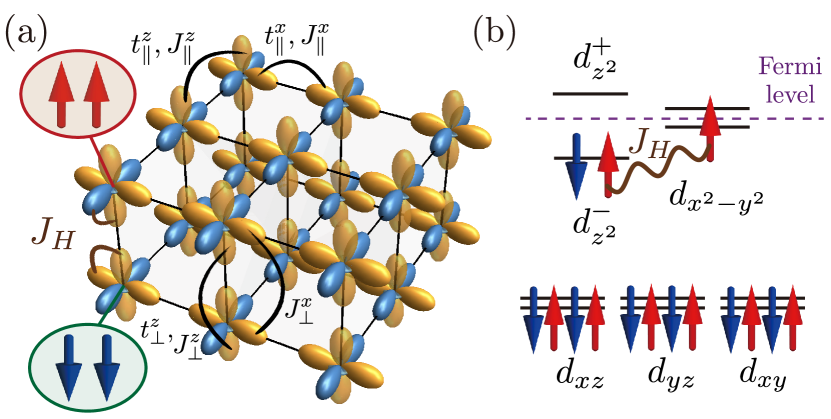
Figure 1: (a) The schematics of the bilayer two-orbital model. The various $t,J$’s are introduced for the hoppings and interactions of two orbitals on square lattices. Importantly, a strong ferromagnetic Hund coupling $J_{H}$ transmits $J^{z}_{\perp}$ of the $d_{z^{2}}$ orbital to the $d_{x^{2}-y^{2}}$ orbital, by enforcing a spin-triplet at each site (Inset). (b) The electronic configuration of two Ni^+2.5 states in one unit cell. The density per site with summing over spin is roughly $n_{1}\simeq 1/2$ and $n_{2}\simeq 1$.

Bilayer one-orbital t-J model: We first consider the limit where the $d_{2}$ orbital is Mott localized with pinned $n_{2}=1$. In this limit, $d_{2}$ orbitals form a rung-singlet insulator due to large $J_{\perp}$ and may be integrated out and one can focus on an one-orbital t-J model with the $d_{1}$ orbital. However, we emphasize that the gapped $d_{2}$ degree of freedom still plays an important role due to the Hund’s coupling. A large Hund’s coupling enforces the two orbitals to form a spin-triplet at each site. Within the restricted Hilbert space, the spins of the two orbitals align and the inter-layer spin-spin coupling $J_{\perp}^{z}$ also induces anti-ferromagnetic coupling of the $d_{1}$ orbital (see the Inset of Fig. 1(a)). Basically only the orbital symmetric part, $J^{x}_{\perp}=J^{z}_{\perp}$, can persist in the restricted Hilbert space. Consequently, we should consider a significant inter-layer $J_{\perp}$ also for the $d_{x^{2}-y^{2}}$ orbital, though there is no inter-layer hopping.

Motivated by the above considerations, we now consider an effective one-orbital t-J model for the $d_{x^{2}-y^{2}}$ orbital,

$$H_{\mathrm{eff}} =-t_{\parallel}^{x}\sum_{l,\sigma}\sum_{\langle i,j\rangle}P\left(d_{i;1;l,\sigma}^{\dagger}{\color[rgb]{0,0,0}d_{1;1;l;\sigma}}\right)P+H.c.$$

$$+J_{\parallel}^{x}\sum_{l}\sum_{\langle i,j\rangle}\vec{S}_{i;l;1}\cdot{\color[rgb]{0,0,0}\vec{S}_{j;l;1}}+J_{\perp}^{z}\sum_{i}\vec{S}_{i;t;1}\cdot\vec{S}_{i;b;1}$$ (2)

Hereafter, shorthand notation $t=t^{x}_{\parallel},J_{\parallel}=J^{x}_{\parallel}$, and $J_{\perp}=J^{z}_{\perp}$ are used, unless otherwise stated. Note that the model above is quite unconventional in the sense that we have a large $J_{\perp}$ but no inter-layer hopping $t_{\perp}$, compared to other existing models Nakata et al. (2017). This is impossible in the standard t-J model usually with $J<t$. We note a similar model (dubbed as mixed dimensional t-J model) has been proposed in the cold atom context but only out of equilibriumBohrdt et al. (2022); Hirthe et al. (2023).

We then employ the standard U(1) slave-boson mean-field theoryLee et al. (2006) and represent the electronic operator as, $d_{i;l;1;\sigma}^{\dagger}=f_{i;l;\sigma}^{\dagger}b_{i;l}$ with the constraint $n_{i;l;f}+n_{i;l;b}=1$ (see the Supplemental Material (SM) for details). In mean-field level, we decouple the following order parameters from the $J$ terms: the hopping terms $\chi_{\parallel;ij,\sigma}^{l}=2\langle f_{i;l;\sigma}^{\dagger}f_{j;l;\sigma}\rangle$, $\chi_{\perp;i;\sigma}=2\langle f_{i;t;\sigma}^{\dagger}f_{i;b;\sigma}\rangle$ and the pairing terms $\Delta_{\parallel;ij}^{l}=2s^{ij}\langle f_{i;l;\uparrow}f_{j;l;\downarrow}\rangle$, $\Delta_{\perp;i}=2\langle f_{i;t;\uparrow}f_{i;b,\downarrow}\rangle$. We obtain these order parameters from self-consistent calculations. We fix $t_{\parallel}=1$ and $J_{\parallel}=1/2$ and vary the $J_{\perp}$ and the doping $x$ in the range $0\leq x\leq 1/2$.

Here we summarize our numerical results. In the limit of small $J_{\perp}$, the model reproduces the well-known behaviors of the single-layer t-J model, with the famous $d_{x^{2}-y^{2}}$ pairing within each layer. As the strength of $J_{\perp}$ is gradually increased, there is a first-order transition after which we find s-wave pairing with dominated inter-layer pairing, as illustrated in Fig.2 (a-b). In Fig.2 (c), we find a first-order transition from the d-wave to s-wave pairing with dominated inter-layer pairing. With a large enough $J_{\perp}$ (for example, $J_{\perp}/t$>0.5), the value of $|\Delta_{\perp}|$ remains survives to the large hole doping regime with $x\simeq 0.5$.

We note that the normal Fermi surfaces are completely gapped in the s-wave pairing phase, while there are nodes in the d-wave pairing, as depicted in Fig.2 (d). $J_{\perp}/t>0.5$ is quite reasonable given that $J_{\perp}$ origins from the super-exchange of the $d_{2}$ orbital which has a large inter-layer coupling. Thus we expect an s-wave inter-layer paired superconductor in the experimental regime even with a $50\%$ hole doping. We emphasize that it is important to have large $J_{\perp}$ but with the inter-layer hopping $t_{\perp}=0$. For example, one can imagine a conventional bilayer t-J model for the $d_{z^{2}}$ orbital with $t_{\perp}>J_{\perp}$. In Fig.S1 in SM, we show that a large $t_{\perp}$ term suppresses the pairing because the hopping disfavors inter-layer spin-singlet Cooper pair. Therefore the unusual model we consider here for the $d_{x^{2}-y^{2}}$ orbital host has stronger pairing than the usual t-J model.

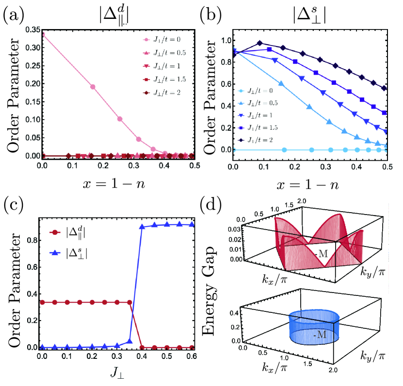
Figure 2: (a-b) Zero temperature mean-field solutions of one-orbital t-J model. We plot the filling $x$ dependence of (a) intra-layer d-wave pairing, (b) inter-layer s-wave pairing within the slave-boson framework are shown at $t_{\parallel}^{x}=1$, $J_{\parallel}^{x}=1/2$. (c) $J_{\perp}$ dependence of pairing order parameter at $x=0$. The inclusion of $J_{\perp}^{z}$ induces the first-order phase transition from $d$-wave pairing, $\Delta_{\parallel}^{d}$, to $s$-wave pairing, $\Delta_{\perp}^{s}$. (d) The energy gap of the two distinct superconducting states at the Fermi surface. Two specific cases of $J_{\perp}^{z}/t^{x}_{\parallel}=0,x=0$ (top) and $J_{\perp}^{z}/t^{x}_{\parallel}=2,x=1/2$ (bottom) are chosen for a illustration. The normal Fermi surface, centered at the M=($\pi,\pi$) point, is completely gapped with a $s$-wave pairing (bottom), while there are four point nodes with a $d$-wave pairing (top).

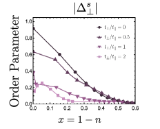
Figure 3: Mean-field order parameters of the one-orbital model. Inter-layer hopping $t_{\perp}$ dependence of the inter-layer pairing at $J_{\perp}=1/2$. The inclusion of larger inter-layer hopping $t_{\perp}$ suppressed the inter-layer pairing order parameter $\Delta_{\perp}$.

Type II t-J model: The importance of Hund’s coupling in sharing the super-exchange $J$ has been demonstrated in the simple case of $n_{2}=1$ per site. In this limit, the $d_{2}$ orbital is orbital-selective Mott localized and forms rung-singlet. Then we just ignore $d_{2}$ and deal with a one-orbital model and take the transmission of $J_{\perp}$ by hand. However, this approach is not very rigorous and needs a justification. Moreover, in real system, the $d_{2}$ orbital is likely to be slightly hole doped with $n_{2}<1$. Then the $d_{2}$ orbital should be kept in the low energy model. In this case, we need to deal with the full two-orbital model in Eq. 1. However, $U^{\prime}$ and $J_{H}$ are large and cannot be treated in perturbation or mean field level. Especially, there is no good way to capture the effect of sharing the J terms between the two orbitals from the Hund’s coupling. Apparently, a new model and a new method is called for to describe the realistic regimes with two active orbitals and a strong Hund’s coupling.

To address this challenging problem, we take a non-perturbative approach. We first take $U^{\prime},J_{H}$ to be large and project to a restricted Hilbert space. This leads to a generalization of the type II t-J model proposed by one of us in Ref.Zhang and Vishwanath, 2020. We only keep four singlon ($d^{7}$) states and three spin-triplet doublon ($d^{8}$) states. First, at each site $i$, the four singlon states can be labeled as, $\ket{a\sigma}=d^{\dagger}_{a;\sigma}\ket{G}$ where $\ket{G}$ is defined as a vacuum states where all $t_{2g}$ orbitals are fully filled with $a=1,2$ and $\sigma=\uparrow,\downarrow$. Meanwhile, the three spin-triplet doublon states are written as, $\ket{-1}=d^{\dagger}_{1\downarrow}d^{\dagger}_{2\downarrow}\ket{G}$, $\ket{0}=\frac{1}{\sqrt{2}}(d^{\dagger}_{1\uparrow}d^{\dagger}_{2\downarrow}+d^{\dagger}_{1\downarrow}d^{\dagger}_{2\uparrow})\ket{G}$ and $\ket{1}=d^{\dagger}_{1\uparrow}d^{\dagger}_{2\uparrow}\ket{G}$. Here, we ignore the site index $i$ for simplicity. The spin-singlet doubly occupied states is penalized by a large $J_{H}$ and is removed from the Hilbert space.

Now, we project the electron operator inside this $4+3=7$ dimensional Hilbert space,

$$d_{i;l;1\uparrow} =\prod_{j<i}(-1)^{n_{j}}\big{(}\ket{2\uparrow}_{il}\bra{1}_{i\l}+\frac{1}{\sqrt{2}}\ket{2\downarrow}_{il}\bra{0}_{il}\big{)},$$

$$d_{i;l;1\downarrow} =\prod_{j<i}\!(-1)^{n_{j}}\big{(}\ket{2\downarrow}_{il}\bra{-1}_{il}\!+\frac{1}{\sqrt{2}}\ket{2\uparrow}_{il}\bra{0}_{il}\big{)},$$

$$d_{i;l;2\uparrow} =-\!\prod_{j<i}\!(-1)^{n_{j}}\big{(}\ket{1\uparrow}_{il}\bra{1}_{i\;l}+\!\frac{1}{\sqrt{2}}\ket{1\downarrow}_{il}\bra{0}_{il}\big{)},$$

$$d_{i;l;2\downarrow} =-\!\prod_{j<i}(-1)^{n_{j}}\big{(}\ket{1\downarrow}_{il}\bra{-1}_{il}\!+\!\frac{1}{\sqrt{2}}\ket{1\uparrow}_{il}\bra{0}_{il}\big{)}$$ (3)

where $\prod_{j<i}(-1)^{n_{j}}$ is the Jordan-Wigner string. The spin operators for the spin-1/2 singlon state are $\vec{s}_{i;a}=\frac{1}{2}\sum_{\sigma\sigma^{\prime}}\ket{a\sigma}_{i}\vec{\sigma}_{\sigma\sigma^{\prime}}\bra{a\sigma^{\prime}}_{i}$ with $\vec{\sigma}$ as the Pauli matrices. the spin operators for the spin-one doublon states are written as $\vec{S}_{i}=\sum_{\alpha,\beta=-1,0,1}\vec{T}_{\alpha\beta]}\ket{\alpha}_{i}\bra{\beta}_{i}$. Here we have , $T_{x}=\frac{1}{\sqrt{2}}\begin{pmatrix}0&1&0\\ 1&0&1\\ 0&1&0\end{pmatrix}$ and $T_{y}=\frac{1}{\sqrt{2}}\begin{pmatrix}0&-i&0\\ i&0&-i\\ 0&i&0\end{pmatrix}$ in the $\ket{1},\ket{0},\ket{-1}$ basis.

The type II t-J model Hamiltonian is

$$H=H_{K} + J^{x}_{\parallel}\sum_{l}\sum_{\langle ij\rangle}\vec{s}_{i;l;1}\cdot\vec{s}_{j;l;1}+J^{z}_{\perp}\sum_{i}\vec{s}_{i;t;2}\cdot\vec{s}_{i;b;2}$$ (4)

$$+ J_{sd}^{\parallel}\sum_{l}\sum_{\langle ij\rangle}(\vec{s}_{i;l;1}\cdot\vec{S}_{j;l}+\cdot\vec{S}_{i;l}\cdot\vec{s}_{j;l;1})$$

$$+ J_{sd}^{\perp}\sum_{i}(\vec{s}_{i;t;2}\cdot\vec{S}_{i;b}+\vec{S}_{i;t}\cdot\vec{s}_{i;b;2})$$

$$+ J_{dd}^{\parallel}\sum_{l}\sum_{\langle ij\rangle}\vec{S}_{i;l}\cdot\vec{S}_{j;l}+J_{dd}^{\perp}\sum_{i}\vec{S}_{i;t}\cdot\vec{S}_{i;b},$$

where $H_{K}$ is the same as in Eq. 1, except that the above projected electron operators are in the $4+3=7$ Hilbert space as defined above. We have $J_{sd}^{\parallel}=\frac{1}{2}J^{x}_{\parallel}$, $J_{sd}^{\perp}=\frac{1}{2}J^{z}_{\perp}$. $J_{dd}^{\parallel}=\frac{1}{4}J^{x}_{\parallel}$ and $J_{dd}^{\perp}=\frac{1}{4}J^{z}_{\perp}$. We are interested in the filling of $n_{T}=n_{1}+n_{2}=1+n=2-x$. If the number of sites is $N_{S}$, there are $(1-x)N_{s}$ number of doublon states and $xN_{s}$ number of singlon states. The energy splitting $\Delta$ in $H_{K}$ tunes the relative density of the two orbitals. In particular, if $\Delta$ is large and positive, we only need to keep two singlon states corresponding to the $d_{2}$ orbital.

Parton mean-field theory: We employ the three-fermion parton constructionZhang and Vishwanath (2020) to deal with the type II t-J model. The four singlon states are constructed as $\ket{a\sigma}_{i}=f^{\dagger}_{i;a\sigma}\ket{0}$, while the three S=1 doublons are created by $\ket{-1}_{i}=\psi^{\dagger}_{i;1\downarrow}\psi^{\dagger}_{i;2\downarrow}\ket{0}$, $\ket{0}_{i}=\frac{1}{\sqrt{2}}(\psi^{\dagger}_{i;1\uparrow}\psi^{\dagger}_{i;2\downarrow}-\psi^{\dagger}_{i;2\uparrow}\psi^{\dagger}_{i;1\downarrow})\ket{0}$ and $\ket{1}=\psi^{\dagger}_{i;1\uparrow}\psi^{\dagger}_{i;2\uparrow}\ket{0}$. We need to impose a local constraint at each site $i$: $n_{i;f}+n_{i;\psi_{1}}=1$, $n_{i;\psi_{1}}=n_{i;\psi_{2}}$ with $n_{i;f}=\sum_{a\sigma}f^{\dagger}_{i;a\sigma}f_{i;a\sigma}$ and $n_{i;\psi_{a}}=\sum_{\sigma}\psi^{\dagger}_{i;a\sigma}\psi_{i;a\sigma}$. On average, we have $n_{f}=x$ and $n_{\psi_{1}}=n_{\psi_{2}}=1-x$ with the convention $n_{1}+n_{2}=2-x$. We introduce the notation $\Psi_{i;\sigma}=(\psi_{i;1\sigma},\psi_{i;2\sigma})^{T}$, then there is another constraint: $\Psi^{\dagger}_{i}\vec{\tau}\Psi_{i}=0$ where $\vec{\tau}$ is Pauli matrix in the color space. This constraint enforces the two colors $a=1,2$ forms singlet, thus the spin is in a triplet due to fermion statisticsZhang and Vishwanath (2020). This constraint gives a SU(2) gauge symmetry: $\Psi_{i}\rightarrow U_{i}\psi_{i}$ where $U_{i}\in SU(2)$ acting in the color space, rotating $\psi_{1}$ to $\psi_{2}$.

Within the parton construction, the projected electron operator is represented as, $d_{i;a\sigma}=\epsilon_{ab}f^{\dagger}_{i;b\sigma}\psi_{i;2\sigma}\psi_{i;1\sigma}+\frac{1}{2}\epsilon_{ab}f^{\dagger}_{i;b\bar{\sigma}}(\psi_{i;2\downarrow}\psi_{i;1\uparrow}+\psi_{i;2\uparrow}\psi_{i;1\downarrow})$. Here, $\epsilon_{ab}$ is the anti-symmetric tensor with $\epsilon_{12}=1$ and $\bar{\sigma}$ denotes the opposite spin of $\sigma$. The singlon and doublon spin operators are now represented as, $\vec{s}_{i;a}=\frac{1}{2}\sum_{\sigma,\sigma^{\prime}}f^{\dagger}_{i;a\sigma}\vec{\sigma}_{\sigma\sigma^{\prime}}f_{i;a\sigma^{\prime}}$ and $\vec{S}_{i}=\frac{1}{2}\sum_{a}\sum_{\sigma\sigma^{\prime}}\psi^{\dagger}_{i;a\sigma}\vec{\sigma}_{\sigma\sigma^{\prime}}\psi_{i;a\sigma^{\prime}}$.

Substituting all the above expressions, one can decouple the type II t-J model in Eq. 4 and perform the self-consistent mean-field calculation. We provide all details in SM. In principle, one can have a phase diagram from tuning $\Delta$ and $x$. For simplicity, we her consider the large positive $\Delta$ limit, so that $n_{2}$ is pinned to be $1$, safely ignoring $f_{1}$ and keeping only the two singlon states occupied by $f_{2\sigma}$. This corresponds to orbital selective Mott localization of the $d_{z^{2}}$ orbital and now $d_{i;2\sigma}=0$ without the $f_{1}$ operator. One important mean field decoupling is an on-site term, $\langle\psi^{\dagger}_{i;l;a\sigma}f_{i;l;2\sigma}\rangle=\frac{3}{4}\Phi_{a}$ for each spin $\sigma$ component. Due to the SU(2) gauge symmetry, we can always fix the gauge to choose $\Phi_{2}\neq 0$ while $\Phi_{1}=0$. Then $\langle\psi^{\dagger}_{i;l;2\sigma}f_{i;l;2\sigma}\rangle=3\Phi_{2}/4\neq 0$ and we have $d_{i;l;1\sigma}\sim\frac{3}{4}\Phi_{2}^{\dagger}\psi_{i;l;1\sigma}$. Now $\psi_{i;l;1\sigma}$ can be identified as the electron operator of the $d_{x^{2}-y^{2}}$ orbital with density $n_{\psi_{1}}=1-x$, while $f_{2}$ and $\psi_{2}$ hybridize and form the same band with the total density $n_{f_{2}}+n_{\psi_{2}}=1$ per site. They just represent the localized spin moments of the $d_{z^{2}}$ orbital and form a rung singlet in the bilayer model due to the large $J^{z}_{\perp}$ term.

In terms of the emergent ‘$d_{x^{2}-y^{2}}$’ orbital $\psi_{1}$, an effective model can be derived from Eq. 4 by substituting $d_{i;l_{1}\sigma}\sim\frac{3}{4}\Phi^{\dagger}_{2}\psi_{i;l;1\sigma}$,

$$H_{\psi_{1}} = \sum_{l}\sum_{\langle ij\rangle}\Big{[}-\frac{9}{16}|\Phi_{2}|^{2}t^{x}_{\parallel}\psi^{\dagger}_{i;l;1\sigma}\psi_{i;l;1\sigma}$$ (5)

$$+ J^{\parallel}_{dd}\vec{S}_{i;l;\psi_{1}}\cdot\vec{S}_{j;l;\psi_{1}}\Big{]}+J^{\perp}_{dd}\sum_{i}\vec{S}_{i;t;\psi_{1}}\cdot\vec{S}_{i;b;\psi_{1}}$$

where $\vec{S}_{i;l;\psi_{1}}=\frac{1}{2}\psi^{\dagger}_{i;l;1\sigma}\vec{\sigma}_{\sigma\sigma^{\prime}}\psi_{i;l;1\sigma^{\prime}}$ is the spin operator of $\psi_{1}$. The effective spin-spin coupling for this emergent $\psi_{1}$ orbital originates from the $J_{dd}$ coupling of the spin-one moments. As a result, the super-exchange of both $d_{z^{2}}$ and $d_{x^{2}-y^{2}}$ orbitals contribute to the $J$ coupling of this effective model. We have a large $J^{\perp}_{dd}=\frac{1}{4}J^{z}_{\perp}$ and large $J^{\parallel}_{dd}=\frac{1}{4}J^{x}_{\parallel}$ for this emergent $\psi_{1}\sim d_{1}$ orbital, even though there is no inter-layer hopping. We also note an interesting effect of reducing the hopping by a factor of $|\Phi_{2}|^{2}$ ($|\Phi_{2}|<0.5$ from our calculation as in Fig S2(c) in SM).

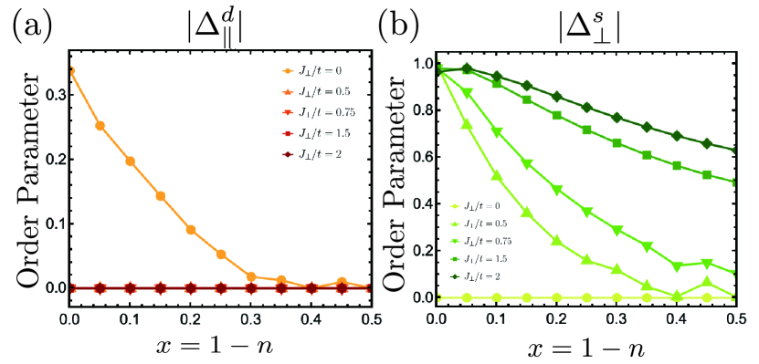
Figure 4: (a-b) Zero temperature mean-field solutions of type II t-J model in the large $\Delta$ limit. We plot the filling $x$ dependence of (a) intra-layer pairing, (b) inter-layer pairing of the emergent ‘$d_{x^{2}-y^{2}}$’ orbital at $t_{\parallel}^{x}=1$, $J_{\parallel}^{x}=1/2$. Comparing 2(a-b) and 4(a-b), we notice that the one-orbital t-J model shows similar behaviors as the more rigorous type II t-J model in the large $\Delta$ limit with the $d_{z^{2}}$ Mott localized.

We perform a full self-consistent mean field calculation involving all $f_{2},\psi_{1},\psi_{2}$ orbitals. We confirm that $f_{2},\psi_{2}$ just form a band insulator in agreement with a rung-singlet phase, while the $\psi_{1}$ orbital is at density $n_{1}=1-x$ and gets intra-layer and inter-layer pairing terms as shown in Fig. 4(a-b). Note that we still use $t$, $J_{\parallel}$, and $J_{\perp}$ as abbreviation of $t^{x}_{\parallel}$, $J^{x}_{\parallel}$ and $J^{z}_{\perp}$, and set $t=1$, $J_{\parallel}=1/2$. Varying $J_{\perp}$, we again find a first-order transition from the familiar d-wave to s-wave pairing with dominated inter-layer pairing (See Fig.S2(d)). If we take a large $J_{\perp}$ such as $J_{\perp}/t=1$, the s-wave pairing is still large at $x=0.5$. Overall, the results are qualitatively the same as the previous bilayer one-orbital t-J model (see Fig. 2(a-b)), justifying our previous treatment. However, now we achieve these results from a more precise approach of a microscopic model. The sharing of the super-exchange of one orbital to the other orbital is automatically taken care of in our model and parton framework.

Discussion: The calculation in Fig. 2 is limited to the large $\Delta$ regime with the orbital $d_{z^{2}}$ in a Mott localized state (forming a rung singlet). In the realistic system, we may have a smaller $\Delta$ and the $d_{z^{2}}$ orbital may likely be slightly doped and also participate in the pairing. This will induce some quantitative effects: (1) $d_{z^{2}}$ orbital also contributes to superconductivity; (2) The effective hole doping level of the $d_{x^{2}-y^{2}}$ can get reduced even though the total hole doping level is fixed; (3) The inter-orbital hopping may further transmit the pairing of one orbital to the other orbital. We note that a two-orbital t-J model has been proposed and studied for La₃Ni₂O₇ (for example, see Ref. Luo et al., 2023), but the previous works all ignore the important effect of sharing the super-exchange $J$ coupling between the two-orbitals by the large Hund’s coupling. We have demonstrated that this effect is crucial in the large $\Delta$ limit, so obviously it should not be ignored in the smaller $\Delta$ regime. With both orbitals active, we also can not derive a one-orbital model simply by integrating the $d_{z^{2}}$ orbital. In this regime, we believe the type II t-J model we propose here is the minimal model to capture all essential ingredients. A phase diagram of $(\Delta,x)$ can be obtained by extending our parton mean-field theory with $f_{1}$ orbital included, which we leave to future work.

We also emphasize the difference between our type II t-J model in Eq.4 and the simplified one-orbital $t-J_{\parallel}-J_{\perp}$ model in Eq.2. We here uncover the one-orbital model simply to demonstrate the essence of our mechanism of inter-layer pairing. However, we emphasize here that Eq.2 is not appropriate for Nickelate at least quantitatively even if the $d_{z^{2}}$ is Mott localized. Starting from the full model in Eq.1, one can reach Eq.2 by integrating the $d_{z^{2}}$ orbital in the $J_{H}\ll J^{z}_{\perp}$ limit and get $J_{\perp}\sim\frac{J_{H}^{2}}{J^{z}_{\perp}}$. But we believe nickelate is in the $J_{H}\gg J^{z}_{\perp}$ limit because Hund’s coupling $J_{H}$ is part of the Coulomb interaction and should be large. Then the perturbative treatment obviously breaks down and we do not see any controlled way to reach the one-orbital t-J model in Eq.2 from Eq.1 in the large $J_{H}$ regime. In the large $J_{H}$ limit, the appropriate approach is to take the large $J_{H}$ expansion instead, which leads to our type II t-J model in Eq.4 in the leading order. In the type II t-J model, the localized spin moment from $d_{z^{2}}$ orbital becomes also dynamical due to the coupling to the holes in the $d_{x^{2}-y^{2}}$ orbital. One possible effect is the polaron formation between the hole and the localized spin moment, as has already been demonstrated in a previous study of a 1D type II t-J modelZhang and Vishwanath (2022). Such polaron effect is completely ignored in the one-orbital t-J model. We believe the type II t-J model is the minimal model to capture all of the essential physics in the nickelate La₃Ni₂O₇.

Conclusion: In summary, we propose and study a bilayer type II t-J model for the superconducting La₃Ni₂O₇ under high pressure. We emphasize the important role of the Hund’s coupling between the $d_{x^{2}-y^{2}}$ and the $d_{z^{2}}$ orbital, which enforces the $d^{8}$ state to be a spin-triplet. Due to the Hund’s rule, the super-exchange of one-orbital can be shared to the other orbital. We propose a parton mean field treatment of the type II t-J model. In the limit that the $d_{z^{2}}$ is Mott localized and forms a rung singlet, we reach a bilayer one-orbital t-J model without inter-layer hopping, but with enhanced inter-layer anti-ferromagnetic spin-spin coupling $J_{\perp}$ over intra-layer hopping $t$. Mean field theory then predicts a s-wave inter-layer paired superconductor even at hole doping $50\%$, in agreement with the experiment. In future, one natural extension is to tune the orbital splitting $\Delta$ in our type II t-J model to make the $d_{z^{2}}$ orbital also slightly hole doped. We also propose future experiments to reduce $x$ through electron doping to search for an even higher $T_{c}$ than 80 K.

Note added: When finalizing the manuscript, we become aware of a preprintLu et al. (2023) which also studied a bilayer one-orbital t-J model with strong inter-layer $J_{\perp}$, which is the same as Eq.2 of our paper. However, in our opinion, the correct model in the large $J_{H}$ limit is the type II t-J model in the Eq.4 of our paper. These two models are different even when $d_{z^{2}}$ is Mott localized, see our recent paper Yang et al. (2023b) for comparisons in numerical simulations of these two models.

Acknowledgement: YHZ was supported by the National Science Foundation under Grant No. DMR-2237031.

Appendix A One-orbital t-J model and slave-boson theory

We start from the one-orbital Hamiltonian,

$$H =-t_{\parallel}^{x}\sum_{l,\sigma}\sum_{\langle i,j\rangle}P\left(d_{i;1;l,\sigma}^{\dagger}d_{1;l;\sigma}\right)P+H.c.$$

$$+J_{\parallel}^{x}\sum_{l}\sum_{\langle i,j\rangle}\vec{S}_{i;l;1}\cdot\vec{S}_{i;l;1}+J_{\perp}^{z}\sum_{i}\vec{S}_{i;t;1}\cdot\vec{S}_{i;b;1},$$ (S1)

and perform the mean field theory employing the slave boson representation, $d^{\dagger}_{i;l,1,\sigma}=f^{\dagger}_{i;l;\sigma}b_{i;l}$. Assuming $\langle b_{i}\rangle=\sqrt{x}$, after the mean-field decoupling, the mean-field Hamiltonian is given by,

$$H^{MF}_{SB} = -t_{\parallel}\sum_{l,\sigma,\langle i,j\rangle}\left(f_{i;l;\sigma}^{\dagger}f_{j;l;\sigma}+h.c.\right)-t_{\perp}\sum_{\sigma,i}\left(f^{\dagger}_{i;t;\sigma}f_{i;b;\sigma}+h.c.\right)$$

$$+D_{\parallel}\sum_{l,\langle i,j\rangle}\left(s_{ij}(f^{\dagger}_{i;l;1;\uparrow}f^{\dagger}_{j;l;1;\downarrow}-f^{\dagger}_{i;l;1;\downarrow}f^{\dagger}_{j;l;1;\uparrow})+h.c.\right)$$

$$+D_{\perp}\sum_{i}\left(f^{\dagger}_{i;t;\uparrow}f^{\dagger}_{i;b;\downarrow}-f^{\dagger}_{i;t;\downarrow}f^{\dagger}_{i;b;\uparrow}+h.c.\right),$$

with the coefficients,

$$t_{\parallel} = xt_{\parallel}^{x}+\frac{3}{8}J_{\parallel}^{x}\chi_{\parallel},\quad t_{\perp}=\frac{3}{8}J_{\perp}^{z}\chi_{\perp},$$

$$D^{\parallel} = \frac{3}{8}J^{x}_{\parallel}\Delta_{\parallel}^{d},\quad D^{\perp}=\frac{3}{8}J^{z}_{\perp}\Delta_{\perp}^{s}.$$

There are 4 mean field order parameters,

$$\chi_{\parallel} = \sum_{\sigma}\langle f^{\dagger}_{j;l;\sigma}f_{i;l;\sigma}\rangle,\quad\chi_{\perp}=\sum_{\sigma}\langle f^{\dagger}_{i;t;\sigma}f_{i;b;\sigma}\rangle,$$ (S3)

$$\Delta_{\parallel} = \langle s^{ij}(f_{i;l;\uparrow}f_{j;l;\downarrow}-f_{i;l;\downarrow}f_{j;l;\uparrow})\rangle,\quad\Delta_{\perp}=\langle f_{i;t;\uparrow}f_{j;b;\downarrow}-f_{i;t;\downarrow}f_{j;b;\uparrow}\rangle.$$ (S4)

Moreover, the chemical potential should be fixed for conserving the particle number, $n=\sum_{k,l}\langle f^{\dagger}_{k;l;\sigma}f_{k;l;\sigma}\rangle=1-x$.

Appendix B Type II t-J model and Three-fermion parton theory

We start from the type II t-J model introduced in Eq.4. Considering the large $\Delta$ limit, the singlon is formed by only $d_{2}$ orbital, thus the Hilbert space is restricted into $P_{0}=P-\ket{1,\uparrow}\bra{1,\uparrow}-\ket{1,\downarrow}\bra{1,\downarrow}$. In this Hilbert space, electron operators of $d_{2}$ orbital itself become zero, thus the kinetic Hamiltonian can be expressed in terms of $d_{1}$ orbital,

$$H = -t^{x}_{\parallel}\sum_{l,\sigma,\langle i,j\rangle}(P_{0}d^{\dagger}_{i;l;1;\sigma}d_{j;l;1;\sigma}P_{0}+h.c.)$$

$$+J^{x}_{\parallel}\sum_{l,\langle i,j\rangle}\vec{s}_{i;l;1}\cdot\vec{s}_{j;l;1}+J^{dd}_{\parallel}\sum_{l,\langle i,j\rangle}\vec{S}_{i;l}\cdot\vec{S}_{j;l}+J^{sd}_{\parallel}\sum_{l,\langle i,j\rangle}(\vec{s}_{i;l;1}\cdot\vec{S}_{j;l}+\cdot\vec{S}_{i;l}\cdot\vec{s}_{j;l;1})$$

$$+J^{z}_{\perp}\sum_{i}\vec{s}_{i;t;2}\cdot\vec{s}_{i;b;2}+J^{dd}_{\perp}\sum_{i}\vec{S}_{i;t}\cdot\vec{S}_{i;b}+J^{sd}_{\perp}\sum_{i}(\vec{s}_{i;t;2}\cdot\vec{S}_{i;b}+\vec{S}_{i;t}\cdot\vec{s}_{i;b;2})$$

Here we use the following three-fermion decomposition,

$$d_{i;l;1;\sigma}^{\dagger} = (\psi_{i;l;1;\sigma}^{\dagger}\psi_{i;l;2;\sigma}^{\dagger})f_{i;l;2;\sigma}+\frac{1}{2}(\psi_{i;l;1\uparrow}^{\dagger}\psi_{i;2;l;\downarrow}^{\dagger}+\psi_{i;1;l;\downarrow}^{\dagger}\psi_{i;2;l;\uparrow}^{\dagger})f_{i;l;2;\bar{\sigma}},$$ (S6)

$$d_{j;l;1;\sigma} = f^{\dagger}_{j;l;2;\sigma}(\psi_{j;l;2;\sigma}\psi_{j;l;1;\sigma})+\frac{1}{2}f^{\dagger}_{j;l;2;\bar{\sigma}}(\psi_{j;l;2;\downarrow}\psi_{j;l;1;\uparrow}+\psi_{j;l;2;\uparrow}\psi_{j;l;1;\downarrow}).$$ (S7)

Employing the standard decoupling principle, the mean-field Hamiltonian is given by

$$H^{MF}_{TF} = -t_{f;2}\sum_{l,\sigma,\langle i,j\rangle}\left(f_{i;l;2;\sigma}^{\dagger}f_{j;l;2;\sigma}+h.c.\right)-\sum_{a,c=1,2}t_{\psi;ac}\sum_{l,\sigma,\langle i,j\rangle}\left(\psi_{i;l;a;\sigma}^{\dagger}\psi_{j;l;c;\sigma}+h.c.\right)$$

$$-\sum_{a=1,2}C_{a}^{0}\sum_{l,\sigma,i}\left(f^{\dagger}_{i;l;2;\sigma}\psi_{i;l;a;\sigma}+\psi^{\dagger}_{i;l;a;\sigma}f_{i;l;2;\sigma}+h.c.\right)$$

$$-t_{f}^{\perp}\sum_{\sigma,i}\left(f^{\dagger}_{i;t;2;\sigma}f_{i;b;2;\sigma}+h.c.\right)-\sum_{a,c=1,2}t_{\psi;ac}^{\perp}\sum_{\sigma,i}\left(\psi^{\dagger}_{i;t;a;\sigma}\psi_{i;b;c;\sigma}+h.c.\right)$$

$$-\sum_{a=1,2}C_{a}^{\perp}\sum_{\sigma,i}\left(f^{\dagger}_{i;t;2;\sigma}\psi_{i;b;a;\sigma}+\psi^{\dagger}_{i;t;a;\sigma}f_{i;b;2;\sigma}+h.c.\right)$$

$$+D_{\psi;1}\sum_{l,\langle i,j\rangle}\left(s_{ij}(\psi^{\dagger}_{i;l;1;\uparrow}\psi^{\dagger}_{j;l;1;\downarrow}-\psi^{\dagger}_{i;l;1;\downarrow}\psi^{\dagger}_{j;l;1;\uparrow})+h.c.\right)$$

$$+D_{\psi;1}^{\perp}\sum_{i}\left(\psi^{\dagger}_{i;t;1;\uparrow}\psi^{\dagger}_{i;b;1;\downarrow}-\psi^{\dagger}_{i;t;1;\downarrow}\psi^{\dagger}_{i;b;1;\uparrow}+h.c.\right)$$

$$-\mu_{f}\sum_{l,\sigma,i}f^{\dagger}_{i;l;a;\sigma}f_{i;l;a;\sigma}-\sum_{a=1,2}\mu_{a}\sum_{l,\sigma,i}\psi^{\dagger}_{i;l;a;\sigma}\psi_{i;l;a;\sigma},$$

with the coefficients,

$$t_{\psi;11} = t_{\parallel}^{x}\left[\frac{3}{8}\chi_{f}\chi_{\psi;22}-\frac{9}{16}\Phi_{2}^{0}\Phi_{2}^{0}\right]+\frac{3}{8}J^{dd}_{\parallel}\chi_{\psi;11},$$

$$t_{\psi;22} = t_{\parallel}^{x}\left[\frac{3}{8}\chi_{f}\chi_{\psi;11}\right]+\frac{3}{8}J^{dd}_{\parallel}\chi_{\psi;22},\quad t_{f;2}=t_{\parallel}^{x}\left[\frac{3}{8}\left(\chi_{\psi;11}\chi_{\psi;22}\right)\right],\quad C_{2}^{0}=t_{\parallel}^{x}\left[-\frac{9}{8}\Phi_{2}^{0}\chi_{\psi;11}\right],$$

$$t^{\perp}_{\psi;11} = \frac{3}{8}J^{dd}_{\perp}\chi_{\psi;11},\quad t^{\perp}_{\psi;22}=\frac{3}{8}J^{dd}_{\perp}\chi_{\psi;22},\quad t_{f}^{\perp}=\frac{3}{8}J_{\perp}^{z}\chi_{f}^{\perp},\quad C_{2}^{\perp}=\frac{3}{8}J_{\perp}^{sd}\Phi_{2}^{\perp},$$

and

$$D_{\psi;1} = \frac{3}{8}J^{dd}_{\parallel}\Delta_{\psi;1},\quad D_{\psi;1}^{\perp}=\frac{3}{8}J^{dd}_{\perp}\Delta_{\psi;1}^{\perp}.$$

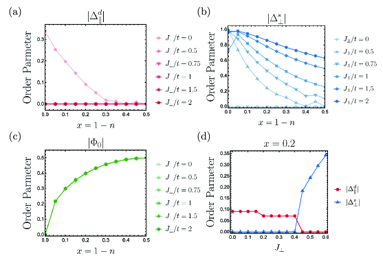
Figure S1: Mean-field order parameters of the type II t-J model at $t^{x}_{\parallel}=1$. (a-c) Doping ratio $x$ dependence of intra-layer pairing, inter-layer pairing, Kondo-like coupling at $J_{\parallel}^{x}=1/2$, (d) Inter-layer coupling $J_{\perp}$ dependence of pairings at $x=0.2$.

There are 10 mean-field order parameters in total for constructing a mean-field Hamiltonian,

$$\chi_{\psi;aa} = \sum_{\sigma}\langle\psi^{\dagger}_{j;l;a;\sigma}\psi_{i;l;a;\sigma}\rangle,\quad\chi_{f}=\sum_{\sigma}\langle f^{\dagger}_{j;l;2;\sigma}f_{i;l;2;\sigma}\rangle,\quad\Phi_{2}^{0}=\sum_{\sigma}\langle\psi^{\dagger}_{i;l;2;\sigma}f_{i;l;2;\sigma}\rangle,$$ (S9)

$$\chi^{\perp}_{\psi;aa} = \sum_{\sigma}\langle\psi^{\dagger}_{i;t;a;\sigma}\psi_{i;b;a;\sigma}\rangle,\quad\chi_{f}^{\perp}=\sum_{\sigma}\langle f^{\dagger}_{i;t;2;\sigma}f_{i;b;2;\sigma}\rangle,\quad\Phi_{2}^{\perp}=\sum_{\sigma}\langle\psi^{\dagger}_{i;t;2;\sigma}f_{i;b;2;\sigma}\rangle,$$ (S10)

$$\Delta_{\psi;1} = \langle s^{ij}(\psi_{i;l;1;\uparrow}\psi_{j;l;1;\downarrow}-\psi_{i;l;1;\downarrow}\psi_{j;l;1;\uparrow})\rangle,\quad\Delta_{\psi;1}^{\perp}=\langle\psi_{i;t;1;\uparrow}\psi_{j;b;1;\downarrow}-\psi_{i;t;1;\downarrow}\psi_{j;b;1;\uparrow}\rangle.$$ (S11)

Note that $t_{\psi;12}=C^{0}_{1}=C^{\perp}_{1}=\chi_{\psi;12}=\Phi_{1}^{0}=\Phi_{1}^{\perp}=0$, and $J_{sd}^{\parallel}=\frac{1}{2}J^{x}_{\parallel}$, $J_{sd}^{\perp}=\frac{1}{2}J^{z}_{\perp}$, $J_{dd}^{\parallel}=\frac{1}{4}J^{x}_{\parallel}$, $J_{dd}^{\perp}=\frac{1}{4}J^{z}_{\perp}$. Together with the order parameters, one should impose the constraints on the number of fermion $n_{\psi;1}=n_{\psi;1}=1-x$, and $n_{f}=x$, where the particle numbers are defined as,

$$n_{\psi;a}=\sum_{k,l}\langle\psi^{\dagger}_{k;l;a;\sigma}\psi_{k;l;a;\sigma}\rangle,\quad n_{f}=\sum_{k,l}\langle f^{\dagger}_{k;l;2;\sigma}f_{k;l;2;\sigma}\rangle.$$

In Fig.S1, we plot $(\Delta^{\parallel}_{\psi;1},\Delta^{\perp}_{\psi;1},\Phi^{0}_{2})$ upon doping with a fraction $x$ of holes. Moreover in Fig.S2, we illustrate the physical meaning of the three fermions in our parton construction. With a non-zero $\Phi=\Phi^{0}_{2}$, the $\psi_{1}$ orbital can be identified as the $d_{1}$ orbital from Eq. S7. At the same time, $\psi_{2}$,$f$ together form a localized $d_{2}$ orbital with total density $n_{i;2}+n_{i;f}=1$ per site. In our bilayer model they form a gapped rung-singlet phase.

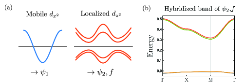
Figure S2: (a)Schematic illustrations for physical meaning of three fermions. $\psi_{1}$ itself means a $d_{1}$ orbital, while $\psi_{2}$,$f$ together form a localized $d_{2}$ orbital. (b) Energy dispersion of localized $d_{2}$ sector. We plot the dispersion of the hybridized band of $\psi_{2}$,$f$ for justifying that this sector forms a band insulator in mean field level, indicating a gapped rung-singlet phase. For an illustration, we set $J_{\perp}=1/2,x=0.1$.

References

Sun et al. (2023)H. Sun, M. Huo, X. Hu, J. Li, Z. Liu, Y. Han, L. Tang, Z. Mao, P. Yang, B. Wang, et al., Nature , 1 (2023).
Li et al. (2019)D. Li, K. Lee, B. Y. Wang, M. Osada, S. Crossley, H. R. Lee, Y. Cui, Y. Hikita, and H. Y. Hwang, Nature 572, 624 (2019).
Pan et al. (2022)G. A. Pan, D. Ferenc Segedin,
H. LaBollita, Q. Song, E. M. Nica, B. H. Goodge, A. T. Pierce, S. Doyle, S. Novakov, D. Córdova Carrizales, et al., Nature materials 21, 160 (2022).
Liu et al. (2023a)Z. Liu, M. Huo, J. Li, Q. Li, Y. Liu, Y. Dai, X. Zhou, J. Hao, Y. Lu, M. Wang, et al., arXiv preprint arXiv:2307.02950 (2023a).
Hou et al. (2023)J. Hou, P. Yang, Z. Liu, J. Li, P. Shan, L. Ma, G. Wang, N. Wang, H. Guo, J. Sun, et al., arXiv preprint arXiv:2307.09865 (2023).
Luo et al. (2023)Z. Luo, X. Hu, M. Wang, W. Wu, and D.-X. Yao, arXiv preprint arXiv:2305.15564 (2023).
Zhang et al. (2023)Y. Zhang, L.-F. Lin,
A. Moreo, and E. Dagotto, arXiv preprint arXiv:2306.03231 (2023).
Yang et al. (2023a)Q.-G. Yang, H.-Y. Liu,
D. Wang, and Q.-H. Wang, arXiv preprint arXiv:2306.03706 (2023a).
Sakakibara et al. (2023)H. Sakakibara, N. Kitamine, M. Ochi, and K. Kuroki, arXiv preprint
arXiv:2306.06039 (2023).
Gu et al. (2023)Y. Gu, C. Le, Z. Yang, X. Wu, and J. Hu, arXiv preprint arXiv:2306.07275 (2023).
Shen et al. (2023)Y. Shen, M. Qin, and G.-M. Zhang, arXiv preprint
arXiv:2306.07837 (2023).
Wú et al. (2023)W. Wú, Z. Luo,
D.-X. Yao, and M. Wang, arXiv preprint arXiv:2307.05662 (2023).
Christiansson et al. (2023)V. Christiansson, F. Petocchi, and P. Werner, arXiv
preprint arXiv:2306.07931 (2023).
Liu et al. (2023b)Y.-B. Liu, J.-W. Mei,
F. Ye, W.-Q. Chen, and F. Yang, arXiv preprint arXiv:2307.10144 (2023b).
Cao and Yang (2023)Y. Cao and Y.-f. Yang, arXiv preprint
arXiv:2307.06806 (2023).
Zhang and Vishwanath (2020)Y.-H. Zhang and A. Vishwanath, Physical Review Research 2, 023112 (2020).
Zhang and Zhu (2021)Y.-H. Zhang and Z. Zhu, Physical Review
B 103, 115101 (2021).
Zhang and Vishwanath (2022)Y.-H. Zhang and A. Vishwanath, Physical Review B 106, 045103 (2022).
Bohrdt et al. (2022)A. Bohrdt, L. Homeier,
I. Bloch, E. Demler, and F. Grusdt, Nature Physics 18, 651 (2022).
Hirthe et al. (2023)S. Hirthe, T. Chalopin,
D. Bourgund, P. Bojović, A. Bohrdt, E. Demler, F. Grusdt, I. Bloch, and T. A. Hilker, Nature 613, 463 (2023).
Lee et al. (2006)P. A. Lee, N. Nagaosa, and X.-G. Wen, Reviews of modern physics 78, 17 (2006).
Lu et al. (2023)C. Lu, Z. Pan, F. Yang, and C. Wu, “Interlayer coupling driven high-temperature superconductivity in
la3ni2o7 under pressure,” (2023), arXiv:2307.14965 [cond-mat.supr-con]
.
Yang et al. (2023b)H. Yang, H. Oh, and Y.-H. Zhang, “Strong pairing from doping-induced feshbach
resonance and second fermi liquid through doping a bilayer spin-one mott
insulator: application to la3ni2o7,” (2023b), arXiv:2309.15095 [cond-mat.str-el] .