An SU(2)-symmetric Semidefinite Programming Hierarchy for Quantum Max Cut

Abstract

Understanding and approximating extremal energy states of local Hamiltonians is a central problem in quantum physics and complexity theory. Recent work has focused on developing approximation algorithms for local Hamiltonians, and in particular the “Quantum Max Cut” (QMaxCut) problem, which is closely related to the antiferromagnetic Heisenberg model. In this work, we introduce a family of semidefinite programming (SDP) relaxations based on the Navascués-Pironio-Acín (NPA) hierarchy which is tailored for QMaxCut by taking into account its SU(2) symmetry. We show that the hierarchy converges to the optimal QMaxCut value at a finite level, which is based on a characterization of the algebra of SWAP operators. We give several analytic proofs and computational results showing exactness/inexactness of our hierarchy at the lowest level on several important families of graphs.

We also discuss relationships between SDP approaches for QMaxCut and frustration-freeness in condensed matter physics and numerically demonstrate that the SDP-solvability practically becomes an efficiently-computable generalization of frustration-freeness. Furthermore, by numerical demonstration we show the potential of SDP algorithms to perform as an approximate method to compute physical quantities and capture physical features of some Heisenberg-type statistical mechanics models even away from the frustration-free regions.

1 Introduction

The study of spin models plays a fundamental role both in physics and computer science. While most models are generally too difficult to solve exactly [Bet31, LM62, PM17], they provide insights into physical phenomena by serving as an effective description of condensed matter systems [San10, Sac23]. The antiferromagnetic Heisenberg model has been well-studied in physics and forms the focus of a recent flurry of work in optimization [GP19, PT22, AGM20, PT21], with the goal of extending the rich field of approximation algorithms to quantum problems. Already as a classical spin model, the Ising model plays a central role in the intersection between statistical physics and combinatorial optimization. The problem of computing the ground state energy for an antiferromagnetic Ising model on an arbitrary graph is known to be equivalent to the classical “Max Cut” (MaxCut) problem, one of the NP-complete problems originally listed by Karp [Kar72]. While computing the ground state energy exactly is therefore hopeless in general, the celebrated Goemans-Williamson (GW) algorithm [GW95] obtains an approximate solution which is optimal under the assumption of the Unique Games Conjecture [Kho+07] and P$\neq$NP.

The quantum Max Cut (QMaxCut) problem is closely related to the antiferromagnetic quantum Heisenberg model and plays a crucial role in understanding the hardness of approximation of Local Hamiltonian Problems. Finding the ground state of the antiferromagnetic Heisenberg model corresponds to finding the maximum energy state of QMaxCut, yet the complexity of approximating these problems likely differs. Polynomial-time approximation algorithms with constant-factor guarantees are known for QMaxCut on arbitrary interaction graphs, while these are not expected to exist for the antiferromagnetic Heisenberg model. The QMaxCut Hamiltonian was designed to bear similarity to MaxCut, and this has enabled new types of approximation algorithms for quantum local Hamiltonians that draw inspiration from classical approximations for MaxCut and other constraint satisfaction problems. QMaxCut parallels MaxCut in that the decision version of the problem is known to be QMA-complete [PM17], but unlike MaxCut the precise approximability of QMaxCut remains largely enigmatic. Recent works have been steadily improving the achievable approximation factor [GP19, PT22, AGM20, PT21, Kin22, Lee22], as well as conjecturing limitations on the achievable approximation factor [Hwa+22], but these upper and lower bounds have a sizable gap. In contrast, many combinatorial optimization problems are conjectured to be optimally approximated by techniques similar to the GW algorithm [Kho+07]. In general techniques of this form can be regarded as the first order of a family of approximation algorithms derived from the Lasserre hierarchy.

The Lasserrre hierarchy (or its dual, the Sum of Squares Hierarchy) is the tool of choice for many combinatorial optimization problems, with a well developed theory and practice (see e.g., [Lau09]). For a given problem this hierarchy corresponds to a set of semidefinite programs of increasing size and complexity (with increasing level). At high level these hierarchies converge to the optimal solution of combinatorial optimization problems under fairly general assumptions [Las01, Par03], and at low level they relax the optimization problem. The hierarchy has the benefit of providing an explicit proof that the objective achieved by the SDP bounds the optimal objective value (a “sum-of-squares” proof). On the other hand, there are known limitations on these hierarchies, with very simple objective functions provably non-convergent until the SDP reaches exponential size [Gri01].

Navascués, Pironio, and Acín (NPA) [PNA10, NPA08] generalized Lasserre’s construction [Las01] to the quantum setting, producing a powerful tool for quantum information problems. Working directly with quantum states is infeasible on classical computers since they require exponential resources in space and time in general, so in many cases NPA and similar hierarchies provide new avenues for understanding quantum systems. Such hierarchies are also referred to as noncommutative or quantum Lasserre hierarchies. Many authors have used hierarchies to characterize quantum correlations [NPA07, NPA08], design entanglement witnesses [Bac+17], and probe questions in entangled games [Kem+07, KRT09, BP15, Joh+16, Ben+18, Cui+20, Ji+22, NPA07]. In quantum Chemistry [Maz07] it is generally referred to as the variational $2$-RDM method and is used to provide computational bounds on the electronic structure problem when the dimension is too large for direct computation. More generally, SDP relaxations have been used for studying quantum many-body problems in various settings [KL21, HKR20, BP12, BH12]. Our primary application of interest is using NPA for the local Hamiltonian problem, along the lines of a recent thrust of work in quantum optimization [BH16, GP19, PT21, PT22, Hwa+22, HO22].

The main difference between NPA-like hierarchies and the Lasserre hierarchy is that NPA relaxes optimization over non-commuting rather than commuting variables. One might expect that quantum optimization landscape would parallel the classical one and that largely the same techniques would be useful for a breadth of problems, however, it appears that quantum optimization is richer in many ways. There are not known techniques which apply to many different problems, and, contrary to the classical case, it is known that the simplest “first order” algorithm is not optimal for QMaxCut [PT22], which sharply contrasts with the case for MaxCut [GW95]. Interestingly, it is unclear at this point what form the optimal algorithm should take or even if there is an optimal classical algorithm. Since QMA-hard problems have witnesses which are highly entangled, it is likely difficult to describe them and to determine what kind of quantum state/algorithm is best for the problem. Consequently, it is unclear what the best form of NPA is for QMaxCut, since NPA is defined using abstract non-commutative operators, and it could be that the optimal approximation algorithm takes advantage of a clever choice of the operators. The generic $2$-Local Hamiltonian problem generalizes many classical problems [WB03], including those which are inapproximable (with constant approximation factor) under ${\sf P}\neq{\sf NP}$ [Zuc06], so it is reasonable to expect that the optimal approximation algorithm takes advantage of the specific family or Hamiltonians it is designed for. There is precedent in this direction in that symmetry has already been used to drastically reduce the size of SDP relaxations on both the quantum [IR21] and classical [GP04] side. One immediate inconvenience of the Pauli-based NPA hierarchy used in the past [GP19, PT21a, Bra+19] is that the first level of the hierarchy fails to solve QMaxCut for the simplest types of nontrivial instances one can think of (star graphs [PT21]). This again is in sharp contrast with the classical MaxCut case, since the GW algorithm solves all of the bipartite graph instances exactly, which includes the star graphs as the simplest subclass. So far, some works have focused on an NPA hierarchy based on using the Pauli operators as variables, as well as hinted at another kind of hierarchy using the anti-ferromagnetic local terms of the Hamiltonian as non-commuting variables in the optimization [PT22].

1.1 Our Contributions

QMaxCut is the problem of solving for the largest eigenvalue of a class of instances of the $2$-Local Hamiltonian problem. QMaxCut instances are parameterized by weighted graphs. Given a vertex set $V$ and a function $w$ from pairs of vertices to $\mathbb{R}_{\geq 0}$ such a Hamiltonian is written as

$$H=\sum_{\begin{subarray}{c}i,j\in V\\ i<j\end{subarray}}w_{ij}\frac{\mathbb{I}-X_{i}X_{j}-Y_{i}Y_{j}-Z_{i}Z_{j}}{4},$$

where $\sigma_{i}$ stands for Pauli matrix $\sigma$ on qubit $i$. QMaxCut Hamiltonians are naturally invariant under conjugation by any local unitary transformation on all qubits, so Schur-Weyl duality implies that the optimal eigenstate lies in an irreducible representation of the symmetric group. Hence in defining NPA it is sensible to use permutation operators or, equivalently, polynomials in the $2$-local QMaxCut (Heisenberg) terms. We demonstrate that an abstractly defined operator program has objective matching the extremal eigenvalue and that the objective of NPA defined using this operator program converges at some finite level to the optimal solution. We learned upon completing the present work that this observation is already implicit in some results in representation theory [Pro76, Pro21, LR34]. However, a unique contribution of our work is an explicit and self-contained description of the SWAP operator program that is accessible to the broader communities such as quantum information and computer science, as well as additional context for its role in the local Hamiltonian problem. We show that the (weaker) real valued version of the NPA hierarchy agrees with the standard one at level-$1$, while giving an explicit example which we (numerically) demonstrate separates the real and complex versions in general. The real version is studied in many works [PT21, AGM20, PT22] so we motivate these works while also providing evidence that they could be improved. The lowest level of our SDP family roughly corresponds to the second lowest level of the Pauli hierarchy used in those works (one could use the lowest level of NPA with QMaxCut terms in that work instead and achieve the same approximation factor) while being smaller by an order of magnitude. Hence our results also contain an implicit run time speedup for approximating QMaxCut.

In the direction of improving existing algorithms, we give several new families of graphs where we demonstrate exactness/inexactness of our family of SDPs. In existing approximation algorithms [PT21, PT22, Kin22, Lee22] a deep understanding of instances which the low level SDP gets correct is an integral part of the analysis (the so called “star bound”), so it is possible that results established here could lead to approximation algorithms with better performance. One particularly prominent example where we demonstrate SDP exactness is for weighted star graphs. We are aware of an unpublished proof of this preceding our results [Hwa+22a], but here we provide a different proof of this fact which gives a pleasing “geometric” interpretation of monogamy of entanglement inequalities in the context of NPA hierarchies. The weighted star bound seems likely to have many applications; here we demonstrate that it implies exactness for another family of graphs, the “double star” graphs. We complement this with many other classes of graphs where we can show exactness, some of which correspond to condensed matter physics models including the Majumdar Ghosh-model and the Shastry-Sutherland model. Additionally, we provide two families (complete graphs with odd number of vertices, and “crown graphs” with certain weights) of graphs where we can analytically prove looseness of NPA at the first level. In fact we are able to provide an analytic characterization of when low levels of the hierarchy are exact on crown graphs.

Equipped with the new SDP family, we then provide extensive numerical results studying the exactness/inexactness of NPA at low levels. We first provide results for an exhaustive search among all possible unweighted graphs up to $8$ vertices, and then proceed to physically interesting cases with up to $60$ vertices. With the exhaustive search, we find no unifying features among examples where NPA is exact, and examples which are seemingly “simple” where the optimal SDP objective at low level is far from the extremal eigenvalue as well. For cycles we find that neither the first level of our SDP family or second level the hierarchy previously considered in [PT21, PT22] is exact at low levels in sharp contrast to MaxCut where the lowest level is exact on all even cycles and the second level is exact on all cycles[Bar14]. It is impossible to rigorously certify that NPA achieves the optimal eigenvalue using purely numerics, since we have many cases where the optimal SDP objective is only different from the extremal eigenvalue in the 4th or 5th decimal place. We classify graphs according to how the error of the SDP optimal solution behaves as a function of the tolerance parameter for the SDP. This lets us confidently conclude from numerics, whether the NPA is giving the exact extremal eigenvalue or not. In doing so, we are able to explicitly show separation of different NPA hierarchies, which is otherwise subtle.

Moreover, we run numerical simulations on some condensed matter physics models, demonstrating that the the lowest level of our NPA hierarchy obtains exact ground states of “frustration-free” quantum spin systems such as the Majumdar-Ghosh and Shastry-Sutherland models. We point out that this is a natural consequence from the connection between frustration-freeness and sum of squares proof, showing that the NPA hierarchy as a whole is essentially a generalization of the frustration-free notion.

The salient feature of our numerical results is that the SDP seems to predict many important physical properties even on instances where it is not achieving the optimal eigenvalue. For instance, in models with a phase transition, the SDP also appears to reflect that, by having a discontinuous optimal SDP objective as a function of the parameters. Additionally, the SDP obtains the correct decaying exponent for the correlation function as on the Heisenberg spin chain, even though there is strong evidence that it does not correctly predict the optimal energy. This suggests the capability of SDP solutions to exhibit nontrivial long-range entangled features of a critical ground state to some extent. Using “pseudo entanglement” to model quantum systems and predict their physical properties seems to be a relatively open and exciting research direction with only a few results known [Has22]. Since simulating large quantum systems is intractable on classical computers, the NPA hierarchy provides the possibility of probing features of quantum systems using (non-physical) pseudo states on a classical computer which would be unobtainable otherwise. This type of numerical analysis is only possible with our projector-based NPA hierarchy, since with the Pauli-based NPA hierarchy, the matrix size for SDP grows faster. Although the scaling difference is theoretically only a constant factor, the largest computable system size being $\sim 60$ qubits rather than $\sim 20$ makes a practical difference in terms of how deeply we can actually probe their performance. Moreover, in the projector SDP formulation, most of the variables in the moment matrix are free variables, an important feature that can significantly improve the numerical efficiency of solving SDPs when implemented in SDP solvers like MOSEK [ApS23]. This difference has enabled us to conduct both the exhaustive search and probing statistical physics model of sizes beyond what is reachable with exact diagonalization.

Note Added:

After preparing this draft we became aware of an independent group of researchers with complementary results to ours [Wat+23]. The two papers have different themes in that our paper is largely focused on understanding the performance of low level SDP relaxations for Quantum Max Cut problems, while [Wat+23] establishes a more sophisticated hierarchy and uses representation theory to analyze the extremal energies for certain Quantum Max Cut instances. There is clearly value in understanding powerful SDP relaxations, but we argue that it is also important to understand “simple” formulations because they are easier to analyze and SDPs are generally practically slow to solve. Thus there is a strong motivation to understand the simplest SDPs which offer strong bounds. We establish numerically and analytically that low levels of the hierarchy are exact on certain families of graphs with an eye toward solid state physics and approximation algorithms, while [Wat+23] is able to calculate the exact extremal eigenvalue for Hamiltonians which have a signed clique decomposition. Here the two papers are very different in that we focus on the SDP solution rather than the exact solution for the Hamiltonian problem. [Wat+23] also investigates non-commutative Groebner bases for the $SWAP$ algebra which we do not touch on and establishes finite convergence of their hierarchy at a lower level that we were able to show (Proposition 3.14 in this work versus Theorem 4.8 in [Wat+23]). We expect that both papers have much to offer one another, but we leave the full set of implications from the combined results for future work.

2 Notation

The Pauli matrices are defined as:

$$\mathbb{I}=\begin{bmatrix}1&0\\ 0&1\end{bmatrix},\,\,\,\,\,\,X=\begin{bmatrix}0&1\\ 1&0\end{bmatrix},\,\,\,\,\,\,Y=\begin{bmatrix}0&-i\\ i&0\end{bmatrix},\,\text{and}\,\,\,\,\,\,Z=\begin{bmatrix}1&0\\ 0&-1\end{bmatrix}.$$

Subscripts indicate quantum subsystems among $n$ qubits. For instance, the notation $\sigma_{i}$ is used to denote a Pauli matrix $\sigma\in\{X,Y,Z\}$ acting on qubit $i$, i.e., $\sigma_{i}:=\mathbb{I}\otimes\mathbb{I}\otimes\ldots\otimes\sigma\otimes\ldots\otimes\mathbb{I}\in\mathbb{C}^{2^{n}\times 2^{n}}$, where the $\sigma$ occurs at position $i$. $\mathbb{I}$ will also be used to denote identity matrices of arbitrary context dependent size.

We will be considering weighted graphs, $(V,\{w_{ij}\}_{ij\in V\times V})$, where each weight is non-negative. Without loss of generality we can assume the graph is complete by possibly setting some weights to zero, so we need not include an edge set in the description of the graph. The complex conjugate transpose of a given matrix will take the standard notation, $A^{*}$, and we will denote the $\max/\min$ eigenvalue of a given operator $A$ as $\mu_{max}(A)/\mu_{min}(A)$ respectively. We will be considering Hermitian operators and operators which differ from a Hermitian matrix by a similarity transform, i.e., $TAT^{-1}$ is Hermitian, so this can be well-defined by

$$\mu_{min}(A):=\min\lambda\in\mathbb{R}:\det(\lambda\mathbb{I}-A)=0;\,\,\,\,\,\,\text{and}\,\,\,\,\,\,\mu_{max}(A):=\max\lambda\in\mathbb{R}:\det(\lambda\mathbb{I}-A)=0.$$

We will have need to discuss matrix/scalar variables and will generally denote these with lower case letters, while upper case letters will be generally used to denote assignments to those variables. Polynomials in matrix variables will generally be denoted with Greek letters.

3 NPA Hierarchy

3.1 Phrasing the Local Hamiltonian problem as an Operator Program

Operator programs are a powerful and flexible way of stating difficult problems. These are generally stated as the problem of optimization over non-commuting (nc) polynomials over sets of non-commuting variables ($\{a_{i}\}$). In this context the variables $\{a_{i}\}$ are unspecified complex matrices of some finite, fixed, unspecified size ($a_{i}$ has the same size as $a_{j}$ so that multiplication is well defined). It could be the case that the objective goes to infinity as the matrices get larger or that the objective converges to some fixed value in the limit of large matrices, but for the cases we will consider here an optimal feasible solution to the problem will consist of matrices of finite size, so the programs discussed here are all well-defined and explicitly obtain their maxima/minima. Depending on the convention [PNA10], one often also includes variables $\{a_{i}^{*}\}$ for denoting the complex conjugate of the matrix variables, however, in this paper these are redundant since we will always optimize over Hermitian matrices. Polynomials in these variables will consist of linear combinations of monomials in the nc variables. The set of monomials of degree $\leq\ell$ is denoted $\Gamma_{\ell}=\{a_{i_{1}}a_{i_{2}}...a_{i_{q}}:q\leq\ell\}$ so an arbitrary degree-$\ell$ nc polynomial can be denoted $\theta(\{a_{i}\})=\sum_{\phi\in\Gamma_{\ell}}\theta_{\phi}\phi$ where $\theta_{\phi}\in\mathbb{C}$ for all $\phi$. $\Gamma_{\ell}$ will always contain a term of degree $0$, $\mathbb{I}$. $\mathbb{I}$ varies inside the program since it will have size matching the $\{a_{i}\}$ but will always denote an identity of the appropriate size.

Definition 3.1.

Given nc polynomials $\theta$ and $\{\eta_{i}\}$ with $\theta^{*}=\theta$, an operator program $\mathcal{O}$ is an optimization problem of the following form:

$$\min/\max\quad \braket{g}{\theta(\{a_{i}\})}{g}$$ (1)

$$\mathrm{s.t.}\quad \eta_{j}(\{a_{i}\})=0\,\,\text{ for all $j$},$$ (2)

$$a_{i}=a_{i}^{*},\,\forall i,$$ (3)

$$\braket{g}{g}=1.$$ (4)

To build intuition we will first consider an ncp optimization problem where the constraints force the variables to be commuting, and hence the problem reduces to a combinatorial optimization problem. Given a graph $(V,w)$, the MaxCut problem is equivalent to the following optimization problem:

$$MC(V,w):=\max\,\,\sum_{ij}w_{ij}\frac{1-z_{i}z_{j}}{2}\,\,s.t.\,\,z_{i}\in\{\pm 1\}\,\,\forall\,\,i\in[n].$$ (5)

We could also have phrased MaxCut as a local Hamiltonian problem where the local terms of the Hamiltonian are diagonal in the $Z$ basis [WB03]. In this case the largest eigenvalue would be $MC(V,w)$. Since the matrix is diagonal, the extremal eigenvector can be assumed to be a computational basis state WLOG and this basis state provides the optimal assignment for Max Cut:

$$MC(V,w)=\max\,\,\bra{g}\sum_{ij}w_{ij}\frac{\mathbb{I}-Z_{i}Z_{j}}{2}\ket{g}\,\,s.t.\,\,\braket{g}{g}=1.$$ (6)

Note that the operators above are not variables, they are the explicitly defined Pauli matrices from Section 2. Additionally the vector $\ket{g}$ is a vector variable of fixed size, unlike Definition 3.1. A natural direction for stating Eq. 6 as a ncp optimization problem is “promoting” the actual Pauli matrices $Z_{i}$ to matrix variables $z_{i}$. This would lead to a relaxation where the optimal solution to the operator program would be at least the solution to the relevant MaxCut instance. To get the objectives to match we will need to explicitly enforce constraints on $z_{i}$ which are satisfied by $Z_{i}$. We must demand that the $z_{i}$ commute, as well as that they square to the identity. The resulting operator program is

$$\max\quad \bra{g}\sum_{ij}w_{ij}\frac{\mathbb{I}-z_{i}z_{j}}{2}\ket{g}$$ (7)

$$\mathrm{s.t.}\quad z_{i}^{2}=\mathbb{I}\,\,\forall\,\,i\in[n],$$ (8)

$$z_{i}z_{j}-z_{j}z_{i}=0\,\,\forall\,\,i,j\in[n],$$ (9)

$$z_{i}^{*}=z_{i}\,\,\forall\,\,i\in[n],$$ (10)

$$\braket{g}{g}=1.$$ (11)

Proposition 3.2.

The program defined in Eq. 7 has optimal objective $MC(V,w)$.

Proof.

Let $z_{i}=Z_{i}^{\prime}$ and $\ket{g}=\ket{\psi}$ be the optimal solution to Eq. 7. $Z_{i}^{\prime}$ all square to the identity and are Hermitian so they have at most two eigenvalues, $\{\pm 1\}$. Since the $Z_{i}^{\prime}$ all commute we can construct a basis which simultaneously diagonalizes all the $Z_{i}^{\prime}$. The objective is diagonal in this basis so we may assume WLOG that $\ket{\psi}$ is one of these basis elements and that $\bra{\psi}Z_{i}^{\prime}\ket{\psi}\in\{\pm 1\}$. Let us define $z_{i}^{\prime}=\bra{\psi}Z_{i}^{\prime}\ket{\psi}\in\{\pm 1\}$, so $(z_{i}^{\prime})^{2}=1$. By the eigenvector property,

$$\bra{\psi}\sum_{ij}w_{ij}\frac{\mathbb{I}-Z_{i}^{\prime}Z_{j}^{\prime}}{2}\ket{\psi}=\sum_{ij}w_{ij}\frac{1-\bra{\psi}Z_{i}^{\prime}\ket{\psi}\bra{\psi}Z_{j}^{\prime}\ket{\psi}}{2}=\sum_{ij}w_{ij}\frac{1-z_{i}^{\prime}z_{j}^{\prime}}{2},$$

so the optimal objective of Eq. 7 is less than or equal to $MC(V,w)$. We already know that optimal objective of Eq. 7 is greater than or equal to $MC(V,w)$ since it is a relaxation.

∎

Naturally we may consider a generic $2$-Local Hamiltonian problem and ask similar questions. Arbitrary $2$-Local Hamiltonians may be written as $H=\sum_{ij}H_{ij}$ where $H_{ij}$ acts only on qubits $i$ and $j$. We can express each $H_{ij}$ in the Pauli basis as

$$H_{ij}=\sum_{\sigma,\gamma\in\{\mathbb{I},X,Y,Z\}}c_{\sigma,\gamma}^{ij}\,\,\sigma_{i}\gamma_{j},$$ (12)

for $c_{\sigma,\gamma}^{ij}\in\mathbb{R}$. This lets us express the overall Hamiltonian as

$$H=\sum_{ij}\sum_{\sigma,\gamma\in\{\mathbb{I},X,Y,Z\}}c_{\sigma,\gamma}^{ij}\,\,\sigma_{i}\gamma_{j}.$$ (13)

The maximum eigenvalue problem is then

$$\mu_{max}(H)=\max\,\,\bra{g}\sum_{ij}\sum_{\sigma,\gamma\in\{\mathbb{I},X,Y,Z\}}c_{\sigma,\gamma}^{ij}\,\,\sigma_{i}\gamma_{j}\ket{g}\,\,s.t.\,\,\braket{g}{g}=1.$$ (14)

We may promote the Pauli matrices above to operator variables, $X_{i}\rightarrow x_{i},Y_{i}\rightarrow y_{i},Z_{i}\rightarrow z_{i}$, to get a relaxation, but we will need to know what constraints to enforce to ensure that the operator problem has the same objective as the explicit local Hamiltonian problem we have in mind, just as for MaxCut. Enforcing constraints of the form Eqs. 8, 9 and 10 plus additional anti-commutation constraints is sufficient:

Definition 3.3.

Given a $2$-Local Hamiltonian $H$ on $n$ qubits,

$$\mathcal{Pauli}(H):=\max\quad \bra{g}\left(\sum_{ij}\sum_{\sigma,\gamma\in\{\mathbb{I},x,y,z\}}c_{\sigma,\gamma}^{ij}\,\,\sigma_{i}\gamma_{i}\right)\ket{g}$$ (15)

$$\mathrm{s.t.}\quad \text{for all distinct $j,k\in[n]$}:$$

$$\mathbb{I}=x_{j}^{2}=y_{j}^{2}=z_{j}^{2},$$ (16)

$$\{x_{j},y_{j}\}=0,\,\,\{x_{j},z_{j}\}=0,\,\,\{y_{j},z_{j}\}=0,$$ (17)

$$a_{j}b_{k}-b_{k}a_{j}=0\,\,\forall\,\,a,b\in\{x,y,z\},$$ (18)

$$x_{j}^{*}=x_{j},\,\,y_{j}^{*}=y_{j},\,\,z_{j}^{*}=z_{j},$$ (19)

$$\braket{g}{g}=1.$$ (20)

Proposition 3.4 (Theorem 2.3 in [Cha+17]).

$\mu_{max}(H)=\mathcal{Pauli}(H)$.

The proof of this statement proceeds by showing that any operators which satisfy the relations above must be equal to the Pauli matrices up to overall unitary and tensoring with identity matrices. In a sense the smallest feasible solution to $\mathcal{Pauli}(H)$ are the Pauli matrices themselves and larger solutions must have the same objective. In the language of representation theory, the Pauli group has only two irreducible representations: the trivial representation and the defining representation.

3.2 QMaxCut as an Operator Program

While the $\mathcal{Pauli}$ program is very nice because of its generality, Hamiltonians are often best studied with the natural symmetry present taken into account. Our interest is in a specific family of Local Hamiltonians known as “Quantum Max Cut” (QMaxCut) in many works [GP19, PT22, AGM20, PT21], so our aim is to produce the “natural” operator programs for these Hamiltonians. Given a weighted graph $(V,w)$ with non-negative weights $w_{ij}\geq 0$, the corresponding QMaxCut instance is defined on $n=|V|$ qubits by

$$QMC(V,w):=\mu_{max}\left(\sum_{ij}w_{ij}H_{ij}\right),$$ (21)

where $H_{ij}:=\frac{1}{4}\left(\mathbb{I}-X_{i}X_{j}-Y_{i}Y_{j}-Z_{i}Z_{j}\right)$. The term $H_{ij}$ is a projector to the singlet state $|\psi^{-}_{ij}\rangle:=(|0_{i}1_{j}\rangle-|1_{i}0_{j}\rangle)/\sqrt{2}$. Note that the singlet state is order sensitive ($|\psi^{-}_{ij}\rangle=-|\psi^{-}_{ji}\rangle$), but the Hamiltonian is not ($H_{ij}=H_{ji}$). This Hamiltonian has been well-studied in physics for decades, serving as central model for quantum magnetism. It has the nice property that it is rotation-invariant; that is, for any single-qubit unitary $U$, we have $(U^{\dagger})^{\otimes n}H_{ij}U^{\otimes n}=H_{ij}$. $H\succeq 0$ since we only consider non-negative weights $w$ ($\succeq 0$ denotes that a matrix is positive semidefinite.).

It will be convenient for us to have a definition of another Hamiltonian which is simply an affine shift of the QMaxCut Hamiltonian. If we define the usual quantum SWAP operators as

$$P_{ij}=\begin{bmatrix}1&0&0&0\\ 0&0&1&0\\ 0&1&0&0\\ 0&0&0&1\end{bmatrix}_{ij}=\frac{\mathbb{I}+X_{i}X_{j}+Y_{i}Y_{j}+Z_{i}Z_{j}}{2},$$ (22)

we can then define

$$SWAP(V,w)=\mu_{min}\left(\sum_{ij\in E}w_{ij}P_{ij}\right).$$ (23)

The extremal eigenvalues are related as:

$$SWAP(V,w)=\sum_{jk}w_{jk}-2QMC(V,w).$$ (24)

Our approach is to promote the operators $H_{ij}$ and $P_{ij}$ to variables, but we are left with the same question of deciding what constraints to include to accurately capture the local Hamiltonian problem. Our work naturally extends that of  [PT22], who used such operators to obtain an optimal approximation for QMaxCut using product states. The following sets of constraints are sufficient for QMaxCut and SWAP Hamiltonians respectively:

Definition 3.5 ($\mathcal{Proj}(V,w)$).

Given Hamiltonian $H=\sum_{ij}w_{ij}H_{ij}$ corresponding to graph $(V,w)$, define

$$\mathcal{Proj}(H)=\mathcal{Proj}(V,w):=\max\quad \bra{g}\left(\sum_{jk}w_{jk}h_{jk}\right)\ket{g}$$ (25)

$$\mathrm{s.t.}\quad \forall\text{ distinct }\,\,i,j,k,l\in[n]:$$

$$h_{ij}^{2}=h_{ij},$$ (26)

$$h_{ij}h_{kl}=h_{kl}h_{ij},$$ (27)

$$h_{ij}h_{jk}+h_{jk}h_{ij}=\frac{1}{2}(h_{ij}+h_{jk}-h_{ik}),$$ (28)

$$h_{ij}^{*}=h_{ij},$$ (29)

$$\braket{g}{g}=1.$$ (30)

Definition 3.6 ($\mathcal{Perm}(V,w)$).

Given Hamiltonian $H=\sum_{ij}w_{ij}P_{ij}$ corresponding to graph $(V,w)$, define

$$\mathcal{Perm}(H)=\mathcal{Perm}(V,w):=\min\quad \bra{g}\left(\sum_{jk}w_{jk}p_{jk}\right)\ket{g}$$ (31)

$$\mathrm{s.t.}\quad \forall\text{ distinct }\,\,i,j,k,l\in[n]:$$

$$p_{ij}^{2}=\mathbb{I},$$ (32)

$$p_{ij}p_{kl}=p_{kl}p_{ij},$$ (33)

$$p_{ij}p_{jk}+p_{jk}p_{ij}=p_{ij}+p_{jk}+p_{ik}-\mathbb{I},$$ (34)

$$p_{ij}^{*}=p_{ij},$$ (35)

$$\braket{g}{g}=1.$$ (36)

It is easy to verify that $\mathcal{Proj}$ and $\mathcal{Perm}$ are equivalent in the sense that optimal objectives of $\mathcal{Perm}$ and $\mathcal{Proj}$ are affine shifts of one another:

$$\mathcal{Perm}(V,w)=\sum_{jk\in E}w_{jk}-2\mathcal{Proj}(V,w).$$ (37)

This can be verified by observing that if $\{P_{jk}^{\prime}\}$ is a feasible solution for $\mathcal{Perm}$ then $\{(\mathbb{I}-P_{jk}^{\prime})/2\}$ is a feasible solution for $\mathcal{Proj}$ and that if $\{H_{jk}^{\prime}\}$ is feasible for $\mathcal{Proj}$ then $\{\mathbb{I}-2H_{jk}^{\prime}\}$ is feasible for $\mathcal{Perm}$.

The intuition behind the $\mathcal{Perm}$ constraints can most easily be understood in the context of the representation theory of the symmetric group. It is well known that the symmetric group has a “finite presentation”. Loosely speaking this means that there is a finite set of generators such that any element of the symmetric group can be written as the product of generators, and any product of elements from the symmetric group can be inferred from some finite set of multiplication rules on those generators. Using standard notation, the symmetric group $S_{n}$ is generated by transpositions $(i,j)$ subject to the following rules:

$$\forall\text{ distinct }\,\,i,j,k,l\in[n]:$$

$$(i,j)^{2} =1,$$ (38)

$$(i,j)(k,l) =(k,l)(i,j),$$ (39)

$$(i,j)(j,k)(i,j) =(j,k)(i,j)(j,k).$$ (40)

Since all multiplicative identities can be derived from these rules, if we have operators $p_{ij}$ which satisfy analogous relations then multiplication of products of monomials in $\{p_{ij}\}$ must behave exactly like products of transpositions. Hence feasible solutions $\{p_{ij}^{\prime}\}$ must correspond to a representation of the symmetric group (see Appendix A.1). Note that there is a correspondence between Eq. 32 and Eq. 38 as well as between Eq. 33 and Eq. 39, but apparently none for Eq. 40. Instead, the operator program $\mathcal{Perm}$ contains an additional “anti-commuting constraint” Eq. 34. $\mathcal{Perm}$ actually has an implicit constraint corresponding to Eq. 40 (Proposition 3.7), so the constraints present enforce that the operators $p_{ij}$ “look like” a finite presentation of the symmetric group, plus an additional anti-commuting constraint. This fact is crucial for understanding why the operator programs listed are accurately capturing the relevant local Hamiltonian problems (Theorem 3.8). Equations 32, 33, 34 and 35 force the operators to correspond to a representation of the Symmetric group, and Eq. 34 further forces the operators to correspond to the correct representation for the Hamiltonian.

Proposition 3.7.

For all distinct $i,j,k\in[n]$, $\mathcal{Perm}$ satisfies the additional constraint

$$p_{ij}p_{jk}p_{ij}=p_{ik},$$ (41)

and $\mathcal{Proj}$ satisfies the additional constraint

$$4h_{ij}h_{jk}h_{ij}=h_{ij}.$$ (42)

Proof.

From the anticommutation relation Eq. 28, we can expand $h_{jk}=h_{ij}+h_{ik}-2(h_{ij}h_{ik}+h_{ik}h_{ij})$ to obtain

$$h_{ij}h_{jk}h_{ij} = h_{ij}\bigl{(}h_{ij}+h_{ik}-2(h_{ij}h_{ik}+h_{ik}h_{ij})\bigr{)}h_{ij}$$ (43)

$$= h_{ij}-3h_{ij}h_{ik}h_{ij},$$ (44)

where we used Eq. 30 as well. Repeating the same substitution for $h_{ik}$ in the second term gives $h_{ij}h_{jk}h_{ij}=h_{ij}-3\bigl{(}h_{ij}-3h_{ij}h_{jk}h_{ij}\bigr{)}$, which results in Eq. 42 after solving the linear equation. To obtain Eq. 41, apply the same proof with $h_{ij}=(\mathbb{I}-p_{ij})/2$. ∎

This additional constraint Eq. 42 is actually one of the basic relations in the Temperley-Lieb algebra [TL71] describing the 1-dimensional Heisenberg chain and variants. The factor of 4 could be understood in relation with other algebraic structures used for analyzing the Heisenberg model [San05, BS06]. Furthermore, an immediate corollary of Proposition 3.7 is that

$$p_{ij}p_{jk}p_{ij}=p_{ik}=p_{jk}p_{ij}p_{jk},$$ (45)

giving the constraint corresponding to Eq. 40. Reasoning as above one can obtain:

Theorem 3.8 ([Pro76]).

$\mathcal{Perm}(V,w)=SWAP(V,w)$.

Proof.

See Section A.3. ∎

Corollary 3.9.

$\mathcal{Perm}$ is a QMA-complete operator program.

Proof.

Determining $SWAP(G,w)$ is QMA-complete [PM17] and by Theorem 3.8 finding $SWAP(G,w)$ is equivalent to finding $\mathcal{Perm}(G,w)$. ∎

Theorem 3.8 establishes that the optimal operator variables in $\mathcal{Perm}$ and actual quantum operators in $SWAP$ are the same, or that $\mathcal{Perm}$ can be optimized using the fixed assignments $p_{ij}=P_{ij}$ WLOG. Similarly, the abstract operator variables in $\mathcal{Proj}$ denoted by $h_{ij}$ become indistinguishable from the actual quantum operators of QMaxCut denoted by $H_{ij}$ when they are optimized according to the program. This is somewhat surprising, since in general, there are infinite amount of nontrivial relations between singlet projectors $H_{ij}$ that include higher order terms. The theorem implies that all of them must be derivable purely from relations in the program, namely Eqs. 26 to 29 for $h_{ij}$, and Eqs. 32 to 35 for $p_{ij}$. Proposition 3.7 could be seen as one such derivation, and we show other examples in Appendix B. Later in section 4, we will take advantage of this equivalence, and identify $h_{ij}$ and $H_{ij}$ for practical purposes. If we explicitly add the constraints Eq. 45 to the program then the above conclusions hold even if only a single anti-commuting constraint is included. So if we only enforced $p_{12}p_{23}+p_{23}p_{12}=p_{12}+p_{23}+p_{13}-\mathbb{I}$ and did not include any other anti-commuting constraints then we would still have $SWAP(V,w)=\mathcal{Perm}(V,w)$, essentially because a single constraint rules out all the incorrect representations.

3.3 The Hierarchy

The NPA hierarchy [PNA10] gives a general procedure for constructing a family of semidefinite optimization programs parameterized by “level” which provide increasingly accurate relaxations on operator programs $\mathcal{O}$ (Definition 3.1). The definition given in [PNA10] is more general than the one presented here which we have simplified for our particular application. We motivate the definition of the hierarchy by considering a “moment matrix”. Let $\{A_{i}\}$, $\ket{G}$ be some feasible solution to $\mathcal{O}$. $M_{\ell}$ is defined to be a complex Hermitian matrix with rows/columns indexed by elements of $\Gamma_{\ell}:=\{a_{i_{1}}a_{i_{2}}...a_{i_{m}}:m\leq\ell\}$, the set of monomials of degree $\leq\ell$. Entries of $M_{\ell}$ are defined so that

$$M_{\ell}(a_{i_{1}}...a_{i_{m}},a_{j_{1}}...a_{j_{r}}) :=\braket{G}{(A_{i_{1}}...A_{i_{m}})^{*}A_{j_{1}}...A_{j_{r}}}{G}$$ (46)

$$=\braket{G}{A_{i_{m}}...A_{i_{1}}A_{j_{1}}...A_{j_{r}}}{G}.$$

By definition $M_{\ell}$ gives consistent values for all monomials in $\Gamma_{2\ell}$, and we can unambiguously define

$$M_{\ell}(a_{i_{1}}...a_{i_{r}}):=\begin{cases}M_{\ell}(\mathbb{I},a_{i_{1}}...a_{i_{r}})\text{ if $r\leq\ell$},\\ M_{\ell}(a_{i_{\ell}}...a_{i_{1}},a_{i_{\ell+1}}...a_{i_{r}})\text{ otherwise}.\end{cases}$$ (47)

Similarly for any degree-$\ell$ nc polynomials $\beta(\{A_{i}\})=\sum_{\phi\in\Gamma_{\ell}}\beta_{\phi}\phi(\{A_{i}\})$ and $\gamma(\{A_{i}\})=\sum_{\phi\in\Gamma_{\ell}}\gamma_{\phi}\phi(\{A_{i}\})$, with $\beta_{\phi},\gamma_{\phi}\in\mathbb{C}$ for all $\phi$, we define

$$M_{\ell}(\beta,\gamma):=\sum_{\phi,\phi^{\prime}\in\Gamma_{\ell}}{\beta_{\phi}}^{*}\gamma_{\phi^{\prime}}\braket{G}{\phi^{*}(\{A_{i}\})\phi^{\prime}(\{A_{i}\})}{G}=\sum_{\phi,\phi^{\prime}\in\Gamma_{\ell}}{\beta_{\phi}}^{*}\gamma_{\phi^{\prime}}M_{\ell}(\phi,\phi^{\prime})=\sum_{\phi,\phi^{\prime}\in\Gamma_{\ell}}(\beta_{\phi})^{*}\gamma_{\phi^{\prime}}M_{\ell}(\phi^{*}\phi^{\prime}).$$ (48)

Furthermore, since the polynomials $\{\eta_{k}\}$ corresponding to the constraints must evaluate to zero for the variables $\{A_{i}\}$, we must also have that $0=\eta_{k}(\{A_{i}\})=\bra{G}\eta_{k}(\{A_{i}\})\ket{G}=M_{\ell}(\eta_{k})$. More generally, feasibility for $\mathcal{O}$ implies that for any nc polynomials $\beta,\gamma$ with $\deg(\beta\eta_{k}\gamma)\leq 2\ell$,

$$M_{\ell}(\beta\eta_{k}\gamma)=0,$$ (49)

since $\bra{G}\beta\eta_{k}\gamma\ket{G}=\bra{G}\beta 0\gamma\ket{G}$. The matrix $M_{\ell}$ also naturally satisfies

$$M_{\ell}=M_{\ell}^{*}\text{ ~{}~{}~{}and~{}~{}~{} }M_{\ell}\succeq 0,$$ (50)

where the latter constraint can be seen from the fact that for any complex column vector $v$, $v^{*}M_{\ell}v=M_{\ell}(\beta,\beta)=\bra{G}\beta^{*}\beta\ket{G}\geq 0$ for some $\beta$ that is a degree-$\ell$ nc polynomial.

Given an operator program $\mathcal{O}$, the $\ell$-th level of the NPA hierarchy, denoted by $NPA_{\ell}(\mathcal{O})$, is the optimization of the matrix $M_{\ell}$ as a variable, subject to the above properties viewed as constraints, not requiring a corresponding legitimate vector $\ket{G}$ or operators $\{A_{i}\}$. $NPA_{\ell}(\mathcal{O})$ relaxes $\mathcal{O}$ since we could have used the optimal $\ket{G},\{A_{i}\}$ to define $M_{\ell}$, so if $\mathcal{O}$ is a maximization problem, $NPA_{\ell}(\mathcal{O})\geq\mathcal{O}$. For a given monomial $a_{i_{1}}...a_{i_{r}}$, $M_{\ell}(a_{i_{1}}...a_{i_{r}})$ is defined as a specific entry of $M_{\ell}$ according to Eq. 47. However, there are many other distinct entries of $M_{\ell}$ which will match. For example, $M_{2}(a_{1}a_{2}):=M_{2}(\mathbb{I},a_{1}a_{2})$, but $M_{2}(\mathbb{I},a_{1}a_{2})=M_{2}(a_{1},a_{2})=M_{2}(a_{2}a_{1},\mathbb{I})$. In $NPA_{\ell}$ we will force the value of $M_{\ell}(a_{i_{1}}...a_{i_{r}})$ to be consistent with the other distinct entries by enforcing that these other entries of $M_{\ell}$ are equal to the “cannonical” value $M_{2}(a_{1}a_{2}):=M_{2}(\mathbb{I},a_{1}a_{2})$. Note that $M_{\ell}$ will be indexed by variables $\phi\in\Gamma_{\ell}$ of the original operator program, but these $\phi$ do not vary inside $NPA_{\ell}$.

Definition 3.10 ($NPA_{\ell}(\mathcal{O})$).

Given an operator program $\mathcal{O}$ with objective to max / min the extremal eigenvalue of a nc polynomial $\theta\in\text{span}(\Gamma_{2\ell})$ satisfying $\theta^{*}=\theta$ and subject to constraints $\{\eta_{k}\}$, define

$$NPA_{\ell}(\mathcal{O}):=\max/\min\quad M_{\ell}(\theta)$$ (51)

$$\mathrm{s.t.}\quad M_{\ell}(\mathbb{I})=1,$$ (52)

$$M_{\ell}(\phi,\phi^{\prime})=M_{\ell}(\phi^{*}\phi^{\prime})~{}~{}~{}~{}\forall\phi,\phi^{\prime}\in\Gamma_{\ell},$$ (53)

$$M_{\ell}(\beta\eta_{k}\gamma)=0~{}~{}~{}~{}\forall\beta,\gamma\in\Gamma_{2\ell},\eta_{k}:\deg(\beta\eta_{k}\gamma)\leq 2\ell,$$ (54)

$$M_{\ell}\succeq 0,~{}\mathrm{Hermitian}.$$ (55)

In several works [PT21, AGM20, PT22] a “real version” of $NPA_{\ell}$ is studied, $NPA_{\ell}^{\mathbb{R}}$. The key difference is that $NPA_{\ell}^{\mathbb{R}}$ takes only the real portion of the moment matrix, effectively “zeroing out” skew-Hermitian polynomials.

Definition 3.11 ($NPA_{\ell}^{\mathbb{R}}(\mathcal{O})$).

Given an operator program $\mathcal{O}$ with objective to max / min the extremal eigenvalue of a nc polynomial $\theta\in\text{span}(\Gamma_{2\ell})$ satsifying $\theta^{*}=\theta$ and subject to constraints $\{\eta_{k}\}$, define

$$NPA_{\ell}^{\mathbb{R}}(\mathcal{O}):=\max/\min\quad M_{\ell}^{\mathbb{R}}(\theta)$$ (56)

$$\mathrm{s.t.}\quad M_{\ell}^{\mathbb{R}}(\mathbb{I})=1,$$ (57)

$$M_{\ell}^{\mathbb{R}}(\phi,\phi^{\prime})=M_{\ell}^{\mathbb{R}}(\phi^{*}\phi^{\prime})~{}~{}~{}~{}\forall\phi,\phi^{\prime}\in\Gamma_{\ell},$$ (58)

$$M_{\ell}^{\mathbb{R}}((\beta\eta_{k}\gamma+\gamma^{*}\eta_{k}^{*}\beta^{*})/2)=0~{}~{}~{}~{}\forall\beta,\gamma\in\Gamma_{2\ell},\eta_{k}:\deg(\beta\eta_{k}\gamma)\leq 2\ell,$$ (59)

$$M_{\ell}^{\mathbb{R}}\succeq 0,~{}\mathrm{Symmetric}.$$ (60)

As noted in other works [Bra+19, GP19], $NPA_{\ell}^{\mathbb{R}}(\mathcal{O})$ is a relaxation on $NPA_{\ell}(\mathcal{O})$ ($NPA_{\ell}(\mathcal{O})\leq NPA_{\ell}^{\mathbb{R}}(\mathcal{O})$ if $\mathcal{O}$ is a maximization problem) since given a feasible $M_{\ell}$ for $NPA_{\ell}(\mathcal{O})$, we can take $M_{\ell}^{\mathbb{R}}:=(M_{\ell}+(M_{\ell}^{*})^{T})/2$ to obtain a feasible solution to $NPA_{\ell}^{\mathbb{R}}$ with the same objective, but not necessarily the other way around. We show explicit examples in Section 5.1.2 where the separation is strict for the $\mathcal{Pauli}$ case. However, for the specific SDP we focus on most in this paper, $NPA_{1}(\mathcal{Proj})$, this is a distinction without a difference:

Proposition 3.12.

For any weighted graph $(V,w)$, $NPA_{1}(\mathcal{Proj}(V,w))=NPA_{1}^{\mathbb{R}}(\mathcal{Proj}(V,w))$.

Proof.

Let $M_{1}^{\mathbb{R}}$ be a feasible solution to $NPA_{1}^{\mathbb{R}}(\mathcal{Proj})$. We claim that $M_{1}^{\mathbb{R}}$ is feasible for $NPA_{1}(\mathcal{Proj})$ and hence $NPA_{1}^{\mathbb{R}}(\mathcal{Proj})\leq NPA_{1}(\mathcal{Proj})$. This is demonstrated by showing that all the constraints $\eta$ enforced on $M_{1}^{\mathbb{R}}$ (constraints of the form Equation 59) are Hermitian and hence $M_{1}^{\mathbb{R}}(\eta+\eta^{*})=0$ implies $M_{1}^{\mathbb{R}}(\eta)=0$. It is easy to see that the nc polynomials $\eta$ of the form $h_{ij}^{2}-h_{ij}$ and $h_{ij}h_{jk}+h_{jk}h_{ij}-(h_{ij}+h_{jk}-h_{ik})/2$ are Hermitian, hence $M_{1}^{\mathbb{R}}(\eta)=0$ for these polynomials. Since we are looking at moment matrices with a maximum degree $2$ if $\beta\eta\gamma$ has max degree $2$ for $\eta$ one of the polynomials above $\beta=\mathbb{I}=\gamma$ so there are no other constraints to check and $M_{1}^{\mathbb{R}}$ must be feasible for $NPA_{1}(\mathcal{Proj})$

∎

Each $NPA_{\ell}$ can be solved via semidefinite programming, and the dual set of programs is called the Sum of Squares (SoS) hierarchy due to the interpretation of the hierarchy as an optimization over sum of squares proofs. To motivate this imagine we are trying to maximize an nc polynomial $\theta$ and obtain an expression of the form

$$\lambda\mathbb{I}-\theta=\sum_{i}\psi_{i}^{*}\psi_{i}+\sum_{j}\beta_{j}\eta_{j}\gamma_{j},$$ (61)

where $\lambda\in\mathbb{R}$, $\psi_{i}\in\mathrm{span}_{\mathbb{C}}(\Gamma_{\ell})$ for all $i$ and $\deg(\beta_{j}\eta_{j}\gamma_{j})\leq 2\ell$ for all $j$. Since $\eta_{k}$ are constraints of $\mathcal{O}$ we must have that

$$\lambda\mathbb{I}-\theta=\sum_{i}\psi_{i}^{*}\psi_{i}$$ (62)

for any feasible solution to $\mathcal{O}$. $\sum_{i}\psi^{*}\psi_{i}$ is manifestly $\succeq 0$ so for all feasible solutions $\bra{G}\lambda\mathbb{I}-\theta\ket{G}\geq 0\Rightarrow\lambda\geq\bra{G}\theta\ket{G}$ which implies $\lambda\geq NPA_{\ell}(\mathcal{O})$. An expression of the form Eq. 61 is generally referred to as a sum of squares proof. The SoS optimization problem at level $\ell$ is to find the smallest $\lambda$ such that $\lambda\mathbb{I}-\theta$ can be deformed via the constraints to an expression of the form $\sum_{i}\psi^{*}\psi$: $\lambda\mathbb{I}-\theta-\sum_{j}\beta_{j}\eta_{j}\gamma_{j}=\sum_{i}\psi_{i}^{*}\psi_{i}$. Crucially, the constraints that the SoS proof uses are of degree at most $\ell$ at the corresponding level ($\deg(\beta_{j}\eta_{j}\gamma_{j})\leq 2\ell$). For ease of reference, define the set of constraint deformation polynomials as

$$U^{\ell}(\{\eta_{k}\}):=\mathrm{span}_{\mathbb{C}}\{\beta\eta_{k}\gamma:\beta,\gamma\in\Gamma_{\ell},\deg(\beta\eta_{k}\gamma)\leq 2\ell\}$$ (63)

Definition 3.13 ($SoS_{\ell}(\mathcal{O})$).

Given an operator program $\mathcal{O}$ with objective to max/min the extremal eigenvalue of $\theta$ subject to the constraints $\{\eta_{k}\}$,

$$SoS_{\ell}(\mathcal{O}):=\min/\max\quad \lambda$$ (64)

$$\mathrm{s.t.}\quad \sum_{i}\psi_{i}^{*}\psi_{i}+\beta=\begin{cases}\lambda\mathbb{I}-\theta\text{ if $\mathcal{O}$ is a maximization problem}\\ \theta-\lambda\mathbb{I}\text{ if $\mathcal{O}$ is a minimization problem}\end{cases},$$ (65)

$$\psi_{i}\in\mathrm{span}_{\mathbb{C}}(\Gamma_{\ell})\,\,\forall i,$$ (66)

$$\beta\in U^{\ell}(\{\eta_{k}\}),$$ (67)

$$\lambda\in\mathbb{R}.$$ (68)

Equivalence. SDPs for $\mathcal{Perm}$ and $\mathcal{Proj}$ are equivalent since a feasible solution for $NPA_{\ell}(\mathcal{Perm})$ can be used to construct a feasible solution to $NPA_{\ell}(\mathcal{Proj})$ and vice versa. The reasoning for this is analogous to the reasoning behind the operator programs $\mathcal{Perm}$ and $\mathcal{Proj}$ being equivalent: Given $M_{\ell}$ feasible for $NPA_{\ell}(\mathcal{Perm})$ one can construct $M_{\ell}^{\prime}$ feasible for $NPA_{\ell}(\mathcal{Proj})$ according to

$$M_{\ell}^{\prime}(h_{ij}...h_{kl},h_{mn}...h_{op}):=M_{\ell}\left(\frac{\mathbb{I}-p_{ij}}{2}...\frac{\mathbb{I}-p_{kl}}{2},\frac{\mathbb{I}-p_{mn}}{2}...\frac{\mathbb{I}-p_{op}}{2}\right).$$

Note that the R.H.S is evaluated using the expression for $M_{\ell}(\beta,\gamma)$ for nc polynomials $\beta$ and $\gamma$ as in Section 3.3. The primal/dual pair $NPA_{\ell}/SoS_{\ell}$ satisfies strong duality, so it holds that $NPA_{\ell}(\mathcal{Perm})=SoS_{\ell}(\mathcal{Perm})$, $NPA_{\ell}(\mathcal{Proj})=SoS_{\ell}(\mathcal{Proj})$, and that the objectives of the two sets of programs differ by a known affine shift.

Convergence. It is simple to check that any $\mathcal{Perm}$ satisfies a boundedness condition (it is Archimedean [PNA10]). For this we need to show the existence of a constant $C$ such that $C^{2}\mathbb{I}-\sum_{i<j}P_{ij}\succeq 0$ for any feasible assignment to the variables $p_{ij}=P_{ij}$. Since $P_{ij}^{2}=\mathbb{I}$, $P_{ij}\preceq\mathbb{I}$ so $C^{2}\mathbb{I}-\sum_{i<j}P_{ij}\succeq\left(C^{2}-\binom{n}{2}\right)\mathbb{I}$. Hence we may choose $C=\sqrt{\binom{n}{2}}$. The results of [PNA10] then imply that $NPA_{\ell}(\mathcal{Perm})$ converges to the optimal objective of $\mathcal{Perm}$ in the limit of large $\ell$. In fact, the constraints present are strong enough to guarantee finite convergence of $NPA_{\ell}$. Essentially the proof of this statement involves showing that moment matrices will satisfy the “rank condition” of [PNA10] hence an optimal operator solution can be constructed from the optimal solution to $NPA_{\ell}(\mathcal{Perm})$ at some finite $\ell$.

Proposition 3.14.

Let $\ell^{*}=\binom{n}{2}$, then $NPA_{\ell^{*}}(\mathcal{Perm}(V,w))=NPA_{\ell^{*}+1}(\mathcal{Perm}(V,w))$

$=NPA_{\ell^{*}+k}(\mathcal{Perm}(V,w))$ for any $k\in\mathbb{Z}_{\geq 0}$.

Proof.

We show this by demonstrating that the entries of a feasible moment matrix for $NPA_{\ell^{*}+k}$ are in fact determined by the submatrix corresponding to $NPA_{\ell^{*}}$. Let $\phi\in\Gamma_{\ell^{*}+k}$ of degree $\ell^{*}+j$ for $0\leq j\leq k$. Since there are only $\binom{n}{2}$ many variables $p_{ij}$, $\phi$ must contain $j$ variables which are repeated. Using the anti-commuting constraint Eq. 34 we can commute the variables $p_{ij}$ through each other while potentially picking up lower degree monomials ($p_{ij}p_{jk}\rightarrow-p_{jk}p_{ij}+p_{ij}+p_{jk}+p_{ik}-\mathbb{I}$). We can commute repeated $p_{ij}$ through to cancel them using Eq. 32 and proceed inductively to cancel any repeating transpositions in each monomial in the linear combination of monomials generated by applying the anti-commuting constraint. It follows that $\phi$ may be written as a linear combination of monomials in the variables $\{p_{ij}\}$ containing only distinct $p_{ij}$. Hence, the constraints imply that for any $\phi,\phi^{\prime}\in\Gamma_{\ell^{*}+k}$, $M_{\ell^{*}+k}(\phi,\phi^{\prime})=\sum_{\theta,\theta^{\prime}\in\Gamma_{\ell^{*}}}c_{\theta,\theta^{\prime}}M_{\ell^{*}+k}(\theta,\theta^{\prime})$ for scalars $c_{\theta,\theta^{\prime}}$. ∎

A feasible solution of $NPA_{\ell^{*}}(\mathcal{Perm})$ is “effectively” of size $2^{\binom{n}{2}}$. This is because we may use the anti-commuting constraint to relate any row of $M_{\ell^{*}}$ to a row in which the $p_{ij}$ are given in some predetermined canonical order. Hence a linearly independent row is given by choosing whether or not each $p_{ij}$ is included in this fixed order. $NPA_{\ell}(\mathcal{Pauli})$ is known to have finite convergence at a lower level $\ell^{*}=n$ with effective SDP size $4^{n}\ll 2^{n\choose 2}$. However, we suspect that Proposition 3.14 is loose and $NPA_{\ell}(\mathcal{Perm})$ actually has finite convergence at $\ell=n/2$. As a matter of fact, for many Hamiltonians of interest $NPA_{\ell}(\mathcal{Perm})$ converges with smaller SDP sizes. For example, most of the graphs we address in the following section (star graphs, complete (bipartite) graphs, crown graphs, etc.) will be exactly solved by $NPA_{1}(\mathcal{Perm})$ but not by $NPA_{1}(\mathcal{Pauli})$. The matrix size required for convergence then reads $\binom{n}{2}3^{2}+3n+1$ and $\binom{n}{2}+1$ for $\mathcal{Pauli}$ and $\mathcal{Perm}$ respectively, where the latter is more efficient by an approximate factor of 9, and is far less than $2^{n\choose 2}$.

4 Exact results on some families of graphs

Here we detail our results concerning the exactness/inexactness of $NPA_{1}(\mathcal{Proj})/SoS_{1}(\mathcal{Proj})$ on many interesting classes of QMaxCut Hamiltonians. First of these classes is the positive weighted star graphs. The proof technique for this class involves reconstructing a quantum state with the exact same energy as the output of the $NPA_{1}(\mathcal{Proj})$ program. A crucial component of this proof is a reinterpretation of “monogamy of entanglement” inequalities in terms of the possible angles for Gram vectors from $NPA_{1}(\mathcal{Proj})$. We show the constraints on these angles from the polynomial inequalities derived in [PT22] are actually saturated for the case of star graphs. This provides an interesting geometric perspective for monogamy of entanglement in the context of $NPA_{1}(\mathcal{Proj})$.

The other proofs for exactness relies on SoS proofs, which we analytically construct. Since the SDP hierarchies defined in Section 3.3 are relaxations of the Local Hamiltonian problem, it is sufficient to construct a feasible solution to $SoS_{\ell}$ which achieves the optimal eigenvalue as the objective. To state concretely, we will be utilizing the following theorem:

Theorem 4.1.

The upper bound obtained by the $NPA_{\ell}(\mathcal{Proj})$ matches exactly with the maximum eigenvalue if and only if there exists a $SoS_{\ell}(\mathcal{Proj})$ that upper bounds the maximum eigenvalue tightly.

Some results in the exactness proofs of other graphs will have some overlap with the first case of weighted star graph, but the explicitly constructive nature of SoS proof gives a complementary understanding of how the SDP algorithm obtains the exact solution. Finally, we discuss the sharp contrast in the SDP performance for complete graphs with even and odd number of vertices, which could be seen as a quantum version of the parity problem addressed in [Gri01]. Here, we prove cases where $NPA_{1}(\mathcal{Proj})$ is always insufficient to obtain the maximum-eigenvalue state.

4.1 Positive weighted star graph

In this section we generalize the result of [PT21] and prove that $NPA_{1}(\mathcal{Proj}(H))$ has optimal objective matching the extremal energy if the Hamiltonian is a positively weighted star. Since $NPA_{1}^{\mathbb{R}}(\mathcal{Proj}(H))=NPA_{1}(\mathcal{Proj}(H))$ this implies also that $NPA_{1}(\mathcal{Proj})=\mu_{max}(H)$. To our knowledge the first known proof of this statement is from unpublished personal correspondence [Hwa+22a], however the proof we present here is simpler and has an intuitive geometric interpretation. The following theorem, proved in [PT22] about monogamy of entanglement on a triangle (three qubits $i,j$ and $k$), will be the starting point for our proof.

Theorem 4.2 ([PT22, Lemma 7]).

For any feasible moment matrix $M_{1}$ of $NPA_{1}(\mathcal{Proj})$, the following inequalities are true:

$$0\leq M_{1}(\mathbb{I},h_{ij}) +M_{1}(\mathbb{I},h_{jk})+M_{1}(\mathbb{I},h_{ki})\leq 3/2$$ (69)

$$M_{1}(\mathbb{I},h_{ij})^{2}+M_{1}(\mathbb{I},h_{jk})^{2}+M_{1}(\mathbb{I},h_{ki})^{2}$$

$$\leq 2\Big{[}M_{1}(\mathbb{I},h_{ij})M_{1}(\mathbb{I},h_{jk}) +M_{1}(\mathbb{I},h_{jk})M_{1}(\mathbb{I},h_{ki})+M_{1}(\mathbb{I},h_{ki})M_{1}(\mathbb{I},h_{ij})\Big{]}.$$ (70)

Note that in [PT22], the variables are defined by swap operators (Eq. 22 in this work), and the above form could be derived by simply using the relation between swap operators and singlet projectors $h_{ij}=(1-p_{ij})/2$.

Lemma 4.3.

For any feasible moment matrix $M_{1}$ of $NPA_{1}(\mathcal{Proj})$, indexed by $\{I,h_{ij}\text{ where }i,j\in\{0,1,\ldots,n\}\text{ and }i<j\}$, the angle between any two normalized Gram vectors of indices sharing one vertex, i.e. $h_{ij}$ and $h_{jk}$ where $i,j,k$ are all distinct, is no less than $60^{\circ}$ and no greater than $120^{\circ}$ .

Proof.

Let $\ket{\mathbb{I}}$, $\ket{h_{ij}}$ be the Gram vectors of $M_{1}$ corresponding to indices $\mathbb{I}$ and $h_{ij}$ for any $i\neq j$ respectively. With the standard bra-ket notation, we can then simply write

$$M_{1}(h_{ij},h_{kl})=\braket{h_{ij}}{h_{kl}}.$$ (71)

Now recall that we have the following constraints on $M_{1}$: whenever $AB=CD$ where $A,B,C,D$ are all degree-1 polynomials in singlet projectors, $M_{1}(A,B)=M_{1}(C,D)$. From this, $h_{ij}^{2}=h_{ij}$ implies that

$$M_{1}(h_{ij},h_{ij})=M_{1}(\mathbb{I},h_{ij}).$$ (72)

Similarly, the anti-commutation relation for singlet projectors Eq. 28 implies that

$$4M_{1}(h_{ij},h_{jk})=M_{1}(\mathbb{I},h_{ij})+M_{1}(\mathbb{I},h_{jk})-M_{1}(\mathbb{I},h_{ki}).$$ (73)

Starting from Eq. 70, we can derive the following.

$$\big{[}M_{1}(\mathbb{I},h_{ij})+M_{1}(\mathbb{I},h_{jk})-M_{1}(\mathbb{I},h_{ki})\big{]}^{2} \leq 4M_{1}(\mathbb{I},h_{ij})M_{1}(\mathbb{I},h_{jk})$$ (74)

$$\iff 16M_{1}(h_{ij},h_{jk})^{2} \leq 4M_{1}(\mathbb{I},h_{ij})M_{1}(\mathbb{I},h_{jk})$$ (75)

$$\iff\braket{h_{ij}}{h_{jk}}^{2} \leq 4\braket{\mathbb{I}}{h_{ij}}\braket{\mathbb{I}}{h_{jk}}=\braket{h_{ij}}{h_{ij}}\braket{h_{jk}}{h_{jk}}$$ (76)

$$\iff\left|\braket{h_{ij}}{h_{jk}}/\sqrt{\braket{h_{ij}}{h_{ij}}\braket{h_{jk}}{h_{jk}}}\right| \leq 1/2.$$ (77)

Equation 77 implies that the angle between the Gram vectors $\ket{h_{ij}}$ and $\ket{h_{jk}}$ must be between $60^{\circ}$ and $120^{\circ}$. ∎

Theorem 4.4.

The first level of the NPA hierarchy with $\mathcal{Proj}$ solves QMaxCut exactly for any positively weighted star graphs, i.e., $NPA_{1}(\mathcal{Proj}(H))=QMC(H)=\mu_{max}(H)$ for

$$H=\sum_{i=1}^{n}w_{i}h_{0i},\quad w_{i}>0\ ~{}~{}\forall i.$$ (78)

Proof.

Recall that the moment matrix $M_{1}$ of $NPA_{1}(\mathcal{Proj})$ program is indexed by $\{\mathbb{I},h_{ij}\text{ where }i,j\in\{0,1,\ldots,n\}\text{ and }i<j\}$. Let $\ket{\widetilde{\mathbb{I}}}$, $\ket{\widetilde{h_{ij}}}$ be the normalized Gram vectors of $M_{1}$ corresponding to indices $\mathbb{I}$ and $h_{ij}$. Restating Lemma 4.3, for any feasible moment matrix $M_{1}$, the angle between any two normalized Gram vectors of singlet projector indices sharing one vertex ($\ket{\widetilde{h_{ij}}}$ and $\ket{\widetilde{h_{jk}}}$ where $i,j,k$ are all distinct) is no less than $60^{\circ}$ and no greater than $120^{\circ}$, i.e.,

$$\left|\braket{\widetilde{h_{ij}}}{\widetilde{h_{jk}}}\right|\leq\frac{1}{2}.$$ (79)

The rest of the proof involves showing that when the objective function is a Hamiltonian of the form Eq. 78, for the optimal solution the above inequality saturates for any two normalized Gram vectors with distinct indices from $\left\{h_{0i}\right\}_{i=1}^{n}$

$$\braket{\widetilde{h_{0i}}}{\widetilde{h_{0j}}}=\frac{1}{2}\quad\forall\ 0<i<j\leq n.$$ (80)

When this equality holds, we can construct an actual quantum state that has the same energy as the objective value of $NPA_{1}(\mathcal{Proj})$ program. We do this by mapping each of the normalized Gram vectors $\ket{\widetilde{h_{0i}}}$ to a state that has a singlet between $0^{\text{th}}$ and $i^{\text{th}}$ qubits , i.e., $(\ket{0}_{0}\otimes\ket{1}_{i}-\ket{1}_{0}\otimes\ket{0}_{i})/\sqrt{2}$, and the rest of the qubits forming a maximal total spin state, e.g., all qubits in the spin up state. This mapping preserves the property Eq. 80 and also determines the normalized Gram vectors corresponding to other indices $h_{ij}$ to be $\ket{\widetilde{h_{ij}}}=\pm(\ket{\widetilde{h_{0i}}}-\ket{\widetilde{h_{0j}}})$ for $0<i<j$ where the positive or negative sign in the front depending on whether $M_{1}(\mathbb{I},h_{0i})$ is greater or less than $M_{1}(\mathbb{I},h_{0j})$ respectively. Furthermore, when Eq. 80 is satisfied, the $\ket{\widetilde{\mathbb{I}}}$ that maximizes the objective function will also be in the span of $\{\ket{\widetilde{h_{0i}}}\}_{i=1}^{n}$. Then, since the output of the $NPA_{1}(\mathcal{Proj})$ program is an upper bound on the maximum eigenvalue of the Hamiltonian, this implies that the output of $NPA_{1}(\mathcal{Proj})$ is exact.

Let $A$ be a matrix where the $i^{\text{th}}$ row of the matrix is the weighted Gram vector $\sqrt{w_{i}}\bra{\widetilde{h_{0i}}}$. Without loss of generality, we can assume that $A$ is of size $n\times n$. Let $A=PU$ be its polar decomposition where $P$ is a positive semi-definite matrix and $U$ is an orthogonal matrix. We can rewrite the objective function as the following:

$$M_{1}(\mathbb{I},H)=\sum_{i=1}^{n}w_{i}M_{1}(\mathbb{I},h_{0i})=\sum_{i=1}^{n}w_{i}\braket{\widetilde{\mathbb{I}}}{\widetilde{h_{0i}}}^{2}=\braket{\widetilde{\mathbb{I}}}{A^{T}A}{\widetilde{\mathbb{I}}}=\braket{\widetilde{\mathbb{I}}}{U^{T}P^{2}U}{\widetilde{\mathbb{I}}}.$$ (81)

Since we want to maximize the objective function, its value cannot be greater than the maximum eigenvalue of $P^{2}$, and it is equal to maximum eigenvalue when $U\ket{\widetilde{\mathbb{I}}}$ is the maximum eigenvector of $P^{2}$.

The set of constraints that $\left|\braket{\widetilde{h_{0i}}}{\widetilde{h_{0j}}}\right|\leq\frac{1}{2}$, where $i\neq j$, can be written as $\left|(AA^{T})_{ij}\right|=\left|(P^{2})_{ij}\right|\leq\frac{1}{2}\sqrt{w_{i}w_{j}}$, where $i\neq j$, and the $ij$ subscript indicates that it’s the $i^{\text{th}}$ row $j^{\text{th}}$ column element of the particular matrix. The $\ket{\widetilde{h_{ij}}}$ vectors being normalised implies $(AA^{T})_{ii}=(P^{2})_{ii}=w_{i}$ for $i\in\{1,2,...,n\}$. Given these constraints on $P^{2}$, the maximum eigenvalue of $P^{2}$ is maximized when $(P^{2})_{ij}=\frac{1}{2}\sqrt{w_{i}w_{j}}$. To see this, consider $P^{2}$ with its maximum eigenvector $\ket{v}$ where some of the matrix elements of $P^{2}$ are negative. Let ${abs}(P^{2})$ and $\ket{{abs}(v)}$ be the matrix where we take element wise absolute value of the matrix and the vectors. It is easy see that $\braket{{abs}(v)}{{abs}(P^{2})}{{abs}(v)}\geq\braket{v}{P^{2}}{v}$, which implies that the maximum eigenvalue of $abs(P^{2})\geq$ maximum eigenvalue of $P^{2}$. When all the elements of a matrix are non-negative, Perron-Frobenius theorem implies that the maximum eigenvalue is a non-decreasing function of each of the individual matrix elements and strictly increasing in the case of irreducible matrix thus implying that the optimal $P^{2}$ has $(P^{2})_{ij}=\frac{1}{2}\sqrt{w_{i}w_{j}}$. The Gram vectors of this optimal $P^{2}$ are exactly $\sqrt{w_{i}}\ket{\widetilde{h_{0i}}}$ which satisfy the property $\braket{\widetilde{h_{0i}}}{\widetilde{h_{0j}}}=\frac{1}{2}$. For the optimal $P^{2}$, the maximum eigenvector $U\ket{\widetilde{\mathbb{I}}}$ is also in the span of its gram vectors and so is $\ket{\widetilde{\mathbb{I}}}$ since the dimension of subspace formed by the span of $\{\ket{\widetilde{h_{0i}}}\}_{i=1}^{n}$ is $n$. ∎

4.2 Complete bipartite graphs and some extensions

In this section, we show explicit $SoS_{1}(\mathcal{Proj})$ proofs for several family of graphs (shown in Fig. 1 (a)). An important tool for demonstrating exact SoS proofs is the decomposition of graphs into smaller graphs leading to a decomposition of the SoS proof into smaller SoS proofs (schematically shown in the figure). The simplest example of such decomposition arises naturally when thinking of the SoS for the complete bipartite graph, which decomposes into several star graphs.

The weighted star graph can be solved exactly by $NPA_{1}(\mathcal{Proj})$ as shown in the previous section, however, the explicit $SoS_{1}(\mathcal{Proj})$ cannot be analytically written down in general. The unweighted case however, gives us the simplest case of an exact $SoS_{1}(\mathcal{Proj})$ :

$$\left(\sqrt{\frac{n+1}{2}}\mathbb{I}-\sqrt{\frac{2}{n+1}}\sum_{i=1}^{n}h_{0i}\right)^{\bf 2}+\frac{1}{n+1}\sum_{1\leq j<k\leq n}h_{jk}^{\bf 2}=\frac{n+1}{2}\mathbb{I}-\sum_{i=1}^{n}h_{0i}.$$ (82)

This $SoS_{1}(\mathcal{Proj})$ equation could be interpreted in the following way. Since the left hand side is a sum of squares, it implies that the right hand side is positive semidefinite, i.e., $0\preceq$ RHS. By reordering, we get $\mathbbm{I}(n+1)/2\succeq\sum h_{0i}$, which upper bounds the eigenvalue of $\sum h_{0i}$, the Hamiltonian of interest here. For this particular case, the bound we obtain matches exactly to the actual maximum eigenvalue for the uniform star graph with $n$ edges ($n+1$ qubits in total). Note that Eq. 82 could be confirmed straightforwardly by using the anticommutation relation Eq. 28. Also, by applying the ground state $|\mathrm{GS}\rangle$ from the left and right to Eq. 82, we can see that all the terms inside the square on the left hand side must have the $|\mathrm{GS}\rangle$ as a 0-eigenvector. Indeed, expectation values of $\langle h_{jk}\rangle$ for any $0<j<k\leq n$ should be 0 in the ground state.

Now let us consider the complete bipartite graph with $n+m$ vertices ($n\geq m$). The Hamiltonian could be written as

$$H=\sum_{i\in A,j\in B}h_{ij}$$ (83)

where we assume that the vertices are divided into two groups $A$ and $B$, with the edge set being $E=\{(i,j)|i\in A,j\in B\}$ and $|A|=n,|B|=m$. To our advantage, we can reuse the above SoS because of the decomposition property as follows: The maximum eigenvalue of $H$ on $K_{n,m}$ is exactly the same as that of $K_{n,1}$ (i.e., a star graph with $n$ leaves) multiplied by $m$. Note that this relation only holds in one direction for $m<n$. Furthermore, the Hamiltonian itself could be viewed as comprising $m$ copies of the $n$-leaved star graph as well. In other words,

$$H=\sum_{i\in B}~{}\biggl{(}\sum_{j\in A}h_{ij}\biggr{)}~{}~{}~{}\text{and}~{}~{}~{}\|H\|=\sum_{i\in B}~{}\biggl{\lVert}\sum_{j\in A}h_{ij}\biggr{\rVert}$$ (84)

holds simultaneously. This implies that if we can find an exact SoS for the decomposed Hamiltonian, we can combine $m$ copies of that SoS with appropriate relabeling to obtain the SoS for the entire Hamiltonian. Since we already have Eq. 82, it is rather easy to confirm that

$$\frac{2}{n+1}\sum_{i\in B}\Bigl{(}\frac{n+1}{2}\mathbb{I}-\sum_{j\in A}h_{ij}\Bigr{)}^{\bf 2}+\frac{m}{n+1}\sum_{j<k\in A}h_{jk}^{\bf 2}~{}=~{}\frac{m(n+1)}{2}\mathbb{I}-H,$$ (85)

which gives the exact energy for complete bipartite graphs $K_{n,m}$.

The complete bipartite graph considered here are known as the Lieb-Mattis model in condensed matter physics [LM62, Rad19], where the full energy spectrum is well-understood. The Lieb-Mattis theorem states that Heisenberg models with bipartite graphs (with sublattices $A$ and $B$) have ground states with total spin $\left(|A|-|B|\right)/2$, using the complete bipartite case as a starting point of the proof. The $SoS_{1}(\mathcal{Proj})$ we have here for complete bipartite graphs immediately tells you that the “singlet density” $\langle h_{ij}\rangle$ among the same sublattice sites will always be 0, just like in the case we have mentioned for the star graph. This means that the two sublattices are forming the maximum total spin state, which is equivalent to the claim of the Lieb-Mattis theorem. We could say that our SoS is an alternative proof for the Lieb-Mattis theorem, restricted to the case of complete bipartite graphs with uniform weights.

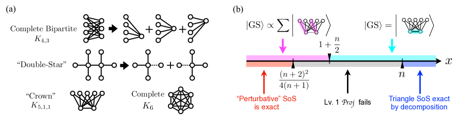
Figure 1: (a) Illustration of graphs where we provide exact $SoS$ in this section and how some of them could be decomposed. (b) The “phase diagram” of the crown graph with $n\geq 3$, where the true ground state is illustrated on the top, and regions where $SoS(\mathcal{Proj}_{1})$ gives exact solutions are shown on the bottom (colored in dark red and blue).

4.2.1 Crown Graphs

Graphs with one additional edge to $K_{n,2}$ ($n\geq 2$) connecting the two vertices of the B-sublattice (i.e. a complete tripartite graph $K_{n,1,1}$) also admits an exact $SoS_{1}(\mathcal{Proj})$ and thus $NPA_{1}(\mathcal{Proj})$ obtains the exact maximum eigenvalue as the upper bound. These graphs, which we call the “crown” graph (Fig. 1 (a)), have maximum eigenvalue $n+1$, the same value for the $K_{n,2}$ complete bipartite graphs. The additional edge does not change the maximum eigenvalue nor the maximum eigenvalue state itself.

We can modify the SoS in Eq. 85 so that the Hamiltonian now includes the one additional edge on the right hand side. If we label the two vertices in the B-sublattice to be $a$ and $b$, then the $SoS_{1}(\mathcal{Proj})$ reads

$$\frac{2}{n+1}\sum_{k=a,b}\Bigl{(}\frac{n+1}{2}\mathbb{I}-\sum_{i\in A}h_{ik}-\frac{2+n\pm n}{4}h_{ab}\Bigr{)}^{2}+\frac{2}{n+1}\sum_{i<j\in A}h_{ij}^{2}~{}=~{}(n+1)\mathbb{I}-H,$$ (86)

where there is a degree of freedom for the coefficient of $h_{ab}$, coming from two solutions of a quadratic equation.

The observation that the only difference between this SoS and Eq. 85 is the $h_{ab}$ term encourages us to ask if this form of SoS is general in some sense. Indeed, as it turns out, we can consider a crown graph with the term $h_{ab}$ being weighted with weight $x$, and the above form of the SoS is exact for the entirety of $x\leq(n+2)^{2}/4(n+1)$. The precise $SoS_{1}(\mathcal{Proj})$ becomes

$$(n+1)\mathbb{I}-\biggl{(}\sum_{k=a,b}\sum_{i\in A}h_{ik}+xh_{ab}\biggr{)}$$ (87)

$$= \frac{2}{n+1}\sum_{k=a,b}\Bigl{(}\frac{n+1}{2}\mathbb{I}-\sum_{i\in A}h_{ik}-\frac{2+n\pm\sqrt{(n+2)^{2}-4(n+1)x}}{4}h_{ab}\Bigr{)}^{2}+\frac{2}{n+1}\sum_{i<j\in A}h_{ij}^{2},$$

which only has a real solution when $x\leq(n+2)^{2}/4(n+1)$.

We can regard this SoS to be heuristically constructed in two steps. First, the case corresponding to $x=0$ was decomposable as in Eq. 84, yielding an SoS that retains the symmetry of the graph ($\mathbb{Z}_{2}$ between $a$ and $b$, and $\mathcal{S}_{n}$ for the A-sublattice sites). Next, when another edge is added also in a symmetry-preserving way, we can have an ansatz for the SoS that also still preserves the symmetry but now also includes the additional term. In this sense, the above SoS could be thought of as a “perturbative” SoS from the complete-bipartite case, since if we gradually increase $x$ from 0, the SoS also can be changed continuously, always being exact. Since $1<(n+2)^{2}/4(n+1)$, the uniformly weighted crown graph is also exactly solvable, and we can say that the $SoS_{1}(\mathcal{Proj})$ for the complete bipartite graph and the crown graph are adiabatically connected. Intuitively, when $x$ is small enough, the “physics” should not change a lot from the $x=0$ case, and in this case we can show that the “radius of convergence” extends to $x=(n+2)^{2}/4(n+1)$, including $x=1$.

The fact that the ansatz fails alone does not necessarily imply that no exact SoS exist, but it does suggest that even if such $SoS_{1}(\mathcal{Proj})$ exist, it will look very different from the SoS in the $x\leq(n+2)^{2}/4(n+1)$ region. As a matter of fact, we numerically observe that $NPA_{1}(\mathcal{Proj})$ starts to have nonzero error exactly from $x=(n+2)^{2}/4(n+1)$, implying that such a SoS proof indeed does not exist.

Conversely, when we increase $x$ large enough, $NPA_{1}(\mathcal{Proj})$ starts to obtain the exact ground state energy again starting from $x\geq n$. Intuitively, in the $x\rightarrow\infty$ limit, the ground state should trivially become a state where there is simply one singlet placed for $h_{ab}$, and it seems natural for an SDP algorithm to be able to obtain such a simple state exactly. This intuition could be made rigorous by noticing that when $x\geq n$, the Hamiltonian regains the decomposition property, but now into triangles:

$$H=\sum_{i\in A}\biggl{(}h_{ia}+h_{ib}+\frac{x}{n}h_{ab}\biggr{)},~{}~{}~{}\|H\|=\sum_{i\in A}\Bigl{\lVert}h_{ia}+h_{ib}+\frac{x}{n}h_{ab}\Bigr{\rVert}\text{ when }x\geq n.$$ (88)

Since a triangle with weight $(1,1,\alpha)$ has the exact $SoS_{1}(\mathcal{Proj})$ of

$$\begin{split}&\left(\alpha+\frac{1}{2}\right)\mathbb{I}-(h_{12}+h_{23}+\alpha h_{13})\\ =&\left(\alpha+\frac{1}{2}\right)\biggl{\{}\mathbb{I}-\sum_{1\leq i<j\leq 3}\frac{4\alpha+2\pm(-\frac{1}{2}+(-1)^{i+j})\sqrt{2\alpha(2\alpha-1)-2}}{3+6\alpha}h_{ij}\biggr{\}}^{2},\end{split}$$ (89)

for $\alpha\geq 1$, together with the decomposition, this can be turned into an $SoS_{1}(\mathcal{Proj})$ for the crown graph when $x\geq n$. Note that again, the SoS is not unique, and it has a degree of freedom in choosing $\pm$ to be fixed. When $\alpha<1$ the above form no longer gives a real coefficient. However, the true ground state of the triangle also changes, and still allows an exact $SoS_{1}(\mathcal{Proj})$:

$$\frac{3}{2}\mathbb{I}-(h_{12}+h_{23}+\alpha h_{13})=\frac{3}{2}\left(\mathbb{I}-\frac{2}{3}h_{12}-\frac{2}{3}h_{23}-\frac{2\pm\sqrt{6(1-\alpha)}}{3}h_{13}\right)^{2},$$ (90)

which again only gives valid coefficients for $\alpha\leq 1$. For our current objective of constructing a $SoS_{1}(\mathcal{Proj})$ for the crown graph, the existence of SoS for $\alpha<1\Leftrightarrow x<n$ does not help since the Hamiltonian no longer has the decomposition Eq. 88.

Again, like the case for the small $x$ region, although this decomposition is just one possible heuristic method for finding the exact SoS, it turns out that the $NPA_{1}(\mathcal{Proj})$ does start to fail exactly for $x<n$. Furthermore, it is possible to prove this failure for the region $(n+2)/3<x<n$ which rigorously establishes the right-side boundary at $x=n$ but leaves an unproved open space for the left-side boundary at $x=(n+2)^{2}/4(n+1)$. We provide this proof in Appendix C.1. The situation for the whole $x\in\mathbb{R}$ is illustrated in Fig. 1 (b). It is rather intriguing that the “phase transition” points for the SDP ($x=(n+2)^{2}/4(n+1)$ and $n$), and the phase transition for the true ground state ($x=1+n/2$) are well-separated. This means that there are broad regions of the $x$ parameter where the SDP algorithm fails despite having exactly the same ground state as other points where SDP succeeds, which interestingly seems to be caused by the lack of real solutions in a quadratic equation Eq. 89. In Section 5.2.1 and Section 5.2.2, we will see more nontrivial phase transitions in condensed matter physics models.

4.2.2 Double Star Graphs

While the crown graphs do not have the nice decomposition property that the complete bipartite graphs had, the double-star graphs have such a decomposition into two weighted star graphs. The double-star graphs are the ones with $n$ vertices connected to one vertex $a$, and the other set of $n$ vertices all connected to the other vertex $b$, and having an edge between $a$ and $b$ (thus $2n+2$ vertices in total).

In this case, the decomposition works as

$$H=\left(\frac{1}{2}h_{ab}+\sum_{i=1}^{n}h_{ai}\right)+\left(\frac{1}{2}h_{ab}+\sum_{j=n+1}^{2n}h_{bj}\right),~{}~{}~{}\|H\|=\biggl{\lVert}\frac{1}{2}h_{ab}+\sum_{i=1}^{n}h_{ai}\biggr{\rVert}+\biggl{\lVert}\frac{1}{2}h_{ab}+\sum_{j=n+1}^{2n}h_{bj}\biggr{\rVert},$$ (91)

and the SoS reduces to the case of a weighted graph (with only one edge having weight $1/2$). While the existence of exact $SoS_{1}(\mathcal{Proj})$ is provable for arbitrary weighted star graphs [Hwa+22a], for the particular case corresponding to the double star we can have relatively simple analytical forms:

$$\sum_{x=a,b}\biggl{\{}\biggl{(}\frac{E}{2}\mathbb{I}-\frac{2}{E}\sum_{i\in\partial x}h_{ix}-\frac{1}{E}h_{ab}\biggr{)}^{2}+\frac{1}{E}\sum_{i\neq j\in\partial x}h_{ij}^{2}~{}~{}~{}~{}~{}~{}$$ (92)

$$~{}~{}+\frac{\sqrt{n/(n+2)}}{2n+1}\sum_{i\in\partial x}\left(h_{iy}-\left(n+1-\sqrt{n(n+2)}\right)h_{ix}+\frac{1}{2E-2}h_{ab}\right)^{2}\biggr{\}}=E\mathbb{I}-H,$$

where $E$ denotes the maximum eigenvalue, i.e., $E=(n+2+\sqrt{n(n+2)})/2$, and $\sum_{i\in\partial x}$ indicates summation over all vertices $i$ that are the $n$ leaves adjacent to $x=a$ or $b$. $y$ denotes the vertex $a$ or $b$ other than the one chosen for $x$ in the summation.

While the above $SoS_{1}(\mathcal{Proj})$ shows that $NPA_{1}(\mathcal{Proj})$ obtains the ground state energy exactly for the double stars, the following $SoS_{2}(\mathcal{Proj})$ is simpler in form :

$$\sum_{x=a,b}\left\{\biggl{(}\alpha\mathbb{I}-\beta\sum_{i\in\partial x}h_{ix}-\gamma h_{ab}+\delta\sum_{i\in\partial x}h_{iy}\biggr{)}^{2}+\sum_{i\neq j\in\partial x}\left(\frac{\beta^{2}+\delta^{2}}{2}h_{ij}^{2}+2\beta\delta(h_{ix}h_{jy})^{2}\right)\right\}$$ (93)

$$= \frac{n+2+\sqrt{n(n+2)}}{2}\mathbb{I}-H,$$

where the specific coefficients are $\alpha=\sqrt{n+2+s}/2$, $\beta=(2\alpha+S)/(n+2)$, $\gamma=(2\alpha-(n+s)S/2)/(n+2)$, $\delta=((4\alpha^{2}-1)S-2\alpha)/(n+2)$, with $s=\sqrt{n(n+2)}$, and $S=\sqrt{(1+2/n)^{1/2}+s-n-2}$. Note that the $SoS_{1}(\mathcal{Proj})$ we provide here could again be viewed as an extension of the $SoS_{1}(\mathcal{Proj})$ for the complete bipartite case, just by adding another term to Eq. 86. Although this $SoS_{2}(\mathcal{Proj})$ Eq. (93) is weaker than $SoS_{1}(\mathcal{Proj})$ in terms of the SoS hierarchy, Eq. (93) straightforwardly shows that the “two-singlet density” $\langle h_{ix}h_{jy}\rangle$ is always 0, a piece of information that was not obvious from the $SoS_{1}(\mathcal{Proj})$ Eq. (92).

Interestingly, $NPA_{1}(\mathcal{Proj})$ starts to fail once the “double star” becomes imbalanced, i.e. having different number of leaves on the two sides. This implies that the decomposition of the double graph Eq. 91 only holds for very precise cases with balanced double graphs and does not exist in general.

4.3 Complete graphs: Contrast between even and odd

While the complete graphs $K_{n}$ do not admit similar decomposition as in Eq. 91, we can still obtain the exact $SoS_{1}(\mathcal{Proj})$ by exploiting the high symmetry of the graph – if the number of vertices $n$ is even:

$$\sum_{i=1}^{n}\left(\sqrt{\frac{n+2}{8}}\mathbb{I}-\sqrt{\frac{2}{n+2}}\sum_{j\neq i}h_{ij}\right)^{2}=\frac{n(n+2)}{8}\mathbb{I}-\sum_{1\leq i<j\leq n}h_{ij}.$$ (94)

Here again, the SoS is essentially a summation of the SoS for star graphs, but with slightly different coefficients, which makes them different from the simple decompositions we have been seeing.

The situation becomes quite different when the number of vertices is odd. The maximum eigenvalue is $(n+3)(n-1)/8$, but $NPA_{1}(\mathcal{Proj})$ gives $n(n+2)/8$ as the upper bound, which is $3/8$ bigger (observed numerically). We can see that for the odd case the $NPA_{1}(\mathcal{Proj})$ must do at least as good as $n(n+2)/8$ from the fact that the SoS we have above works perfectly fine even when $n$ is odd.

Ideally for odd $n$, the exact SoS should give

$$\frac{(n+3)(n-1)}{8}\mathbb{I}-\sum_{1\leq i<j\leq n}h_{ij}\succeq 0~{}~{}\Leftrightarrow~{}~{}\sum_{i<j}\left(X_{i}X_{j}+Y_{i}Y_{j}+Z_{i}Z_{j}\right)+\frac{3n-3}{2}\mathbb{I}\succeq 0.$$ (95)

Let $\ell^{*}$ be the smallest integer such that $NPA_{\ell^{*}}(\mathcal{Pauli}(H))=\mu_{max}(H)$. Since $NPA_{\ell}(\mathcal{Pauli})$ converges at $\ell=n$ we know $\ell^{*}\leq n$. By exploiting the $SU(2)$ symmetry of the LHS, we can see that obtaining a degree-$\ell$ SoS proof for

$$\sum_{i<j}Z_{i}Z_{j}+\frac{n-1}{2}\mathbb{I}\succeq 0~{}~{}\Leftrightarrow~{}~{}\left(\sum_{i=1}^{n}Z_{i}\right)^{2}\succeq\mathbb{I}$$ (96)

would be a sufficient condition for showing that $NPA_{\ell}(\mathcal{Pauli})=\mu_{max}\left(\sum_{i<j}h_{ij}\right)$. Since the Pauli operators $Z_{i}$ all commute, the problem essentially becomes classical and could be regarded as a MaxCut instance for the same odd complete graph. The problem then is equivalent to proving the following statement with SoS:

When you have odd numbers of $\pm 1$ values, their sum can never become 0.

This trivial statement about parity becomes surprisingly hard to prove with SoS and is known to require $\lceil n/2\rceil$-degree SoS [Gri01, Lau03, KM22], so $\ell^{*}\leq\lceil n/2\rceil$. While we believe that the same is most likely to be true for our case ($\ell^{*}=\Omega(n)$), we were only able to prove the impossibility with $SoS_{1}(\mathcal{Proj})$.

Theorem 4.5.

$NPA_{1}(\mathcal{Proj}(H))=n(n+2)/8$ for complete graphs with $n$ vertices, which gives the exact maximum eigenvalue when $n$ is even and is exactly $3/8$ larger than the exact maximum eigenvalue $(n+3)(n-1)/8$ when $n$ is odd.

Proof.

We show that the following constructed $M_{1}$ is a feasible solution for $NPA_{1}(\mathcal{Proj})$ that achieves the value $n(n+2)/8$. Together with the $SoS_{1}(\mathcal{Proj})$ in Eq. 94, this proves that the $NPA_{1}(\mathcal{Proj})$ gets the optimal value $n(n+2)/8$.

Now, consider the following moment matrix

$$M=\begin{pmatrix}1&a&a&\ldots&a&\ldots\\ a&a&a/4&\ldots&a/4&\ldots\\ a&a/4&a&\ldots&b&\ldots\\ \vdots&\vdots&\vdots&\ddots&\vdots&\\ a&a/4&b&\ldots&a&\ldots\\ \vdots&\vdots&\vdots&&\vdots&\ddots\end{pmatrix},$$ (97)

with

$$a=\frac{n+2}{4(n-1)},~{}~{}~{}b=\frac{n(n+2)}{16(n-1)(n-3)},$$ (98)

where the shown rows and columns are indexed by operators $\mathbb{I},h_{12},h_{13},\ldots,h_{24},\ldots$. In other words,

$$M(h_{ij},h_{kl})=\begin{cases}a,&(ij)=(kl),\\ a/4,&(ij)~{}\mathrm{and}~{}(kl)\mathrm{~{}have~{}exactly~{}one~{}overlap},\\ b,&(ij)~{}\mathrm{and}~{}(kl)\mathrm{~{}have~{}no~{}overlaps}.\end{cases}$$ (99)

It is easy to verify that this moment matrix has size $(1+{n\choose 2})\times(1+{n\choose 2})$, achieves energy $a\times{n\choose 2}=n(n+2)/8$, and satisfies the anti-commutation relation constraint: $((a+a-a)/2)/2=a/4$.

All we need to do now is to show $M\succeq 0$, and we do this by constructing Gram vectors of $M$ . Specifically, we construct $1+{n\choose 2}$ column vectors $\ket{\mathbb{I}}$ and $\{\ket{h}_{ij}\}$ for all $i,j\in[n]$ with $i<j$. Each column vector’s elements are also indexed with the operators $\mathbb{I}$ and $h_{ij}$ as well, which we will denote as the subscript below. We can then express the Gram vectors in the following way:

$$\ket{\mathbb{I}}_{\hat{O}} = \begin{cases}1,&\text{ if }\hat{O}=\mathbb{I}\\ 0,&\text{otherwise},\end{cases}$$ (100)

$$\ket{h_{ij}}_{\hat{O}} = \begin{cases}a,&\text{ if }\hat{O}=\mathbb{I}\\ \alpha,&\text{ if }\hat{O}=h_{ij}\\ \beta,&\text{ if }\hat{O}=h_{kl}\text{ (no overlap with $ij$) }\\ \gamma,&\text{ if }\hat{O}=h_{jk}\text{ (exactly one overlap with $ij$) },\end{cases}$$ (101)

with

$$\alpha=\frac{\sqrt{3(n-3)(n^{2}-4)}}{4\sqrt{{(n-1)^{3}}}},~{}~{}\beta=\frac{\sqrt{3(n+2)}}{2\sqrt{(n-1)^{3}(n-2)(n-3)}},~{}~{}\gamma=-\frac{\alpha}{(n-2)}.$$ (102)

It is straightforward to confirm that these vectors Eq. (100) and Eq. (101) are indeed Gram vectors for the moment matrix (Eq. 99) by a counting argument:

$$\braket{h_{ij}}{h_{ij}}= a^{2}+\alpha^{2}+{n-2\choose 2}\beta^{2}+(2n-4)\gamma^{2}=a=\braket{\mathbb{I}}{h_{ij}},$$ (103)

$$\braket{h_{ij}}{h_{kl}}= a^{2}+2\alpha\beta+{n-4\choose 2}\beta^{2}+(4n-16)\beta\gamma+4\gamma^{2}=b,$$ (104)

$$\braket{h_{ij}}{h_{jk}}= a^{2}+2\alpha\gamma+{n-3\choose 2}\beta^{2}+(2n-6)\beta\gamma+(n-2)\gamma^{2}=a/4,$$ (105)

thus concluding that $M$ is the optimal $M_{1}$ of $NPA_{1}(\mathcal{Proj})$ achieving the value $n(n+2)/8$. ∎

We can observe that the moment matrix that SDP creates is essentially “blind to the fact that $n$ is an integer” [GMZ22] and is the reason for obtaining the wrong value $n(n+2)/8$. This is the energy you would get when you naively plug in an odd number to the formula for even complete graphs. Motivated by this fact and realizing that most of the higher order terms in the higher level moment matrix would reduce to lower degree moments (just like $a/4$ in the example above), we conjecture that the only independent moment matrix elements in higher levels would be

$$\left\langle\overbrace{h_{ij}\cdot h_{st}\cdot\ldots}^{k\text{ independent op.s}}\right\rangle=\prod_{l=0}^{k-1}\left(\frac{n+2-2l}{4(n-2l-1)}\right),$$ (106)

which is the formula for an even complete graph, but simply formally replacing $n$ with an odd number, resembling the classical case [Gri01, Lau03, KM22]. All other matrix elements would be calculable from the projector algebra constraints.

5 Numerical results

While the SoS proofs in the previous section only cover a very small fraction of possible uniformly weighted graphs, the SDP algorithm actually solves surprisingly many graphs exactly, in the sense that the obtained upper bound value matches the exact maximum eigenvalue. This is true for both the $\mathcal{Pauli}$ and $\mathcal{Proj}$ SDP relaxations, and in this section we will go through the numerical results showing this. We further observe that the SDP algorithm can be used for calculating expectation values of operators that are of physical interest. This is demonstrated in section 5.2.3, where the $NPA_{1}(\mathcal{Proj})$ is applied to the Heisenberg Chain up to size $L=60$, and the critical correlation functions show the correct criticality up to error bars.

In the following of this section, the term “solve exactly” means that the upper bound value obtained by SDP theoretically matches exactly with the maximum eigenvalue.

5.1 Exhaustive numerical results on small graphs

Here, we show the results of $NPA_{2}(\mathcal{Pauli})$ applied to all possible uniform graphs up to $n=8$ vertices. The main observation is that $NPA_{2}(\mathcal{Pauli})$ is exact for many graphs with $n\leq 6$ vertices. While the percentage of such graphs seems to shrink as we go to larger system sizes, it suggests that there are many cases where an exact SoS exists that are not covered in the previous section.

5.1.1 Probing exact solvability numerically

Before presenting the main numerical results, here we address the subtle issue arising from numerical precision of the SDP algorithm. It is fundamentally impossible to determine whether the SDP algorithm obtains the correct energy value for a particular Hamiltonian solely from numerical results. This is because the SDP algorithm always requires a precision parameter which is usually referred to as “error-tolerance” $\epsilon$, and the algorithm only optimizes up to that $\epsilon$. Even if the algorithm seems to give very close values to the true energy we cannot a priori conclude if that is actually obtaining the exact solution, or if the error of the algorithm is merely small yet non-zero.

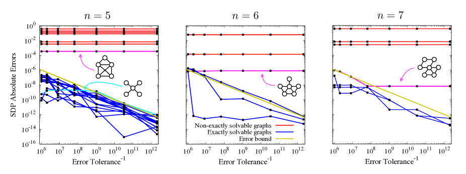
Figure 2: The absolute error of the energy with $NPA_{2}(\mathcal{Pauli})$ as a function of the tolerance parameter. For graphs with $n=5$ vertices, we show the curves for all possible 21 (connected) 5-vertex graphs, and for $n=6$ and 7, we only show a few randomly chosen graphs, since the number of the graphs becomes enormous (112 and 853 each). Blue and red lines correspond to cases exactly solvable and not respectively, and the magenta lines show the smallest errors that are nonzero.

To address this issue systematically, we analyzed the optimal value (upper bound of the maximum eigenvalue) obtained by the SDP algorithm as a function of the error tolerance. More precisely, as shown in Fig. 2, we plot the discrepancy of the SDP-obtained optimal value and the exact maximum eigenvalue $\Delta E:=|E_{\mathrm{SDP}}-E_{\mathrm{GS}}|$ as a function of $\epsilon^{-1}$. This plot, especially for $n=5$, shows a very clear dichotomy of $n=5$ connected graphs. While 7 graphs (red curves) have an almost constant $\Delta E>0$, the rest of the 14 graphs (blue curves) show a decay in $\Delta E$, roughly proportionally to $\epsilon$. This could be regarded as strong numerical evidence that the 14 graphs are exactly-solvable instances by the SDP algorithm while the 7 graphs are not. It is quite surprising that a simple five-vertex graph can naturally yield a very small error value around $0.00034$ (the graph shown in Fig. 2 with arrows in magenta).

However, we must note that this method is not entirely decisive. As depicted in the center and right panels of Fig. 2, the dichotomy becomes less clear as we go to larger sizes $n=6,7$, and is even worse for $n=8$ (not shown). This is because as we proceed to larger system size, an unweighted graph can potentially have extremely small error values $\Delta E$, such as $\sim 10^{-8}$ and even smaller. At some point, it practically becomes impossible, since smaller error tolerance $\epsilon$ requires longer iterations in the SDP optimization.

We can also see that the theoretical error bound of $\Delta E<\epsilon$ (drawn in yellow lines in the figure) for any exactly-solvable graph, is not necessarily satisfied always. For example, although we rigorously prove that the star graph is exactly solvable by the SDP algorithm (see §4.2), the error of the star graph in Fig. 2, $n=5$ (in cyan) is slightly above the error tolerance $\epsilon$. This arises from subtleties in how the error tolerances are handled inside the SDP package, and is difficult to control in general.

Despite these subtleties, the behavior of the absolute energy error $\Delta E$ as a function of the error tolerance $\epsilon$ serves as a good rule of thumb for distinguishing exactly-solvable graphs from instances with merely small errors. For instance, we can be fairly confident that the graphs with magenta arrows indeed do have extremely small but non-zero errors such as $\sim 10^{-6}$.

5.1.2 Exactly solvable small graphs and their statistics

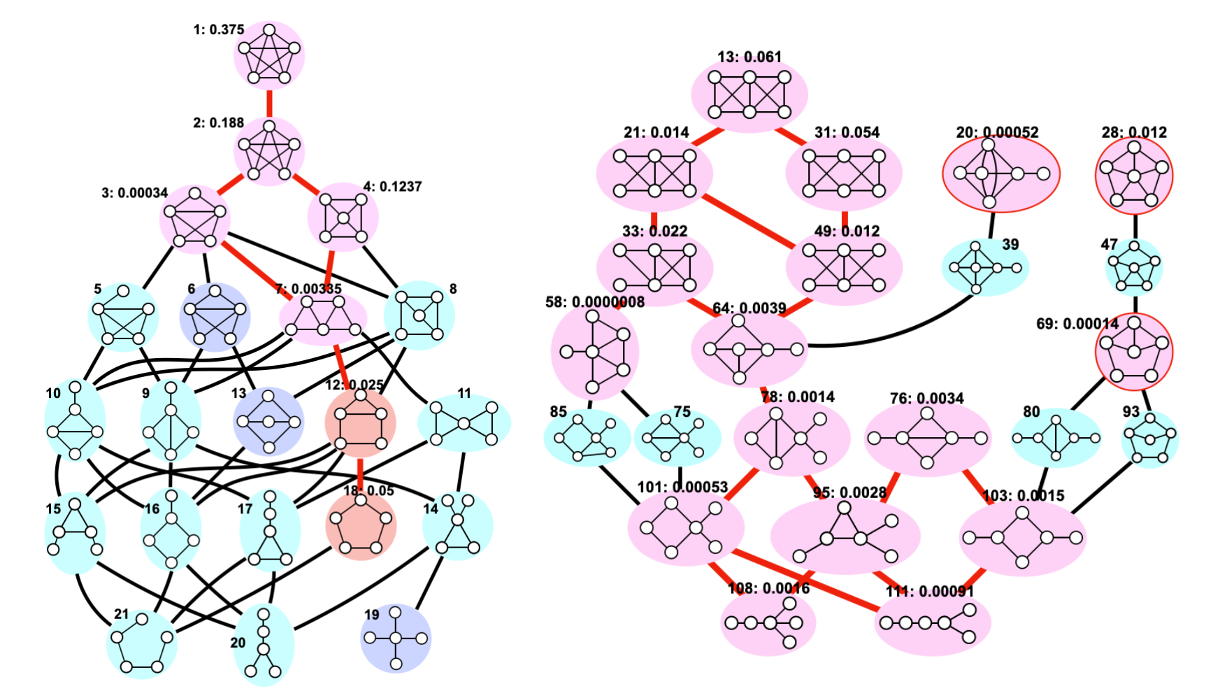
Figure 3: All graphs with $n=5,6$ which the level-2 Pauli basis SDP algorithm fails to obtain the true ground state energy, colored in red/magenta. The labeling of the graphs follows [CP84], and the values following the labels represent the error value $\Delta E$ from Lv. 2 Pauli SDP. For the $n=5$ diagram, we further distinguish graphs where we know an explicit construction of SoS (dark blue) and graphs where Lv. 2 Pauli SDP still fails even when adding a constraint on the total spin $S^{2}\geq 3/4$ (red).

Once we can confidently determine whether or not the SDP algorithm obtains the true ground state energy, we can start to ask questions such as “When and how often does the SDP algorithm give us the exact solution?”. To address this question, we present an exhaustive study for all connected graphs with $n=5,6,7$ and $8$ vertices.

Figure 3 shows all of the 7 (out of 21) $n=5$ connected graphs and the 17 (out of 112) $n=6$ connected graphs that the $NPA_{2}(\mathcal{Pauli})$ SDP algorithm fails to obtain the exact ground state energy (colored in red/magenta). The numbers are labeling of the graphs according to a convention introduced in [CP84]. It is rather surprising that the algorithm obtains the exact ground state energy for the vast majority of the graphs (colored in blue/cyan) up to this system size, noting that for most of the graphs the SoS is unknown and most likely very complicated (graphs in cyan).

The figure also shows the topological relations of the graphs, by connecting them with a thick bond whenever two graphs only differ by one edge. In this way, we can see that for $n=5$ the red/magenta graphs (SDP fail) form one cluster. In other words, any two $n=5$ connected graphs that Lv. 2 Pauli SDP fails, can be transformed into one from the other by adding and subtracting one edge at a time, always maintaining the SDP algorithm to be failing. This is not the case for $n=6$, where the magenta graphs seem to form one big cluster and also three disconnected “islands” (namely, graphs 20, 28, and 69). However, as we will see in the following, the “single-clusteredness” of the hard graphs recovers once we focus on the errors from the $NPA_{1}(\mathcal{Proj})$.

The “failing cluster” includes the complete graph for $n=5$ but not for $n=6$. This is exactly as expected as we explained in Section 4.3. This raises the question whether we can actually further constrain the SDP algorithm, not with a higher level, but simply by adding a constraint corresponding to the minimum total spin of the ground state. More specifically, the constraint would be

$$\sum_{1\leq i<j\leq n}M(\mathbb{I},h_{ij})\leq\frac{(n+3)(n-1)}{8},$$ (107)

from Eq. 95 for odd $n$. When we add this constraint, $NPA_{1}(\mathcal{Proj})$ not only was able to solve the complete graph $K_{5}$ exactly, but other graphs in the vicinity. This information is indicated in Fig. 3, by showing graph 12 and 18 in red, being the only two graphs that $NPA_{1}(\mathcal{Proj})$ with this additional constraint still failed. Note that we cannot do the same thing when we have even number of qubits, because $NPA_{1}(\mathcal{Proj})$ already succeeds for the complete graphs, i.e., already know about this constraint on total spin.

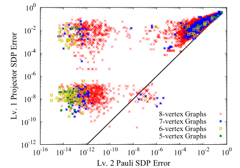
Figure 4: The energy errors from the SDP algorithm in two different bases for all graphs up to $n=8$ (left) and list of all $n=5$ and 6 graphs that $NPA_{2}(\mathcal{Pauli})$ is exact but $NPA_{1}(\mathcal{Proj})$ is not (right). The shaded graphs are the ones which $NPA_{2}^{\mathbb{R}}(\mathcal{Pauli})$ fails as well (it succeeds for all other graphs listed here). The labeling of the graphs follows [CP84].

We also compare the performance of the different SDP algorithms ($NPA_{2}(\mathcal{Pauli})$, $NPA_{2}^{\mathbb{R}}(\mathcal{Pauli})$, and $NPA_{1}(\mathcal{Proj})$) for all of these graphs up to $n=8$ in Fig. 4. The scatter plot shows the energy errors for $NPA_{2}(\mathcal{Pauli})$ and $NPA_{1}(\mathcal{Proj})$. The fact that the scattered points roughly forms four different clusters could be understood in the following way.

Firstly, the cluster on the top right corresponds to graphs that the SDP algorithms with either bases fail to obtain the exact ground state. If we believe in typical hardness of the random QMaxCut instances, the ratio of graphs in this cluster in the scatter plot should reach 1 in the large problem size limit. The fact that all of the points in this cluster are on the left of the black line indicating $x=y$ reflects the fact that the $NPA_{2}(\mathcal{Pauli})$ SDP can never perform worse than the $NPA_{1}(\mathcal{Proj})$ SDP. This could be easily seen from the fact that you can always convert an SoS proof using degree-1 polynomials of projectors into SoS that uses degree-2 Pauli polynomials, but not necessarily the other way around.

Whether the aforementioned inequality $NPA_{2}(\mathcal{Pauli}(H))\geq NPA_{1}(\mathcal{Proj}(H))$ is actually an equality or not for QMaxCut instances is not obvious until we actually see examples. The second cluster on the top left of Fig. 4 reflects exactly that there are indeed graphs where $NPA_{2}(\mathcal{Pauli})$ SDP is exact but $NPA_{1}(\mathcal{Proj})$ SDP fails, i.e., that the inequality is strict in general. We list up all the $n=5$ and 6 graphs that fall under this second cluster on the right side of Fig. 4. Furthermore, we also checked how $NPA_{2}^{\mathbb{R}}(\mathcal{Pauli})$ SDP performs on these graphs to find that the inequality $NPA_{1}(\mathcal{Proj}(H))>NPA_{2}^{\mathbb{R}}(\mathcal{Pauli}(H))>NPA_{1}(\mathcal{Pauli}(H))$ is also strict in general. Specifically, we find that $NPA_{2}^{\mathbb{R}}(\mathcal{Pauli})$ fails for all of the graphs shaded in Fig. 4, while it succeeds for all of the other graphs with $n=5$ and 6. This means that the exact Pauli SoS for unshaded graphs are “breaking the SU(2) symmetry” in the individual squares possibly by having one-body Pauli terms in them. Those effects must cancel out as a whole when all the SoS terms are added since the final Hamiltonian has SU(2) symmetry and has no one-body terms. For the shaded graphs, this “symmetry breaking” trick is not enough to obtain the exact SoS, and complex SoS are required to do so. As a concrete example, the graph labeled 8 in Fig. 4 has errors $1.4\cdot{}10^{-2}$, $5.7\cdot{}10^{-4}$ and $8.06\cdot{}10^{-12}$ for $NPA_{1}(\mathcal{Proj}(H))$, $NPA_{1}^{\mathbb{R}}(\mathcal{Pauli}(H))$ and $NPA_{1}(\mathcal{Pauli}(H))$ respectively, which we interpret as the complex Pauli hierarchy being exact on this instance, but the real Pauli and complex projector hierarchy have nonzero errors.

The third cluster on the bottom left corresponds to graphs where the SDP algorithm succeeds with either of the bases. The ratio of the graphs in this third category seems to decrease as we get to larger sizes of graphs, which we will discuss further later. Noticing that the separation between $NPA_{2}(\mathcal{Pauli})$, $NPA_{2}^{\mathbb{R}}(\mathcal{Pauli})$, and $NPA_{1}(\mathcal{Proj})$ are strict in general from the previous paragraph, it seems more natural to regard this cluster as instances where $NPA_{1}(\mathcal{Proj}(H))=0$ forces the other two SDPs to have 0 error as well. From this perspective, it is more intriguing when $NPA_{1}(\mathcal{Proj}(H))=NPA_{2}(\mathcal{Pauli}(H))>0$, i.e., exactly on top of the $x=y$ line in Fig. 4, but in the top right cluster. Up to $n=8$ connected graphs we have computed, the only cases when that happens are all graphs related to complete graphs (simplest cases discussed in Section 4.3).

There is a rather small fourth cluster on the right bottom, that extends beyond to the right side of the $x=y$ line. Since $NPA_{2}(\mathcal{Pauli})$ must always perform no worse than $NPA_{1}(\mathcal{Proj})$, this suggests a numerical error of some sort. We have observed that the SDP packages for these graphs do not converge as quickly as other graphs, and tends to give results that have larger duality gaps than specified. This practically does not become a problem since the errors are very small (around $10^{-6}$), and all graphs which we explicitly exemplify as “NPA failing” in this work are not from this group . Notably, instances falling on the right side of the $x=y$ line only occur at very small errors (bottom right), while none are observed in the top right cluster. This is encouraging, since we can be confident that these practically pathological cases only arise when we demand high numerical precision. This allows us to consider all of the graphs in the fourth cluster (bottom right) to be theoretically easy for both bases of SDP, i.e., actually belonging to the third cluster (bottom left).

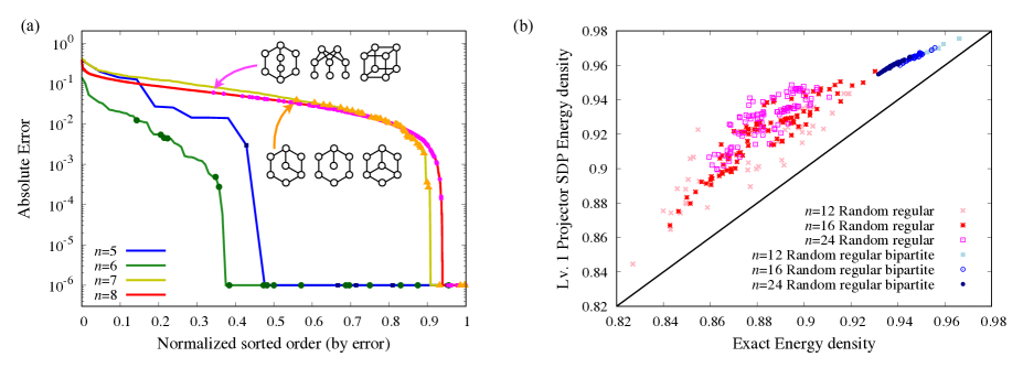
Figure 5: (a) Absolute error values $E_{\mathrm{SDP}}-E_{\mathrm{GS}}$ for all connected graphs with $n=5,6,7$ and $8$ vertices, shown in descending order for each $n$. All error values smaller than $10^{-6}$ can be regarded as 0, and is displayed as $10^{-6}$ for visual simplicity. We show points corresponding to bipartite graphs with points on top of the curves, showing the general tendency of bipartite graphs having relatively smaller errors. We also illustrate the top three bipartite $n=8,7$ graphs with largest errors. (b) The scatter plot of random regular graphs and random regular bipartite graphs with degree 3 and size $n=12,16$ and 24 qubits, 100 samples each.

In order to see the statistics of the errors more closely, in Fig. 5 (a), we show the values of the error for the $NPA_{1}(\mathcal{Proj})$ SDP in descending order for each size of graphs $n=5,6,7$ and $8$. The $x$-axis is rescaled so that the data of 21, 112, 853, and 11,117 graphs all fit into $[0,1]$. Thus, the figure is the inverse of the cumulative distribution function of errors.

For example, all four curves display an acute decline at some point corresponding to the separation between graphs that have nonzero errors and (essentially) zero error. The graph shows that the ratio of such non-exactly solvable graphs are roughly $46\%,37\%,91\%$ and $94\%$ among all connected $n=5,6,7$ and $8$-vertex graphs respectively. This means that the ratio of exactly solvable graphs tend to decrease as the number of vertices increases, possibly converging to 0 in the $n\rightarrow\infty$ limit. Yet still, the actual number of connected graphs that are exactly solvable seems to grow with $n$ at least for this size regime: 11, 67, 77, and 670, for $n=5,6,7$ and 8.

Another piece of information in the graph, represented as the points in the figure, is how the bipartite graphs are distributed among this descending-error ordering. The QMaxCut problem on bipartite graphs is oftentimes described as having “no geometric frustration” in condensed matter physics, since the singlet projector $h_{ij}$ could be seen as a constraint that favors the two qubits to be pointing in the opposite direction. From this point of view, we would consider an odd-length loop as geometrically frustrated because the interaction would not be (even relatively) satisfied with a simple approach of having the qubits point the opposite directions alternately. This difference has practical applications, such as bipartite cases allowing the quantum Monte Carlo method to efficiently obtain the ground state classically. Therefore, it is not so surprising that the bipartite graphs in Fig. 5 (a) are distributed relatively on the right side of each curves, implying (exponentially) smaller errors. In some sense, the surprise is in the other direction, that SDP fails to obtain the exact ground states of such “easily classically simulable” instances most of the time. It is unclear if the tendency of bipartite graphs having relatively small errors will remain for larger $n$, since it is already apparent that the position of the largest-error bipartite graph shifts to the left in Fig. 5 (a) from $n=7$ to $n=8$.

In order to test the difference between bipartite graphs and non-bipartite graphs in a more systematic way, we also ran the SDP algorithm for random regular graphs with degree-3. When such graphs are generated uniformly randomly, for sufficiently large $n$, the graph is almost certainly non-bipartite. We generate 100 of such samples, and compare the performance of $NPA_{1}(\mathcal{Proj})$ against exact diagonalization for $n=12,16$ and 24. It is also possible to generate uniformly random graphs that are bipartite and regular, and both results are displayed in Fig. 5 (b). It is immediately apparent that the non-bipartite random regular graphs have a broader distribution in the two-dimensional scatter plot, compared to the bipartite cases. The cluster is also located farther away from the $x=y$ line in black, showing a larger relative error compared to bipartite random graphs. The bipartite random graph data also seem to form a “line” in the scatter plot, indicating that the optimal SDP objective can give a fairly narrow estimate of the true energy value by a properly fitted linear function. In contrast, the non-bipartite random graph data extends in a two-dimensional manner forming a oval-like shape, resulting in broader estimates of the true energy given the SDP energy.

5.1.3 Transition points in the solvability of small graphs

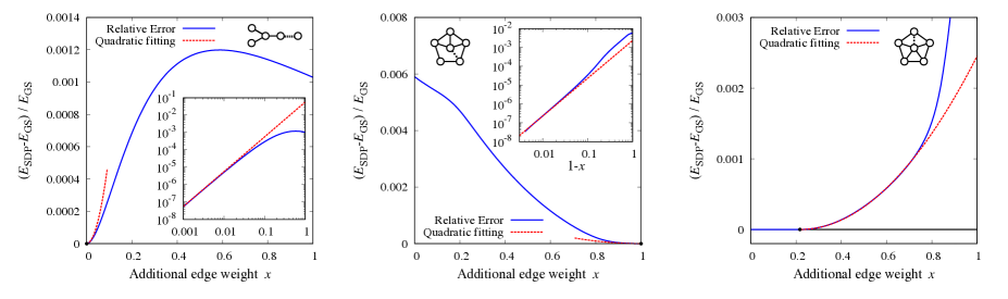
Figure 6: Three different cases of adding an additional edge to a graph with weight $x$, resulting in the change of solvability with $NPA_{1}(\mathcal{Proj})$. The insets show the log-log plot to clarify the matching of the quadratic fitting near the transition.

The clusteredness of hard and easy graphs shown in Fig. 3 leads to the question of what happens at the boundary between them. If there is a pair of graphs which one is exactly solvable while the other is not, with only one edge difference as graphs, then we can add that one different edge with weight $x\in[0,1]$. This procedure continuously connects the graphs and demonstrates where exactly SDP starts to fail.

In Fig. 4, we show three different cases of such a procedure. On each panel, we show the graph we use for demonstration, with the dotted edge being the weighted one. The left most panel shows the case for interpolating between the $n=4$ star graph and the Y-shaped $n=5$ graph (graph # 20 in Fig. 4 (a)), which is the easiest case of such. In this case, we can see that the moment we add $\epsilon>0$ amount of the new edge, SDP starts to fail. This could be argued that the solvability of the star graph in this situation is rather fragile, and immediately fails when perturbed away.

The same thing could be argued for the case shown in the middle panel connecting graph #69 and #47 of Fig. 3 right. Again in this case, the moment the graph diverges away from the exactly solvable #47, the SDP algorithm starts to fail. However, there exist cases where the “transition” happens not at the edges but at a nontrivial value, as shown in the right panel. The error becomes as small as the duality gap set for the SDP solver for $x<0.22$. In this case, we can say that the solvability of graph #47 is somewhat robust, and survives the perturbation in the direction considered here (towards graph #28).

Curiously, for all cases we have checked for interpolations between solvable and unsolvable graphs with $NPA_{1}(\mathcal{Proj})$, we always observe a quadratic initial increase of the error, as shown with the red dotted lines in Fig. 6. The quadratic fit is extremely good at the vicinity of the “transition points” where the error starts to become nonzero, as shown in the insets of the figures. This resembles universal critical behavior seen in physics, where phase transition points vary largely depending on the details of the statistical physics model, but an indicator of the phase transition (called the order parameter) behaves as $\propto|T-T_{c}|^{\beta}$ with a universal exponent denoted by $\beta$. Although our observed exponent $\beta=2$ is clearly present numerically, we were unable to provide a general explanation, and leave it for future studies.

5.2 Numerical results for some condensed matter physics models

Here, we demonstrate the power of the SDP algorithm when applied to a number of condensed matter physics models. The message is two-fold: first, the SDP algorithm could be used to probe exact-solvability of models in some settings, giving rise to the possibility of numerical exploration for exactly-(analytically) solvable systems. Second, the method could be seen as the first-order approximation of the ground state, it actually gives very accurate numbers in practice, with errors only up to $\sim 4\%,7\%,2\%$ for the models we study.

Both the Majumdar-Ghosh model and the Shastry-Sutherland model are known to be “frustration-free” in the quantum spin system literature [Bea+10, Sat+16, WKS21, AAG22]. This means that the Hamiltonian could be rewritten as sum of terms that could all be satisfied simultaneously in the ground state. The standard way to show this is to rewrite the physical Hamiltonian (thus with the opposite sign from our QMaxCut convention as in Eq. (21)) as a sum of projectors with additive and multiplicative constants. If there exists a state that the all the projectors evaluate to 0, that must be the ground state (note that the physics convention here is a minimization of the eigenvalue).

Because all projectors are square of themselves, we can immediately obtain an SoS of some degree by flipping the entire sign, and redefining the Hamiltonian with the QMaxCut convention. In most cases in physics, the definition of “frustration-free” requires the rewritten terms of the Hamiltonian to be spatially local. Thus, the SoS hierarchy could be seen as a generalization of the frustration-free notion, where we do not necessarily require spatial locality, but restrict the degree of the terms as polynomials. The fact that the degree-restriction could be arbitrarily relaxed by the level of the hierarchy, and that SDP algorithms can solve the optimization problem efficiently for $\mathcal{O}(1)$ level, provides us a systematic approach to explore frustration-free Hamiltonians in a computational way.

5.2.1 The Majumdar-Ghosh model

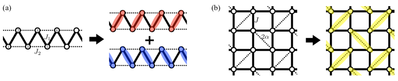
Figure 7: The graph structures of the (a) $J_{1}$-$J_{2}$ model and (b) the Shastry-Sutherland model. The exactly solvable ground states for both models are also illustrated where the colored ovals represent singlet pairs.

The Majumdar-Ghosh (MG) model [MG69] was one of the earliest proposed quantum spin models where the ground state could be obtained exactly. The Hamiltonian being considered is

$$H=\sum_{i=1}^{L}\Bigl{(}J_{1}h_{i,i+1}+J_{2}h_{i,i+2}\Bigr{)},$$ (108)

where we use the QMaxCut convention (i.e. the “ground state” we are searching for now is the maximum eigen state of this operator). The lattice structure is shown in Fig. 7(a). The Hamiltonian above would typically be referred to as the $J_{1}$-$J_{2}$ Heisenberg chain in the context of condensed matter physics, and the MG model corresponds to the case where $J_{2}/J_{1}=1/2$, also known as the MG point. At the MG point, the ground state is two-fold degenerate with two different singlet-product states where closest neighbors are forming singlets periodically, as depicted in Fig. 7(a):

$$|\mathrm{GS}\rangle=\prod_{i\in\mathrm{even}}^{\otimes}|s_{i,i+1}\rangle+\prod_{i\in\mathrm{odd}}^{\otimes}|s_{i,i+1}\rangle,$$ (109)

where by $|s_{i,j}\rangle$ we denote a singlet state between the spins on sites $i$ and $j$.

The exact ground state could be understood from the fact that the Hamiltonian at the MG point decomposes in the same sense of Eq. (84). Specifically,

$$H=\frac{J_{1}}{2}\sum_{i=1}^{L}\Bigl{(}h_{i,i+1}+h_{i+1,i+2}+h_{i,i+2}\Bigr{)},~{}~{}~{}~{}\lVert H\rVert=\frac{J_{1}}{2}\sum_{i=1}^{L}\Big{\lVert}h_{i,i+1}+h_{i+1,i+2}+h_{i,i+2}\Big{\rVert}$$ (110)

holds. Since the individual terms after this decomposition reduces to a triangle with equal weights, we can reuse the exact $SoS_{1}(\mathcal{Proj})$ from Eq. (90), obtaining

$$\frac{3L}{4}\mathbb{I}-H=\sum_{k=1}^{L}\frac{3J_{1}}{2}\biggl{\{}\mathbb{I}-\frac{2}{3}\bigl{(}h_{k-1,k}+h_{k,k+1}+h_{k-1,k+1}\bigr{)}\biggr{\}}^{2}$$ (111)

for the periodic boundary condition ($L+i\equiv i$). This corresponds to the standard projector expression for frustration-free models as we mentioned earlier, and implies that $NPA_{1}(\mathcal{Proj})$ is able to obtain the exact ground state energy at the MG point.

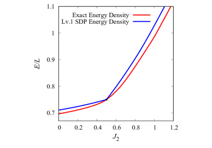
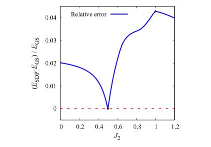
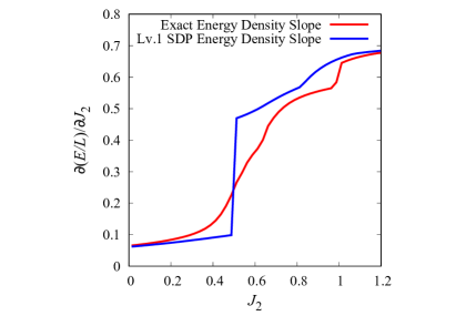
Figure 8: Performance of the SDP algorithm for the the size $L=16$ $J_{1}$-$J_{2}$ model with periodic boundary condition and $J_{1}=1$ fixed. Comparison is made between the exact ground state energy $E_{\mathrm{GS}}$ and the values obtained by the Lv.1 singlet projector SDP algorithm $E_{\mathrm{SDP}}$. The energy densities (left) are very close, and we can see that the relative error (center) becomes exactly 0 at the MG point. When we take the derivative of the energy densities (right), the SDP algorithm actually detects the MG point at $J_{2}/J_{1}=1/2$ in the model way more sharply compared to the exact solution, at this system size.

This is demonstrated in Fig. 8, where we compare the exact energy $E_{\mathrm{GS}}$ and the SDP energy $E_{\mathrm{SDP}}$ for the $L=16$ case with periodic boundary condition. The fact that the SDP algorithm obtains the exact ground state energy is reflected as the two energy density values coinciding at the MG point in the left panel, and correspondingly in the center panel the relative error becomes 0. Interestingly, the SDP algorithm seems to be “more sensitive” to the MG point in this $J_{1}$-$J_{2}$ model compared to the actual ground state energy, when we try to detect it by looking into the derivatives of the energy (right panel).

The fact that in Fig. 8 we see the SDP algorithm only obtaining the energy exactly at the MG point establishes that there are no other exactly-solvable points in the $J_{1}$-$J_{2}$ model, even if we allow non-local terms as long as they are limited to degree-2 in polynomials of singlet projectors.

5.2.2 The Shastry-Sutherland model

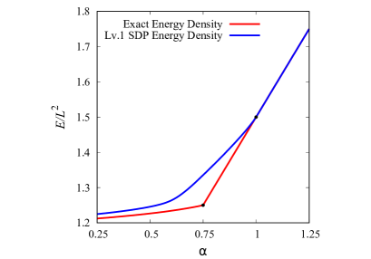
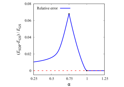
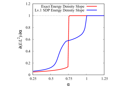
Figure 9: Performance of the SDP algorithm for system size $n=L^{2}=16$ Shastry-Sutherland model with periodic boundary condition. Comparison is made between the exact ground state energy $E_{\mathrm{GS}}$ and the values obtained by the Lv.1 singlet projector SDP algorithm $E_{\mathrm{SDP}}$. The energy densities (left) are very close, and we can see that the relative error (center) becomes exactly 0 for $\alpha\geq 1$. When we take the derivative of the energy densities (right), the SDP algorithm seems to be detecting the two phase transitions in the model more sharply compared to the exact solution, at this system size.

The Shastry-Sutherland (SS) model [SS81] is a two-dimensional Heisenberg model that also admits an exact ground state representation for a certain parameter region. The Hamiltonian in the QMaxCut convention would read

$$H=J\sum_{\langle ij\rangle}h_{ij}+2\alpha\sum_{\langle\langle ij\rangle\rangle}h_{ij}$$ (112)

where $\langle ij\rangle$ represents bonds of the $L\times L$ square lattice (with periodic boundary condition) and $\langle\langle ij\rangle\rangle$ represents diagonal bonds of the Shastry-Sutherland lattice as illustrated in Fig. 7(b). For simplicity, we fix $J=1$.

This model has an obvious unique ground state when $\alpha$ is large enough, since the diagonal bonds with weight $2\alpha$ gives a perfect matching of the sites. In that parameter region, the unique ground state could be written as

$$|\mathrm{GS}\rangle=\prod_{\langle\langle ij\rangle\rangle}^{\otimes}|s_{i,j}\rangle,$$ (113)

again illustrated in Fig. 7(b).

For the SS model with $\alpha>1$, we are again able to decompose the Hamiltonian into triangles with weights 1, 1, and $\alpha$, as previously discussed in section 4.2.1. It is easy to check that the Shastry Sutherland lattice (Fig. 7 (b)) can be decomposed into such triangles geometrically, with all triangles having two edges from the square lattice and one from the diagonal edges. Now, we can reuse Eq. (89) to obtain

$$\left(\alpha+\frac{J}{2}\right)N\mathbb{I}-H$$ (114)

$$= \sum_{\triangle}\left(\alpha+\frac{J}{2}\right)\biggl{\{}\mathbb{I}-\sum_{\mathrm{edges}\in\triangle}\frac{4\alpha+2J\pm(-2)^{j}\sqrt{2\alpha(2\alpha-J)-2J^{2}}}{3J+6\alpha}h_{\mathrm{edge}}\biggr{\}}^{2},$$

which gives the exact value only when $\alpha\geq J$. The summation $\sum_{\triangle}$ is taking the summation for all right triangles in the SS lattice as in the decomposition, and the summation inside of the square is for the three different edges for each such triangle. The $(-2)^{j}$ factor only appears for the edges with weight $J$ belonging to the square lattice where we set $j=1$, and not for the diagonal edges with weight $\alpha$ which we set $j=0$. Just as in Eq. (89), the SoS has a degree of freedom in choosing $\pm$ for the square root term.

In Fig. 9, we demonstrate the performance of the $NPA_{1}(\mathcal{Proj})$ SDP algorithm applied to the SS model with system size $n=L^{2}=16$ and $J=1$ fixed. We can see that the algorithm obtains the exact ground state energy for the entirety of the $\alpha\geq 1$ region, which exactly coincides where Eq. (114) gives a proper SoS (otherwise it has no real coefficients), and also the decomposition exists. The true ground state actually becomes the dimer singlet state Eq. 113 from $\alpha\geq 3/4$ for this system size, although the SDP algorithm fails to obtain that. This means that while $\alpha\geq 1$ was the condition used to show frustration-freeness in [SS81], relaxing the notion to allow non-local terms (but still only having degree-1 terms in the SoS) does not enlarge the region of exact-solvability. It would be interesting to see how the exactly solvable region changes as a function of the level of the NPA hierarchy.

Furthermore, by looking at the first derivative of the SDP energy as a function of $\alpha$, we can clearly see that there are two points where $\partial E/\partial\alpha$ has a singularity (Fig. 9 right), namely $\alpha\simeq 0.73$ and $\alpha=1$. The existence and the nature of different phases in the SS model is actively discussed in the condensed-matter physics context, where there is expected to be at least two phase transition points, i.e., singular points [KK00, Lee+19, YSW22]. The fact that the SDP energy derivative exhibit two singular points from relatively small system sizes suggest the possibility of this approach be used to detect phase transitions in similar models, without relying on comparison with exactly obtained ground states. The SDP algorithm also allows us to calculate observables other than energy such as the squared Néel order parameter from the moments, with a guarantee that they converge to the true value when the NPA hierarchy converges to the true ground state energy value. This lets us to interpret such physical observables obtained this way to be regarded as a first-order approximation. In the next section we see that even such approximated quantities can show essential characteristics in physical systems.

Another thing to note is that both Hamiltonians for the SS model and the MG model allowed decomposition of the Hamiltonian as in Eq. 84 and Eq. 91. In the cases of SS and MG models, the sub-Hamiltonians were the triangles with $\alpha,J,J$ bonds and $J_{1}/2,J_{1}/2,J_{2}=J_{1}/2$ bonds respectively. However, it should be noted that the existence of such decomposition is not a necessary condition for obtaining exact SoSs. For example, for the crown graph which we present an exact SoS in section 4.2.1, it appears that there are no such decomposition, while still having an exact SoS. The same could be said for complete graphs with even number of vertices. This fact gives us hope on discovering new exactly-solvable Hamiltonians, since oftentimes the search for frustration-free Hamiltonians relies on the existence of such decomposition [Gho23, Kum02].

5.2.3 The Heisenberg chain

The nearest neighbor antiferromagnetic Heisenberg chain is one of the simplest yet nontrivial quantum spin system that also happens to be a QMaxCut instance. The Hamiltonian we consider here is simply the chain

$$H=\sum_{i=1}^{L}h_{i,i+1},$$ (115)

with a periodic boundary condition $L+k\equiv k$. This corresponds to setting $J_{2}=0$ for the $J_{1}$-$J_{2}$ model in section 5.2.1. Although the Heisenberg chain has an exact solution thanks to the Bethe ansatz [Bet31], the exact solvability of the model is quite different from the previous two models: it does not involve frustration-freeness, and our SDP algorithm is therefore not expected to solve it exactly.

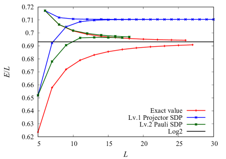
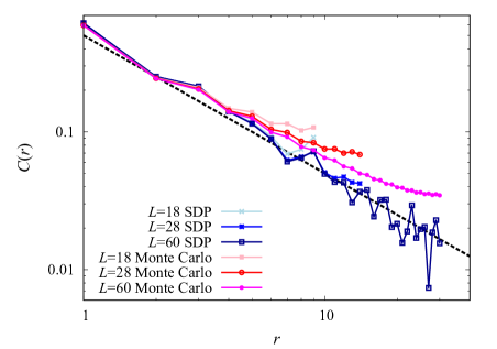
Figure 10: Performance of the SDP algorithm on the Heisenberg chain with periodic boundary conditions(cycle graphs). The left panel shows the exact and SDP obtained energy densities for system sizes $L=5$-$30$. In the thermodyanmic limit $L\rightarrow\infty$, the true energy density converges to $\log 2$. The right panel shows the correlation function $C(r)$ as a function of distance, both obtained by Lv. 1 projector SDP and quantum Monte Carlo (essentially exact). The dotted line shows the theoretically known asymptotic decay exponent $C(r)\propto r^{-1}$.

In the left panel of Fig. 10, we show our numerical results on how the SDP algorithm performs on the Heisenberg chain, by comparing the $NPA_{1}(\mathcal{Proj})$, $NPA_{2}(\mathcal{Pauli})$, and the exact value for various system sizes. We plot the energy density $E/L$ here, so the fact that all three cases converge to different values indicate that the absolute error of the total energy increases linearly with the system size $L$ for large enough $L$. Still, the qualitative behavior of approaching the limiting value from above and below for even and odd $L$ is reproduced in both of the SDP methods.

In the right panel, we show the correlation function

$$C(r):=\langle\mathrm{GS}|(-1)^{r}Z_{i}Z_{i+r}|\mathrm{GS}\rangle=(-1)^{r}\frac{1-4~{}M(\mathbb{I},h_{i,i+r})}{3},$$ (116)

obtained by $NPA_{1}(\mathcal{Proj})$ and Monte Carlo (virtually exact value) for system sizes $L=18,28,$ and $60$. Note that the translation symmetry of the cycle ensures the well-definedness of $C(r)$ regarding the choice of $i$ in the definition. The second equality in Eq. 116 is valid only in the case where the SDP algorithm obtains the exact ground state. However, we can still measure the RHS quantity even in cases where the algorithm fails and consider the obtained result as an approximation. Remarkably, when utilizing the SDP-obtained correlation function in this manner, it aligns very well with the true correlation function for small values of $r$ as shown in the figure. This can be attributed to the fact that the energy density exhibits a relative error of only $\sim 2\%$.

One characteristic feature of the Heisenberg chain is that the ground state displays a power-law decaying correlation with critical exponent $\eta=1$, i.e., $C(r)\propto r^{-1}$, which is closely linked to the long-range entanglement it has. The fact that the SDP-obtained correlation function displays the same type of power-law decay with essentially the correct exponent (albeit the jagged feature) is quite interesting especially when it is compared to the exact correlation function of finite systems, since it appears to have even smaller finite-size corrections. This raises the intriguing possibility that SDP-derived quantities capture the underlying “physics” of the ground state, even when there is no physical quantum state corresponding to the optimal moment matrix.

Finally, an alert reader may notice from the figure that both $NPA_{1}(\mathcal{Proj})$ and $NPA_{2}(\mathcal{Pauli})$ are exact for the $L=6$ hexagon case. Although we were unable to obtain an analytic $SoS_{1}(\mathcal{Proj})$, we were able to study the structure of the ground state from the SDP perspective, which we provide in Appendix D.

6 Acknowledgements

We thank Claudio Procesi for bringing to our attention several important references. J.T. thanks Hosho Katsura, Cristopher Moore, Sho Sugiura, and Seiji Takahashi for valuable discussions. C.Z. thanks Michał Adamaszek from MOSEK for helpful discussions regarding improving the efficiency of solving SDPs using MOSEK. K.T. and O.P. acknowledge discussions with Anirban Chowdhury. J.T., C.R., and C.Z. thank Elizabeth Crosson for initially igniting this fruitful project. J.T. and C.Z. acknowledge support from the U.S. National Science Foundation under Grant No. 2116246, the U.S. Department of Energy, Office of Science, National Quantum Information Science Research Centers, and Quantum Systems Accelerator. O.P. and K.T. are supported by Sandia National Laboratories. Sandia National Laboratories is a multimission laboratory managed and operated by National Technology and Engineering Solutions of Sandia, LLC., a wholly owned subsidiary of Honeywell International, Inc., for the U.S. Department of Energy’s National Nuclear Security Administration under contract DE-NA-0003525. This work was supported by the U.S. Department of Energy, Office of Science, Office of Advanced Scientific Computing Research, Accelerated Research in Quantum Computing.

C13 M99

Appendix A Proof that $\mathcal{Perm}(V,w)$ computes $SWAP(V,w)$

The proof is relatively simple given the well-known form of the irreducible representations of the Symmetric group. For completeness we review the necessary background before proving the theorem at the end of the section.

A.1 Representation Theory

Given a finite group $G$ a representation is a pair $(\rho,V)$ where $V$ is a vector space and $\rho:G\rightarrow GL(V)$ which is a homomorphism of groups. As such, $\rho(g)\in GL(V)$ satisfies $\rho(g_{1}g_{2})=\rho(g_{1})\rho(g_{2})$ and $\rho(g^{-1})=\rho(g)^{-1}$. We say two representations $(\rho_{1},V)$ and $(\rho_{2},W)$ are isomorphic if there is an isomorphism of vector spaces $T:V\rightarrow W$ which satisfies $T\rho_{1}(g)T^{-1}=\rho_{2}(g)$ for all $g\in G$. If $(\rho,V)$ is a representation and $V^{\prime}\subseteq V$ is a subspace satisfying $\rho(g)\ket{v^{\prime}}\in V^{\prime}$ for all $\ket{v^{\prime}}\in V^{\prime}$ and $g\in G$ then $V^{\prime}$ is called a $G$-invariant subspace. A representation $(\rho,V)$ is called irreducible if the only $G$-invariant subspaces are $V$ and $\{0\}$. We will refer to an irreducible representation simply as an irrep. We will often drop the function $\rho$ from a representation and talk about elements of the group as acting on vectors from $V$, i.e. $g\ket{v}:=\rho(g)\ket{v}$.

The group algebra, denoted $\mathbb{C}[G]$, is a particular representation which fully captures the representation theory of a given group. This is the vector space of formal complex linear combinations of the group elements $\mathbb{C}[G]=\{\sum_{g\in G}c_{g}g:\,\,c_{g}\in\mathbb{C}\,\,\forall g\}$. $G$ acts on this space according to the multiplcation rule of the group: $g\sum_{g^{\prime}\in G}c_{g^{\prime}}g^{\prime}=\sum_{g^{\prime}\in G}c_{g^{\prime}}gg^{\prime}$. The vector space is also an algebra with multiplication extended by linearity to the formal sums: $\left(\sum_{g\in G}b_{g}g\right)\left(\sum_{g^{\prime}\in G}c_{g^{\prime}}g^{\prime}\right)=\sum_{g,g^{\prime}\in G}b_{g}c_{g^{\prime}}gg^{\prime}$.

It is natural in the setting of representations to consider “algebraic constraints”. If $p=\sum_{g}c_{g}g\in\mathbb{C}[S_{n}]$, we say $(\rho,V)$ satisfies constraint $p$ if

$$\sum_{g\in G}c_{g}\rho(g)=0.$$

It is clear that if $(\rho_{1},V)$ and $(\rho_{2},W)$ are isomorphic representations then $(\rho_{1},V)$ satisfies constraint $p$ if and only if $(\rho_{2},W)$ satisfies constraint $p$:

$$\sum_{g}c_{g}\rho_{1}(g)=0\Leftrightarrow T\left(\sum_{g}c_{g}\rho_{1}(g)\right)T^{-1}=0\Leftrightarrow\sum_{g}c_{g}\rho_{2}(g)=0.$$

So, it well-defined to say a particular representation satisfies an algebraic constraint without reference to an explicit basis (any isomorphic representation also satisfies the constraint). Similarly it is well-defined to talk about eigenvalues of a representation in abstraction since the characteristic polynomial is invariant under isomorphism:

$$\det\bigg(\lambda\mathbb{I}-\sum_{g}c_{g}\rho_{1}(g)\bigg{missing})=0\Leftrightarrow\det(T)\det(T^{-1})\det\bigg(\lambda\mathbb{I}-\sum_{g}c_{g}\rho_{1}(g)\bigg{missing})=0$$

$$\Leftrightarrow\det\bigg(T\left(\lambda\mathbb{I}-\sum_{g}c_{g}\rho_{1}(g)\right)T^{-1}\bigg{missing})=0\Leftrightarrow\det\bigg(\lambda\mathbb{I}-\sum_{g}c_{g}\rho_{2}(g)\bigg{missing})=0$$

The central theorem of representation theory for finite groups is that an arbitrary representation $(\rho^{\prime},V^{\prime})$ is isomorphic to one which decomposes into irreps. For every group $G$ there is some finite list of irreps $\{V_{1},V_{2},...V_{q}\}$ such that an arbitrary finite dimensional representation $(\rho^{\prime},V^{\prime})$ is isomorphic to a representation $(\rho,V)$ where for a set of non-negative integers $\{m_{i}\}_{i=1}^{q}$ $V$, decomposes as $V=\bigoplus_{i=1}^{q}m_{i}V_{i}$ where $m_{i}V_{i}=\bigoplus_{j=0}^{m_{i}}V_{i}$ ($m_{i}$ copies of $V_{i}$). Further it holds that $\rho(g)$ is block diagonal in this decomposition for all $g\in G$. In this decomposition the block of $\rho(g)$ corresponding to a particular $V_{i}$ is simply $\rho_{i}(g)$ where $\rho_{i}$ is the representation corresponding to $V_{i}$.

Now we may reinterpret the previous observations about the spectrum and constraints in the context of this decomposition. Since $\rho(g)=\bigoplus_{i}m_{i}\rho_{i}(g)$ is block diagonal, a particular constraint is satisfied by $(\rho,V)\cong\bigg{(}\bigoplus_{i}m_{i}V_{i},\bigoplus_{i}m_{i}\rho_{i}(g)\bigg{)}$ if and only if it is satisfied by all the irreps $V_{i}$ in the decomposition with $m_{i}\geq 1$. We say an irrep $V_{i}$ is involved in $(\rho,V)$ if $m_{i}\geq 1$. Further we can find the smallest/largest eigenvalue of some $p\in\mathbb{C}[G]$ in $(\rho,V)$ by finding the smallest/largest eigenvalue of each irrep and taking the minimum/maximum of the set of eigenvalues.

For any set $X$, $G=\langle X\rangle_{F}$ is the free group generated by strings of elements from $X$. The product of two strings is defined as their concatenation and $x^{-1}$ is formally defined so that the set of strings composed of $x$ and $x^{-1}$ forms a group: $\langle X\rangle_{F}=\{x_{1}...x_{p}:x_{i}\in X\text{ or }x_{i}^{-1}\in X\,\,\forall i\}$. If $R\subseteq\langle X\rangle$ then $G=\langle X|R\rangle_{F}:=\langle X\rangle_{F}/N$ where $N$ is the smallest normal subgroup of $\langle X\rangle_{F}$ containing $R$. If $H$ is some group generated by $X$, then we say group $H$ has a finite presentation given by generators $X$ and relations $R$ if $H\cong\langle X|R\rangle_{F}$ (isomorphism of groups).

A.2 Specht Modules

Before presenting the proof of Theorem 3.8 we will need a little background on the irreps of the Symmetric group. This material is all standard, please see [Jam06] or [FH13] for a reference. Irreps of $S_{n}$ are parameterized by partitions of $n$. Formally, $Part_{n}=\{(\lambda_{1},\lambda_{2},...,\lambda_{d}):\,\,d\leq n,\,\,\lambda_{i}\in\mathbb{Z}_{>0},\text{ and }\lambda_{i}\geq\lambda_{i+1}\forall i\}$. We will designate a partition $(\lambda_{1},...,\lambda_{d})$ simply as $\lambda$. Partitions correspond uniquely to Young diagrams. A Young diagram consists of rows of adjacent squares where the number of squares in row $i$ is $\lambda_{i}$:

$(4,2,1)\leftrightarrow$   4, 2, 1.

A Young Tableaux is a numbering of the boxes of a diagram using $[n]$, i.e.

2 & 1 7 6

3 5

4 .

We say that a Young tableaux is of shape $\lambda\in Part_{n}$ if it is obtained by numbering the diagram corresponding to partition $\lambda$. For $d\leq n$ we define aYoung fragment as a labeling of a diagram from $Part_{d}$ using a subset of the letters, $A\subseteq[n]$. This is simply a Young Tableaux for $S_{d}$ but with some of the letters replaced by elements of $[n]$, i.e.

$$\ytableau 2&176\\ 3.$$ (117)

A group action of $S_{n}$ on Young Tableaux can be naturally defined where $\sigma\in S_{n}$ acts on a tableaux by permuting the letters in each box according to $\sigma$. Formally if $[a_{1},...,a_{p}]$ is a row of $t$ then the corresponding row of $\sigma\,t$ is $[\sigma(a_{1}),...,\sigma(a_{p})]$:

$$\begin{array}[]{|c|c|c|}\hline\cr 1&2&3\\ \hline\cr 4&5&6\\ \hline\cr 7&\lx@intercol\hfil\hfil\lx@intercol\\ \cline{1-1}\cr\end{array}\xrightarrow[]{\sigma}\begin{array}[]{|c|c|c|}\hline\cr\sigma(1)&\sigma(2)&\sigma(3)\\ \hline\cr\sigma(4)&\sigma(5)&\sigma(6)\\ \hline\cr\sigma(7)&\lx@intercol\hfil\hfil\lx@intercol\\ \cline{1-1}\cr\end{array}.$$ (118)

Given a tableaux $t$ we define $R_{t}$ and $C_{t}$ as the row and column stabilizer respectively. Formally, $\sigma\in R_{t}$ if every row of $\sigma\,t$ has the same elements as the corresponding row of $t$ (possibly with a permuted order). In the example in Equation 118, $R_{t}$ is the set of all permutations $\sigma\in S_{7}$ such that $\sigma(\{1,2,3\})=\{1,2,3\}$, $\sigma(\{4,5,6\})=\{4,5,6\}$ and $\sigma(7)=7$. $C_{t}$ is defined analogously. Given a Young fragment $f$ the row stabilizer $R_{f}$ is defined as the set of all permutations which stabilize the rows of $f$ as well as the letters not included in $f$. For the example in Equation 117 $n=7$ so $\sigma\in R_{f}$ if $\sigma(\{2,1,7,6\})=\{2,1,7,6\}$, $\sigma(3)=3$, $\sigma(4)=4$ and $\sigma(5)=5$.

Given a tableaux or fragment $f$ (note that tableau are also fragments) we can now define theYoung symmeterizer as:

$$Y_{f}=\sum_{\sigma\in R_{f}}\sum_{\gamma\in C_{f}}sign(\gamma)\sigma\gamma\in\mathbb{C}[S_{n}].$$ (119)

In general we will denote $a_{f}=\sum_{\sigma\in R_{f}}\sigma$ and $b_{f}=\sum_{\gamma\in C_{f}}sign(\gamma)\gamma$ so that $Y_{f}=a_{f}b_{f}$.

Young symmeterizers can be used to construct all the representations of $S_{n}$ as subspaces of $\mathbb{C}[S_{n}]$. For $t$ some tableaux of shape $\lambda$ define the subspace

$$V_{t}=\left\{\left(\sum_{g\in G}c_{g}g\right)Y_{t}:c_{g}\in\mathbb{C}\,\,\forall g\right\}\subseteq\mathbb{C}[S_{n}].$$ (120)

We interpret $V_{t}$ as a representation of $S_{n}$ by acting from the left with elements of $S_{n}$ (a left $S_{n}-$module) and interpreting the resulting expression using multiplication in the group algebra. If $t$ and $t^{\prime}$ are tableau of the same shape $\lambda$ then $V_{t}\cong V_{t^{\prime}}$, so we will often denote $V_{t}$ simply as $V_{\lambda}$. The set of subspaces $\{V_{\lambda}\}$ form a complete set of representatives for irreps of the symmetric group:

Theorem A.1 ([FH13] Theorem 4.3).

For each $\lambda\in Part_{n}$ let $t(\lambda)$ be some tableaux of shape $\lambda$. $\{V_{t(\lambda)}\}_{\lambda\in Part_{n}}$ is a complete set of irreps for $S_{n}$.

The Young symmeterizers act in many ways as projectors onto the corresponding irreps. Indeed, a crucial property (see [FH13] Lemma 4.26) of $Y_{t}$ is that $V_{t}Y_{t}=V_{t}$ or equivalently that:

$$Y_{t}^{2}=n_{t}Y_{t}$$ (121)

with $n_{t}>0$.

Let $t$ be a Young tableaux of shape $\lambda$ and let $f$ be a fragment. We say that $f$fits inside $\lambda$ if $f$ is contained in $t$ when we place the two diagrams on top of each other with the top left corners coincident (see Figure 11). In order to formally define this let $t$ have $k$ rows $r_{1},...,r_{k}$ with $s_{i}$ elements in $r_{i}$. Let $f$ have $\ell$ rows $q_{1},...,q_{\ell}$ with row $q_{i}$ having $x_{i}$ elements. We say that $f$ fits inside $\lambda$ or $t$ if $\ell\leq t$ and $x_{i}\leq s_{i}$ for all $i\in[\ell]$. The main fact that we will need in this context is that inside a subspace $V_{t}$, $V_{f}=0$ for all fragments $f$ of a given shape (as a constraint) if and only if $f$ does not fit in $t$. We will only use a special case of this known result [LR34, Pro76] (Pieri’s rule), namely when $f$ is of shape $\lambda=(1,1,1)$, so we provide a simple proof of this fact for the readers convenience.

Theorem A.2 ([FH13] Exercise 4.44).

Let $t$ be some tableaux. If $t$ is of shape $(n-d,d)$ then all fragments $f$ of shape $(1,1,1)$ evaluate to $0$ on $V_{t}$: $Y_{f}pY_{t}=0$ for all $p\in\mathbb{C}[S_{n}]$. If $t$ has more than two rows ($t$ is of shape $(\lambda_{1},...\lambda_{d})$ for $d\geq 3$) then there exists a fragment $f$ of shape $(1,1,1)$ such that $Y_{f}\neq 0$ on $V_{t}$.

Proof.

Let $f$ be the fragment corresponding to a single column with the letters $f_{1},f_{2}$ and $f_{3}$. For the first part of the theorem by linearity it is sufficient to show $Y_{f}gY_{t}=0$ for all $g\in S_{n}$. It is simple to verify that $gY_{t}g^{-1}=Y_{gt}$ so $Y_{f}gY_{t}=Y_{f}Y_{t^{\prime}}g$ for $t^{\prime}$ the same shape as $t$. Since $t$ has two rows, two of $\{f_{1},f_{2},f_{3}\}$ must be in the same row of $t^{\prime}$. WLOG assume $f_{1}$ and $f_{2}$ are in the same row of $t^{\prime}$. Since row and column stabilizers are subgroups of the $S_{n}$ and since $sign(\gamma(f_{1},f_{2}))=-sign(\gamma)$ for all $\gamma\in S_{n}$, it holds that

$$a_{t^{\prime}}=\frac{1+(f_{1},f_{2})}{2}a_{t^{\prime}}\,\,\,\,\,\,\text{and}\,\,\,\,\,\,b_{f}=b_{f}\frac{1-(f_{1},f_{2})}{2},$$ (122)

where $(f_{1},f_{2})$ is the transposition of $f_{1}$ and $f_{2}$. It follows that

$$Y_{f}gY_{t}=b_{f}a_{t^{\prime}}b_{t^{\prime}}=b_{f}\frac{1-(f_{1},f_{2})}{2}\frac{1+(f_{1},f_{2})}{2}a_{t^{\prime}}b_{t^{\prime}}=0$$

For the second part of the theorem given $t$ we want to give a fragment $f$ and $p\in\mathbb{C}[S_{n}]$ such that $Y_{f}pY_{t}\neq 0$. Let $f_{1}$, $f_{2}$ and $f_{3}$ be the first three numbers in the first column of $t$ and let $p=b_{t}a_{t}$. Once again since $R_{t}$ is a subgroup of $S_{n}$ it holds that $a_{t}^{2}=|R_{t}|\,a_{t}$. By the definition of $f$ and the fact that $C_{t}$ is a subgroup it holds that: for any $\sigma\in C_{f}$, $sign(\sigma)\sigma b_{t}=b_{t}$. Hence,

$$Y_{f}pY_{t}=b_{f}b_{t}a_{t}a_{t}b_{t}=|C_{f}|\,b_{t}a_{t}a_{t}b_{t}=|C_{f}|\,|R_{t}|\,b_{t}a_{t}b_{t}.$$

Since $a_{t}(b_{t}a_{t}b_{t})=Y_{t}^{2}\neq 0$ by Equation 121, $Y_{f}pY_{t}=b_{t}a_{t}b_{t}\neq 0$.

∎

The quantum permutation unitaries have a well known decomposition into irreps of $S_{n}$, we will need the decomposition here. If $\sigma\in S_{n}$ is a permutation we can define the permutation unitary

$$p(\sigma)\ket{x_{1}}\ket{x_{2}}...\ket{x_{n}}=\ket{x_{\sigma^{-1}(1)}}\ket{x_{\sigma^{-1}(1)}}...\ket{x_{\sigma^{-1}(n)}}.$$ (123)

$(p,(\mathbb{C}^{2})^{\otimes n})$ is a representation of the symmetric group with known decomposition into irreps:

$$(\mathbb{C}^{2})^{\otimes n}\cong\bigoplus_{\begin{subarray}{c}\lambda\in Part_{n}:\\ \lambda=(n-d,d)\end{subarray}}(n+1-2d)V_{\lambda}$$ (124)

A.3 Proof of Theorem 3.8

Let $Q_{ij}$ be some feasible solution for $\mathcal{Perm}$. The set of matrices generated by $\{Q_{ij}\}$ is naturally a group since $Q_{ij}$ is self-inverse. Let this group be denoted $G^{\prime}$. We will demonstrate a homomorphism $\psi:S_{n}\rightarrow G^{\prime}$ which implies the operators $\{Q_{ij}\}$ correspond to a representation of the Symmetric group. Then we note that the final set of constraints, Equation 34, is only valid if the representation can be decomposed into certain irreps of the symmetric group (exactly those in Equation 124). This then implies that the permutation programs gets the optimal quantum eigenvalue by the discussion in Section A.1.

Let $E=\{ij:i,j\in[n]\text{ and }i<j\}$ be the set of all possible undirected edges. Define $X=\{q_{ij}\}_{ij\in E}$. Recall from Section A.1 that $\langle X\rangle_{F}$ is the group set of strings with elements from $X$ where multiplication is defined through concatenation. Here we are treating the operator variables as formal symbols in the context of the free group. Let $R_{1},R_{2},R_{3}\subseteq\langle X\rangle_{F}$ be defined as

$$R_{1}=\{q_{ij}^{2}:\,\,ij\in E\},$$

$$R_{2}=\{(q_{ij}q_{kl})^{2}:\,\,ij,kl\in E\text{ and $i$, $j$, $k$, $l$ all distinct}\},$$

$$\text{ and }R_{3}=\{(q_{ij}q_{jk})^{3}:ij,jk\in E\text{ and $i$, $j$ $k$ all distinct}\}.$$

Using the self-inverse property of the operators $Q_{ij}$ it is clear that $(Q_{ij}Q_{kl})^{2}=\mathbb{I}$ and $(Q_{ij}Q_{jk})^{3}=\mathbb{I}$ are equivalent to sets of constraints Equation 33 and Equation 45 respectively. Let $R=R_{1}\cup R_{2}\cup R_{3}$ and let $N$ be the smallest normal subgroup containing $R$. It is known [C13] that $S_{n}$ has a finite presentation with generators $X$ and relations $R$ so $S_{n}\cong\langle X\rangle_{F}/N$. In particular it is known that the map $\rho:S_{n}\rightarrow\langle X\rangle_{F}/N$ defined by $\rho((i,j))=q_{ij}N$ (which is extended to $S_{n}$ by writing a permutation as a product of transpositions) is well-defined and an isomorphism of groups. Let $\theta:\langle X\rangle_{F}\rightarrow G^{\prime}$ be the map defined as

$$\theta(q_{i_{1}j_{1}}q_{i_{2}j_{2}}...q_{i_{q}j_{q}})=Q_{i_{1}j_{1}}\,\,Q_{i_{2}j_{2}}\,\,...\,\,Q_{i_{q}j_{q}},$$

$$\theta(1)=\mathbb{I}.$$

Since $Q_{ij}$ is self-inverse it is clear that $\theta$ is a homomorphism of groups. Since $N=\langle grg^{-1}:\,\,r\in R,g\in\langle X\rangle_{F}\,\,\rangle$,

$$\theta((g_{1}r_{1}g_{1}^{-1})(g_{2}r_{2}g_{2}^{-1})...(g_{q}r_{q}g_{q}^{-1}))=\theta(g_{1})\theta(r_{1})\theta(g_{1})^{-1}\theta(g_{2})\theta(r_{2})\theta(g_{2})^{-1}...\theta(g_{q})\theta(r_{q})\theta(g_{q})^{-1}.$$

The operators satisfy constraints from $R$ so $\theta(r_{i})=\mathbb{I}$ for all $i$ and $\theta(n)=\mathbb{I}$ for all $n\in N$. Let $b:\langle X\rangle_{F}\rightarrow\langle X\rangle_{F}/N$ be the homomorphism defined as $b(g)=gN$. The “Fundamental theorem on homomorphisms” (Theorem 26 from [M99]) implies the existence of a homomorphism $\phi:\langle X\rangle_{F}/N\rightarrow G^{\prime}$ such that $\theta=\phi\circ b$. Note that $\phi$ must map $q_{ij}N\rightarrow Q_{ij}$. It follows that the map $\psi:=\phi\circ\rho:S_{n}\rightarrow G^{\prime}$ is a homomorphism of groups and that the operators $Q_{ij}$ must correspond to a valid representation of $S_{n}$. Let this representation be denoted $(\psi,W)$ where $W$ is the Hilbert space on which the $Q_{ij}$ act.

By Section A.1 $(\psi,W)$ must be isomorphic to a decomposition of the form $\left(\bigoplus_{\lambda}m_{\lambda}\rho_{\lambda},\bigoplus_{\lambda}m_{\lambda}V_{\lambda}\right)$ where $V_{\lambda}$ are the spaces defined in Section A.2. We will demonstrate that $m_{\lambda}=0$ unless $\lambda=(n-d,d)$. First note that the final set of constraints Equation 34 all correspond to young fragments (see Section A.2)

$$\mathbb{I}-Q_{ij}-Q_{jk}-Q_{ik}+Q_{ij}Q_{jk}+Q_{jk}Q_{ij}=0$$ (125)

$$\Leftrightarrow\psi(1)-\psi((i,j))-\psi((j,k))-\psi((i,k))+\psi((i,j)(j,k))+\psi((j,k)(i,j))=0,$$

which is then equivalent to $Y_{f}=0$ for $f$ the fragment

$$f=\ytableau i\\ j\\ k.$$ (126)

By Theorem A.2, $Y_{f}=0$ for all such $f$ on a subspace $V_{\lambda}$ if and only if $\lambda=(n-d,d)$. It follows that $m_{\lambda}>0$ only for $\lambda=(n-d,d)$ so $\mathcal{Perm}(G,w)\leq SWAP(G,w)$. Taking the quantum swap operators and the optimal eigenstate as a feasible solution ($p_{ij}=P_{ij}$ from Equation 22) we can see that $\mathcal{Perm}(G,w)\geq SWAP(G,w)$ hence $\mathcal{Perm}(G,w)=SWAP(G,w)$.

Figure 11: Overall idea of proof. All Young fragments $f$ of a given shape have value $0$ on subspaces $V_{\lambda}$ exactly when they don’t “fit inside” $\lambda$ (right side). By enforcing that all the fragments with a single column of three entries evaluate to zero, we can exactly select for $V_{\lambda}$ with two rows (exactly those that appear in the decomposition Equation 124).

Appendix B Derivations of relations in $\mathcal{Proj}$ from the minimal constraints

In Section 3.2 we argued from Theorem 3.8 that all relations among singlet projectors are derivable just from the minimal relations, namely Eqs. 28, 30, 26, 29 and 27. Here, we give concrete examples of such derivation. Let us first look into the prominent fact that all Heisenberg Hamiltonians have total spin as a good quantum number.

Proposition B.1.

Any QMaxCut Hamiltonian $H$ preserves the total spin, i.e., commutes with $\sum_{i<j}h_{ij}$.

Proof.

Since any Hamiltonian is a summation of individual projector terms, we can consider a particular $h_{12}$ WLOG, and then if we can show $[h_{12},\sum_{i<j}h_{ij}]=0$, the proof is complete. From Eq. 27, $[h_{12},h_{ij}]=0$ if $i,j\neq 1,2$, so what remains in the sum $\sum_{i<j}h_{ij}$ that do not trivially commute are $\sum_{j\neq 1,2}(h_{1j}+h_{2j})$. Now we show $[h_{12},h_{1j}+h_{2j}]=0$ for any $j$, proving the proposition. The anticommutation relation Eq. 28 allows expanding $h_{12}$ in terms of $h_{1j}$ and $h_{2j}$, giving us

$$[h_{12},h_{1j}+h_{2j}] = [h_{1j}+h_{2j}-2(h_{1j}h_{2j}+h_{2j}h_{1j}),h_{1j}+h_{2j}]$$ (127)

$$= [h_{1j},h_{2j}]+[h_{2j},h_{1j}]-2[h_{1j}h_{2j},h_{1j}+h_{2j}]-2[h_{2j}h_{1j},h_{1j}+h_{2j}]$$ (129)

$$= -2~{}\bigl{\{}h_{1j}h_{2j}h_{1j}-h_{1j}^{2}h_{2j}+h_{1j}h_{2j}^{2}-h_{2j}h_{1j}h_{2j}$$

$$~{}~{}~{}~{}~{}~{}~{}~{}~{}~{}~{}~{}~{}~{}~{}~{}~{}~{}~{}~{}+h_{2j}h_{1j}^{2}-h_{1j}h_{2j}h_{1j}+h_{2j}h_{1j}h_{2j}-h_{2j}^{2}h_{1j}\bigr{\}}=0,$$

where we used Eq. 30 for the last line. Taking the sum over $j$ gives us the wanted expression. ∎

Note again that the relation being derived here $[h_{12},h_{1j}+h_{2j}]=0$, like any other relation for singlet projectors, is 1. trivially verifiable by explicitly calculating matrices $H_{ij}$s, but 2. also derivable when $h_{ij}$s are regarded as abstract algebraic objects, which was what we have shown here. In general, such derivation can become quite complex, since there are cases which require the order of the polynomial to become larger than the degree of the relation itself during the proof. In the above proof, the commutation $[h_{12},h_{1j}+h_{2j}]$ is a degree-2 expression, but the derivation required intermediate steps with a degree-3 polynomial as in Eq. (129). To demonstrate how nontrivial the derivation can become, let us consider the following relation that reduces a degree-3 monomial into a degree-2 polynomial. This is one of the simplest cases with 4 qubits.

Proposition B.2.

For any distinct $i,j,k,$ and $l$,

$$h_{ij}h_{jk}h_{kl}=\frac{1}{4}\left(h_{ij}h_{jk}+h_{jk}h_{kl}+h_{ij}h_{kl}+h_{ik}h_{jl}-h_{ij}h_{jl}-h_{ik}h_{kl}-h_{il}h_{jk}\right).$$ (130)

Proof.

Similarly to the previous proof, we start by expanding $h_{jk}$ and $h_{kl}$ using the anticommutation relation Eq. 28, with $l$ and $j$ as the “pivot” respectively, obtaining

$$h_{ij}h_{jk}h_{kl}=\frac{1}{2}\left(\frac{1}{2}\left(h_{ij}h_{jk}+h_{ij}h_{kl}\right)-h_{ij}h_{jk}h_{jl}-h_{ij}h_{jl}h_{kl}\right)$$ (131)

after organizing with Eq. 30. Since we can obtain

$$h_{jl}h_{jk}h_{ij}=\frac{1}{2}h_{jl}h_{ij}+h_{ij}h_{jl}h_{kl}-\frac{1}{2}(h_{ij}+h_{jl}-h_{il})h_{kl},$$ (132)

by expanding $h_{jk}$ with $l$ and applying Eq. 28, we can substitute the last term of Eq. 131 to get

$$h_{ij}h_{jk}h_{kl}=\frac{1}{2}\left(\frac{1}{2}h_{ij}h_{jk}-h_{ij}h_{jk}h_{jl}-h_{jl}h_{jk}h_{ij}+\frac{1}{2}\left(h_{jl}h_{ij}-h_{jl}h_{kl}+h_{il}h_{kl}\right)\right),$$ (133)

after cancellation. Thanks to the fact that the remaining degree-3 terms are exactly the same up to ordering, we can evaluate the sum of them by reordering $h_{jl}h_{jk}h_{ij}$ using the anticommutation relation Eq. 28 to make $h_{ij}h_{jk}h_{jl}$. If the reordering is done from right to left, we obtain

$$h_{ij}h_{jk}h_{jl}+h_{jl}h_{jk}h_{ij}=\frac{1}{2}\left(h_{il}h_{jk}-h_{ij}h_{kl}-h_{jl}h_{ik}\right)+\frac{1}{4}\left(h_{ij}+h_{jl}-h_{il}\right).$$ (134)

Plugging this into Eq. 133 gives us

$$h_{ij}h_{jk}h_{kl}=\frac{1}{4}\left(h_{ij}\left(h_{jk}-h_{jl}+h_{kl}\right)-h_{jl}h_{kl}+h_{il}h_{kl}+h_{jl}h_{ik}-h_{il}h_{jk}\right),$$ (135)

after cancellation and using Eq. 28 to clean up the degree-1 terms. Finally, we can use the relation

$$(h_{ij}+h_{jk})h_{ik}=(h_{il}+h_{kl})h_{ik}$$ (136)

obtainable by starting from Eq. 42 to have $h_{ik}(h_{ij}+h_{jk})h_{ik}=h_{ik}(h_{il}+h_{kl})h_{ik}$ and then reordering both sides again using Eq. 28. Applying this to Eq. 135 results in Eq. 130.

∎

Of course from this proof alone we cannot completely conclude that any derivation of Proposition B.2 must be at least this long. However, it does show that a carefully designed sequence of formula application is needed to have the right cancellations to occur and finally enable us to use something like Eq. 134, a somewhat easy degree-3 term to reduce. It is not hard to imagine that the derivation (purely by algebraic manipulations) of higher order relations such as $h_{13}h_{24}h_{14}h_{23}+h_{23}h_{14}h_{24}h_{13}=(h_{13}h_{24}+h_{14}h_{23}-h_{12}h_{34})/2$ quickly becomes intractable.

Appendix C Nonexactness proofs of $NPA_{1}(\mathcal{Proj})$ with eigenvalue enumeration

In this section, we provide proofs that $NPA_{1}(\mathcal{Proj})$ cannot obtain the exact extremal eigenvalue for two different types of graphs. The first is a crown graph Fig. 1 with a specific weight, and the second is uniform complete graphs with odd number of vertices. For both proofs, the essence is that we can explicitly construct a PSD $NPA_{1}(\mathcal{Proj})$ moment matrix that has an exceedingly large cost function value compared to the true extremal eigenvalue. The most nontrivial part is always showing that the matrix is PSD, which here we show by enumerating all eigenvalues explicitly. While for the odd complete graph case, we can show PSDness by constructing all the Gram vectors of the moment matrix analytically (which we do in Section 4.3), that becomes too complicated for the crown graph case. Thus we provide proofs for both cases with eigenvalue enumeration here for completeness.

C.1 Nonexactness of $NPA_{1}(\mathcal{Proj})$ for certain weighted crown graphs

Here, we prove that $NPA_{1}(\mathcal{Proj})$ fails to obtain the exact extremal eigenvalue for the crown graph

$$H=xh_{ab}+\sum_{j=1}^{n}\left(h_{aj}+h_{bj}\right),$$ (137)

with certain range of the weight $x$ for the “center edge” $h_{ab}$. Note that the $n+2$ vertices in total are labeled as $a,b,1,2,3,\ldots,n$ and we assume $n\geq 3$. The true extremal eigenvalue of this Hamiltonian is

$$E_{\mathrm{GS}}=\begin{cases}n+1,&x\leq 1+\frac{n}{2},\\ x+\frac{n}{2},&x\geq 1+\frac{n}{2}.\end{cases},$$ (138)

with two types of ground states for each $x$ range, depicted in Fig. 1 (b). As we proved in Sec. 4.2.1, $SoS_{1}(\mathcal{Proj})$ obtains the exact ground state for ranges $x\leq(n+2)^{2}/4(n+1)$ and $x\geq n$. What we prove here is that $SoS_{1}(\mathcal{Proj})$ fails for the region $(n+2)/3<x<n$, i.e., that it gives a strictly larger value than the true extremal eigenvalue. We do this by explicitly constructing a moment matrix $M_{1}^{\mathbb{R}}$ that is a feasible solution for $NPA_{1}^{\mathbb{R}}(\mathcal{Proj})$ achieving the value $(3n^{2}+3(n-2)x)/4(n-1)$, which is strictly larger than the true value Eq. 138 in the aforementioned region. Note that the region we prove inexactness here matches the boundary where $SoS_{1}(\mathcal{Proj})$ fails/succeeds at $x=n$, but not for the $x=(n+2)^{2}/4(n+1)$ boundary. The intermediate region $(n+2)^{2}/4(n+1)<x<(n+2)/3$ is left as an open problem, although numerics strongly suggest that SDP indeed fails in that region.

Proof.

Consider the following symmetric moment matrix $M$ which has columns and rows labeled by the identity $\mathbb{I}$ and $h_{ai},h_{bi},h_{ab},h_{ij}$ for $i,j\in[n]$ and $i<j$. We set the matrix elements as

$$M(\mathbb{I},h_{ab}) = M(h_{ab},h_{ab})=\frac{3(n-2)}{4(n-1)},$$ (139)

$$M(\mathbb{I},h_{ai}) = M(h_{ai},h_{ai})=M(\mathbb{I},h_{bi})=M(h_{bi},h_{bi})=\frac{3n}{8(n-1)},$$ (140)

$$M(h_{ai},h_{aj}) = \frac{3n}{16(n-1)},$$ (141)

$$M(h_{ai},h_{bi}) = \frac{3}{8(n-1)},$$ (142)

$$M(h_{ai},h_{bj}) = \frac{3(n+2)}{16(n-1)},$$ (143)

$$M(h_{ai},h_{ab}) = M(h_{bi},h_{ab})=\frac{3(n-2)}{16(n-1)}$$ (144)

$$M(\hat{O},h_{ij}) = 0,$$ (145)

where $\hat{O}$ is any operator, i.e., the rows and columns for $h_{ij}$ are all 0. By construction, $M$ satisfies the requirements Eqs. 30, 27, 28, 26 and 29. The only nontrivial constraint that needs to be checked is $M\succeq 0$, which we show by listing all the eigenvalues and associated eigenvectors of $M$:

1. $n(n-1)/2$ eigenvectors with eigenvalue “trivially” 0.

2. $(n-1)$-degenerate eigenvalues of $3n/8(n-1)>0$.

3. $(n+1)$-degenerate eigenvectors with eigenvalue nontrivially 0.

4. Two eigenvectors of the form $(\alpha,\beta,1,\ldots,1,0,\ldots,0)$ with positive eigenvalues.

Since these $n(n-1)/2+(n-1)+(n+1)+2=1+{n+2\choose 2}$ eigenvalues exhaust all of the eigenvalues of $M$ (size $1+{n+2\choose 2}$), confirming the above list concludes the proof. In the following we confirm the eigenvectors belonging to the eigenvalues $(\mathrm{i})$ - $(\mathrm{iv})$ above. The vector elements are labeled by the operators in the same way as the moment matrix. We use subscripts and superscripts for labeling the eigenvectors and use brackets for specifying the element.

(i) The eigenvectors of the form

$$V^{\mathrm{(i)}}_{ij}(\hat{O})=\begin{cases}1,&\hat{O}=h_{ij},\\ 0,&\mathrm{otherwise},\end{cases}$$ (146)

for all $i,j\in[n],i<j$. Such vectors have eigenvalue trivially 0 and all $n(n-1)/2$ of them are linearly independent.

(ii) The eigenvectors of the form

$$V^{\mathrm{(ii)}}_{ij}(\hat{O})=\begin{cases}+1,&\hat{O}=h_{ai}\mathrm{~{}or~{}}\hat{O}=h_{bj},\\ -1,&\hat{O}=h_{bi}\mathrm{~{}or~{}}\hat{O}=h_{aj},\\ 0,&\mathrm{otherwise}.\end{cases}$$ (147)

It is straightforward to confirm that these vectors indeed have eigenvalue $3n/8(n-1)$, and there are $n-1$ linearly independent such vectors. One example of such a linearly independent set would be $\{V^{\mathrm{(ii)}}_{12},V^{\mathrm{(ii)}}_{13},\ldots,V^{\mathrm{(ii)}}_{1n}\}$. Specifically, $V^{\mathrm{(ii)}}_{jk}$ is a linear combination of $V^{\mathrm{(ii)}}_{ij}$ and $V^{\mathrm{(ii)}}_{ik}$.

(iii) The eigenvectors of the form

$$V^{\mathrm{(iii)}}_{j}(\hat{O})=\begin{cases}+1,&\hat{O}=h_{aj}\mathrm{~{}or~{}}\hat{O}=h_{bj}\mathrm{~{}or~{}}\hat{O}=h_{ab},\\ -3/2,&\hat{O}=\mathbb{I},\\ 0,&\mathrm{otherwise},\end{cases}$$ (148)

for $j=1,2,\ldots,n$ and one other:

$$V^{\mathrm{(iii)}}_{a}(\hat{O})=\begin{cases}+1,&\hat{O}=h_{ai},\\ -3n/4,&\hat{O}=\mathbb{I},\\ n/2,&\hat{O}=h_{ab},\\ 0,&\mathrm{otherwise}.\end{cases}$$ (149)

It is again straightforward to confirm that these vectors indeed have eigenvalue 0, and there are $n+1$ linearly independent such vectors, namely $n$ of the form $V^{\mathrm{(iii)}}_{j}$ and a single $V^{\mathrm{(iii)}}_{a}$.

(iv) The eigenvectors of the form

$$V^{\mathrm{(iv)}}_{\pm}(\hat{O})=\begin{cases}\alpha_{\pm},&\hat{O}=\mathbb{I},\\ \beta_{\pm},&\hat{O}=h_{ab},\\ 1,&\mathrm{otherwise}.\end{cases}$$ (150)

The equation for this vector to be an eigenvector yields the following two solutions:

$$\alpha_{\pm} = \frac{6n^{2}-34n+64\pm 2\sqrt{9n^{4}+24n^{3}+121n^{2}-368n+592}}{3(6-7n)}$$ (151)

$$\beta_{\pm} = \frac{3n^{2}-3n+20\pm\sqrt{9n^{4}+24n^{3}+121n^{2}-368n+592}}{6-7n}$$ (152)

where the $\pm$ sign in $\alpha$ and $\beta$ must be set the same. This gives two solutions $V^{\mathrm{(iv)}}_{+}$ and $V^{\mathrm{(iv)}}_{-}$, where the eigenvalues are

$$\lambda_{\pm}=\frac{20-17n-3n^{2}\pm\sqrt{9n^{4}+24n^{3}+121n^{2}-368n+592}}{16(1-n)},$$ (153)

again corresponding to the two solutions $V^{\mathrm{(iv)}}_{\pm}$. These two eigenvalues are always positive when $n\geq 3$, which concludes the proof.

∎

C.2 List of all eigenvectors of odd complete graphs

Here, we list up all the eigenvectors and eigenvalues of the $NPA_{1}(\mathcal{Proj})$ moment matrix constructed in Sec. 4.3 for the odd complete graphs. This would provide an alternative proof for the inexactness of $NPA_{1}(\mathcal{Proj})$ for odd complete graphs, with the same approach as Appendix C.1, but more importantly follows how the analgous classical case was proved more generally [Gri01, Lau03, KM22]. Using the same notation as in Sec. 4.3, the eigenvalues are:

1. $(n-1)$-degenerate eigenvalues of $an/4-(n-3)b=0$.

2. $n(n-3)/2$-degenerate eigenvalues of $a/2-b>0$.

3. Two eigenvectors of the form $(x,1,1,\ldots,1)$ with eigenvalues $0$ ($x<0$) and positive ($x>0$),

which adds up to $n-1+n(n-3)/2+2=1+{n\choose 2}$ in total, matching the size of $M$. The explicit forms of each eigenvectors and their degeneracy (dimension of eigenspace) are shown in the following.

(i) The eigenvectors of the form

$$V^{(\mathrm{i})}_{\alpha\beta}(\hat{O})=\begin{cases}0,&\hat{O}=\mathbb{I}\mathrm{~{}or~{}}h_{\alpha\beta}\mathrm{~{}or~{}}h_{ij}\mathrm{~{}with~{}}(ij)\mathrm{~{}not~{}including~{}}\alpha\mathrm{~{}nor~{}}\beta,\\ +1,&\hat{O}=h_{ij},~{}i=\alpha\mathrm{~{}or~{}}j=\alpha,\\ -1,&\hat{O}=h_{ij},~{}i=\beta\mathrm{~{}or~{}}j=\beta,\\ \end{cases}$$ (154)

where $\alpha$ and $\beta$ are two distinct vertices chosen beforehand and the vector elements are labeled with the operators corresponding to rows and columns of the moment matrix. While there are superficially $n(n-1)$ different possible eigenvectors of the form $V_{\alpha\beta}$, many of them are not linearly independent, the most obvious ones being $V_{\alpha\beta}=-V_{\beta\alpha}$. It turns out that there are exactly $n-1$ of these eigenvectors that are linearly independent. Confirming linear independence of the set $\{V_{1\beta}\}_{\beta=2,3,\ldots,n}$ is straightforward, as well as confirming that these are indeed eigenvectors and have eigenvalue 0.

(ii) The eigenvectors of the form

$$V^{(\mathrm{ii})}_{C}(\hat{O})=\begin{cases}0,&\hat{O}=\mathbb{I}\mathrm{~{}or~{}}h_{ij}\mathrm{~{}with~{}}(ij)\mathrm{~{}not~{}included~{}in~{}cycle~{}}C,\\ +1,&\hat{O}=h_{ij},~{}(ij)\mathrm{~{}is~{}an~{}even~{}edge~{}in~{}cycle~{}}C,\\ -1,&\hat{O}=h_{ij},~{}(ij)\mathrm{~{}is~{}an~{}odd~{}edge~{}in~{}cycle~{}}C,\\ \end{cases}$$ (155)

where $C$ is a simple cycle of any even length, with alternating signs associated to each edge it passes. Again, although there are many distinct cycles $C$, there are only $n(n-3)/2$ linearly independent $V_{C}$’s. Confirming the linear independence of the set $\{V_{C}\}_{C\in\mathcal{C}}$ is also easy when we set

$$\mathcal{C}=\bigl{\{}(i,i+1,i+2,\ldots,i+k,i)~{}|~{}i=1,2,\ldots n;~{}k=4,6,\ldots,n-1\bigr{\}},$$ (156)

(notice that each even “chord” of the complete graph $(i+k,i)$ appears exactly once) as well as confirming that these are indeed eigenvectors that have eigenvalues $a/2-b$.

(iii) Finally, it is straight forward to see that

$$V^{(\mathrm{iii})}_{x}(\hat{O})=\begin{cases}x,&\hat{O}=\mathbb{I},\\ 1,&\hat{O}=h_{ij},\\ \end{cases}$$ (157)

is an eigenvector when either

$$\begin{cases}x=-a{n\choose 2}&,\mathrm{~{}Eigenvalue~{}}0,\\ x=a^{-1}&,\mathrm{~{}Eigenvalue~{}}1+\frac{n(n-2)^{2}}{32(n-1)}>0.\\ \end{cases}$$ (158)

Appendix D Description of $NPA_{1}(\mathcal{Proj})$ for the hexagon

Numerically, we observe clear evidence that both $NPA_{1}(\mathcal{Proj})$ and $NPA_{2}(\mathcal{Pauli})$ obtain the exact ground state for the cycle graph with $n=6$ qubits. While unfortunately we have not been able to obtain an analytic $SoS_{1}(\mathcal{Proj})$ that verifies the numerically observed solvability, we here present the structure of the Gram vectors corresponding to the optimal (exact) moment matrix.

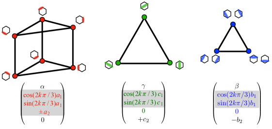
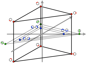
Figure 12: The relation of all of the Gram vectors of $NPA_{1}(\mathcal{Proj})$ for the hexagon. The three different types of singlet projections (nearest neighbor, next nearest, and opposite position) each form either a triangle or a prism shape (left) which could be depicted as the right side figure when all are combined. Although they form a 5-dimensional relation, we project them into lower dimensions for visualization. $k$ in the vector elements label the vertices with $k=0,1,$ and $2$.

The Gram vectors corresponding to all $1+{6\choose 2}=16$ rows/columns of the moment matrix forms a 5-dimensional relation, which is shown in Fig. 12. When we break it down, the Gram vectors for $h_{i,i+1},h_{i,i+2},\text{ and }h_{i,i+3}$ form 3, 2, and 2-dimensional relation respectively as shown on the left side of the figure. Note that the Gram vectors for $h_{i,i+2}$ and $h_{i+3,i+4}$ are exactly the same. All three kinds of Gram vectors combine to form a 5-dimensional relation, but we only show the three-dimensional subspace in the figure (right) for visualization.

The actual values in the coordinates of the Gram vectors are

$$\alpha=\frac{5+\sqrt{13}}{12}\approx 0.717 \beta=\frac{1}{4}(1-3\phi)\approx 0.042 \gamma=\frac{2}{3}(1-2\phi)\approx 0.482$$

$$a_{1}=\frac{1}{6}\sqrt{\frac{1}{2}(5+\phi)}\approx 0.271 b_{1}=\sqrt{\frac{1}{8}(1-3\phi)}\approx 0.145 c_{1}=\frac{1}{3}\sqrt{1+2\phi}\approx 0.416$$ (159)

$$a_{2}=\sqrt{\frac{1}{12}(1+2\phi)}\approx 0.360 b_{2}=\phi/2\approx 0.139 c_{2}=\phi\approx 0.278,$$

where $\phi=1/\sqrt{13}$.

The basis we chose here is the most simplest, which intuitively could be understood in the following way. We choose the Gram vector for the ground state (identity in the moment matrix) to be $(1,0,0,0,0)$ without loss of generality and for simplicity. Then the first coordinate for all of the remaining Gram vectors ($\alpha,\beta$ and $\gamma$) simply correspond to the the expectation value of each kind of projectors. The next three coordinates correspond to the nontrivial prism-shape the $\{h_{i,i+1}\}$s form, and the other Gram vectors happen to follow the same triangular pattern, but without the height dimension. The last coordinate $b_{2}$ and $c_{2}$ could be seen as an additional constant term in order to ensure the normalization $h_{ij}^{2}=h_{ij}$, i.e., each vector must square to become $\alpha,\beta$, and $\gamma$.

Interestingly, the hexagon Hamiltonian admits a decomposition that was used heavily in this study:

$$H=\left(\frac{1}{2}h_{12}+h_{23}+h_{34}+\frac{1}{2}h_{45}\right)+\left(\frac{1}{2}h_{45}+h_{56}+h_{61}+\frac{1}{2}h_{12}\right),$$ (160)

and

$$\lVert H\rVert=\Big{\lVert}\frac{1}{2}h_{12}+h_{23}+h_{34}+\frac{1}{2}h_{45}\Big{\rVert}+\Big{\lVert}\frac{1}{2}h_{45}+h_{56}+h_{61}+\frac{1}{2}h_{12}\Big{\rVert}$$ (161)

simultaneously, however, $NPA_{1}(\mathcal{Proj})$ fails for the decomposed sub-hamiltonians, which is only observed for this particular case. It is quite likely that the $SoS_{1}(\mathcal{Proj})$ for the hexagon becomes severely more complicated than any other $SoS_{1}(\mathcal{Proj})$ we provided in this work.

References

- [Bet31] HA Bethe “Zur Theorie der Metalle, I. Eigenwerte und Eigenfunktionen der linearen Atomkette” In Zeitschrift fur Physik 71, 1931, pp. 205–231
- [LR34] Dudley Ernest Littlewood and Archibald Read Richardson “Group characters and algebra” In Philosophical Transactions of the Royal Society of London. Series A, Containing Papers of a Mathematical or Physical Character 233.721-730 The Royal Society London, 1934, pp. 99–141
- [LM62] Elliott Lieb and Daniel Mattis “Ordering energy levels of interacting spin systems” In Journal of Mathematical Physics 3.4 American Institute of Physics, 1962, pp. 749–751
- [MG69] Chanchal K Majumdar and Dipan K Ghosh “On Next-Nearest-Neighbor Interaction in Linear Chain. I” In Journal of Mathematical Physics 10.8 American Institute of Physics, 1969, pp. 1388–1398
- [TL71] H… Temperley and E.. Lieb “Relations between the ‘percolation’ and ‘colouring’ problem and other graph-theoretical problems associated with regular planar lattices: some exact results for the ‘percolation’ problem” In Proc. Roy. Soc. Lond. A. 322, 1971, pp. 251–280 URL: http://math.bme.hu/~balint/oktatas/perkolacio/percolation_papers/temperley_lieb.pdf
- [Kar72] Richard M. Karp “Reducibility among Combinatorial Problems” In Complexity of Computer Computations: Proceedings of a symposium on the Complexity of Computer Computations, held March 20–22, 1972, at the IBM Thomas J. Watson Research Center, Yorktown Heights, New York, and sponsored by the Office of Naval Research, Mathematics Program, IBM World Trade Corporation, and the IBM Research Mathematical Sciences Department Boston, MA: Springer US, 1972, pp. 85–103 DOI: 10.1007/978-1-4684-2001-2˙9
- [Pro76] Claudio Procesi “The invariant theory of n × n matrices” In Advances in Mathematics 19.3, 1976, pp. 306–381 DOI: https://doi.org/10.1016/0001-8708(76)90027-X
- [SS81] B. Sriram Shastry and Bill Sutherland “Exact ground state of a quantum mechanical antiferromagnet” In Physica B+C 108.1, 1981, pp. 1069–1070 DOI: https://doi.org/10.1016/0378-4363(81)90838-X
- [CP84] Dragos Cvetkovic and Milenko Petric “A table of connected graphs on six vertices” In Discrete Mathematics 50, 1984, pp. 37–49 DOI: https://doi.org/10.1016/0012-365X(84)90033-5
- [GW95] Michel X Goemans and David P Williamson “Improved approximation algorithms for maximum cut and satisfiability problems using semidefinite programming” In Journal of the ACM (JACM) 42.6 ACM New York, NY, USA, 1995, pp. 1115–1145
- [KK00] Akihisa Koga and Norio Kawakami “Quantum Phase Transitions in the Shastry-Sutherland Model for ” In Phys. Rev. Lett. 84 American Physical Society, 2000, pp. 4461–4464 DOI: 10.1103/PhysRevLett.84.4461
- [Gri01] Dima Grigoriev “Linear lower bound on degrees of Positivstellensatz calculus proofs for the parity” In Theoretical Computer Science 259.1, 2001, pp. 613–622 DOI: https://doi.org/10.1016/S0304-3975(00)00157-2
- [Las01] Jean B. Lasserre “Global Optimization with Polynomials and the Problem of Moments” In SIAM Journal on Optimization 11.3, 2001, pp. 796–817 DOI: 10.1137/S1052623400366802
- [Kum02] Brijesh Kumar “Quantum spin models with exact dimer ground states” In Phys. Rev. B 66 American Physical Society, 2002, pp. 024406 DOI: 10.1103/PhysRevB.66.024406
- [Lau03] Monique Laurent “Lower Bound for the Number of Iterations in Semidefinite Hierarchies for the Cut Polytope” In Mathematics of Operations Research 28.4 INFORMS, 2003, pp. 871–883 URL: http://www.jstor.org/stable/4127013
- [Par03] Pablo A Parrilo “Semidefinite programming relaxations for semialgebraic problems” In Mathematical Programming 96.2, 2003, pp. 293–320 DOI: 10.1007/s10107-003-0387-5
- [WB03] Pawel Wocjan and Thomas Beth “The 2-local Hamiltonian problem encompasses NP” In International Journal of Quantum Information 1.03 World Scientific, 2003, pp. 349–357
- [GP04] Karin Gatermann and Pablo A Parrilo “Symmetry groups, semidefinite programs, and sums of squares” In Journal of Pure and Applied Algebra 192.1-3 Elsevier, 2004, pp. 95–128
- [San05] Anders W. Sandvik “Ground State Projection of Quantum Spin Systems in the Valence-Bond Basis” In Phys. Rev. Lett. 95 American Physical Society, 2005, pp. 207203 DOI: 10.1103/PhysRevLett.95.207203
- [BS06] K.S.D. Beach and Anders W. Sandvik “Some formal results for the valence bond basis” In Nuclear Physics B 750.3, 2006, pp. 142–178 DOI: https://doi.org/10.1016/j.nuclphysb.2006.05.032
- [Jam06] Gordon Douglas James “The representation theory of the symmetric groups” Springer, 2006
- [Zuc06] David Zuckerman “Linear degree extractors and the inapproximability of max clique and chromatic number” In Proceedings of the thirty-eighth annual ACM symposium on Theory of computing, 2006, pp. 681–690
- [Kem+07] Julia Kempe, Hirotada Kobayashi, Keiji Matsumoto, Ben Toner and Thomas Vidick “Entangled games are hard to approximate”, 2007 arXiv:0704.2903 [quant-ph]
- [Kho+07] Subhash Khot, Guy Kindler, Elchanan Mossel and Ryan O’Donnell “Optimal inapproximability results for MAX-CUT and other 2-variable CSPs?” In SIAM Journal on Computing 37.1 SIAM, 2007, pp. 319–357
- [Maz07] D.A.(ed.) Mazziotti “Reduced-Density-Matrix Mechanics: With Application to Many- Electron Atoms and Molecules,” In Advances in Chemical Physics 134 New York: Wiley, 2007
- [NPA07] Miguel Navascués, Stefano Pironio and Antonio Acín “Bounding the Set of Quantum Correlations” In Physical Review Letters 98.1 American Physical Society (APS), 2007 DOI: 10.1103/physrevlett.98.010401
- [NPA08] Miguel Navascuès, Stefano Pironio and Antonio Acìn “A convergent hierarchy of semidefinite programs characterizing the set of quantum correlations” In New Journal of Physics 10.7 IOP Publishing, 2008, pp. 073013 DOI: 10.1088/1367-2630/10/7/073013
- [KRT09] Julia Kempe, Oded Regev and Ben Toner “Unique Games with Entangled Provers are Easy”, 2009 arXiv:0710.0655 [quant-ph]
- [Lau09] Monique Laurent “Sums of Squares, Moment Matrices and Optimization Over Polynomials” In Emerging Applications of Algebraic Geometry New York, NY: Springer New York, 2009, pp. 157–270 DOI: 10.1007/978-0-387-09686-5˙7
- [Bea+10] N. Beaudrap, M. Ohliger, T.. Osborne and J. Eisert “Solving Frustration-Free Spin Systems” In Phys. Rev. Lett. 105 American Physical Society, 2010, pp. 060504 DOI: 10.1103/PhysRevLett.105.060504
- [PNA10] S. Pironio, M. Navascués and A. Acìn “Convergent Relaxations of Polynomial Optimization Problems with Noncommuting Variables” In SIAM Journal on Optimization 20.5, 2010, pp. 2157–2180 DOI: 10.1137/090760155
- [San10] Anders W. Sandvik “Computational Studies of Quantum Spin Systems” In AIP Conference Proceedings AIP, 2010 DOI: 10.1063/1.3518900
- [BH12] Thomas Barthel and Robert Hubener “Solving Condensed-Matter Ground-State Problems by Semidefinite Relaxations” In Physical Review Letters 108.20 American Physical Society (APS), 2012 DOI: 10.1103/physrevlett.108.200404
- [BP12] Tillmann Baumgratz and Martin B Plenio “Lower bounds for ground states of condensed matter systems” In New Journal of Physics 14.2 IOP Publishing, 2012, pp. 023027 DOI: 10.1088/1367-2630/14/2/023027
- [FH13] William Fulton and Joe Harris “Representation theory: a first course” Springer Science & Business Media, 2013
- [Bar14] Boaz Barak “Sum of Squares Upper Bounds, Lower Bounds, and Open Questions”, 2014 URL: https://www.boazbarak.org/sos/prev/files/all-notes.pdf
- [BP15] Cedric Bamps and Stefano Pironio “Sum-of-squares decompositions for a family of Clauser-Horne-Shimony-Holt-like inequalities and their application to self-testing” In Physical Review A 91.5 American Physical Society (APS), 2015 DOI: 10.1103/physreva.91.052111
- [BH16] Fernando G… Brandão and Aram W. Harrow “Product-State Approximations to Quantum States” In Communications in Mathematical Physics 342.1, 2016, pp. 47–80 DOI: 10.1007/s00220-016-2575-1
- [Joh+16] Nathaniel Johnston, Rajat Mittal, Vincent Russo and John Watrous “Extended non-local games and monogamy-of-entanglement games” In Proceedings of the Royal Society A: Mathematical, Physical and Engineering Sciences 472.2189 The Royal Society, 2016, pp. 20160003 DOI: 10.1098/rspa.2016.0003
- [Sat+16] Or Sattath, Siddhardh C. Morampudi, Chris R. Laumann and Roderich Moessner “When a local Hamiltonian must be frustration-free” In Proceedings of the National Academy of Sciences 113.23 Proceedings of the National Academy of Sciences, 2016, pp. 6433–6437 DOI: 10.1073/pnas.1519833113
- [Bac+17] Flavio Baccari, Daniel Cavalcanti, Peter Wittek and Antonio Acìn “Efficient device-independent entanglement detection for multipartite systems” In Physical Review X 7.2 APS, 2017, pp. 021042
- [Cha+17] Rui Chao, Ben W. Reichardt, Chris Sutherland and Thomas Vidick “Overlapping Qubits” In 8th Innovations in Theoretical Computer Science Conference (ITCS 2017) 67, Leibniz International Proceedings in Informatics (LIPIcs) Dagstuhl, Germany: Schloss Dagstuhl–Leibniz-Zentrum fuer Informatik, 2017, pp. 48:1–48:21 DOI: 10.4230/LIPIcs.ITCS.2017.48
- [PM17] Stephen Piddock and Ashley Montanaro “The Complexity of Antiferromagnetic Interactions and 2D Lattices” In Quantum Info. Comput. 17.7–8 Paramus, NJ: Rinton Press, Incorporated, 2017, pp. 636–672
- [Ben+18] Adam Bene Watts, Aram W. Harrow, Gurtej Kanwar and Anand Natarajan “Algorithms, Bounds, and Strategies for Entangled XOR Games” Schloss Dagstuhl - Leibniz-Zentrum fuer Informatik GmbH, Wadern/Saarbruecken, Germany, 2018 DOI: 10.4230/LIPICS.ITCS.2019.10
- [Bra+19] Sergey Bravyi, David Gosset, Robert König and Kristan Temme “Approximation algorithms for quantum many-body problems” In Journal of Mathematical Physics 60.3 AIP Publishing LLC, 2019, pp. 032203
- [GP19] Sevag Gharibian and Ojas Parekh “Almost Optimal Classical Approximation Algorithms for a Quantum Generalization of Max-Cut” Schloss Dagstuhl - Leibniz-Zentrum fuer Informatik GmbH, Wadern/Saarbruecken, Germany, 2019 DOI: 10.4230/LIPICS.APPROX-RANDOM.2019.31
- [Lee+19] Jong Yeon Lee, Yi-Zhuang You, Subir Sachdev and Ashvin Vishwanath “Signatures of a Deconfined Phase Transition on the Shastry-Sutherland Lattice: Applications to Quantum Critical ” In Phys. Rev. X 9 American Physical Society, 2019, pp. 041037 DOI: 10.1103/PhysRevX.9.041037
- [Rad19] Louk Rademaker “Exact ground state of the Lieb-Mattis Hamiltonian as a superposition of Néel states” In Phys. Rev. Res. 1 American Physical Society, 2019, pp. 032018 DOI: 10.1103/PhysRevResearch.1.032018
- [AGM20] Anurag Anshu, David Gosset and Karen Morenz “Beyond Product State Approximations for a Quantum Analogue of Max Cut” Schloss Dagstuhl - Leibniz-Zentrum für Informatik, 2020 DOI: 10.4230/LIPICS.TQC.2020.7
- [Cui+20] David Cui, Arthur Mehta, Hamoon Mousavi and Seyed Sajjad Nezhadi “A generalization of CHSH and the algebraic structure of optimal strategies” In Quantum 4 Verein zur Forderung des Open Access Publizierens in den Quantenwissenschaften, 2020, pp. 346 DOI: 10.22331/q-2020-10-21-346
- [HKR20] Arbel Haim, Richard Kueng and Gil Refael “Variational-Correlations Approach to Quantum Many-body Problems”, 2020 arXiv:2001.06510 [cond-mat.str-el]
- [IR21] Marie Ioannou and Denis Rosset “Noncommutative polynomial optimization under symmetry” In arXiv preprint arXiv:2112.10803, 2021
- [KL21] Yuehaw Khoo and Michael Lindsey “Scalable semidefinite programming approach to variational embedding for quantum many-body problems”, 2021 arXiv:2106.02682 [math.OC]
- [PT21] Ojas Parekh and Kevin Thompson “Application of the Level-2 Quantum Lasserre Hierarchy in Quantum Approximation Algorithms” Schloss Dagstuhl - Leibniz-Zentrum für Informatik, 2021 DOI: 10.4230/LIPICS.ICALP.2021.102
- [PT21a] Ojas Parekh and Kevin Thompson “Beating Random Assignment for Approximating Quantum 2-Local Hamiltonian Problems” In 29th Annual European Symposium on Algorithms (ESA 2021) 204, Leibniz International Proceedings in Informatics (LIPIcs) Dagstuhl, Germany: Schloss Dagstuhl – Leibniz-Zentrum für Informatik, 2021, pp. 74:1–74:18 DOI: 10.4230/LIPIcs.ESA.2021.74
- [Pro21] C Procesi “A note on the Formanek Weingartn function” In Note di Matematica 41, 2021 URL: http://siba-ese.unisalento.it/index.php/notemat/article/view/24154
- [WKS21] Jurriaan Wouters, Hosho Katsura and Dirk Schuricht “Interrelations among frustration-free models via Witten’s conjugation” In SciPost Phys. Core 4 SciPost, 2021, pp. 027 DOI: 10.21468/SciPostPhysCore.4.4.027
- [AAG22] Anurag Anshu, Itai Arad and David Gosset “An Area Law for 2d Frustration-Free Spin Systems” In Proceedings of the 54th Annual ACM SIGACT Symposium on Theory of Computing, STOC 2022 Rome, Italy: Association for Computing Machinery, 2022, pp. 12–18 DOI: 10.1145/3519935.3519962
- [GMZ22] David Gamarnik, Cristopher Moore and Lenka Zdeborova “Disordered systems insights on computational hardness” In Journal of Statistical Mechanics: Theory and Experiment 2022.11 IOP PublishingSISSA, 2022, pp. 114015 DOI: 10.1088/1742-5468/ac9cc8
- [Has22] Matthew B Hastings “Perturbation Theory and the Sum of Squares” In arXiv preprint arXiv: 2205.12325, 2022
- [HO22] Matthew B. Hastings and Ryan O’Donnell “Optimizing Strongly Interacting Fermionic Hamiltonians”, 2022 arXiv:2110.10701 [quant-ph]
- [Hwa+22] Yeongwoo Hwang, Joe Neeman, Ojas Parekh, Kevin Thompson and John Wright “Unique Games hardness of Quantum Max-Cut, and a conjectured vector-valued Borell’s inequality”, 2022 arXiv:2111.01254 [quant-ph]
- [Hwa+22a] Yeongwoo Hwang, Ojas Parekh, Kevin Thompson and John Wright, personal communication, 2022
- [Ji+22] Zhengfeng Ji, Anand Natarajan, Thomas Vidick, John Wright and Henry Yuen “MIP*=RE”, 2022 arXiv:2001.04383 [quant-ph]
- [Kin22] Robbie King “An Improved Approximation Algorithm for Quantum Max-Cut” In arXiv preprint arXiv:2209.02589, 2022
- [KM22] Dmitriy Kunisky and Cristopher Moore “The spectrum of the Grigoriev-Laurent pseudomoments”, 2022 arXiv:2203.05693 [math.OC]
- [Lee22] Eunou Lee “Optimizing quantum circuit parameters via SDP” In arXiv preprint arXiv: 2209.00789, 2022
- [PT22] Ojas Parekh and Kevin Thompson “An Optimal Product-State Approximation for 2-Local Quantum Hamiltonians with Positive Terms”, 2022 arXiv:2206.08342 [quant-ph]
- [YSW22] Jianwei Yang, Anders W. Sandvik and Ling Wang “Quantum criticality and spin liquid phase in the Shastry-Sutherland model” In Phys. Rev. B 105 American Physical Society, 2022, pp. L060409 DOI: 10.1103/PhysRevB.105.L060409
- [ApS23] MOSEK ApS “MOSEK Fusion API for Python manual. Version 10.0.”, 2023 URL: https://docs.mosek.com/latest/pythonfusion/index.html
- [Gho23] Pratyay Ghosh “Exact quantum ground state of a two-dimensional quasicrystalline antiferromagnet” arXiv, 2023 DOI: 10.48550/ARXIV.2301.11331
- [Sac23] Subir Sachdev “Quantum Phases of Matter” Cambridge University Press, 2023
- [Wat+23] Adam Bene Watts, Anirban Chowdhury, Aidan Epperly, J William Helton and Igor Klep “Relaxations and Exact Solutions to Quantum Max Cut via the Algebraic Structure of Swap Operators” In arXiv preprint arXiv:2307.15661, 2023
C13 \missingM99