A Continuous-Time Dynamic Factor Model for Intensive Longitudinal Data Arising from Mobile Health Studies

Abstract

Intensive longitudinal data (ILD) collected in mobile health (mHealth) studies contain rich information on multiple outcomes measured frequently over time that have the potential to capture short-term and long-term dynamics. Motivated by an mHealth study of smoking cessation in which participants self-report the intensity of many emotions multiple times per day, we describe a dynamic factor model that summarizes the ILD as a low-dimensional, interpretable latent process. This model consists of two submodels: (i) a measurement submodel—a factor model—that summarizes the multivariate longitudinal outcome as lower-dimensional latent variables and (ii) a structural submodel—an Ornstein-Uhlenbeck (OU) stochastic process—that captures the temporal dynamics of the multivariate latent process in continuous time. We derive a closed-form likelihood for the marginal distribution of the outcome and the computationally-simpler sparse precision matrix for the OU process. We propose a block coordinate descent algorithm for estimation. Finally, we apply our method to the mHealth data to summarize the dynamics of 18 different emotions as two latent processes. These latent processes are interpreted by behavioral scientists as the psychological constructs of positive and negative affect and are key in understanding vulnerability to lapsing back to tobacco use among smokers attempting to quit.

1 Introduction

Intensive longitudinal data (ILD) can capture rapid changes in outcomes over time. In mobile health (mHealth) studies, information about multiple longitudinal outcomes is often collected with the aim of understanding the temporal dynamics of unobservable constructs related to mental or physical health. Our work is motivated by an mHealth study of smoking cessation in which the intensity of emotions over time was collected from current smokers attempting to quit. Participants self-reported the intensity of 18 different emotions up to four times per day over 10 days, resulting in a substantial quantity of rich data. For smoking cessation researchers, understanding the temporal dynamics of the latent psychological states that underlie these emotions is of scientific interest.

The volume and complexity of ILD, however, make them challenging to analyze since longitudinal outcomes are often measured irregularly across many individuals; thus statistical methods must be able to handle the high volume of irregularly spaced data. At the same time, the frequent measurements in ILD create many opportunities to discover new information, particularly if the latent constructs of interest vary rapidly. We present a dynamic factor model that is motivated by the need to model multiple longitudinal outcomes measured frequently over time in a flexible yet interpretable manner. Our proposed model consists of two submodels: (i) a measurement submodel—a factor model—that summarizes the multiple observed longitudinal outcomes as lower-dimensional latent factors and (ii) a structural submodel—an Ornstein-Uhlenbeck (OU) stochastic process—that captures the evolution of the multiple correlated latent factors over time. Together, these components of our dynamic factor model are flexible enough to capture the variability in the longitudinal outcomes while avoiding use of a non-parametric or other many-parameter model that inhibits interpretability. In addition to improving interpretability, the low-dimensional nature of the structural submodel also greatly reduces computational complexity, as opposed to fitting a high-dimensional stochastic process directly to the observed outcomes.

One standard approach to modeling changes in multiple correlated longitudinal variables over time is to use an autoregressive (AR) model. These models, which are called vector autoregressive (VAR) models when data are multivariate, have been widely used to model observed outcomes as well as latent variables. For example, Dunson (2003), Cui and Dunson (2014), and Tran et al. (2019) have proposed related methods in which observed longitudinal outcomes are summarized as time-varying lower-dimensional latent variables. The correlation of these latent variables is then modeled with AR or VAR processes. VAR models, however, are specified for balanced data. This situation is often not realistic in the case of ILD, which generally consists of irregularly-measured outcomes, and can lead to biased estimates in cases where the assumption is made but does not hold.

Mixed models have been proposed as alternatives to discrete-time processes for modeling the evolution of latent variables over time and have been previously used in combination with factor models. Unlike the AR and VAR processes, mixed models do not require balanced data. Existing work has focused both on the development of mixed models for modeling the evolution of a single latent factor over time (e.g., Roy and Lin, 2000; Proust et al., 2006; Proust-Lima, Amieva, and Jacqmin-Gadda, 2013) or multiple latent factors (e.g., Liu et al., 2019; Wang, Berger, and Burdick, 2013). Overall, these mixed model-based approaches are useful tools for capturing smooth trends in latent factors. In our application, however, we aim to develop a method that can capture the correlation between and rapid variation in multiple latent emotional constructs over time.

The OU process, which can be thought of as a continuous-time analog of the AR or VAR process, is a stochastic process well-suited for capturing rapid variations over time. Existing work has frequently focused on using the OU process or integrated OU process to model longitudinal outcomes that have been directly observed (or observed with measurement error); e.g., Taylor, Cumberland, and Sy (1994); Sy, Taylor, and Cumberland (1997); Oravecz, Tuerlinckx, and Vandekerckhove (2009); Oravecz, Tuerlinckx, and Vandekerckhove (2016).

In more recent work, the OU process has also been used in the context of latent variable models. Tran et al. (2021a) propose a latent linear mixed model that summarizes multiple observed longitudinal outcomes as a smaller number of latent factors while accounting for the serial correlation between repeated measurements over time via an OU process. This work differs from ours, however, in that the fixed effects that capture the association between the observed covariates and the latent factors are of primary interest; the OU process is incorporated into the structural mixed model as a tool for accounting for serial correlation between repeated observations.

Most closely related to our proposed approach is work by Tran et al. (2021b). Like us, they propose a longitudinal latent variable model that consists of two parts: a measurement submodel to summarize observed outcomes as lower dimensional latent factors and an OU process as the structural submodel for the latent factors. While we differ in the exact specification of the measurement submodel, our chosen models are related. Key distinctions between this existing work and the approach presented in this manuscript are in the model parameterization and computational approach. Tran et al. (2021b) take a Bayesian approach, which requires sampling values of the latent process at each measurement occasion. In the ILD setting, we need approaches that can scale to large numbers of repeated measurements. Here, we choose to work in the frequentist framework. As a result of taking a maximum likelihood-based approach, we can directly maximize the marginal log-likelihood of the observed longitudinal outcome. Furthermore, this framework enables us to employ various algebraic and computational strategies to make estimation faster, resulting in a method more suitable for ILD.

In this work, we fill a gap in the existing literature by proposing an Ornstein-Uhlenbeck factor (OUF) model that captures the temporal dynamics between rapidly-varying correlated latent factors observed via multiple longitudinal outcomes and an estimation algorithm with the computational efficiency to handle ILD. Our novel contributions include (i) a closed-form likelihood for the marginal distribution of the observed outcome, (ii) the derivation of the computationally-simpler sparse precision matrix for the multivariate OU process, (iii) identifiability constraints imposed via scaling constants, and (iv) a block coordinate descent algorithm for estimation and inference in a maximum likelihood framework.

The remainder of this paper is organized as such: In Section 2, we describe the motivating mHealth data; in Section 3, we present our novel method and contributions; in Section 4, we demonstrate the performance of our method via simulation; in Section 5, we illustrate our model via a scientifically–meaningful application to mHealth data; and in Section 6, we provide a discussion.

2 Motivating data

Data motivating this work come from an mHealth study of smoking cessation (Potter et al., 2023). In this observational study, current smokers (N = 218) who were attempting to quit were followed for 10 days. During these 10 days, ecological momentary assessments (EMAs), which enable repeated sampling of individuals’ current states and contexts in real time, were used to track participants’ emotions as they were experienced in a high-frequency manner. Specifically, participants were prompted to respond to a series of questions sent to their smartphones multiple per day at random occasions; the original study design intended for individuals to receive up to four EMAs per day. The EMAs contained a set of questions that assessed the current intensity of multiple emotions measured on a 5-point Likert scale. We focus on a set of 18 emotions consisting of both positive and negative emotions that attempts to capture the distinct-but-correlated underlying emotional states of positive and negative affect (i.e., summary measures of overall positive and negative feeling). The resulting data contain frequent measurements of a substantial number of longitudinal outcomes, where the number of measurement occasions per person ranges from 2 to 47 (mean = 17). Note that these data are only the subset of the full study data that were available at the time of drafting this manuscript. Additional details on the study procedures can be found in Potter et al. (2023). The high rate of measurement enables us to capture rapid changes in emotions over time. To illustrate the dynamics of these responses, Figure 1 shows the responses to emotion-related EMA questions over time for one participant in the study. Understanding the dynamics of smokers’ latent emotional states that underlie the measured responses is of scientific interest among smoking cessation researchers and behavioral scientists more broadly.

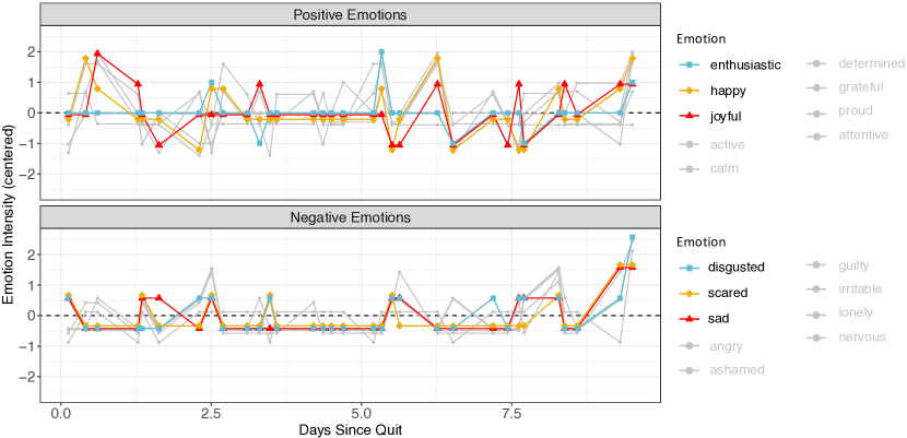
Figure 1: Responses to emotion-related questions over time for one participant in the mHealth study. In this plot, a subset of three positive emotions and three negative emotions are highlighted solely for illustrative purposes; all 18 emotions are later included in the model described in Section 5. Note the rapid fluctuations of these longitudinal outcomes over time.

3 Methods

In this section, we present the OUF model that jointly models multiple observed longitudinal outcomes and the lower dimensional latent factors assumed to generate the observed longitudinal outcomes. Our proposed model consists of two submodels: a measurement submodel and a structural submodel.

3.1 Measurement submodel

Let $\bm{Y}_{i}(t)=[Y_{i1}(t),Y_{i2}(t),...,Y_{iK}(t)]^{\top}$ be a $K\times 1$ vector of measured longitudinal outcomes for individual $i,i=1,...,N$, at time $t$. Assume that individual $i$ has longitudinal outcomes measured at $n_{i}$ occasions. Using the measurement submodel, we model the observed longitudinal outcome $\bm{Y}_{i}(t)$ as

$$\bm{Y}_{i}(t)=\bm{\Lambda}\bm{\eta}_{i}(t)+\bm{u}_{i}+\bm{\epsilon}_{i}(t)$$ (1)

where $\bm{\eta}_{i}(t)$ is a vector of $p$ time-varying latent factors (where $p<K$); $\bm{\Lambda}$ is a $K\times p$-dimensional time-invariant loadings matrix with elements $\lambda_{k,j}$ that captures the degree of association between the latent factors and observed longitudinal outcomes; $\bm{u}_{i}\sim N(0,\bm{\Sigma}_{u})$ is a vector of length $K$ of random intercepts; and $\bm{\epsilon}_{i}(t)\sim N(0,\bm{\Sigma}_{\epsilon})$ is a vector representing measurement error, where $\bm{\Sigma}_{\epsilon}$ is assumed to be a diagonal matrix.

This model builds upon a standard factor model but also includes (i) a random intercept and (ii) a multivariate model for the evolution of the correlated latent processes $\bm{\eta}_{i}(t)$ (described in Section 3.2). We assume that $\bm{\Sigma}_{u}$ is diagonal, as we include this term to account for the longitudinal correlation in the repeated measurements but then model the correlated change in outcomes through the structural submodel. Allowing a non-diagonal $\bm{\Sigma}_{u}$ is possible, but we opt not to do so to avoid the substantial increase computational cost associated with estimation of these extra parameters. We also assume that $\bm{\Lambda}$ contains many structural zeros such that each row of the loadings matrix contains only one non-zero element; this structure means that each observed outcome is a measurement of only a single underlying latent factor. The decision to incorporate structural zeros in the loadings matrix is supported by behavioral science concepts (i.e., Positive and Negative Affect Schedule; PANAS (Watson, Clark, and Tellegen, 1988)), which classify a given emotion as a measurement of a specific category of emotional state. Learning the location of the structural zeros, rather than pre-specifying them, is a possible direction for future work.

3.2 Structural submodel

The structural submodel captures the evolution of the latent factors, $\bm{\eta}_{i}(t)$, over time. We use a multivariate OU process, which can be understood as a continuous-time analog of a VAR process and has the ability to capture rapid temporal variation. Here, we assume a bivariate OU process ($p=2$) for illustrative purposes. The stochastic differential equation definition of the bivariate OU process is

$$d\begin{bmatrix}\eta_{i1}(t)\\ \eta_{i2}(t)\end{bmatrix}=-\underbrace{\begin{bmatrix}\theta_{11}&\theta_{12}\\ \theta_{21}&\theta_{22}\end{bmatrix}}_{\coloneqq\bm{\theta}}\begin{bmatrix}\eta_{i1}(t)\\ \eta_{i2}(t)\end{bmatrix}dt+\underbrace{\begin{bmatrix}\sigma_{11}&0\\ 0&\sigma_{22}\end{bmatrix}}_{\coloneqq\bm{\sigma}}d\begin{bmatrix}W_{i1}(t)\\ W_{i2}(t)\end{bmatrix}$$ (2)

where the diagonal elements of matrix $\bm{\theta}$ capture the mean-reverting tendency of the latent factors (where the mean is assumed to be $0$) and the off-diagonal elements of $\bm{\theta}$ capture correlation between the latent factors. The diagonal elements of $\bm{\theta}$ are required to be positive. The matrix $\bm{\sigma}$, with elements $\sigma_{11}$ and $\sigma_{22}>0$, describes the volatility of the process, where $W_{i1}(t)$ and $W_{i2}(t)$ are both standard Brownian motion. In general, the standard definition of the OU process allows $\bm{\sigma}$ to take non-zero values in the off-diagonal. By restricting $\bm{\sigma}$ to be a simpler diagonal matrix here, we consider the Brownian motion terms as separate noise processes for each latent variable and thus capture all correlation between the latent processes through the $\bm{\theta}$ matrix. We also require that all eigenvalues of the $\bm{\theta}$ matrix have a positive real part; this constraint ensures a mean-reverting process (see Vatiwutipong and Phewchean (2019)).

The multivariate stochastic process provides advantages over a simpler univariate stochastic process as it captures correlation between multiple variables over time; however, the multivariate nature does increase the complexity of the model and thus the computational burden. We address this complexity in the next section.

3.2.1 Marginal covariance and precision matrices for the OU process

Rather than taking a Bayesian strategy or relying on the complete-data likelihood and taking an expectation-maximization (EM) approach to estimation, we directly maximize the likelihood of the observed data. Direct maximization of the marginal likelihood allows us to avoid repeatedly calculating values of the latent factors at each measurement occasion (via posterior sampling in a Bayesian framework or via complex integrals in the E-step of the EM algorithm). Thus, our approach is more scalable to the ILD setting.

In order to carry out our estimation algorithm (described in Section 3.5), we require the marginal covariance matrix of the OU process. Vatiwutipong and Phewchean (2019) present a form of the conditional variance and cross-covariance function for the OU process but provide these functions in integral forms that are not amenable to likelihood-based inference. To avoid approximations resulting from numerical integration, (i) we derive an analytic form of the conditional covariance function and (ii) we account for the additional uncertainty of an unknown initial state by deriving the analytic form of the marginal covariance function. For a stationary OU process with known initial state at time $t_{0}=0$, $\bm{\eta}(t_{0})$, the conditional mean at time $t$ is $\mathbb{E}\{\bm{\eta}(t)|\bm{\eta}(t_{0})\}=e^{-\bm{\theta}t}\bm{\eta}(t_{0})$. Assuming a marginal mean of 0, the conditional and marginal covariance functions follow:

Lemma 3.1

The analytic form of the OU conditional covariance at times $s$ and $t$, where $s\leq t$, is

$$Cov\{\eta(s),\eta(t)|\eta(t_{0}=0)\} =vec^{-1}\Big{\{}(\theta\oplus\theta)^{-1}\big{[}e^{s(\theta\oplus\theta)}-I\big{]}e^{-[t\theta\oplus s\theta]}vec\{\sigma\sigma^{\top}\}\Big{\}}$$

Lemma 3.2

The analytic form of the OU marginal covariance at times $s$ and $t$, $s\leq t$, is

$$Cov\{\eta(s),\eta(t)\}=vec^{-1}\Big{\{}(\theta\oplus\theta)^{-1}\big{[}e^{(\theta\oplus\theta)s-(\theta t\oplus\theta s)}\big{]}vec\{\sigma\sigma^{\top}\}\Big{\}}$$

Here, $\oplus$ denotes the Kronecker sum, defined for square matrices $\bm{A}$ and $\bm{B}$ of sizes $a$ and $b$, respectively, as $\bm{A}\oplus\bm{B}=\bm{A}\otimes\bm{I}_{b}+\bm{I}_{a}\otimes\bm{B}$; and the $vec\{\bm{A}\}$ operation consists of stacking the columns of matrix $\bm{A}$ into a column vector. For details on the derivations of these results, see Section A.1 and A.2 of the supplementary material.

In addition to the marginal covariance function of the OU process, we derive the precision matrix. Due to the Markov property of the OU process, the precision matrix is block tri-diagonal and thus much simpler to calculate than the dense covariance matrix.

Lemma 3.3

Let $\bm{\Omega}$ be the precision matrix of the OU process observed at $n$ occasions and define the stationary variance as $\bm{V}:=vec^{-1}\big{\{}(\bm{\theta}\oplus\bm{\theta})^{-1}vec\{\bm{\sigma}\bm{\sigma}^{\top}\}\big{\}}$. Then $\bm{\Omega}$ has the structure

$$\bm{\Omega}=\begin{bmatrix}\bm{\Omega}_{11}&\bm{\Omega}_{12}&0&\cdots&0\\ \bm{\Omega}_{12}^{\top}&\bm{\Omega}_{22}&\bm{\Omega}_{23}&\cdots&0\\ 0&\bm{\Omega}_{23}^{\top}&\bm{\Omega}_{33}&\ddots&\vdots\\ \vdots&\vdots&\ddots&\ddots&\bm{\Omega}_{n-1,n}\\ 0&0&\cdots&\bm{\Omega}_{n-1,n}^{\top}&\bm{\Omega}_{nn}\\ \end{bmatrix}$$ (3)

and each block indexed by $j$ for $1<j<n$ in the tri-diagonal matrix is

$$\bm{\Omega}_{11}=\big{[}\bm{V}-\bm{V}e^{-\bm{\theta}^{\top}(t_{2}-t_{1})}\bm{V}^{-1}e^{-\bm{\theta}(t_{2}-t_{1})}\bm{V}\big{]}^{-1}$$ (4)

$$\bm{\Omega}_{j,j+1}=-\big{[}\bm{V}-\bm{V}e^{-\bm{\theta}^{\top}(t_{j+1}-t_{j})}\bm{V}^{-1}e^{-\bm{\theta}(t_{j+1}-t_{j})}\bm{V}\big{]}^{-1}\bm{V}e^{-\bm{\theta}^{\top}(t_{j+1}-t_{j})}\bm{V}^{-1}$$

$$\bm{\Omega}_{jj}=\bm{V}^{-1}+\bm{V}^{-1}e^{-\bm{\theta}(t_{j}-t_{j-1})}\bm{V}\big{[}\bm{V}-\bm{V}e^{-\bm{\theta}^{\top}(t_{j}-t_{j-1})}\bm{V}^{-1}e^{-\bm{\theta}(t_{j}-t_{j-1})}\bm{V}\big{]}^{-1}\bm{V}e^{-\bm{\theta}^{\top}(t_{j}-t_{j-1})}\bm{V}^{-1}$$

$$\hskip 25.6073pt+\big{[}\bm{V}-\bm{V}e^{-\bm{\theta}^{\top}(t_{j+1}-t_{j})}\bm{V}^{-1}e^{-\bm{\theta}(t_{j+1}-t_{j})}\bm{V}\big{]}^{-1}\bm{V}e^{-\bm{\theta}^{\top}(t_{j+1}-t_{j})}\bm{V}^{-1}e^{-\bm{\theta}(t_{j+1}-t_{j})}$$

$$\bm{\Omega}_{nn}=\bm{V}^{-1}+\bm{V}^{-1}e^{-\bm{\theta}(t_{n}-t_{n-1})}\bm{V}\big{[}\bm{V}-\bm{V}e^{-\bm{\theta}^{\top}(t_{n}-t_{n-1})}\bm{V}^{-1}e^{-\bm{\theta}(t_{n}-t_{n-1})}\bm{V}\big{]}^{-1}\bm{V}e^{-\bm{\theta}^{\top}(t_{n}-t_{n-1})}\bm{V}^{-1}$$

The derivation for each block is given in Section A.3 of the supplementary material. Later, during estimation, we take advantage of the sparse precision matrix to simplify computation. This sparsity becomes particularly advantageous as the number of individuals and observations per individual in a dataset increase.

3.3 Joint distribution and likelihood

Together, the measurement and structural submodels imply that the observed longitudinal outcomes are normally distributed with mean 0 and covariance $\bm{\Sigma}_{i}^{*}:=Var(\bm{Y}_{i})=(\bm{I}_{n_{i}}\otimes\bm{\Lambda})Var(\bm{\eta}_{i})(\bm{I}_{n_{i}}\otimes\bm{\Lambda})^{\top}+\bm{J}_{n_{i}}\otimes\bm{\Sigma}_{u}+\bm{I}_{n_{i}}\otimes\bm{\Sigma}_{\epsilon}$, where $\bm{I}_{n_{i}}$ is an $n_{i}\times n_{i}$ identity matrix and $\bm{J}_{n_{i}}$ is an $n_{i}\times n_{i}$ matrix of ones. We estimate the OUF model by minimizing the following function, which equal to twice the negative log-likelihood up to a constant: $-2logL(\bm{Y})=\sum_{i=1}^{N}log|\bm{\Sigma}_{i}^{*}|+\sum_{i=1}^{N}\bm{Y}_{i}^{\top}\bm{\Sigma}_{i}^{*-1}\bm{Y}_{i}$.

3.4 Identification issues

Before fitting our model, we must make additional assumptions to address identifiability issues common to factor models. Because both $\bm{\Lambda}$ and $\bm{\eta}_{i}(t)$ are unknown, multiplying $\bm{\Lambda}$ by some matrix, say $\bm{A}$, and multiplying $\bm{\eta}_{i}(t)$ by $\bm{A}^{-1}$ will result in the same model. To make a factor model identifiable, constraints must be placed on either the loadings matrix or the latent factors. Aguilar and West (2000) and Carvalho et al. (2008), for example, make the standard assumption of requiring the loadings matrix to be triangular while Tran et al. (2019), for example, fix the variance of the latent factors at 1. We also fix the scale of the latent factors but propose a novel approach for doing so. Letting $\bm{\eta}_{i}$ be the $(p\times n_{i})$-length vector of latent variables values stacked over measurement occasions, we constrain $Var(\bm{\eta}_{i})$ to have diagonal elements equal to 1. This constraint means that the OU process must have a stationary variance equal to 1. By fixing the scale of the latent factors, we can allow the elements of the loadings matrix $\bm{\Lambda}$ to vary almost freely during estimation. For a generic $\bm{\Lambda}$ (without structural zeros), the only constraint on the loadings matrix is that the sign of the first element must be positive. Together these constraints make our model identifiable; the constraint on the OU process identifies the scale and the constraint on the first element of the loadings matrix identifies the direction. Because we later make the simplifying assumption that $\bm{\Lambda}$ contains structural zeros with a single non-zero loading per row, flipping the signs on both the loadings and the latent factors results in the same model; we choose to keep the signs that correspond to the most relevant interpretation of the model given the application. Another constraint could be added to require that one loading per column of $\bm{\Lambda}$ is positive; this would avoid sign flipping. We revisit our approach to selecting the correct sign later in the context of rescaling the OU process.

To impose this identifiability constraint, we use a set of $p$ constants to re-scale the OU process parameters. We summarize this identifiability constraint for the bivariate OU process as:

Lemma 3.4

Using a pair of positive scalar constants $c_{1}$ and $c_{2}$, we can re-scale an arbitrary OU process parameterized by $\bm{\theta}$ and $\bm{\sigma}$ to have stationary variance of 1, where this re-scaled OU process is parameterized by $\bm{\theta}^{*}$ and $\bm{\sigma}^{*}$ according to

$$\begin{bmatrix}\theta^{*}_{11}&\theta^{*}_{12}\\ \theta^{*}_{21}&\theta^{*}_{22}\end{bmatrix}=\begin{bmatrix}\theta_{11}&\frac{c_{1}}{c_{2}}\theta_{12}\\ \frac{c_{2}}{c_{1}}\theta_{21}&\theta_{22}\end{bmatrix}\text{ and }\begin{bmatrix}\sigma^{*}_{11}&0\\ 0&\sigma^{*}_{22}\end{bmatrix}=\begin{bmatrix}c_{1}\sigma_{11}&0\\ 0&c_{2}\sigma_{22}\end{bmatrix}$$ (5)

In Section A.4 of the supplementary material, we show why this re-scaling approach works for any mean-reverting OU process. This constraint can also be extended to OU processes of higher dimensions.

Although this identifiability assumption allows us to identify the magnitude of the loadings in the factor model, it does so only up to a sign change. Consider again the case of a bivariate OU process. The likelihood for our model is equivalent for pairs of scaling constants $(c_{1}=1,c_{2}=1)$ and $(c_{1}=1,c_{2}=-1)$. In practice, the model would be the same under both pairs of scaling constants (and so we restrict $c_{1}$ and $c_{2}$ to be positive during estimation) but interpretation of model parameters would differ. After estimation, the signs on estimated model parameters can easily be flipped to match the most relevant interpretation of the data by multiplying estimates of $\bm{\Lambda}$ and $\bm{\theta}$ by a $p\times p$ matrix with the constants along the diagonal.

3.5 Estimation algorithm

To fit this model, we take an iterative approach to estimation in which we directly maximize the marginal likelihood of our observed longitudinal outcome using a block coordinate descent algorithm and rely on simpler existing models to inform the initial parameter estimates. In the block coordinate descent algorithm, we split parameters into two different blocks: one block for parameters in the measurement submodel ($\bm{\Lambda}$, $\bm{\Sigma}_{u}$, $\bm{\Sigma}_{\epsilon}$) and the other for parameters in the structural submodel ($\bm{\theta}$, $\bm{\sigma}$). Note that each element of these blocks is actually a matrix of parameters. Within each block-wise iteration, we minimize the log-likelihood with respect to one block of parameters, given the current estimates of the other block of parameters, using Newton algorithms as implemented in R’s stats package (R Core Team, 2022). By updating parameters in blocks, we can leverage the availability of analytic gradients for parameters in the measurement submodel. The Kronecker structure of the covariance matrix for each individual’s longitudinal outcomes $\bm{Y}_{i}$ allows us to derive these analytic gradients. We present the general structure of the gradient here:

Lemma 3.5

The gradient of the log-likelihood for a single individual with respect to one of the measurement submodel parameters, $\Theta_{j}$, has the general form

$$\frac{\partial logL(\bm{Y}_{i})}{\partial\Theta_{j}}=-\frac{1}{2}\Bigg{[}tr\Bigg{\{}\Big{(}I-\bm{\Sigma}_{i}^{*-1}\bm{Y}_{i}\bm{Y}_{i}^{\top}\Big{)}\Sigma_{i}^{*-1}\frac{\partial\bm{\Sigma}_{i}^{*}}{\partial\Theta_{j}}\Bigg{\}}\Bigg{]}$$

where the exact form of $\frac{\partial\bm{\Sigma}_{i}^{*}}{\partial\Theta_{j}}$ depends on the specific parameter; either $\lambda_{k}$, $\sigma_{u_{k}}$, or $\sigma_{\epsilon_{k}}$.

The complete set of analytic gradients is given in Section A.5 of the supplementary material. The computational advantage of using the analytic gradient, as opposed to a numerical approach to differentiation, is particularly notable as the number of longitudinal outcomes—and thus parameters in the measurement submodel—increases.

Prior to maximizing the marginal likelihood, we use a cross-sectional factor model to initialize $\bm{\Lambda}$, $\bm{\theta}$, and $\bm{\sigma}$, and use linear mixed models to initialize $\bm{\Sigma}_{u}$ and $\bm{\Sigma}_{\epsilon}$. Then, we iteratively update parameter estimates using the following block coordinate descent algorithm:

1. Initialize estimates of $\bm{\Lambda}^{(0)},\bm{\Sigma}_{u}^{(0)},\bm{\Sigma}_{\epsilon}^{(0)},\bm{\theta}^{(0)},\bm{\sigma}^{(0)}$. Measurement submodel parameters are always initialized empirically; for structural submodel parameters, two sets of initial estimates are considered—an empirical set of values estimated from cross-sectional factor scores and a default set of values. The set of values that corresponds to the higher log-likelihood given the current data is used.

2. Set iteration index $r=1$ and convergence indicator $\delta=0$. While $\delta=0$,

   1. Update block 1 (measurement submodel):

      $$\bm{\Lambda}^{(r)},\bm{\Sigma}_{u}^{(r)},\bm{\Sigma}_{\epsilon}^{(r)}=\underset{\bm{\Lambda},\bm{\Sigma}_{u},\bm{\Sigma}_{\epsilon}}{argmax}\big{\{}logL(\bm{\Lambda},\bm{\Sigma}_{u},\bm{\Sigma}_{\epsilon}|Y;\bm{\theta}^{(r-1)},\bm{\sigma}^{(r-1))})\big{\}}.$$

      Maximization is done via a Newton-type algorithm using analytic gradients (Lemma 3.5).

   2. Update block 2 (structural submodel):

      $$\bm{\theta}^{(r)},\bm{\sigma}^{(r)}=\underset{\bm{\theta},\bm{\sigma}}{argmax}\big{\{}logL(\bm{\theta},\bm{\sigma}|Y;\bm{\Lambda}^{(r)},\bm{\Sigma}_{u}^{(r)},\bm{\Sigma}_{\epsilon}^{(r)})\big{\}}.$$

      Maximization is done via a quasi-Newton algorithm using numerical gradients.

   3. Using Lemma 3.4, re-scale OU parameters to satisfy the identifiability constraint.

   4. Check for block-wise convergence: Let $\bm{\Theta}$ be a vector containing all elements of $\bm{\Lambda}$, $\bm{\Sigma}_{u}$, $\bm{\Sigma}_{\epsilon}$, $\bm{\theta}$, and $\bm{\sigma}$. Then, calculate

      $$\delta=\max\Big{\{}I\big{\{}|\bm{\Theta}^{(r)}-\bm{\Theta}^{(r-1)}|/\bm{\Theta}^{(r)}<10^{-6}\big{\}},\ I\big{\{}logL(\bm{\Theta}^{(r)}|\bm{Y})-logL(\bm{\Theta}^{(r-1)}|\bm{Y})<10^{-6}\big{\}}\Big{\}}$$

      where all operations on $\bm{\Theta}$ are element-wise.

   5. Update $r$: $r=r+1$

3. Estimate Fisher Information-based standard errors from a numerical approximation to the Hessian of the log-likelihood, $\frac{\partial^{2}}{\partial\Theta\partial\Theta^{\top}}logL(\bm{\Lambda}^{(r)},\bm{\Sigma}_{u}^{(r)},\bm{\Sigma}_{\epsilon}^{(r)},\bm{\theta}^{(r)}|Y).$

Note that when estimating standard errors, the parameterization of the likelihood differs slightly: the likelihood now depends on only one of the parameter matrices in the structural submodel, $\bm{\theta}$, and not the other, $\bm{\sigma}$. This change in parameterization is a result of the identifiability constraint that is placed on the stationary variance of the OU process. Since we are no longer conditioning on fixed measurement submodel parameters in this step, we restrict $\bm{\sigma}$ to be a function of $\bm{\theta}$, where this function is derived from the identifiability constraint; thus, the likelihood is not over-parameterized. Standard error estimates for $\bm{\sigma}$ can be calculated via parametric bootstrap. By sampling values of $\bm{\theta}$ from a Normal distribution defined by its point estimate and estimated covariance matrix, bootstrapped values of $\bm{\sigma}$ are calculated as a function of $\bm{\theta}$ and a confidence interval can be estimated based on the empirical distribution. More details on the parameterization of the log-likelihood for standard error estimation are in Section A.6 of the supplementary material.

To increase the computational efficiency of this estimation algorithm, we (i) leverage the Markov property of the OU process and use the computationally-simpler sparse precision matrix derived in Lemma 3.3 rather than the dense covariance matrix, (ii) take advantage of tractable analytic gradients for the measurement submodel given in Lemma 3.5, avoiding the need to calculate computationally expensive numerical gradients, and (iii) implement portions of our algorithm in C++.

4 Simulation study

4.1 Data generation

We conduct a simulation study to assess the bias and variance of estimates produced by our model. We assume that there are $K=4$ longitudinal outcomes recorded over time for $N=200$ individuals. For individual $i$, these longitudinal outcomes are measured at $n_{i}$ different occasions where $n_{i}\sim Uniform(10,20)$. The gap times between measurement occasions are drawn from a $Uniform(0.1,2)$ distribution. We consider simulated data in three different settings in which the true bivariate OU process has varying degrees of autocorrelation (see Section A.8 of the supplementary material for details). Using each true OU process, we generate the observed longitudinal outcomes by drawing from $\bm{Y}_{i}\sim N(0,\bm{\Sigma}_{i}^{*})$ where $\bm{\Sigma}_{i}^{*}$ is defined using

$$\bm{\Lambda}=\begin{bmatrix}1.2&0\\ 1.8&0\\ 0&-0.4\\ 0&2\end{bmatrix}\text{, }\bm{\Sigma}_{u}=\begin{bmatrix}1.1&0&0&0\\ 0&1.3&0&0\\ 0&0&1.4&0\\ 0&0&0&0.9\end{bmatrix}\text{, and }\bm{\Sigma}_{\epsilon}=\begin{bmatrix}0.6&0&0&0\\ 0&0.5&0&0\\ 0&0&0.4&0\\ 0&0&0&0.7\end{bmatrix}.$$ (6)

When fitting this model, we assume that the structural zeros within the loadings matrix and random intercept covariance matrix are known.

Importantly, some of the parameter values used to generate the data are different from the parameters that will be estimated by the model; this difference is a side-effect of the identifiability assumption. While unbiased estimates of $\bm{\Sigma}_{u}$ and $\bm{\Sigma}_{\epsilon}$ will match the values used in data generation, the values of $\bm{\Lambda}$ and the OU process parameters $\bm{\theta}$ and $\bm{\sigma}$ will differ. As a result of the re-scaling approach for identification described in Section 3.4, the estimated OU process has a stationary variance of 1. The additional variation present in the OU process during data generation must be absorbed by the loadings matrix $\bm{\Lambda}$. Specifically, the data-generating loadings matrix will be re-scaled according to $\bm{\Lambda}\bm{D}$ where $\bm{D}:=\sqrt{diag\{V(\bm{\theta},\bm{\sigma})\}}$ and $\bm{V}$ is the stationary variance of the OU process as defined in Lemma 3.3. $\bm{\Lambda}\bm{D}$ will be estimated by our algorithm. The data-generating OU parameters $\bm{\theta}$ and $\bm{\sigma}$ will be re-scaled according to scalar constants chosen such that the stationary variance of the re-scaled OU process is equal to 1 via Lemma 3.4. True parameter values indicated in the simulation results have all been re-scaled to match the values targeted by our estimation algorithm. In setting 2, the true OU process used to generate data does have a stationary variance equal to 1 and thus the target parameter values do match the data-generating parameter values.

4.2 Simulation results

In each of the three settings, we generate 1,000 datasets and carry out the estimation algorithm described in Section 3.5. Final point estimates are shown in Figure 2 and information-based standard errors are summarized in Figure 3. In all settings, we consistently recover unbiased estimates of the true values and find that the average of the standard errors is similar to the empirical standard deviation of the point estimates, indicating that confidence intervals will have close to nominal coverage. In a rare case, numerical issues result in a negative variance estimate; this specific case is discussed in Section A.9 of the supplementary material.

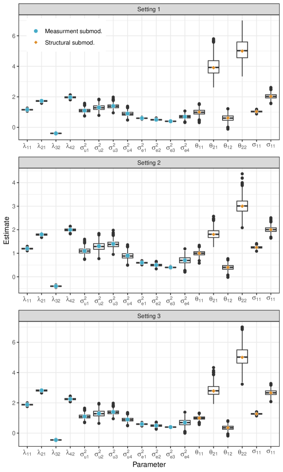
Figure 2: Final parameter estimates from the block coordinate descent algorithm for the three different settings in which the true OU process differs. Point estimates are summarized across the 1000 simulated datasets with box plots and the dots indicate the true (target) parameter values.

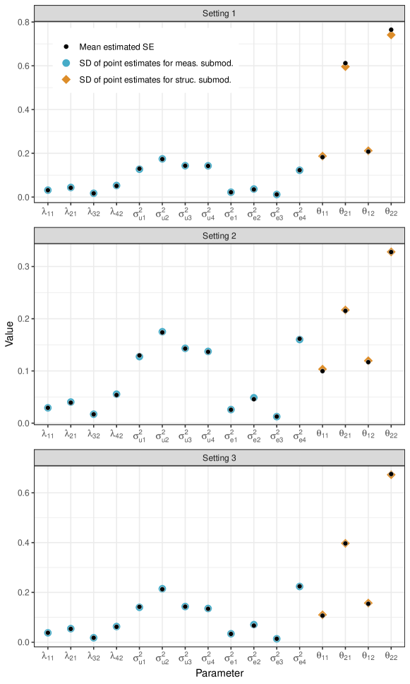
Figure 3: Comparison of estimated standard errors (from Fisher information) and standard deviation of point estimates. The similarity of the standard error estimates and empirical standard deviation suggests that the standard errors are of appropriate size. Note that the standard error estimate for $\sigma_{\epsilon_{4}}$ is missing for one datasets in Setting 3 (see Section A.9 of the supplementary material for details).

4.3 Model selection

We next carry out a simulation study in which we evaluate the ability of Akaike information criterion (AIC) and Bayesian information criterion (BIC) to correctly select the true number of latent factors among the fitted models. Formulas for AIC and BIC are given in Section A.7 of the supplementary material. Assuming the same true measurement submodel parameters as before, we now generate data from five different factor models: a one-factor model, a two-factor model with low signal (i.e., high correlation between latent factors), a two-factor model with high signal (i.e., low correlation between latent factors), a three-factor model with low signal, and a three-factor model with high signal. Data-generating parameter values are given in the Section A.8 of the supplementary material. For 100 datasets generated from each of these true models, we fit a one-, two-, and three-factor model and compare fit indices. We do not consider a four-factor model in this simulation study because our data only contain four longitudinal outcomes and so fitting a four-factor model would no longer fall into the dimension-reduction setting in which factor models are generally used.

We present model selection results in Table 1. In both the high and low signal settings, the model with the lowest AIC and BIC most often has the same number of factors as the true model used to generate the data. For models fit to data generated from a true model with three factors, BIC incorrectly selects a model with two factors more often than AIC. This difference make sense given the increased penalty that BIC places on model complexity. For datasets of this size ($N=200$), estimation becomes more difficult as the number of factors increases and so our algorithm did not converge for a few simulated datasets (see Section A.9 of the supplementary material for details).

Table 1: For datasets generated under each true model, we summarize the percent of times that the model-selection metric chose the fitted model with the indicated number of factors. When generating data from models with 2 and 3 factors, we considered two different settings: a high signal setting in which latent factors have lower correlation and a low signal setting in which latent factors have high correlation. The settings in which the fitted model has the same number of factors as the true data-generating model are emphasized with bold orange text. These results are presented for datasets on which the algorithm either converged or reached the maximum number of iterations (200) for all three models. See Section A.9 of the supplementary material for more details.

5 Application to mHealth emotion data

For illustrative purposes, we apply our method to the data on momentary emotions collected in the mHealth study. Using the OUF model, we summarize the longitudinal responses to 18 emotion-related questions as two latent factors interpreted as positive and negative affect. Positive and negative affect are two distinct-but-correlated emotional states known to be key in understanding smoking habits (e.g., Minami et al. (2014), Langdon et al. (2016), Leventhal et al. (2013), Baker et al. (2004)). The proposed model accounts for both the rapid temporal variation in these states and their correlation over time. In these data, positive affect was measured by how strongly individuals agreed with feeling happy, joyful, enthusiastic, active, calm, determined, grateful, proud, and attentive; negative affect was measured by how strongly individuals agreed with feeling sad, scared, disgusted, angry, shameful, guilty, irritable, lonely, and nervous.

When applying the OUF model, the assumed structural zeros within the loadings matrix result in positive emotions loading onto one of the latent variables, $\bm{\eta}_{1}(t)$, and negative emotions loading onto the other, $\bm{\eta}_{2}(t)$. Point estimates and 95% confidence intervals are in Figure 4. Measures of happiness, joy, and enthusiasm are most strongly correlated with positive affect and measures of sadness and irritability are most strongly correlated with negative affect. We use the estimated parameters of the OU process to understand the latent dynamics of positive and negative affect by plotting the degree of correlation for these two latent variables across varying time intervals between consecutive observations (see Figure 5). We see that positive and negative affect are negatively correlated as expected, and that the correlation between the latent states decays slowly.

We also fit a univariate OUF model and a trivariate OUF model and compare these models to the bivariate OUF model. In the univariate OUF model, all emotions are assumed to be generated from a single common underlying factor; in the trivariate OUF model, we further divide the positive emotions into two latent factors that we call high arousal positive affect (measured by feeling grateful, proud, enthusiastic, active, determined, attentive) and no-to-low arousal positive affect (measured by feeling calm, happy, and joyful), while the negative emotions are still assumed to be generated from one latent factor. Coefficient estimates from these fitted models are given in Section B.1 of the supplementary material.

Both AIC and BIC indicate that, of the three models considered, the two factor model fits best: $AIC_{\text{1 factor}}=123,309$ vs. $AIC_{\text{2 factors}}=121,069$ vs. $AIC_{\text{3 factors}}=124,957$ and $BIC_{\text{1 factor}}=123,791$ vs. $BIC_{\text{2 factor}}=121,577$ vs. $BIC_{\text{3 factor}}=125,509$. We provide more details on the calculation of AIC and BIC in Section B.1 of the supplementary material. Psychological literature supports our conclusion that two factors represent our data better than one as it suggests that positive and negative affect are not opposites, rather they capture distinct-but-correlated components of psychological state (Reich, Zautra, and Davis, 2003). The lower AIC and BIC of the two factor model compared to the three factor model suggest that the emotions corresponding to high arousal positive affect and no-to-low arousal positive affect are not different enough to justify the additional complexity of the three factor model given the current data.

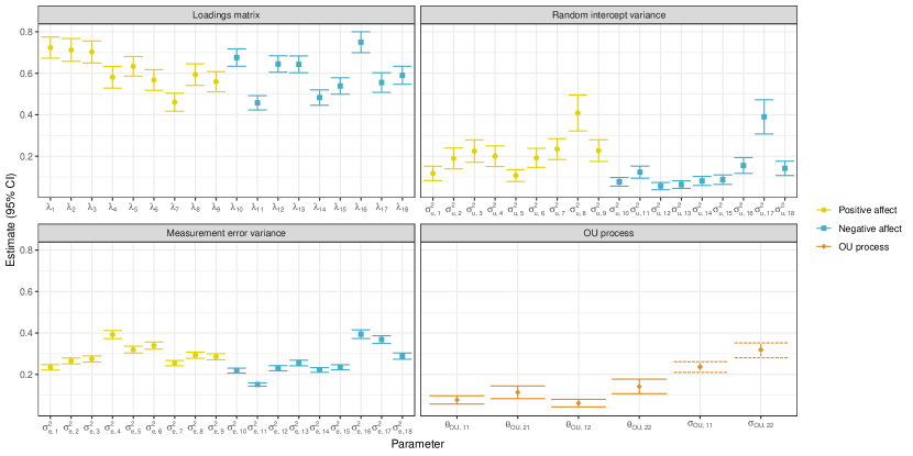
Figure 4: Point estimates and corresponding 95% confidence intervals (CI) for each of the parameter matrices in our OUF model. Intervals for OU parameters $\sigma_{11}$ and $\sigma_{22}$ are based on a parametric bootstrap. Because we assume structural zeros in the loadings matrix are known, each emotion has only a single loading. Parameter subscripts 1-18 correspond to the emotions as follows: 1 = happy, 2 = joyful, 3 = enthusiastic, 4 = active, 5 = calm, 6 = determined, 7 = grateful, 8 = proud, 9 = attentive, 10 = sad, 11 = scared, 12 = disgusted, 13 = angry, 14 = ashamed, 15 = guilty, 16 = irritable, 17 = lonely, 18 = nervous.

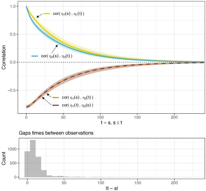
Figure 5: The top panel shows the decay in autocorrelation and cross-correlation between latent factors that represent positive affect ($\eta_{1}(t)$) and negative affect ($\eta_{2}(t)$) across increasing gap times, where time is measured in hours. Curves are calculated using OU parameters estimated from emotions measured in the mHealth study. The shaded bands indicate the 2.5th and 97.5th percentiles of a parametric bootstrap. The bottom plot summarizes the distribution of the observed gap times (in hours) between measurements for all individuals in the mHealth study.

6 Discussion

We developed a dynamic OUF model that combines a factor model to summarize multivariate observed longitudinal outcomes as lower dimensional latent factors and an OU process to describe the temporal evolution of the latent factors in continuous time. By using the OU process, instead of a discrete time approach such as a VAR process, our model can be applied to irregularly-measured ILD commonly produced by mHealth studies. The OU process captures rapid variations in the correlated latent factors over time, in contrast to a multivariate mixed model that is more suitable for capturing smooth trends over time. To fit our model, we use a block coordinate descent algorithm to directly maximize the log-likelihood of the observed multivariate longitudinal outcome. We derive both the close-form likelihood of the measured outcome and the sparse precision matrix for the multivariate OU process. Our block coordinate descent algorithm leverages analytic gradients for a subset of parameters to improve computational efficiency. Finally, we applied our method to study the dynamics of emotions among smokers attempting to quit.

Through the marginal distribution of the multivariate OU process, we parameterize our likelihood in terms of the standard OU drift ($\bm{\theta}$) and volatility ($\bm{\sigma}$) parameters. Having estimates for these parameters enables us to understand the dynamics of the latent factors, including generating new trajectories using the estimated values and examining the decay in the trajectories’ correlation over time. Through examination of decay in correlation over time, our method could help inform the design of future studies that aim to collect ILD by providing insight into how frequently the longitudinal outcomes must be measured in order to capture the correlation between them.

In our simulation study in Section 4, we generated data under true OU processes that showed reasonably slow decay in correlation over time given the intervals between measurements. We found that estimation of the OU parameters is difficult if correlation decays quickly relative to gaps between measurements. When longitudinal outcomes are measured frequently enough that correlation between consecutive measurements is captured, our method consistently returns unbiased estimates of the OU process parameters. If this method were applied to data in which longitudinal outcomes are not measured often enough to capture the correlation, estimation would be difficult. Like all statistical methods, when enough signal exists in the data, our method works well. It does, however, require studies to be designed such that longitudinal outcomes are measured with sufficient frequency that the correlation between consecutive measurements is captured.

Although we use the sparse OU precision matrix, leverage the availability of analytic gradients for the measurement submodel parameters, and implement a portion of our algorithm in C++, the computation time of our estimation algorithm increases rapidly as the number of longitudinal outcomes increases. We successfully fit our model to a dataset containing 18 longitudinal outcomes but this does require approximately 27 hours. In order to make application of our model to datasets with larger numbers of longitudinal outcomes feasible, computational efficiency must be increased. However, our proposed marginal likelihood-based method has substantial computational benefits when compared to alternative methods. In comparison to the Bayesian approach proposed for fitting a similar model in Tran et al. (2021b), our approach requires less computation time. In a simulation study with $K=4$ longitudinal outcomes measured at 10-20 occasions on $N=200$ individuals, we found that estimation via our block coordinate descent algorithm required approximately 5% of the time required by the Bayesian approach proposed in Tran et al. (2021b) given the same computing resources. More details on this comparison are given in Section C.2 of the supplementary material.

Finally, the mHealth dataset to which we applied our method also contains information on demographic characteristics and on the timing of cigarette use. Including baseline covariates in either the measurement or structural submodel would be a useful extension. In behavioral science, specific emotional states, such as negative affect or craving, are expected to be correlated with cigarette use and so future work could involve combining our OUF model with a submodel for event-time outcomes. Our model could also be modified to account for treatment or for drift in the OU process to better capture the dynamics of the latent processes after a key event such as smoking cessation or relapse.

Supporting Information

Supplementary material is available with this paper. Example code and simulated data are available on Github at https://github.com/madelineabbott/OUF.

References

- Aguilar and West (2000) Aguilar, O. and West, M. (2000). Bayesian dynamic factor models and portfolio allocation. Journal of Business & Economic Statistics 18, 338–357.
- Baker et al. (2004) Baker, T. B., Piper, M., McCarthy, D. E., Majeskie, M. R., and Fiore, M. C. (2004). Addiction motivation reformulated: an affective processing model of negative reinforcement. Psychological Review 111, 33–51.
- Carvalho et al. (2008) Carvalho, C. M., Chang, J., Lucas, J. E., Nevins, J. R., Wang, Q., and West, M. (2008). High-dimensional sparse factor modeling: Applications in gene expression genomics. Journal of the American Statistical Association 103, 1438–1456.
- Cui and Dunson (2014) Cui, K. and Dunson, D. B. (2014). Generalized dynamic factor models for mixed-measurement time series. Journal of Computational and Graphical Statistics 23, 169–191.
- Dunson (2003) Dunson, D. B. (2003). Dynamic latent trait models for multidimensional longitudinal data. Journal of the American Statistical Association 98, 555–563.
- Langdon et al. (2016) Langdon, K. J., Farris, S. G., Øverup, C. S., and Zvolensky, M. J. (2016). Associations between anxiety sensitivity, negative affect, and smoking during a self-guided smoking cessation attempt. Nicotine & Tobacco Research 18, 1188–1195.
- Leventhal et al. (2013) Leventhal, A. M., Greenberg, J. B., Trujillo, M. A., Ameringer, K. J., Lisha, N. E., Pang, R. D., and Monterosso, J. (2013). Positive and negative affect as predictors of urge to smoke: Temporal factors and mediational pathways. Psychology of Addictive Behaviors: Journal of the Society of Psychologists in Addictive Behaviors 27, 262–267.
- Liu et al. (2019) Liu, M., Sun, J., Herazo-Maya, J. D., Kaminski, N., and Zhao, H. (2019). Joint models for time-to-event data and longitudinal biomarkers of high dimension. Statistics in Biosciences 11, 614–629.
- Minami et al. (2014) Minami, H., Yeh, V. M., Bold, K. W., Chapman, G. B., and McCarthy, D. E. (2014). Relations among affect, abstinence motivation and confidence, and daily smoking lapse risk. Psychology of Addictive Behaviors 28, 376–388.
- Oravecz et al. (2009) Oravecz, Z., Tuerlinckx, F., and Vandekerckhove, J. (2009). A hierarchical Ornstein-Uhlenbeck model for continuous repeated measurement data. Psychometrika 74, 395–418.
- Oravecz et al. (2016) Oravecz, Z., Tuerlinckx, F., and Vandekerckhove, J. (2016). Bayesian data analysis with the bivariate hierarchical Ornstein-Uhlenbeck process model. Multivariate Behavioral Research 51, 106–119.
- Potter et al. (2023) Potter, L. N., Yap, J., Dempsey, W., Wetter, D. W., and Nahum-Shani, I. (2023). Integrating intensive longitudinal data (ILD) to inform the development of dynamic theories of behavior change and intervention design: a case study of scientific and practical considerations. Prevention Science pages 1–13.
- Proust et al. (2006) Proust, C., Jacqmin-Gadda, H., Taylor, J. M. G., Ganiayre, J., and Commenges, D. (2006). A nonlinear model with latent process for cognitive evolution using multivariate longitudinal data. Biometrics 62, 1014–1024.
- Proust-Lima et al. (2013) Proust-Lima, C., Amieva, H., and Jacqmin-Gadda, H. (2013). Analysis of multivariate mixed longitudinal data: A flexible latent process approach. British Journal of Mathematical and Statistical Psychology 66, 470–487.
- R Core Team (2022) R Core Team (2022). R: A Language and Environment for Statistical Computing. R Foundation for Statistical Computing, Vienna, Austria.
- Reich et al. (2003) Reich, J. W., Zautra, A. J., and Davis, M. (2003). Dimensions of affect relationships: models and their integrative implications. Review of General Psychology 7, 66–83.
- Roy and Lin (2000) Roy, J. and Lin, X. (2000). Latent variable models for longitudinal data with multiple continuous outcomes. Biometrics 56, 1047–1054.
- Sy et al. (1997) Sy, J. P., Taylor, J. M. G., and Cumberland, W. G. (1997). A stochastic model for the analysis of bivariate longitudinal AIDS data. Biometrics 53, 542–555.
- Taylor et al. (1994) Taylor, J. M. G., Cumberland, W. G., and Sy, J. P. (1994). A stochastic model for analysis of longitudinal AIDS data. Journal of the American Statistical Association 89, 727–736.
- Tran et al. (2019) Tran, T. D., Lesaffre, E., Verbeke, G., and Duyck, J. (2019). Modeling local dependence in latent vector autoregressive models. Biostatistics pages 148–163.
- Tran et al. (2021b) Tran, T. D., Lesaffre, E., Verbeke, G., and Duyck, J. (2021b). Latent Ornstein-Uhlenbeck models for Bayesian analysis of multivariate longitudinal categorical responses. Biometrics 77, 689–701.
- Tran et al. (2021a) Tran, T. D., Lesaffre, E., Verbeke, G., and Molenberghs, G. (2021a). Serial correlation structures in latent linear mixed models for analysis of multivariate longitudinal ordinal responses. Statistics in Medicine 40, 578–592.
- Vatiwutipong and Phewchean (2019) Vatiwutipong, P. and Phewchean, N. (2019). Alternative way to derive the distribution of the multivariate Ornstein–Uhlenbeck process. Advances in Difference Equations 276,.
- Wang et al. (2013) Wang, X., Berger, J. O., and Burdick, D. S. (2013). Bayesian analysis of dynamic item response models in educational testing. The Annals of Applied Statistics 7, 126––153.
- Watson et al. (1988) Watson, D., Clark, L. A., and Tellegen, A. (1988). Development and validation of brief measures of positive and negative affect: The panas scales. Journal of Personality and Social Psychology 54, 1063–1070.