CoRe Optimizer: An All-in-One Solution for Machine Learning

Abstract

The optimization algorithm and its hyperparameters can significantly affect the training speed and resulting model accuracy in machine learning applications. The wish list for an ideal optimizer includes fast and smooth convergence to low error, low computational demand, and general applicability. Our recently introduced continual resilient (CoRe) optimizer has shown superior performance compared to other state-of-the-art first-order gradient-based optimizers for training lifelong machine learning potentials. In this work we provide an extensive performance comparison of the CoRe optimizer and nine other optimization algorithms including the Adam optimizer and resilient backpropagation (RPROP) for diverse machine learning tasks. We analyze the influence of different hyperparameters and provide generally applicable values. The CoRe optimizer yields best or competitive performance in every investigated application, while only one hyperparameter needs to be changed depending on mini-batch or batch learning.

1 Introduction

The optimization algorithm can crucially determine the training speed and final performance of machine learning (ML) models [1, 2]. Training of an ML model implies that a loss function needs to be minimized. The loss function is usually a sum over training data points. Instead of calculating it simultaneously for the full training data set (deterministic or batch learning), a (semi-)randomly chosen subset of the training data is often employed (stochastic or mini-batch learning). This approach can accelerate the convergence with respect to the total computation time because the loss-function accuracy increase is sub-linear for larger batch sizes. To update the weights of the ML model, first-order gradient-based iterative optimization schemes are dominating the field, since the memory demand and computation time per step of second-order optimizers is often too high. In general, the optimization aims at a loss function’s local minimum as a function of the model’s weights because it is sufficient for most ML applications to find weight values with low loss rather than the global minimum.

The simplest form of stochastic first-order minimization for high-dimensional parameter spaces is stochastic gradient decent (SGD) [3]. In SGD, the negative gradient of the loss function with respect to each weight is multiplied by a constant learning rate and the product is subtracted from the respective weight in each update. The loss function gradient is adapted in stochastic gradient decent with momentum (Momentum) [4] and Nesterov accelerated gradient (NAG) [5, 6]. These methods aim to improve convergence by a momentum in the weight updates, as the gradients are based on stochastic estimates. In a different fashion, adaptive gradient (AdaGrad) [7], adaptive delta (AdaDelta) [8], and root mean square propagation (RMSprop) [9] apply the ordinary loss function gradient combined with a weight-specific, adapted learning rate. Adaptive moment estimation (Adam) [10], adaptive moment estimation with infinity norm (AdaMax) [10], and our recently developed continual resilient (CoRe) optimizer [11] combine momentum with individually adapted learning rates. In resilient backpropagation (RPROP) [12, 13] only the sign of the loss function gradient is employed with individually adapted learning rates.

Apart from these optimizers, which are applied in this work, many more optimizers have been developed for ML applications in recent years. For example, the modification of the first moment estimation of Adam yields Nesterov-accelerated adaptive moment estimation (NAdam) [14] and the modification of the second moment AMSGrad [15]. Nesterov momentum is also employed in adaptive Nesterov momentum (Adan) [16]. Moreover, AdaFactor [17], AdaBound [18], AdaBelief [19], AdamW [20], PAdam [21], RAdam [22], AdamP [23], Lamb [24], Gravity [25], and Lion [26] are further examples of the large zoo of optimizers. They often represent incremental improvements of parent algorithms. We note that these optimizers can be used in applications beyond ML as well. Furthermore, second-order optimizers have been proposed such as adaptive estimates of the Hessian (AdaHessian) [27] and second-order clipped stochastic optimization (Sophia) [28]. To acquire an overview of the performance differences among these optimizers, extensive benchmarks are required [29, 30, 31]. Statistical averaging and uncertainty quantification are indispensable in these benchmarks for validation.

To ease the burden on an ML practitioner in the optimizer choice, an optimizer is desired which performs well on diverse ML tasks. Moreover, a generally applicable set of optimizer hyperparameters is required which works out-of-the-box avoiding time consuming hyperparameter tuning. At most, a single intuitive hyperparameter may require to be adapted coarsely, while its value needs to be easy to estimate. Furthermore, the ideal optimizer features fast and smooth convergence to high accuracy with low computational burden.

The Adam optimizer is not an obviously superior, but viable choice for many ML tasks [31]. Therefore, Adam became the most frequently applied optimizer with adaptive learning rates. Since our CoRe optimizer has outperformed Adam on the task of training a lifelong machine learning potential (lMLP) [11], it is obvious to assess its performance on diverse ML tasks and compare the outcome with that of various aforementioned optimizers. Such a broad performance evaluation further allows us to obtain generally valid hyperparameters for the CoRe optimizer to obtain an all-in-one solution.

As a benchmark, we examine a set of fast running ML tasks provided in PyTorch [32]. First, for the MNIST handwritten digits [33] and Fashion-MNIST [34] data sets we run mini-batch learning to do variational auto-encoding (AED and ADF) [35] and image classification (ICD and ICF). The latter is done by convolutional neural networks [36] with rectified linear units (ReLU) [37], dropout [38], max pooling [39], and softmax. Second, for the cart-pole problem [40] we perform naive reinforcement learning (NR) with a feed-forward linear neural network [41], dropout, ReLU, and softmax and reinforcement learning by an actor-critic algorithm (RA) [42]. Third, for the BSD300 data set [43] we carry out single image super-resolution (SR) with upscale factor four by sub-pixel convolutional neural networks [44] employing relatively large mini-batches. Fourth, we run batch learning of the Cora data set [45] for semi-supervised classification (SS) with graph convolutional networks [46] and dropout as well as of a sine wave for time sequence prediction (TS) with a long short-term memory (LSTM) cell [47].

In addition, we evaluate the optimizers in training of a machine learning potential [48, 49, 50, 51, 52, 53], which is a representation of the potential energy surface of a chemical system. It can be employed in atomistic simulations to calculate chemical properties and reactivity. One method example among many others is a high-dimensional neural network potential [54, 55] which takes as input the chemical element types and atomic coordinates and in required cases atomic charges and spins [56, 57, 58] to calculate the energy and atomic forces of systems ranging from organic molecules over liquids to inorganic materials including multi-component systems such as interfaces [59, 60, 61, 11]. In this work, we repeat the stationary learning of an lMLP based on an ensemble of ten high-dimensional neural network potentials, which employ element-embracing atom-centered symmetry functions as descriptors [11]. The lMLP is trained on 8600 S${}_{\text{N}}$2 reaction systems with lifelong adaptive data selection.

This work is organized as follows: In Section 2, we summarize the applied optimization algorithms, and in Section 3, we compile the computational details. In Section 4, we analyze the resulting training speed and final accuracy for the PyTorch ML task examples and lMLPs. This work ends with a conclusion in Section 5.

2 Methods

2.1 Continual Resilient (CoRe) Optimizer

The CoRe optimizer [11] is a first-order gradient-based optimizer for stochastic and deterministic iterative optimizations. It adapts the learning rates individually for each weight $w_{\xi}$ depending on the optimization progress. These learning rate adjustments are inspired by the Adam optimizer [10], RPROP [12, 13], and the synaptic intelligence method [62].

Exponential moving averages of the loss function gradient and its square,

$$g_{\xi}^{\tau} =\beta_{1}^{\tau}\cdot g_{\xi}^{\tau-1}+\left(1-\beta_{1}^{\tau}\right)\frac{\partial L^{t}}{\partial w_{\xi}^{t}}\ ,$$ (1)

$$h_{\xi}^{\tau} =\beta_{2}\cdot h_{\xi}^{\tau-1}+\left(1-\beta_{2}\right)\left(\frac{\partial L^{t}}{\partial w_{\xi}^{t}}\right)^{2}\ ,$$ (2)

with decay rates $\beta_{1}^{\tau},\beta_{2}\in[0,1)$, are employed in minimization in analogy to the Adam optimizer. For maximization, the sign of the loss function gradient in Equation (1) has to be inverted. In the CoRe optimizer, $\beta_{1}$ is a function of the individual weight update counter $\tau$,

$$\beta_{1}^{\tau}=\beta_{1}^{\mathrm{b}}+\left(\beta_{1}^{\mathrm{a}}-\beta_{1}^{\mathrm{b}}\right)\exp\left[-\left(\frac{\tau-1}{\beta_{1}^{\mathrm{c}}}\right)^{2}\right]\ ,$$ (3)

whereby $\tau$ can vary from the counter of gradient calculations $t$ if some optimization steps do not update every weight. The initial decay $\beta_{1}^{\mathrm{a}}\in[0,1)$ is converted by a Gaussian with width $\beta_{1}^{\mathrm{c}}>0$ to the final decay $\beta_{1}^{\mathrm{b}}\in[0,1)$. The smaller $\beta_{1}^{\tau}$, the higher is the dependence on the current gradient, while a larger $\beta_{1}^{\tau}$ leads to a slower decay of previous gradient contributions.

The Adam-like adaption of the weight-specific learning rates,

$$u_{\xi}^{\tau}=\frac{g_{\xi}^{\tau}}{1-\left(\beta_{1}^{\tau}\right)^{\tau}}\left\{\left[\frac{h_{\xi}^{\tau}}{1-\left(\beta_{2}\right)^{\tau}}\right]^{\tfrac{1}{2}}+\epsilon\right\}^{-1}\ ,$$ (4)

employs the quotient of the moving averages $g_{\xi}^{\tau}$ and $(h_{\xi}^{\tau})^{\tfrac{1}{2}}$, which are corrected with respect to their initialization bias toward zero ($g_{\xi}^{0},h_{\xi}^{0}=0$). For numerical stability $\epsilon\gtrapprox 0$ is added in the denominator. This quotient is invariant to gradient rescaling and introduces a form of step size annealing. Therefore, $u_{\xi}^{\tau}$ changes from $\pm 1$ in the first optimization step $\tau=1$ toward zero in well-behaving optimizations.

The plasticity factor,

$$P_{\xi}^{\tau}=\begin{cases}0&\begin{array}[]{l}\mathrm{for}\ \tau>t_{\mathrm{hist}}\\ \land\ S_{\xi}^{\tau-1}\ \mathrm{top}\text{-}n_{\mathrm{frozen},\chi}\ \mathrm{in}\ \mathbf{S}_{\chi}^{\tau-1}\end{array}\\ 1&\begin{array}[]{l}\mathrm{otherwise}\end{array}\end{cases}\ ,$$ (5)

aims to improve the stability-plasticity balance by regularization in the weight updates. Therefore, weight groups $\chi$ are specified—for example, a layer in a neural network—and the weight-specific importance scores $\mathbf{S}_{\chi}^{\tau-1}$ (see Equation (8) below) are compared within these groups. When $\tau>t_{\mathrm{hist}}>0$, $P_{\xi}^{\tau}$ can freeze the weights with the $n_{\mathrm{frozen},\chi}\geq 0$ highest importance scores in their group in update $\tau$ to mitigate forgetting of previous knowledge.

The RPROP-like learning rate adaption,

$$s_{\xi}^{\tau}=\begin{cases}\mathrm{min}\left(\eta_{+}\cdot s_{\xi}^{\tau-1},s_{\mathrm{max}}\right)&\mathrm{for}\ g_{\xi}^{\tau-1}\cdot g_{\xi}^{\tau}\cdot P_{\xi}^{\tau}>0\\ \mathrm{max}\left(\eta_{-}\cdot s_{\xi}^{\tau-1},s_{\mathrm{min}}\right)&\mathrm{for}\ g_{\xi}^{\tau-1}\cdot g_{\xi}^{\tau}\cdot P_{\xi}^{\tau}<0\\ s_{\xi}^{\tau-1}&\mathrm{for}\ g_{\xi}^{\tau-1}\cdot g_{\xi}^{\tau}\cdot P_{\xi}^{\tau}=0\end{cases}\ ,$$ (6)

depends only on the sign of the gradient moving average $g_{\xi}^{\tau}$ and not on its magnitude leading to a robust optimization. Sign inversions from $g_{\xi}^{\tau-1}$ to $g_{\xi}^{\tau}$ often signalize a jump over a minimum in the previous update. Hence, the step size $s_{\xi}^{\tau-1}$ is reduced by the decrease factor $\eta_{-}\in(0,1]$ in this case, while it is enlarged by the increase factor $\eta_{+}\geq 1$ for constant signs to speed up convergence. The updated step size $s_{\xi}^{\tau}$ is bounded by the minimal and maximal step sizes $s_{\mathrm{min}},s_{\mathrm{max}}>0$. For $g_{\xi}^{\tau-1}\cdot g_{\xi}^{\tau}\cdot P_{\xi}^{\tau}=0$, the step size update is omitted. The initial step size $s_{\xi}^{0}=s_{\xi}^{1}$ is a hyperparameter of the optimization.

The weight decay,

$$w_{\xi}^{t}=\left(1-d_{\chi}\cdot\left|u_{\xi}^{\tau}\right|\cdot P_{\xi}^{\tau}\cdot s_{\xi}^{\tau}\right)w_{\xi}^{t-1}-u_{\xi}^{\tau}\cdot P_{\xi}^{\tau}\cdot s_{\xi}^{\tau}\ ,$$ (7)

with group-specific hyperparameter $d_{\chi}\in[0,(s_{\mathrm{max}})^{-1})$, targets to reduce the overfitting risk by prevention of strong weight in- or decreases. It is proportional to the product of $d_{\chi}$ and the absolute weight update $|u_{\xi}^{\tau}|\cdot P_{\xi}^{\tau}\cdot s_{\xi}^{\tau}$, i.e., the more stable the weight value the less it is affected by the weight decay. Subsequently, the signed weight update $u_{\xi}^{\tau}\cdot P_{\xi}^{\tau}\cdot s_{\xi}^{\tau}$ is subtracted to obtain the updated weight $w_{\xi}^{t}$. The weight values are therefore bound between $-(d_{\chi})^{-1}$ and $(d_{\chi})^{-1}$ in well-behaving optimizations, i.e., $u_{\xi}^{\tau}\leq\pm 1$.

The importance score value,

$$S_{\xi}^{\tau}=\begin{cases}\begin{array}[]{l}S_{\xi}^{\tau-1}+\left(t_{\mathrm{hist}}\right)^{-1}g_{\xi}^{\tau}\cdot u_{\xi}^{\tau}\cdot P_{\xi}^{\tau}\cdot s_{\xi}^{\tau}\end{array}&\mathrm{for}\ \tau\leq t_{\mathrm{hist}}\vspace{0.075cm}\\ \begin{array}[]{l}\left[1-\left(t_{\mathrm{hist}}\right)^{-1}\right]S_{\xi}^{\tau-1}\\ +\left(t_{\mathrm{hist}}\right)^{-1}g_{\xi}^{\tau}\cdot u_{\xi}^{\tau}\cdot P_{\xi}^{\tau}\cdot s_{\xi}^{\tau}\end{array}&\mathrm{otherwise}\end{cases}\ ,$$ (8)

ranks the weight importance by taking into account weight-specific contributions to previously estimated loss function decreases. This ansatz is inspired by the synaptic intelligence method. The importance scores enable to identify the most important weights in previous updates, which can be frozen by the plasticity factors (Equation (5)) in following updates to improve the stability-plasticity balance. The product of gradient moving average and signed weight update is employed to estimate the loss function decrease. Since the weight update sign is not inverted, the higher positive the importance score, the larger is the loss function decrease. Starting with $S_{\xi}^{0}=0$, the mean of $g_{\xi}^{\tau}\cdot u_{\xi}^{\tau}\cdot P_{\xi}^{\tau}\cdot s_{\xi}^{\tau}$ over $\tau\leq t_{\mathrm{hist}}$ is calculated. For $\tau>t_{\mathrm{hist}}$, the importance score is determined as exponential moving average with decay $1-(t_{\mathrm{hist}})^{-1}$.

2.2 SGD

SGD [3] subtracts the product of a constant learning rate $\gamma$ and the loss function gradient from the weights $w_{\xi}^{t-1}$ in the weight updates,

$$w_{\xi}^{t}=w_{\xi}^{t-1}-\gamma G_{\xi}^{\tau}\ ,$$ (9)

with

$$G_{\xi}^{\tau}=\frac{\partial L^{t}}{\partial w_{\xi}^{t}}\ .$$ (10)

2.3 Momentum

An additional momentum (Momentum) [4] can be introduced in SGD by replacing $G_{\xi}^{\tau}$ in Equation (9) by

$$m_{\xi}^{\tau}=\mu\cdot m_{\xi}^{\tau-1}+G_{\xi}^{\tau}\ ,$$ (11)

with the momentum factor $\mu$ and $m_{\xi}^{1}=G_{\xi}^{1}$ [32].

2.4 NAG

NAG [5, 6] is SGD with Nesterov momentum, i.e, $G_{\xi}^{\tau}$ in Equation (9) is substituted by

$$n_{\xi}^{\tau}=\mu\cdot m_{\xi}^{\tau}+G_{\xi}^{\tau}\ .$$ (12)

2.5 Adam

The algorithm of the Adam optimizer [10] is given by Equations (1) (with constant $\beta_{1}$), (2), (4), and (9), whereby $G_{\xi}^{\tau}$ in Equation (9) is replaced by $u_{\xi}^{\tau}$. In comparison to the CoRe optimizer, Adam misses the $\tau$ dependence of the decay rate $\beta_{1}$, the plasticity factors $P_{\xi}^{\tau}$, the RPROP-like learning rate adaption $s_{\xi}^{\tau}$, and the weight decay. The latter can be introduced in Adam as well as in many other optimizers also by adding $d\cdot w_{\xi}^{t-1}$ to the loss function gradient as second operation of an optimization iteration after the possible sign inversion for maximization. A further alternative is to subtract instead $d\cdot\gamma\cdot w_{\xi}^{t-1}$ from $w_{\xi}^{t-1}$ as in AdamW [20].

2.6 AdaMax

The difference of the AdaMax optimizer [10] compared to Adam is that the term in curly brackets in Equation (4) is replaced by the infinity norm,

$$k_{\xi}^{\tau}=\mathrm{max}\left(\beta_{2}\cdot k_{\xi}^{\tau-1},\left|G_{\xi}^{\tau}+\epsilon\right|\right)\ ,$$ (13)

with $k_{\xi}^{0}=0$.

2.7 RMSprop

In RMSprop [9] the loss function gradient is divided by the moving average of its magnitude,

$$w_{\xi}^{t}=w_{\xi}^{t-1}-\gamma G_{\xi}^{\tau}\left[\left(h_{\xi}^{\tau}\right)^{\tfrac{1}{2}}+\epsilon\right]^{-1}\ .$$ (14)

Hence, the difference to the Adam optimizer is that the loss function gradient $G_{\xi}^{\tau}$ is applied instead of the gradient moving average $g_{\xi}^{\tau}$ and the initialization bias correction is omitted.

2.8 AdaGrad

The AdaGrad optimizer [7] differs from RMSprop by the replacement of $h_{\xi}^{\tau}$ in Equation (14) by

$$b_{\xi}^{\tau}=b_{\xi}^{\tau-1}+\left(G_{\xi}^{\tau}\right)^{2}\ ,$$ (15)

with $b_{\xi}^{0}=0$.

2.9 AdaDelta

The adaptive learning rate in the AdaDelta optimizer [8] is established by

$$w_{\xi}^{t}=w_{\xi}^{t-1}-\gamma G_{\xi}^{\tau}\left(\frac{l_{\xi}^{\tau-1}+\epsilon}{h_{\xi}^{\tau}+\epsilon}\right)^{\tfrac{1}{2}}\ ,$$ (16)

with

$$l_{\xi}^{\tau}=\beta_{2}\cdot l_{\xi}^{\tau-1}+\left(1-\beta_{2}\right)\frac{l_{\xi}^{\tau-1}+\epsilon}{h_{\xi}^{\tau}+\epsilon}\left(G_{\xi}^{\tau}\right)^{2}$$ (17)

and $l_{\xi}^{0}=0$. Hence, in comparison to the RMSprop algorithm the factor $\left(l_{\xi}^{\tau-1}+\epsilon\right)^{\tfrac{1}{2}}$ is applied additionally in the weight update and the order of adding $\epsilon$ to $h_{\xi}^{\tau}$ and taking the square root is inverted.

2.10 RPROP

RPROP [12, 13] is based on Equation (6), whereby $G_{\xi}^{\tau-1}\cdot G_{\xi}^{\tau}$ is employed instead of $g_{\xi}^{\tau-1}\cdot g_{\xi}^{\tau}\cdot P_{\xi}^{\tau}$. In addition, a backtracking weight step is applied by setting $G_{\xi}^{\tau}=0$ when $G_{\xi}^{\tau-1}\cdot G_{\xi}^{\tau}<0$. The weight update is given by

$$w_{\xi}^{t}=w_{\xi}^{t-1}-s_{\xi}^{\tau}\cdot\mathrm{sgn}\left(G_{\xi}^{\tau}\right)\ .$$ (18)

3 Computational Details

The PyTorch ML task examples [63] were solely modified to embed them in the extensive benchmark without touching the ML models and trainings. The only exception was the removal of the learning rate scheduler in ICD and ICF to assess exclusively the performance of the optimizer. The batch sizes of the ML tasks AED, AEF, ICD, and ICF were 64 of in total 60000 training data points and the batch size of SR was 10 of 200. More than $10^{4}$ training episodes in NR and RA were considered as failed and were accounted as an error of infinity. The employed scripts with all details on the models, trainings, and error definitions are available on Zenodo [64] alongside the compiled raw results as well as plot and analysis scripts. Moreover, the repository contains the updated CoRe optimizer software, which is compatible to use with PyTorch. Moreover, the lMLP software [65] was extended to integrate all optimizers and is also available in this Zenodo repository [64] alongside lMLP results as well as model and training details. The latter were taken over from Reference [11]. The lMLP training employed lifelong adaptive data selection and a fit fraction per epoch of $10\%$ of all 7740 training structures.

Each ML task was performed for each optimizer setting with 20 different sets of random numbers. These sets were the same for each optimizer and they ensured differently initialized weights (and different selection of training and test data). The mean test set error $E_{i}^{\mathrm{test}}$ and its standard deviation $\Delta E_{i}^{\mathrm{test}}$ of ML task $i$ were calculated for each set as a function of the training epoch $n_{\mathrm{epoch}}$ to evaluate convergence. To determine the final accuracy, for the minimal test set error in each of the 20 trainings the mean $E_{i}^{\mathrm{test,min}}$ and standard deviation $\Delta E_{i}^{\mathrm{test,min}}$ were calculated, i.e., early stopping was applied. For reinforcement learning (NR and RA) the mean number of training episodes until a reward of 475 [66] was taken to quantify $E_{i}^{\mathrm{test}}$. 8 of 20 NAG trainings for AEF failed even for the best learning rate value. These trainings were penalized with a constant error of 1000. For lMLPs the total test loss according to Equation (10) in Reference [11] determined the training epoch with minimal error. In this way, the mean squared error of the energies was weighted with a factor $q^{2}=10.9^{2}$ in the loss function, while that of the atomic force components was not scaled. We evaluated the mean error based on the errors of all 20 lMLPs in each of the 20 training epochs where an individual lMLP showed minimal error, i.e., 400 error values were included. In this way, the error was still calculated from advanced training states, while it was also sensitive to the smoothness of the training processes as early stopping is difficult to apply in practise in lifelong machine learning.

To compare the final accuracy among different optimizers for ML task $i$, the inverse of the error $E_{i}^{\mathrm{test,min}}$ relative to the result of best performing optimizer in ML task $i$ was calculated,

$$A_{i}=\dfrac{\min_{i}\left(E_{i}^{\mathrm{test,min}}\right)}{E_{i}^{\mathrm{test,min}}}\ .$$ (19)

The uncertainty interval $[A^{-},A^{+}]$ for the accuracy score was based on the test set error’s standard deviation $\Delta E_{i}^{\mathrm{test}}$,

$$A_{i}^{\pm}=\dfrac{\min_{i}\left(E_{i}^{\mathrm{test,min}}\right)}{\mathrm{max}\left(0,E_{i}^{\mathrm{test,min}}\mp\Delta E_{i}^{\mathrm{test,min}}\right)}\ .$$ (20)

For comparison of different optimizers with regard to the overall accuracy, the arithmetic mean $\overline{A}$ of the ML task accuracy scores $A_{i}$ was calculated. The uncertainty interval $[\overline{A}^{-},\overline{A}^{+}]$ was determined by the means of $A_{i}^{-}$ and $A_{i}^{+}$, respectively.

The PyTorch version 2.0.0 [32] and its default settings were applied for the optimizers AdaDelta, AdaGrad, Adam, AdaMax, Momentum, NAG, RMSprop, RPROP, and SGD (see Tables S1 and S3 in the Supporting Information for all hyperparameter values). Weight decay was by default only applied by the CoRe optimizer. The momentum factor in Momentum and NAG was $\mu=0.9$. Adam^∗ employs a different $\beta_{2}$ value of $0.99$ and RPROP^∗ a different $\eta_{-}$ value of $0.7375$. The learning rates $s_{\xi}^{0}$ of RPROP, RPROP^∗, and the CoRe optimizer were set to $10^{-3}$. For the learning rate $\gamma$ of the other optimizers and the maximal step size $s_{\mathrm{max}}$ of RPROP, RPROP^∗, and the CoRe optimizer, the values $0.0001$, $0.001$, $0.01$, $0.1$, and $1$ were tested for each PyTorch ML task example. The value yielding the lowest $\Delta E_{i}^{\mathrm{test,min}}$ was employed in the performance evaluation (see Table S2 in the Supporting Information). For lMLP training the two most likely options according to the PyTorch ML task results were tested (see Table S4 in the Supporting Information).

4 Results and Discussion

4.1 General Recommendations for CoRe Optimizer Hyperparameter Values

A generally applicable set of CoRe optimizer hyperparameter values has been obtained from a benchmark on nine ML tasks including seven different models and six different data sets. The training processes span the entire range from learning on small mini-batches to full data set batch learning. Based on this benchmark we generally recommend the hyperparameter values $\beta_{1}^{\mathrm{a}}=0.7375$, $\beta_{1}^{\mathrm{b}}=0.8125$, $\beta_{1}^{\mathrm{c}}=250$, $\beta_{2}=0.99$, $\epsilon=10^{-8}$, $\eta_{-}=0.7375$, $\eta_{+}=1.2$, $s_{\mathrm{min}}=10^{-6}$, $s_{\xi}^{0}=10^{-3}$, $d_{\chi}=0.1$, and $t_{\mathrm{hist}}=250$. The number of frozen weights per group $n_{\mathrm{frozen,\chi}}$ can often be specified as a fraction of frozen weights per group $p_{\mathrm{frozen,\chi}}$. Well working values of $p_{\mathrm{frozen,\chi}}$ are typically in the interval between $0$ (without stability-plasticity balance) and about $10\%$. The maximum step size $s_{\mathrm{max}}$ is recommended to be $10^{-3}$ for mini-batch learning, $1$ for batch learning, and $10^{-2}$ for intermediate cases. $s_{\mathrm{max}}$ is the main hyperparameter like the learning rate $\gamma$ in many other optimizers.

4.2 Optimizer Performance Evaluation for Diverse Machine Learning Tasks

To assess the performance of the CoRe optimizer in comparison to nine other optimizers with in total eleven different hyperparameter settings, relative accuracy scores for nine ML tasks were calculated for these optimizers (Figure 1). For mini-batch learning on small batch sizes ($0.1\%$ for AED, AEF, ICD, and ICF) the popular Adam optimizer and our CoRe optimizer perform best, while especially RPROP yields poor accuracy because it cannot handle well stochastic gradient fluctuations. RPROP is intended for batch learning which becomes obvious by the very high accuracy scores for SS and TS. For these ML tasks, RPROP and the CoRe optimizer achieve the highest accuracy scores. In the intermediate case, i.e., mini-batch learning with rather large batch sizes ($5\%$ for SR and $10\%$ for lMLP training (Figure 4)), both Adam and RPROP perform well with Adam having a small advantage over RPROP. However, the CoRe optimizer outperforms both in this case. In total, the CoRe optimizer achieves the highest final accuracy in four tasks and lMLP training, Adam in two tasks, and RPROP in one task. Therefore, the CoRe optimizer is well-rounded and obviously achieves the highest overall accuracy score (Figure 2), while that of Adam is second highest.

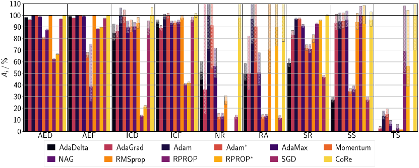
Figure 1: Final accuracy scores $A_{i}$ and their uncertainties of various ML tasks $i$ trained by different optimizers.

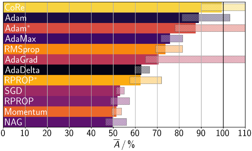
Figure 2: Final accuracy score $\overline{A}$ and its uncertainty averaged over the ML tasks shown in Figure 1 for different optimizers.

Moreover, the learning speed of the CoRe optimizer in reinforcement learning (NR and RA) is also better than for the other optimizers (Figure 1), while RPROP is not able to learn the task in the maximal number of episodes in every training. While Adam reaches the highest score for NR and the CoRe optimizer for RA, the lower bound of the uncertainty interval is highest for the CoRe optimizer in both NR and RA. The CoRe optimizer’s convergence speed of the mean test set errors for the other ML tasks is similar to Adam for mini-batch learning and similar to RPROP for batch learning (see Figures S1 to S7 and S9 in the Supporting Information).

In general, for the chosen set of ML tasks the optimizers which combine momentum and individually adapted learning rates (CoRe, Adam, and AdaMax) perform better than those which only apply individually adapted learning rates (RMSprop, AdaGrad, and AdaDelta) (Figure 2). However, there are relatively large differences among the CoRe optimizer, Adam, and AdaMax, while RMSprop is only slightly worse than AdaMax. The final accuracy obtained by pure SGD is significantly worse than that of the aforementioned optimizers. However, for these nine ML tasks it is still slightly better than that of the optimizers which employ only momentum (Momentum and NAG). The overall accuracy of RPROP is in between those applying individually adapted learning rates and SGD for these ML tasks. However, the order is, of course, dependent on the fraction of mini-batch and batch learning ML tasks.

The best single model performances obtained by the CoRe optimizer are provided in Table S5 and Figures S10 (a) and (b) and S11 in the Supporting Information. For SS we can compare the final accuracy directly to the original work with $81.5\%$ correct test set classifications [46]. Due to training by the CoRe optimizer, the best graph convolutional network for SS achieves a test set classification accuracy of $84.2\%$.

4.3 Performance Dependence on Hyperparameter Values

The CoRe optimizer hyperparameters were adjusted on this set of ML tasks, while we applied general recommendations for the other optimizers which were obtained in benchmarks of other ML tasks. To probe whether the comparison is fair, we adjust also the hyperparameters of the second best performing optimizer Adam on this set of ML tasks. Similar to the CoRe optimizer, the hyperparameters $\beta_{1}=0.8125$ and $\beta_{2}=0.99$ yield high final accuracy for the ML tasks. Still, from any of the four possible combinations of $\beta_{1}=0.8125,0.9$ and $\beta_{2}=0.99,0.999$, the general Adam parametrization of $\beta_{1}=0.9$ and $\beta_{2}=0.999$ performs best. However, the accuracy difference to the second best values $\beta_{1}=0.9$ and $\beta_{2}=0.99$ is small (Adam^∗ in Figures 1 and 2). For RPROP our adjustment of $\eta_{-}$ resulted in a value of $0.7375$ analogous to the CoRe optimizer. The respective RPROP^∗ final accuracy scores are on average significantly higher than the RPROP accuracy scores (Figures 1 and 2). Hence, the adjustment of the hyperparameters can improve the general performance but the advantage of the CoRe optimizer over Adam and RPROP remains.

Another difference between the CoRe optimizer and Adam was the application of a weight decay. However, Figures S13 and S14 in the Supporting Information show that two different weight decay algorithms with each four different hyperparameters in general reduce the accuracy score for Adam. Only the weight decay as in AdamW with $d=0.001$ leads to a slightly higher overall accuracy score than obtained by Adam without weight decay. By contrast, the weight decay of the CoRe optimizer even improves the final accuracy on average (Figures S13 and S14 in the Supporting Information).

In the analysis of individual ML task performances, we note that RPROP and the CoRe optimizer show a slow convergence in the initial epochs of SS training (see Figure S6 in the Supporting Information). The reason is that large weight changes are required in the optimization and the initial step size $s_{\xi}^{0}$ is only set to $0.001$. Higher values of $s_{\xi}^{0}$ result in faster convergence to a similar final accuracy, with $s_{\xi}^{0}=0.1$ yielding a much faster convergence than obtained with Adam (see Figure S7 in the Supporting Information). However, this ML task is an extreme example with few weight updates to adjust $s_{\xi}^{\tau}$ in batch learning and the need of large weight changes. Still, as the final accuracy is the same and in most applications $s_{\xi}^{\tau}$ is fast adapted in a relatively small fraction of weight updates, the initialization of $s_{\xi}^{0}$ is in general noncritical.

Another edge case can be obtained for high maximal step size values $s_{\mathrm{max}}$ in the CoRe optimizer. While $s_{\mathrm{max}}=1$ yields a high final accuracy in TS training when early stopping is applied, the training can become unstable when continued (see Figure S8 in the Supporting Information). However, reducing $s_{\mathrm{max}}$ to $0.1$ already solves this issue (see Figure S9 in the Supporting Information).

4.4 Optimizer Performance in Training Lifelong Machine Learning Potentials

In the training of lMLPs rather large fractions of training data ($10\%$) were employed in the loss function gradient calculation. In line with the results of the PyTorch ML task examples, this kind of training best suits the CoRe optimizer followed by Adam and RPROP (Figures 3 and 4). Moreover, the general trend is confirmed that adaptive and moment based optimizers perform best, while only adaptive optimizers still yield better results than only moment based optimizers. In contrast to the PyTorch ML task examples, where the stability-plasticity balance of the CoRe optimizer with $p_{\mathrm{frozen}}$ around $0.025$ can only marginally improve the accuracy scores for AED, AEF, and SR and worsens the final accuracy for ICD and ICF (see Figure S12 in the Supporting Information), the lMLP training largely benefits from the stability-plasticity balance with $p_{\mathrm{frozen}}=0.1$.

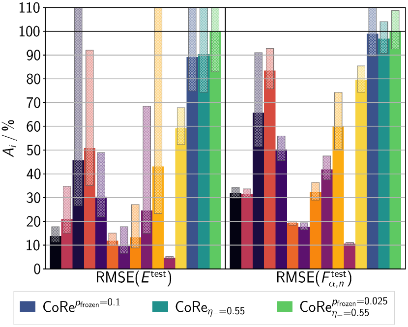
Figure 3: Final accuracy scores $A_{i}$ and their uncertainties of energy and force prediction of lMLPs trained by different optimizers.

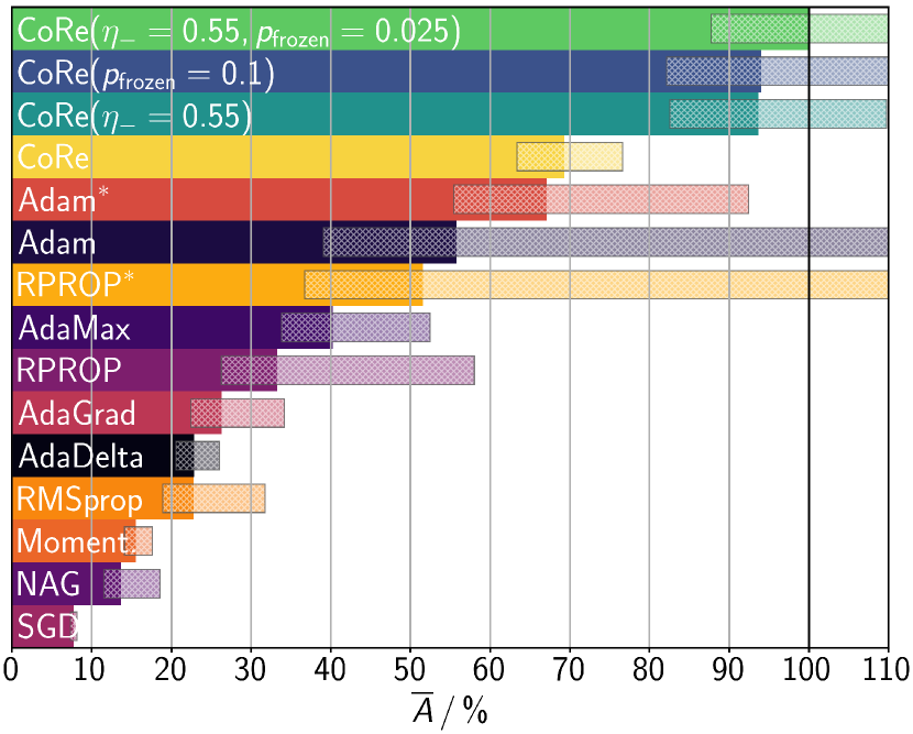
Figure 4: Final accuracy score $\overline{A}$ and its uncertainty combining energy and force prediction of lMLPs for different optimizers.

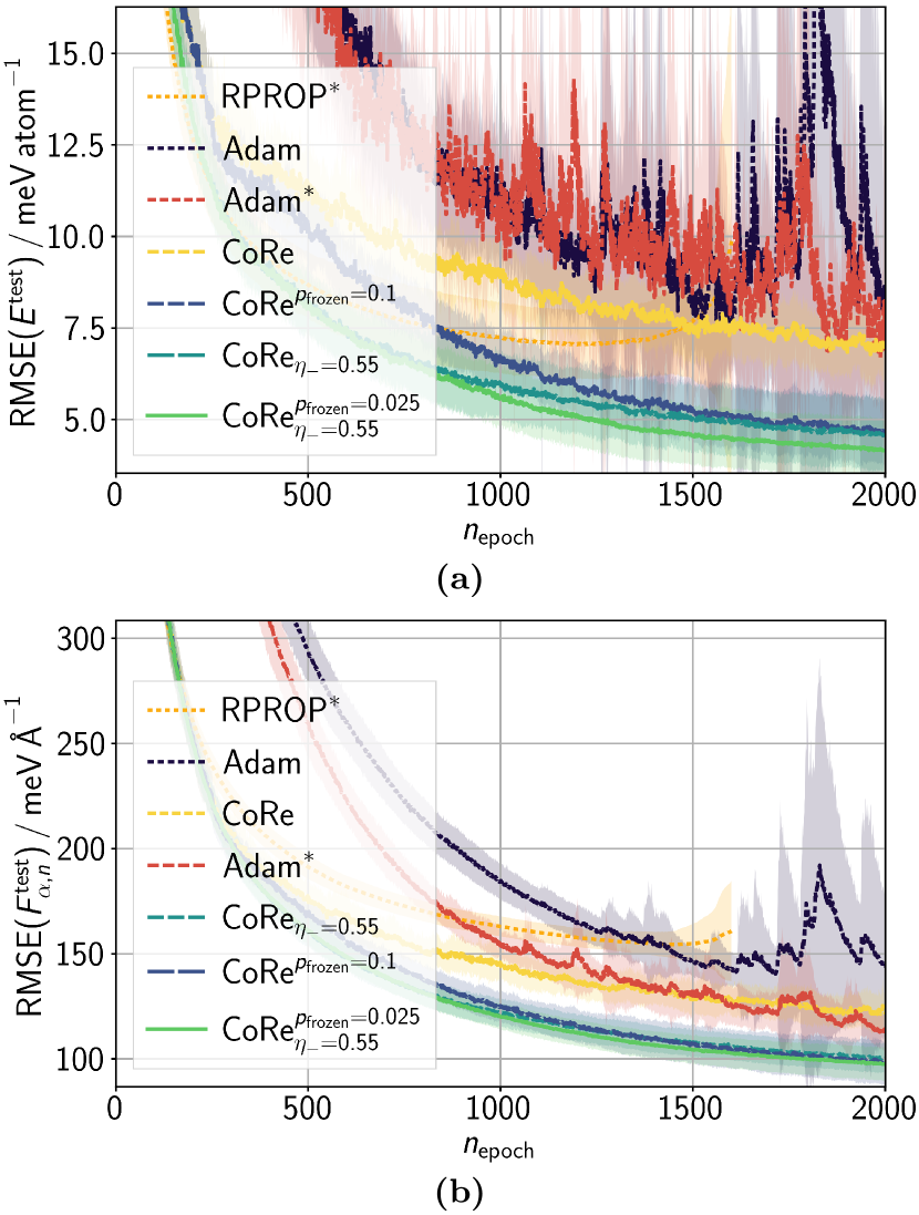
Figure 5: Test set RMSEs of (a) energy $E^{\mathrm{test}}$ and (b) atomic force components $F_{\alpha,n}^{\mathrm{test}}$ as a function of the training epoch $n_{\mathrm{epoch}}$ for the lMLP compared to the DFT reference. The results are shown for the seven optimizers yielding highest final accuracy. The less often a line is broken, the lower is the final error. Uncertainty intervals are shown in pale color of the respective line.

Moreover, the stability-plasticity balance smoothens the training convergence as shown in the test set root mean square errors (RMSEs) of energies and atomic force components as a function of the training epochs (Figures 5 (a) and (b)). The CoRe optimizer yields smoother convergence than Adam, which is beneficial, for example, in lifelong machine learning where the lMLP needs to be ready for application in every training stage. The accuracy scores in Figures 3 and 4 take into account the convergence smoothness (see Section 3) in contrast to the accuracy scores in Figures S15 and S16 in the Supporting Information which are only based on the individual lMLP early stopping results. The latter is beneficial for the Adam results but still the CoRe optimizer with stability-plasticity balance outperforms Adam. The convergence speed is also much higher for the CoRe optimizer than for Adam. This observation is in line with the convergence of the SR ML task (see Figure S5 in the Supporting Information) which also represents a training case between mini-batch and batch learning. To demonstrate the benefit of more stabilized learning in lMLP training, we additionally decreased the $\eta_{-}$ value which smoothens and improves the training process similarly. Both, a large $p_{\mathrm{frozen}}$ and a small $\eta_{-}$, lead also to a better interplay with the lifelong adaptive data selection. However, this interplay is only a minor factor of the large accuracy score improvement since the improvement is similar in training with random data selection (see Figure S17 in the Supporting Information). Lifelong adaptive data selection increases the final accuracy in general. In conclusion, a very smooth convergence is desired in lMLP training making a smaller $\eta_{-}$ value beneficial. However, the final accuracy and convergence speed and smoothness are already much higher than those of other state-of-the-art optimizers when the generally recommended hyperparameter values with a stability-plasticity balance enabled by $p_{\mathrm{frozen}}$ are applied.

In comparison to our previous work, where the best 10 of 20 lMLPs yielded $\mathrm{RMSE}(E^{\mathrm{test}})$ and $\mathrm{RMSE}(F_{\alpha,n}^{\mathrm{test}})$ to be $(4.5\pm 0.6)\,\mathrm{meV\,atom}^{-1}$ and $(116\pm 4)\,\mathrm{meV}\,\text{\AA}^{-1}$ after 2000 training epochs with the CoRe optimizer, the generally recommended hyperparameters of this work in combination with $p_{\mathrm{frozen}}=0.1$ ($\mathrm{CoRe}^{p_{\mathrm{frozen}}=0.1}$) improved the accuracy to $(4.1\pm 0.7)\,\mathrm{meV\,atom}^{-1}$ and $(90\pm 5)\,\mathrm{meV}\,\text{\AA}^{-1}$. With an adjusted $\eta_{-}$ value for even smoother training ($\mathrm{CoRe}_{\eta_{-}=0.55}^{p_{\mathrm{frozen}}=0.025}$) the respective test set RMSE values decreased to only $(3.4\pm 0.4)\,\mathrm{meV\,atom}^{-1}$ and $(92\pm 4)\,\mathrm{meV}\,\text{\AA}^{-1}$.

Finally, the comparison of computation time for training with Adam and the CoRe optimizer shows that not only the final accuracy but also the accuracy-cost ratio of the CoRe optimizer is better than that of Adam. For comparison of multiple trainings with the lMLP software, the time fraction of model fitting in the entire training process (including initialization, descriptor calculation, model fitting (about $87\%$), final prediction, and finalization) is calculated to reduce the influence of different computer and computation loads. The resulting speed is the same within the uncertainty interval for Adam and the CoRe optimizer. The additional operations in the CoRe optimizer algorithm cause only little increase of computational cost which is not significant in comparison to the cost for evaluating the loss function gradient. For the presented lMLP example, an optimizer step requires less than $0.2\%$ of the time needed for a loss function gradient calculation. Since the CoRe optimizer requires only the loss function gradient as input like Adam and the other optimizers, the computation time per training epoch is similar for all optimizers.

5 Conclusion

The CoRe optimizer combines Adam-like and RPROP-like weight-specific learning rate adaption. Moreover, in the CoRe optimizer step-dependent decay rates are employed in the calculation of Adam-like gradient moving averages, which are the basis of the RPROP-like step size updates. Its weight decay depends on the absolute weight update and an optional stability-plasticity balance based on a weight importance score can be applied. In this way, the CoRe optimizer combines the high performance of the Adam optimizer in small mini-batch learning and that of RPROP in full data set batch learning, while it is superior to both in intermediate cases. With the general hyperparameter recommendation obtained in this work based on diverse ML tasks, the CoRe optimizer is a well-rounded all-in-one solution with high convergence speed and final accuracy on-par and beyond state-of-the-art first-order gradient-based optimizers.

The performance evaluation has further confirmed a general advantage for optimizers which combine momentum and individually adapted learning rates in terms of convergence speed and final accuracy compared to optimizers which are only adaptive or momentum based or none of these. Moreover, adaptive and/or momentum based methods need only marginally more computation time than simple SGD which is negligible compared to the time required for loss function gradient calculation.

Besides the general CoRe optimizer hyperparameter recommendation, only the maximal step size needs to be set depending on the fluctuations in the gradient calculation which can be estimated easily based on the application of mini-batch ($0.001$) or batch learning ($1$) or intermediate cases ($0.01$). Additionally, the stability-plasticity balance can be enabled by the hyperparameter $p_{\mathrm{frozen}}$. It can achieve smoother training convergence to even higher final accuracy yielding a large improvement in the example of lMLP training. We note that hyperparameter fine-tuning for individual ML tasks can, of course, improve the performance to some degree for all optimizers but comes with the drawback of being very time consuming.

Supporting Information

Optimizer hyperparameters including adjusted learning rates or maximal step sizes; optimizer performance comparison for ML tasks AED, AEF, ICD, ICF, SR, SS, and TS; performance of best single models trained by the CoRe optimizer; final accuracy for ML tasks AED, AEF, ICD, ICF, and SR trained by the Core optimizer with stability-plasticity balance; final accuracy obtained by the Adam optimizer with weight decay; optimizer performance comparison for lMLPs applying early stopping; final accuracy for lMLPs trained by the CoRe optimizer applying random data selection or lifelong adaptive data selection (PDF file).

References

- Goodfellow et al. [2016] I. Goodfellow, Y. Bengio, and A. Courville, Deep Learning (MIT Press, 2016).
- Sun et al. [2019] S. Sun, Z. Cao, H. Zhu, and J. Zhao, arXiv:1906.06821 [cs.LG] (2019).
- Robbins and Monro [1951] H. Robbins and S. Monro, Ann. Math. Stat. 22, 400 (1951).
- Polyak [1964] B. T. Polyak, USSR Comput. Math. Math. Phys. 4, 1 (1964).
- Nesterov [1983] Y. E. Nesterov, Dokl. Akad. Nauk SSSR 269, 543 (1983).
- Sutskever et al. [2013] I. Sutskever, J. Martens, G. Dahl, and G. Hinton, in 30 International Conference on Machine Learning (ICML) (Atlanta, GA, USA, 2013) pp. 1139–1147.
- Duchi et al. [2011] J. Duchi, E. Hazan, and Y. Singer, J. Mach. Learn. Res. 12, 2121 (2011).
- Zeiler [2012] M. D. Zeiler, arXiv:1212.5701 [cs.LG] (2012).
- Hinton et al. [2012] G. Hinton, N. Srivastava, and K. Swersky, in Neural Networks for Machine Learning (Toronto, Canada, 2012).
- Kingma and Ba [2015] D. P. Kingma and J. Ba, in 3 International Conference on Learning Representations (ICLR) (San Diego, CA, USA, 2015).
- Eckhoff and Reiher [2023a] M. Eckhoff and M. Reiher, J. Chem. Theory Comput. 19, 3509 (2023a).
- Riedmiller and Braun [1993] M. Riedmiller and H. Braun, in International Conference on Neural Networks (ICNN) (San Francisco, CA, USA, 1993) pp. 586–591.
- Riedmiller [1994] M. Riedmiller, Comput. Stand. Interfaces 16, 265 (1994).
- Dozat [2016] T. Dozat, in 4 International Conference on Learning Representations (ICLR) (San Juan, Puerto Rico, 2016).
- Reddi et al. [2018] S. J. Reddi, S. Kale, and S. Kumar, in 6 International Conference on Learning Representations (ICLR) (Vancouver, Canada, 2018).
- Xie et al. [2023] X. Xie, P. Zhou, H. Li, Z. Lin, and S. Yan, arXiv:2208.06677 [cs.LG] (2023).
- Shazeer and Stern [2018] N. Shazeer and M. Stern, in 35 International Conference on Machine Learning (ICML) (Stockholm, Sweden, 2018).
- Luo et al. [2019] L. Luo, Y. Xiong, Y. Liu, and X. Sun, in 7 International Conference on Learning Representations (ICLR) (New Orleans, LA, USA, 2019).
- Zhuang et al. [2020] J. Zhuang, T. Tang, Y. Ding, S. Tatikonda, N. Dvornek, X. Papademetris, and J. S. Duncan, in 34 Conference on Neural Information Processing Systems (NeurIPS) (Vancouver, Canada, 2020).
- Loshchilov and Hutter [2019] I. Loshchilov and F. Hutter, in 7 International Conference on Learning Representations (ICLR) (New Orleans, LA, USA, 2019).
- Chen et al. [2020] J. Chen, D. Zhou, Y. Tang, Z. Yang, Y. Cao, and Q. Gu, in 29 International Joint Conference on Artificial Intelligence (IJCAI) (Yokohama, Japan, 2020).
- Liu et al. [2020] L. Liu, H. Jiang, P. He, W. Chen, X. Liu, J. Gao, and J. Han, in 8 International Conference on Learning Representations (ICLR) (2020).
- Heo et al. [2021] B. Heo, S. Chun, S. J. Oh, D. Han, S. Yun, G. Kim, Y. Uh, and J.-W. Ha, in 9 International Conference on Learning Representations (ICLR) (2021).
- You et al. [2020] Y. You, J. Li, S. Reddi, J. Hseu, S. Kumar, S. Bhojanapalli, X. Song, J. Demmel, K. Keutzer, and C.-J. Hsieh, in 8 International Conference on Learning Representations (ICLR) (2020).
- Bahrami and Zadeh [2021] D. Bahrami and S. P. Zadeh, arXiv:2101.09192 [cs.LG] (2021).
- Chen et al. [2023] X. Chen, C. Liang, D. Huang, E. Real, K. Wang, Y. Liu, H. Pham, X. Dong, T. Luong, C.-J. Hsieh, Y. Lu, and Q. V. Le, arXiv:2302.06675 [cs.LG] (2023).
- Yao et al. [2021] Z. Yao, A. Gholami, S. Shen, M. Mustafa, K. Keutzer, and M. Mahoney, in 35 AAAI Conference on Artificial Intelligence (2021) pp. 10665–10673.
- Liu et al. [2023] H. Liu, Z. Li, D. Hall, P. Liang, and T. Ma, arXiv:2305.14342 [cs.LG] (2023).
- Schneider et al. [2019] F. Schneider, L. Balles, and P. Hennig, in 7 International Conference on Learning Representations (ICLR) (New Orleans, LA, USA, 2019).
- Choi et al. [2020] D. Choi, C. J. Shallue, Z. Nado, J. Lee, C. J. Maddison, and G. E. Dahl, in 8 International Conference on Learning Representations (ICLR) (2020).
- Schmidt et al. [2021] R. M. Schmidt, F. Schneider, and P. Hennig, in 38 International Conference on Machine Learning (ICML) (2021).
- Paszke et al. [2019] A. Paszke, S. Gross, F. Massa, A. Lerer, J. Bradbury, G. Chanan, T. Killeen, Z. Lin, N. Gimelshein, L. Antiga, A. Desmaison, A. Köpf, E. Yang, Z. DeVito, M. Raison, A. Tejani, S. Chilamkurthy, B. Steiner, L. Fang, J. Bai, and S. Chintala, in 33 International Conference on Neural Information Processing Systems (NIPS) (Vancouver, Canada, 2019) pp. 8026–8037.
- Deng [2012] L. Deng, IEEE Signal Process. Mag. 29, 141 (2012).
- Xiao et al. [2017] H. Xiao, K. Rasul, and R. Vollgraf, arXiv:1708.07747 [cs.LG] (2017).
- Kingma and Welling [2014] D. P. Kingma and M. Welling, in 2 International Conference on Learning Representations (ICLR) (Banff, Canada, 2014).
- Fukushima [19] K. Fukushima, Biol. Cybern. 36, 193 (19).
- Agarap [2019] A. F. Agarap, arXiv:1803.08375 [cs.NE] (2019).
- Srivastava et al. [2014] N. Srivastava, G. Hinton, A. Krizhevsky, I. Sutskever, and R. Salakhutdinov, J. Mach. Learn. Res. 15, 1929 (2014).
- Scherer et al. [2010] D. Scherer, A. Müller, and S. Behnke, in 20 International Conference on Artificial Neural Networks (ICANN) (Thessaloniki, Greece, 2010) pp. 92–101.
- Barto et al. [1983] A. G. Barto, R. S. Sutton, and C. W. Anderson, IEEE Trans. Syst. Man Cybern. 13, 834 (1983).
- Rosenblatt [1958] F. Rosenblatt, Psychol. Rev. 65, 386 (1958).
- Konda and Tsitsiklis [1999] V. Konda and J. Tsitsiklis, in 12 International Conference on Neural Information Processing Systems (NIPS) (Denver CO, USA, 1999) pp. 1008–1014.
- Martin et al. [2001] D. Martin, C. Fowlkes, D. Tal, and J. Malik, in 8 IEEE International Conference on Computer Vision (ICCV) (Vancouver, Canada, 2001) pp. 416–423.
- Shi et al. [2016] W. Shi, J. Caballero, F. Huszár, J. Totz, A. P. Aitken, R. Bishop, D. Rueckert, and Z. Wang, in IEEE Conference on Computer Vision and Pattern Recognition (CVPR) (Las Vegas, NV, USA, 2016) pp. 1874–1883.
- Sen et al. [2008] P. Sen, G. Namata, M. Bilgic, L. Getoor, B. Galligher, and T. Eliassi-Rad, AI Mag. 29, 93 (2008).
- Kipf and Welling [2017] T. N. Kipf and M. Welling, in 5 International Conference on Learning Representations (ICLR) (Toulon, France, 2017).
- Hochreiter and Schmidhuber [1997] S. Hochreiter and J. Schmidhuber, Neural Comput. 9, 1735 (1997).
- Behler [2016] J. Behler, J. Chem. Phys. 145, 170901 (2016).
- Bartók et al. [2017] A. P. Bartók, S. De, C. Poelking, N. Bernstein, J. R. Kermode, G. Csányi, and M. Ceriotti, Sci. Adv. 3, e1701816 (2017).
- Deringer et al. [2019] V. L. Deringer, M. A. Caro, and G. Csányi, Adv. Mater. 31, 1902765 (2019).
- Noé et al. [2020] F. Noé, A. Tkatchenko, K.-R. Müller, and C. Clementi, Ann. Rev. Phys. Chem. 71, 361 (2020).
- Westermayr et al. [2021] J. Westermayr, M. Gastegger, K. T. Schütt, and R. J. Maurer, J. Chem. Phys. 154, 230903 (2021).
- Käser et al. [2023] S. Käser, L. I. Vazquez-Salazar, M. Meuwly, and K. Töpfer, Digital Discovery 2, 28 (2023).
- Behler and Parrinello [2007] J. Behler and M. Parrinello, Phys. Rev. Lett. 98, 146401 (2007).
- Behler [2017] J. Behler, Angew. Chem. Int. Ed. 56, 12828 (2017).
- Behler [2021] J. Behler, Chem. Rev. 121, 10037 (2021).
- Eckhoff et al. [2020a] M. Eckhoff, K. N. Lausch, P. E. Blöchl, and J. Behler, J. Chem. Phys. 153, 164107 (2020a).
- Eckhoff and Behler [2021a] M. Eckhoff and J. Behler, npj Comput. Mater. 7, 170 (2021a).
- Eckhoff and Behler [2019] M. Eckhoff and J. Behler, J. Chem. Theory Comput. 15, 3793 (2019).
- Eckhoff et al. [2020b] M. Eckhoff, F. Schönewald, M. Risch, C. A. Volkert, P. E. Blöchl, and J. Behler, Phys. Rev. B 102, 174102 (2020b).
- Eckhoff and Behler [2021b] M. Eckhoff and J. Behler, J. Chem. Phys. 155, 244703 (2021b).
- Zenke et al. [2017] F. Zenke, B. Poole, and S. Ganguli, in 34 International Conference on Machine Learning (ICML) (Sydney, Australia, 2017) pp. 3987–3995.
- PyTorch Examples [2023] PyTorch Examples, GitHub repository, commit 7f7c222 (2023).
- Eckhoff and Reiher [2023b] M. Eckhoff and M. Reiher, Zenodo 10.5281/zenodo.8192949 (2023b).
- Eckhoff and Reiher [2023c] M. Eckhoff and M. Reiher, Zenodo 10.5281/zenodo.7912832 (2023c).
- Brockman et al. [2016] G. Brockman, V. Cheung, L. Pettersson, J. Schneider, J. Schulman, J. Tang, and W. Zaremba, arXiv:1606.01540 [cs.LG] (2016).