Broken blue-tilted inflationary gravitational waves: a joint analysis of NANOGrav 15-year and BICEP/Keck 2018 data

Abstract

Recently, the pulsar timing array (PTA) collaborations have reported the evidence for a stochastic gravitational wave background (SGWB) at nano-Hertz band. The spectrum of inflationary gravitational wave (IGW) is unknown, which might exhibit different power law at different frequency-bands, thus if the PTA signal is primordial, it will be significant to explore the underlying implications of current PTA and CMB data on IGW. In this paper, we perform a joint Markov Chain Monte Carlo analysis for a broken power-law spectrum of IGW with the NANOGrav 15-year and BICEP/Keck 2018 data. It is found that though the bestfit spectral tilt of IGW at PTA band is $n^{\text{PTA}}_{\text{T}}=2.42^{+0.32}_{-0.91}$, at CMB band the bestfit is $n^{\text{CMB}}_{\text{T}}=0.55^{+0.37}_{-0.10}$ while a detectable amplitude of $r$ with $n^{\text{CMB}}_{\text{T}}\simeq 0$ is still compatible. The implication of our results for inflation is also discussed.

I Introduction

It is well-known that the detection of inflationary or primordial gravitational waves (IGW) will not only solidify our confidence on the inflation scenario Guth:1980zm ; Linde:1981mu ; Albrecht:1982wi ; Starobinsky:1980te ; Linde:1983gd , but also bring us significant insight into the physics of very early universe.

The ultra-low-frequency IGW with $f\sim 10^{-18}-10^{-16}$Hz will source the B-mode polarization in the cosmic microwave background (CMB) Kamionkowski:1996ks ; Kamionkowski:1996zd , which has been still searched for by BICEP/Keck BICEP:2021xfz . Recently, the PTA experiments NANOGrav:2023gor ; Antoniadis:2023rey ; Reardon:2023gzh ; Xu:2023wog , have found a stochastic GW background (SGWB) at $f\sim 10^{-10}-10^{-8}$Hz NANOGrav:2023hvm . Though such a SGWB is compatible with that brought by inspiralling supermassive black holes binaries NANOGrav:2023hvm , see also Huang:2023chx ; Depta:2023qst for the supermassive primordial black holes, it might be just IGW but with $n_{\text{T}}>0$ NANOGrav:2023hvm ; Vagnozzi:2020gtf ; Vagnozzi:2023lwo .

However, the spectrum of IGW is actually unknown. The amplitude of IGW at CMB band is usually quantified as the tensor-to-scalar ratio $r={A_{\text{T}}\over A_{s}}$, we have

$$P_{\text{T}}(k)=rA_{s}\left(\frac{k}{k_{\text{pivot}}}\right)^{n_{\text{T}}},$$ (1)

where $k_{\text{pivot}}$ is the pivot scale. It is possible for inflation to yield a blue-tilted SGWB with $n_{\text{T}}>0$ Piao:2004tq ; Piao:2003ty ; Piao:2004jg ; Baldi:2005gk ; Liu:2010dh ; Kobayashi:2010cm ; Kobayashi:2011nu ; Fujita:2018ehq ; Endlich:2012pz ; Cannone:2014uqa ; Giare:2020plo ; Cai:2016ldn ; Cai:2015yza , however, the primordial scalar perturbation is nearly scale-invariant at CMB band Planck:2018vyg , which seems to be in favor of a slow-roll model of inflation with $n_{\text{T}}\simeq 0$ Planck:2018jri . Inspired by Cai:2020qpu ; Tahara:2020fmn , see also Liu:2011ns ; Liu:2012ww ; Nishi:2015pta ; Nishi:2016ljg , it might be more reliable to consider a broken power-law IGWB at $f\sim 10^{-18}-10^{-8}$Hz,

$$P_{\text{T}}(k)=rA_{s}\left(\frac{k}{k_{\text{pivot}}}\right)^{n^{\text{CMB}}_{\text{T}}}\left(1+\left(\frac{k}{k_{\text{break}}}\right)\right)^{-n^{\text{CMB}}_{\text{T}}+n^{\text{PTA}}_{\text{T}}},$$ (2)

where $k=2\pi f$, and $k_{\text{break}}\ll 10^{-8}$Hz is the scale at which power-law is broken. In Refs.Kuroyanagi:2014nba ; Kuroyanagi:2020sfw ; Benetti:2021uea such a broken SGWB has been studied but with $k_{\text{break}}>10^{-7}$Hz. According to Equation 2, we have $P_{\text{T}}=rA_{s}\left(\frac{k}{k_{\text{pivot}}}\right)^{n^{\text{CMB}}_{\text{T}}}$ when $k\ll k_{\text{break}}$, while

$$P_{\text{T}}=rA_{s}\left(\frac{k_{\text{break}}^{n^{\text{CMB}}_{\text{T}}-n^{\text{PTA}}_{\text{T}}}}{k_{\text{pivot}}^{n^{\text{CMB}}_{\text{T}}}}\right)k^{n^{\text{PTA}}_{\text{T}}},$$ (3)

when $k\gg k_{\text{break}}$. Actually, a period of inflation might be complex so that at different bands of $f\sim 10^{-18}-10^{-8}$Hz we will have different power-law IGW, while Equation 2 is just the simplest of such possibilities .

It has been found that for power-law IGW (1), recent NANOGrav data favors $n_{\text{T}}\simeq 2$. As a result, IGW at CMB band is negligible. Thus recent CMB data has not been included in the analysis of NANOGrav NANOGrav:2023hvm (a hard prior $r\lesssim 0.03$ is actually sufficient Vagnozzi:2023lwo ). However, this is not valid for broken power-law IGW (2), which allows a non-negligible $r$ at CMB band. Thus it is significant to perform a joint analysis of both latest PTA and CMB data with full exact likelihood for exploring the underlying impact of current data on IGW.

However, a joint Markov Chain Monte Carlo (MCMC) analysis of NANOGrav 15-year and BICEP/Keck 2018 data has been still open. Here, we perform the first such analysis, and find that the bestfit spectral tilt of IGW at PTA band is $n^{\text{PTA}}_{\text{T}}\simeq 2$, however, different from the results of NANOGrav NANOGrav:2023hvm , $n^{\text{CMB}}_{\text{T}}\simeq 2$ is not favored at CMB band, instead the bestfit is $n^{\text{CMB}}_{\text{T}}\simeq 0.5$ while a detectable amplitude of $r$ with $n^{\text{CMB}}_{\text{T}}\simeq 0$ is also compatible.

II Dataset and Method

NANOGrav: We use the NANOGrav 15-year dataset NANOGrav:2023gor at PTA band, assuming that the signals observed in NANOGrav NANOGrav:2023gor , EPTA Antoniadis:2023rey , PPTA Reardon:2023gzh and CPTA Xu:2023wog are mutually consistent. The likelihoods are calculated with ceffyl Lamb:2023jls .

BICEP/Keck (BK18): We use the BICEP/Keck 2018 official likelihood BICEP:2021xfz at CMB band, taking dust, synchrotron and noise into account.

As in the analysis of NANOGrav NANOGrav:2023hvm , we fix the parameters of standard $\Lambda$CDM model to the bestfit values of the Planck 2018 baseline results: $\Omega_{b}h^{2}=0.02238$, $\Omega_{c}h^{2}=0.12011$, $100\theta_{MC}=1.040909$, $\tau=0.0543$, $\ln(10^{10}A_{s})=3.0448$, $n_{s}=0.96605$. In addition to the nuisance parameters in the BICEP/Keck likelihood, our MCMC parameters set is $\{r_{0.05},n^{\text{CMB}}_{\text{T}},n^{\text{PTA}}_{\text{T}},\log_{10}{k_{\text{break}}}\}$, where the subscript $0.05$ for $r$ indicates that it is calculated at the pivot scale $k=0.05$Mpc^-1. The uniform priors are set, and the unit of $k_{\text{break}}$ is Mpc^-1.

And we use CLASS Blas:2011rf to calculate the evolutions of GWs and other components, such as photons and baryons, and cobaya Torrado:2020dgo with the MCMC Metropolis sampler and oversampling the nuisance parameters and $\{n_{\text{T}}^{\text{PTA}},k_{break}\}$ to speed up our calculation.

Here, we also need to calculate the energy spectrum $\Omega_{\text{GW}}(f)$ of IGW. As in the analysis of NANOGrav NANOGrav:2023hvm , around the PTA scales we have

$$\Omega_{\text{GW}}(f)=\frac{\Omega_{\text{r}}}{24}\left(\frac{g_{*}(f)}{g_{*}^{0}}\right)\left(\frac{g_{*,s}^{0}}{g_{*,s}(f)}\right)^{4/3}P_{\text{T}}(f),$$ (4)

where $\Omega_{\text{r}}$ is the ratio of radiation to critical energy density at present, and $g_{*}^{0}$ and $g_{*,s}^{0}$ are the effective number of relativistic degrees of freedom for energy and entropy, respectively, while $g_{*}(f)$ and $g_{*,s}(f)$ correspond to the qualities when the modes with comoving wavenumber $k=2\pi a_{0}f$ reentered the Hubble horizon, see e.g. Ref.Saikawa:2020swg .

III Results

In this section, we will focus on the broken power-law model (2) of IGW with $n^{\text{CMB}}_{\text{T}}$ free and $n^{\text{CMB}}_{\text{T}}=-r/8$, respectively.

III.1 $n^{\text{CMB}}_{\text{T}}$ is free

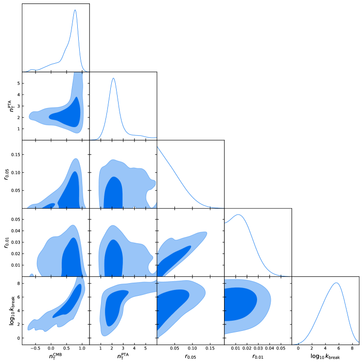
Figure 1: Marginalized posterior distributions of the parameters in the broken power-law model (2) of IGW with $n_{\text{T,CMB}}$ free.

Parameter	Best fit	68% limits
$r_{0.05}$	$0.0296$	$<0.0549\,(<0.107)$
$r_{0.01}$	$0.0141$	$<0.0199\,(<0.0338)$
$n^{\mathrm{CMB}}_{\mathrm{T}}$	$0.428$	$0.55^{+0.37}_{-0.10}$
$n^{\mathrm{PTA}}_{\mathrm{T}}$	$2.08$	$2.42^{+0.32}_{-0.91}$
$\log_{10}{k_{\mathrm{break}}}$	$4.19$	$5.0^{+2.0}_{-1.5}$

Table 1: The bestfit values and the 68% limit of posterior distributions of the parameters in the broken power-law model (2) of IGW with $n_{\text{T,CMB}}$ free. We also show the 95% limit for $r$ in parentheses.

The results are presented in Figure 1 and Table 1. As expected, the bestfit value $\log_{10}k_{\mathrm{break}}=4.19$, which is just between the CMB and PTA bands. The posterior of the spectral index $n^{\text{PTA}}_{\text{T}}$ at PTA band is $n^{\text{PTA}}_{\text{T}}\simeq 2$, in agreement with the results of NANOGrav NANOGrav:2023hvm ; Vagnozzi:2023lwo , since it is constrained mainly by the PTA itself. According to Equation 3, we have $P_{\text{T}}\sim rk^{n^{\text{PTA}}_{\text{T}}}k_{\text{break}}^{n^{\text{CMB}}_{\text{T}}-n^{\text{PTA}}_{\text{T}}}$ for fixed $k_{\text{pivot}}$, which suggests that $n^{\text{CMB}}_{\text{T}}$ is correlated positively with $\log_{10}{k_{\text{break}}}$, as showed in Figure 1.

The 95% upper limit of $r_{0.05}$ is $r_{0.05}<0.107$, higher than that of Planck+BK18 (e.g. $r\lesssim 0.03$ in Refs.BICEP:2021xfz ; Tristram:2021tvh ), while the 95% upper limit of $r_{0.01}$ is $r_{0.01}<0.0338$, However, this is a natural result, since for a blue-tilted IGW with the bestfit $n^{\text{CMB}}_{\text{T}}=0.428$, the amplitude of IGW must be lower at larger scale (smaller $k_{\text{pivot}}$). Accordingly, the constraint will be notably different at different $k_{pivot}\lesssim 0.05$ Mpc^-1.

However, it is significant to find that unlike that of NANOGrav NANOGrav:2023hvm at CMB band $n^{\text{CMB}}_{\text{T}}\simeq 2$ is not favored, instead $n^{\text{CMB}}_{\text{T}}=0.55^{+0.37}_{-0.10}$ with the bestfit $n^{\text{CMB}}_{\text{T}}=0.428$, while $n^{\text{CMB}}_{\text{T}}\simeq 0$ is still in the $95\%$ CL. range, which suggests that a slow-roll period of inflation at CMB band is not excluded. Thus it is interesting to see what if we fix $n^{\text{CMB}}_{\text{T}}=-r/8$.

III.2 $n^{\text{CMB}}_{\text{T}}=-r/8$

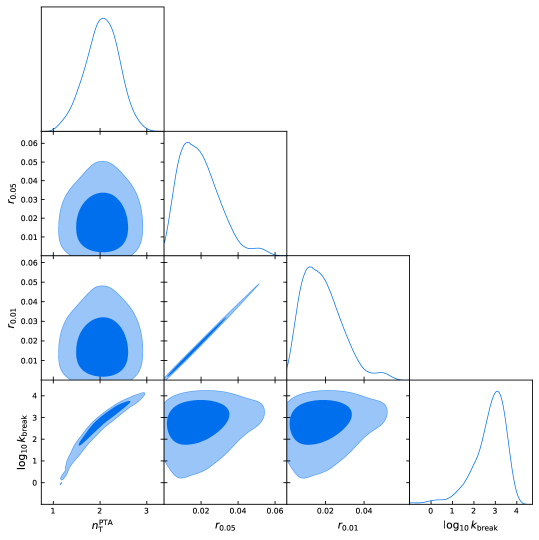
Figure 2: Marginalized posterior distributions of the parameters in the broken power-law model (2) with slow-roll $n_{\text{T,CMB}}$.

Parameter	Best fit	68% limits
$r_{0.05}$	$0.0091$	$0.0194^{+0.0069}_{-0.014}\,(^{+0.020}_{-0.019})$
$r_{0.01}$	$0.0086$	$0.0184^{+0.0065}_{-0.013}\,(^{+0.019}_{-0.018})$
$n^{\mathrm{PTA}}_{\mathrm{T}}$	$2.198$	$2.04^{+0.39}_{-0.34}$
$\log_{10}{k_{\mathrm{break}}}$	$3.01$	$2.72^{+0.92}_{-0.40}$

Table 2: The bestfit values and the 68% limit of posterior distributions of the parameters of the broken power-law model (2) with slow-roll $n_{\text{T,CMB}}$. We also show the 95% limit for $r$ in parentheses.

Next, we fix $n_{\text{T,CMB}}=-r/8$, i.e. standard slow-roll inflation is not broken at CMB scale. The results are presented in Figure 2 and Table 2. As expected, the broken scale is $k_{\text{break}}=2.72^{+0.92}_{-0.40}$, which is well between the CMB and PTA bands, and the posterior of the spectral index $n^{\text{PTA}}_{\text{T}}$ at PTA band is still $n^{\text{PTA}}_{\text{T}}\simeq 2$.

The 95% CL. range of $r$ is $r_{0.05}=0.019^{+0.020}_{-0.019}$, which is similar to that of $r_{0.01}$, since unlike in section III.A, we have $n^{\text{CMB}}_{\text{T}}=-r/8\simeq 0$ nearly scale-invariant. This upper limit, $r\lesssim 0.039$, is comparable with (but slightly higher than) that of Planck+BK18 BICEP:2021xfz ; Tristram:2021tvh . The bestfit $r$ is $r_{0.05}=0.0091$, however, it is unexpected that $r=0$ is at $2\sigma$ level. According to Equation 2, the bound on $r$ seems to be indirectly affect the NANOGrav results ($n^{\text{PTA}}_{\text{T}}$, $k_{\text{break}}$).

IV Discussion

IV.1 Conclusion

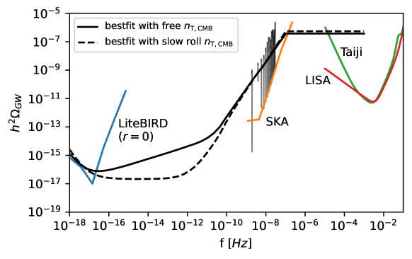
Figure 3: The bestfit energy spectrum $\Omega_{GW}(f)$ of IGWB with $n_{\text{T}}^{\text{CMB}}$ free and $n_{\text{T}}^{\text{CMB}}=-r/8$, respectively. We also show the sensitivity curves for LiteBIRD, SKA (Square Kilometre Array), space-based laser interferometers: LISA and Taiji. Here, we use the transfer function showed in Ref.Kite:2021yoe , which can return to Equation 4 at the high frequency limit, see also Refs.Turner:1993vb ; Boyle:2005se ; Zhao:2006mm ; Kuroyanagi:2014nba ; Liu:2015psa . As commented in section IV, when $f>10^{-7}$ the highly-blue ($n_{\text{T}}^{\text{PTA}}\simeq 2$) tilt needs to be cut off, though we plot $\Omega_{GW}(f>10^{-7})$ with a straight line, which but is actually model-dependent, e.g.Kuroyanagi:2020sfw ; Benetti:2021uea .

In conclusion, we find that though the bestfit spectral tilt of IGW at PTA band is $n^{\text{PTA}}_{\text{T}}\simeq 2$, unlike that of the NANOGrav NANOGrav:2023hvm $n^{\text{CMB}}_{\text{T}}\simeq 2$ is not favored at CMB band, instead the bestfit is $n^{\text{CMB}}_{\text{T}}=0.55^{+0.37}_{-0.10}$, while a detectable amplitude of $r$ with $n^{\text{CMB}}_{\text{T}}\simeq 0$ is still compatible. In particular if we fix $n^{\text{CMB}}_{\text{T}}=-r/8$ in light of standard slow-roll inflation, the upper bound on $r$ is $r\lesssim 0.039$, slightly higher than that of Planck+BK18 BICEP:2021xfz

In Figure 3, we show our bestfit energy spectrum $\Omega_{GW}(f)$ of IGWB with $n_{\text{T}}^{\text{CMB}}$ free and $n_{\text{T}}^{\text{CMB}}=-r/8$, respectively. The sensitivity curves for LiteBIRD and SKA are based on the results of Ref.Campeti:2020xwn . Here, our bestfit $\Omega_{GW}(f)$ covers the band at $f\sim 10^{-18}-10^{-8}$Hz, which naturally offers a guide for building relevant models of inflation and exploring new physics at corresponding band, since such a bestfit $\Omega_{GW}(f)$ can simultaneously explain current observations at both CMB and PTA bands.

However, beyond the PTA band the highly-blue ($n_{\text{T}}^{\text{PTA}}\simeq 2$) tilt must be cut off at certain $k_{cutoff}=2\pi f_{cutoff}$ to avoid the confliction with the BBN bound. In Figure 3, what is $P_{\text{T}}$ at $k>k_{cutoff}$ is not relevant with our MCMC results, which actually is model-dependent, e.g.Kuroyanagi:2020sfw ; Benetti:2021uea , see also discussion in section IV.B. Thus the spectrum of IGWB at that band is open, however, the space-based laser interferometers, LISA and Taiji, might detect the corresponding IGWB signal.

In next decade, with the accumulations of PTA and CMB data, SGWB at PTA band would be confirmed eventually, and also upcoming CMB observations, such as CMB-S4 CMB-S4:2020lpa , LiteBIRD Hazumi:2019lys would bring us more information on IGWB at CMB band. In view of this, our work is suggesting that a joint MCMC analysis of PTA and CMB data might be indispensable, which would open a unforeseen door into our very early Universe.

IV.2 Implications for inflation

It is interesting to see what our results will imply for inflation. As commented in Ref.Vagnozzi:2023lwo , a blue-tilted IGW suggests that inflation must violate null energy condition (NEC), i.e. $T_{\mu\nu}n^{\mu}n^{\nu}<0$ (equivalently ${\dot{H}}>0$ or $\epsilon=-{{\dot{H}}\over H^{2}}<0$), e.g.Piao:2004tq ; Piao:2003ty , see also Kobayashi:2010cm ; Kobayashi:2011nu , if the initial Bunch-Davis state of perturbation modes is not modified. Though it is not difficult to achieve $n^{\text{PTA}}_{\text{T}}\simeq 2$, which requires $\epsilon\ll-1$, e.g.Piao:2004jg ; Liu:2011ns , such a highly blue tilt of IGWB implies that inflation must end at a low scale NANOGrav:2023hvm ; Vagnozzi:2023lwo , or else it will be conflicted with the BBN bound on relativistic components.

However, it might be possible that the violation of NEC happened before a (standard) slow-roll inflation, so that the blue-tilted $P_{\text{T}}$ is cut off at certain $k_{cutoff}$ beyond the PTA band (when $k>k_{cutoff}$ the spectrum is flat). In corresponding models, the energy spectrum of IGW will be shown as the black solid $\Omega_{GW}(f)$ curve in Figure 3, and at CMB band for such a period of NEC violation the scale-invariant primordial scalar perturbation required by Planck observations can be harvested in light of Piao:2004tq ; Kobayashi:2010cm ; Piao:2010bi ; Liu:2011ns ; Liu:2012ww ; Nishi:2015pta ; Nishi:2016ljg .

It is also possible that the violation of NEC might be just short-lived, which happened between two (slow-roll) periods of inflation with $H\simeq H_{inf1}$ and a higher scale $H\simeq H_{inf2}\gg H_{inf1}$, respectively. In corresponding model Cai:2020qpu ; Cai:2022nqv ; Cai:2023uhc , we approximately have

$${P_{\text{T}}(k)}\sim{{{H}^{2}_{inf1}}+{\cal A}\left({k\over k_{cutoff}}\right)^{n_{\text{T}}^{\text{PTA}}}H^{2}_{inf2}\over 1+{\cal A}\left({k\over k_{cutoff}}\right)^{n_{\text{T}}^{\text{PTA}}}}\,,$$ (5)

where ${\cal A}={\Gamma^{2}(\nu)\over\pi}\left({2\nu-1\over 4}\right)^{1-2\nu}\sim{\cal O}(1)$ with $\nu=1/2+{1\over 1-\epsilon}$,

$$n_{\text{T}}^{\text{PTA}}=-{2\epsilon\over 1-\epsilon}\simeq 2,\quad for\quad\epsilon\ll 1.$$ (6)

According to Equation 5, we have $P_{\text{T}}\simeq H_{inf1}^{2}$ for $k/k_{cutoff}\ll({H_{inf1}\over H_{inf2}})^{2/n_{\text{T}}^{\text{PTA}}}\ll 1$ corresponding the CMB band, while $P_{\text{T}}\sim k^{n_{\text{T}}^{\text{PTA}}}\simeq k^{2}$ for $({H_{inf1}\over H_{inf2}})^{2/n_{\text{T}}^{\text{PTA}}}\ll k/k_{cutoff}\ll 1$ corresponding the PTA band. Thus when $k/k_{cutoff}\ll 1$, we have

$${P_{\text{T}}(k)}\sim{{H}^{2}_{inf1}}\left[1+{\cal A}\left({k\over k_{cutoff}}\right)^{n_{\text{T}}^{\text{PTA}}}{H^{2}_{inf2}\over{H}^{2}_{inf1}}\right]\,.$$ (7)

It is just Equation 2 for $k_{\rm break}\simeq k_{cutoff}({H_{inf1}\over H_{inf2}})^{2/n_{\text{T}}^{\text{PTA}}}$ and $n_{\text{T}}^{\text{CMB}}\simeq 0$. Thus the energy spectrum will be showed as the black dashed $\Omega_{GW}(f)$ curve in Figure 3. Here, $k_{cutoff}$ is a cutoff scale, see also section IV.A, beyond which $P_{\text{T}}\sim H_{inf2}^{2}$ is flat, or might be modified as in e.g. Refs.Kuroyanagi:2014nba ; Kuroyanagi:2020sfw ; Benetti:2021uea . Thus the IGWB at $k>k_{\text{cutoff}}$ ($f>10^{-7}$Hz in Figure 3) is model-dependent, which is unknown and needs to be explored, which suggests that the requirement of BBN that inflation must end at a low scale NANOGrav:2023hvm ; Vagnozzi:2023lwo is not workable.

It is also interesting to investigate other mechanisms, in which blue-tilted IGW at PTA band is sourced by other components during slow-roll inflation, such as the gauge fields Anber:2012du ; Cook:2011hg ; Mukohyama:2014gba ; Namba:2015gja ; Dimastrogiovanni:2016fuu ; Obata:2016oym ; Caldwell:2017chz , the non-Bunch-Davis initial states Ashoorioon:2014nta ; Choudhury:2023kam and the collisions of bubbles nucleated Li:2020cjj ; Wang:2018caj . In light of our MCMC results on $r$, $n_{\text{T}}^{\text{CMB}}$ and $n_{\text{T}}^{\text{PTA}}$, and also bestfit $\Omega_{GW}(f)$ in Figure 3, it is interesting to resurvey the relevant models.

References

- (1) A. H. Guth, The Inflationary Universe: A Possible Solution to the Horizon and Flatness Problems, Phys. Rev. D 23 (1981) 347–356.
- (2) A. D. Linde, A New Inflationary Universe Scenario: A Possible Solution of the Horizon, Flatness, Homogeneity, Isotropy and Primordial Monopole Problems, Phys. Lett. B 108 (1982) 389–393.
- (3) A. Albrecht and P. J. Steinhardt, Cosmology for Grand Unified Theories with Radiatively Induced Symmetry Breaking, Phys. Rev. Lett. 48 (1982) 1220–1223.
- (4) A. A. Starobinsky, A New Type of Isotropic Cosmological Models Without Singularity, Phys. Lett. B 91 (1980) 99–102.
- (5) A. D. Linde, Chaotic Inflation, Phys. Lett. B 129 (1983) 177–181.
- (6) M. Kamionkowski, A. Kosowsky, and A. Stebbins, Statistics of cosmic microwave background polarization, Phys. Rev. D 55 (1997) 7368–7388, [astro-ph/9611125].
- (7) M. Kamionkowski, A. Kosowsky, and A. Stebbins, A Probe of primordial gravity waves and vorticity, Phys. Rev. Lett. 78 (1997) 2058–2061, [astro-ph/9609132].
- (8) BICEP, Keck Collaboration, P. A. R. Ade et al., Improved Constraints on Primordial Gravitational Waves using Planck, WMAP, and BICEP/Keck Observations through the 2018 Observing Season, Phys. Rev. Lett. 127 (2021), no. 15 151301, [arXiv:2110.00483].
- (9) NANOGrav Collaboration, G. Agazie et al., The NANOGrav 15 yr Data Set: Evidence for a Gravitational-wave Background, Astrophys. J. Lett. 951 (2023), no. 1 L8, [arXiv:2306.16213].
- (10) J. Antoniadis et al., The second data release from the European Pulsar Timing Array III. Search for gravitational wave signals, arXiv:2306.16214.
- (11) D. J. Reardon et al., Search for an Isotropic Gravitational-wave Background with the Parkes Pulsar Timing Array, Astrophys. J. Lett. 951 (2023), no. 1 L6, [arXiv:2306.16215].
- (12) H. Xu et al., Searching for the Nano-Hertz Stochastic Gravitational Wave Background with the Chinese Pulsar Timing Array Data Release I, Res. Astron. Astrophys. 23 (2023), no. 7 075024, [arXiv:2306.16216].
- (13) NANOGrav Collaboration, A. Afzal et al., The NANOGrav 15 yr Data Set: Search for Signals from New Physics, Astrophys. J. Lett. 951 (2023), no. 1 L11, [arXiv:2306.16219].
- (14) H.-L. Huang, Y. Cai, J.-Q. Jiang, J. Zhang, and Y.-S. Piao, Supermassive primordial black holes in multiverse: for nano-Hertz gravitational wave and high-redshift JWST galaxies, arXiv:2306.17577.
- (15) P. F. Depta, K. Schmidt-Hoberg, and C. Tasillo, Do pulsar timing arrays observe merging primordial black holes?, arXiv:2306.17836.
- (16) S. Vagnozzi, Implications of the NANOGrav results for inflation, Mon. Not. Roy. Astron. Soc. 502 (2021), no. 1 L11–L15, [arXiv:2009.13432].
- (17) S. Vagnozzi, Inflationary interpretation of the stochastic gravitational wave background signal detected by pulsar timing array experiments, arXiv:2306.16912.
- (18) T. Ghosh, A. Ghoshal, H.-K. Guo, F. Hajkarim, S. F. King, K. Sinha, X. Wang, and G. White, Did we hear the sound of the Universe boiling? Analysis using the full fluid velocity profiles and NANOGrav 15-year data, arXiv:2307.02259.
- (19) X. Niu and M. H. Rahat, NANOGrav signal from axion inflation, arXiv:2307.01192.
- (20) R. A. Konoplya and A. Zhidenko, Asymptotic tails of massive gravitons in light of pulsar timing array observations, arXiv:2307.01110.
- (21) S.-P. Li and K.-P. Xie, A collider test of nano-Hertz gravitational waves from pulsar timing arrays, arXiv:2307.01086.
- (22) P. Di Bari and M. H. Rahat, The split majoron model confronts the NANOGrav signal, arXiv:2307.03184.
- (23) Q.-H. Zhu, Z.-C. Zhao, and S. Wang, Joint implications of BBN, CMB, and PTA Datasets for Scalar-Induced Gravitational Waves of Second and Third orders, arXiv:2307.03095.
- (24) X. K. Du, M. X. Huang, F. Wang, and Y. K. Zhang, Did the nHZ Gravitational Waves Signatures Observed By NANOGrav Indicate Multiple Sector SUSY Breaking?, arXiv:2307.02938.
- (25) G. Ye and A. Silvestri, Can the gravitational wave background feel wiggles in spacetime?, arXiv:2307.05455.
- (26) S. Balaji, G. Domènech, and G. Franciolini, Scalar-induced gravitational wave interpretation of PTA data: the role of scalar fluctuation propagation speed, arXiv:2307.08552.
- (27) Z. Zhang, C. Cai, Y.-H. Su, S. Wang, Z.-H. Yu, and H.-H. Zhang, Nano-Hertz gravitational waves from collapsing domain walls associated with freeze-in dark matter in light of pulsar timing array observations, arXiv:2307.11495.
- (28) Y.-S. Piao and Y.-Z. Zhang, Phantom inflation and primordial perturbation spectrum, Phys. Rev. D 70 (2004) 063513, [astro-ph/0401231].
- (29) Y.-S. Piao and E. Zhou, Nearly scale invariant spectrum of adiabatic fluctuations may be from a very slowly expanding phase of the universe, Phys. Rev. D 68 (2003) 083515, [hep-th/0308080].
- (30) Y.-S. Piao and Y.-Z. Zhang, The Primordial perturbation spectrum from various expanding and contracting phases, Phys. Rev. D 70 (2004) 043516, [astro-ph/0403671].
- (31) M. Baldi, F. Finelli, and S. Matarrese, Inflation with violation of the null energy condition, Phys. Rev. D 72 (2005) 083504, [astro-ph/0505552].
- (32) Z.-G. Liu, J. Zhang, and Y.-S. Piao, Phantom Inflation with A Steplike Potential, Phys. Lett. B 697 (2011) 407–411, [arXiv:1012.0673].
- (33) T. Kobayashi, M. Yamaguchi, and J. Yokoyama, G-inflation: Inflation driven by the Galileon field, Phys. Rev. Lett. 105 (2010) 231302, [arXiv:1008.0603].
- (34) T. Kobayashi, M. Yamaguchi, and J. Yokoyama, Generalized G-inflation: Inflation with the most general second-order field equations, Prog. Theor. Phys. 126 (2011) 511–529, [arXiv:1105.5723].
- (35) T. Fujita, S. Kuroyanagi, S. Mizuno, and S. Mukohyama, Blue-tilted Primordial Gravitational Waves from Massive Gravity, Phys. Lett. B 789 (2019) 215–219, [arXiv:1808.02381].
- (36) S. Endlich, A. Nicolis, and J. Wang, Solid Inflation, JCAP 10 (2013) 011, [arXiv:1210.0569].
- (37) D. Cannone, G. Tasinato, and D. Wands, Generalised tensor fluctuations and inflation, JCAP 01 (2015) 029, [arXiv:1409.6568].
- (38) W. Giarè, F. Renzi, and A. Melchiorri, Higher-Curvature Corrections and Tensor Modes, Phys. Rev. D 103 (2021), no. 4 043515, [arXiv:2012.00527].
- (39) Y. Cai, Y.-T. Wang, and Y.-S. Piao, Propagating speed of primordial gravitational waves and inflation, Phys. Rev. D 94 (2016), no. 4 043002, [arXiv:1602.05431].
- (40) Y. Cai, Y.-T. Wang, and Y.-S. Piao, Is there an effect of a nontrivial during inflation?, Phys. Rev. D 93 (2016), no. 6 063005, [arXiv:1510.08716].
- (41) Planck Collaboration, N. Aghanim et al., Planck 2018 results. VI. Cosmological parameters, Astron. Astrophys. 641 (2020) A6, [arXiv:1807.06209]. [Erratum: Astron.Astrophys. 652, C4 (2021)].
- (42) Planck Collaboration, Y. Akrami et al., Planck 2018 results. X. Constraints on inflation, Astron. Astrophys. 641 (2020) A10, [arXiv:1807.06211].
- (43) Y. Cai and Y.-S. Piao, Intermittent null energy condition violations during inflation and primordial gravitational waves, Phys. Rev. D 103 (2021), no. 8 083521, [arXiv:2012.11304].
- (44) H. W. H. Tahara and T. Kobayashi, Nanohertz gravitational waves from a null-energy-condition violation in the early universe, Phys. Rev. D 102 (2020), no. 12 123533, [arXiv:2011.01605].
- (45) Z.-G. Liu, J. Zhang, and Y.-S. Piao, A Galileon Design of Slow Expansion, Phys. Rev. D 84 (2011) 063508, [arXiv:1105.5713].
- (46) Z.-G. Liu and Y.-S. Piao, A Galileon Design of Slow Expansion: Emergent universe, Phys. Lett. B 718 (2013) 734–739, [arXiv:1207.2568].
- (47) S. Nishi and T. Kobayashi, Generalized Galilean Genesis, JCAP 03 (2015) 057, [arXiv:1501.02553].
- (48) S. Nishi and T. Kobayashi, Scale-invariant perturbations from null-energy-condition violation: A new variant of Galilean genesis, Phys. Rev. D 95 (2017), no. 6 064001, [arXiv:1611.01906].
- (49) S. Kuroyanagi, T. Takahashi, and S. Yokoyama, Blue-tilted Tensor Spectrum and Thermal History of the Universe, JCAP 02 (2015) 003, [arXiv:1407.4785].
- (50) S. Kuroyanagi, T. Takahashi, and S. Yokoyama, Blue-tilted inflationary tensor spectrum and reheating in the light of NANOGrav results, JCAP 01 (2021) 071, [arXiv:2011.03323].
- (51) M. Benetti, L. L. Graef, and S. Vagnozzi, Primordial gravitational waves from NANOGrav: A broken power-law approach, Phys. Rev. D 105 (2022), no. 4 043520, [arXiv:2111.04758].
- (52) W. G. Lamb, S. R. Taylor, and R. van Haasteren, The Need For Speed: Rapid Refitting Techniques for Bayesian Spectral Characterization of the Gravitational Wave Background Using PTAs, arXiv:2303.15442.
- (53) G. Ye, B. Hu, and Y.-S. Piao, Implication of the Hubble tension for the primordial Universe in light of recent cosmological data, Phys. Rev. D 104 (2021), no. 6 063510, [arXiv:2103.09729].
- (54) G. Ye and Y.-S. Piao, Is the Hubble tension a hint of AdS phase around recombination?, Phys. Rev. D 101 (2020), no. 8 083507, [arXiv:2001.02451].
- (55) J.-Q. Jiang and Y.-S. Piao, Toward early dark energy and ns=1 with Planck, ACT, and SPT observations, Phys. Rev. D 105 (2022), no. 10 103514, [arXiv:2202.13379].
- (56) J.-Q. Jiang, G. Ye, and Y.-S. Piao, Return of Harrison-Zeldovich spectrum in light of recent cosmological tensions, arXiv:2210.06125.
- (57) D. Blas, J. Lesgourgues, and T. Tram, The Cosmic Linear Anisotropy Solving System (CLASS) II: Approximation schemes, JCAP 07 (2011) 034, [arXiv:1104.2933].
- (58) J. Torrado and A. Lewis, Cobaya: Code for Bayesian Analysis of hierarchical physical models, JCAP 05 (2021) 057, [arXiv:2005.05290].
- (59) K. Saikawa and S. Shirai, Precise WIMP Dark Matter Abundance and Standard Model Thermodynamics, JCAP 08 (2020) 011, [arXiv:2005.03544].
- (60) M. Tristram et al., Improved limits on the tensor-to-scalar ratio using BICEP and Planck data, Phys. Rev. D 105 (2022), no. 8 083524, [arXiv:2112.07961].
- (61) T. Kite, J. Chluba, A. Ravenni, and S. P. Patil, Clarifying transfer function approximations for the large-scale gravitational wave background in CDM, Mon. Not. Roy. Astron. Soc. 509 (2021), no. 1 1366–1376, [arXiv:2107.13351].
- (62) M. S. Turner, M. J. White, and J. E. Lidsey, Tensor perturbations in inflationary models as a probe of cosmology, Phys. Rev. D 48 (1993) 4613–4622, [astro-ph/9306029].
- (63) L. A. Boyle and P. J. Steinhardt, Probing the early universe with inflationary gravitational waves, Phys. Rev. D 77 (2008) 063504, [astro-ph/0512014].
- (64) W. Zhao and Y. Zhang, Relic gravitational waves and their detection, Phys. Rev. D 74 (2006) 043503, [astro-ph/0604458].
- (65) X.-J. Liu, W. Zhao, Y. Zhang, and Z.-H. Zhu, Detecting Relic Gravitational Waves by Pulsar Timing Arrays: Effects of Cosmic Phase Transitions and Relativistic Free-Streaming Gases, Phys. Rev. D 93 (2016), no. 2 024031, [arXiv:1509.03524].
- (66) P. Campeti, E. Komatsu, D. Poletti, and C. Baccigalupi, Measuring the spectrum of primordial gravitational waves with CMB, PTA and Laser Interferometers, JCAP 01 (2021) 012, [arXiv:2007.04241].
- (67) CMB-S4 Collaboration, K. Abazajian et al., CMB-S4: Forecasting Constraints on Primordial Gravitational Waves, Astrophys. J. 926 (2022), no. 1 54, [arXiv:2008.12619].
- (68) M. Hazumi et al., LiteBIRD: A Satellite for the Studies of B-Mode Polarization and Inflation from Cosmic Background Radiation Detection, J. Low Temp. Phys. 194 (2019), no. 5-6 443–452.
- (69) Y.-S. Piao, Adiabatic Spectra During Slowly Evolving, Phys. Lett. B 701 (2011) 526–529, [arXiv:1012.2734].
- (70) Y. Cai and Y.-S. Piao, Generating enhanced primordial GWs during inflation with intermittent violation of NEC and diminishment of GW propagating speed, JHEP 06 (2022) 067, [arXiv:2201.04552].
- (71) Y. Cai, M. Zhu, and Y.-S. Piao, Primordial black holes from null energy condition violation during inflation, arXiv:2305.10933.
- (72) M. M. Anber and L. Sorbo, Non-Gaussianities and chiral gravitational waves in natural steep inflation, Phys. Rev. D 85 (2012) 123537, [arXiv:1203.5849].
- (73) J. L. Cook and L. Sorbo, Particle production during inflation and gravitational waves detectable by ground-based interferometers, Phys. Rev. D 85 (2012) 023534, [arXiv:1109.0022]. [Erratum: Phys.Rev.D 86, 069901 (2012)].
- (74) S. Mukohyama, R. Namba, M. Peloso, and G. Shiu, Blue Tensor Spectrum from Particle Production during Inflation, JCAP 08 (2014) 036, [arXiv:1405.0346].
- (75) R. Namba, M. Peloso, M. Shiraishi, L. Sorbo, and C. Unal, Scale-dependent gravitational waves from a rolling axion, JCAP 01 (2016) 041, [arXiv:1509.07521].
- (76) E. Dimastrogiovanni, M. Fasiello, and T. Fujita, Primordial Gravitational Waves from Axion-Gauge Fields Dynamics, JCAP 01 (2017) 019, [arXiv:1608.04216].
- (77) I. Obata, Chiral primordial blue tensor spectra from the axion-gauge couplings, JCAP 06 (2017) 050, [arXiv:1612.08817].
- (78) R. R. Caldwell and C. Devulder, Axion Gauge Field Inflation and Gravitational Leptogenesis: A Lower Bound on B Modes from the Matter-Antimatter Asymmetry of the Universe, Phys. Rev. D 97 (2018), no. 2 023532, [arXiv:1706.03765].
- (79) A. Ashoorioon, K. Dimopoulos, M. M. Sheikh-Jabbari, and G. Shiu, Non-Bunch–Davis initial state reconciles chaotic models with BICEP and Planck, Phys. Lett. B 737 (2014) 98–102, [arXiv:1403.6099].
- (80) S. Choudhury, Single field inflation in the light of NANOGrav 15-year Data: Quintessential interpretation of blue tilted tensor spectrum through Non-Bunch Davies initial condition, arXiv:2307.03249.
- (81) H.-H. Li, G. Ye, and Y.-S. Piao, Is the NANOGrav signal a hint of dS decay during inflation?, Phys. Lett. B 816 (2021) 136211, [arXiv:2009.14663].
- (82) Y.-T. Wang, Y. Cai, and Y.-S. Piao, Phase-transition sound of inflation at gravitational waves detectors, Phys. Lett. B 789 (2019) 191–196, [arXiv:1801.03639].