Scaling in local to global condensation of wealth on sparse networks

Hyun Gyu Lee supersting85@kias.re.kr School of Computational Sciences, Korea Institute for Advanced Study, Seoul 02455, Korea    Deok-Sun Lee deoksunlee@kias.re.kr School of Computational Sciences, Korea Institute for Advanced Study, Seoul 02455, Korea Center for AI and Natural Sciences, Korea Institute for Advanced Study, Seoul 02455, Korea
(February 28, 2024)
Abstract

The prevalence of wealth inequality propels us to characterize its origin and progression, via empirical and theoretical studies. The Yard-Sale(YS) model, in which a portion of the smaller wealth is transferred between two individuals, culminates in the concentration of almost all wealth to a single individual, while distributing rest of the wealth with a power-law of exponent one. By incorporating redistribution to the model, in which the transferred wealth is proportional to the sender’s wealth, we show that such extreme inequality is suppressed if the frequency ratio of redistribution to the YS-type exchange exceeds the inverse of the population size. Studying our model on a sparsely-connected population, we find that the wealth inequality ceases to grow for a period, when local rich nodes can no longer acquire wealth from their broke nearest neighbors. Subsequently, inequality resumes growth due to the redistribution effect by allowing locally amassed wealth to move and coalesce. Analyzing the Langevin equations and the coalescing random walk on complex networks, we elucidate the scaling behaviors of wealth inequality in those multiple phases. These findings reveal the influence of network structure on wealth distribution, offering a novel perspective on wealth inequality.

I Introduction

Wealth inequality may be attributed to numerous socioeconomic factors and their orchestration. Yet the universal power-law wealth and income distributions Pareto (1897); Levy and Solomon (1996); Gabaix (2009) imply a common mechanism at play, and the possibility of understanding how wealth inequality has arisen and how long it will persist  Piketty (2017); Chancel and Piketty (2021); Chancel et al. (2022). Given that individuals participating in a trade can undergo wealth transfer due to imperfect pricing, various wealth exchange models have been studied extensively, and their steady-state solutions, often available analytically, serve as plausible explanations for various wealth distributions Ispolatov et al. (1998); Bouchaud and Mézard (2000); Dragulescu and Yakovenko (2000); Samanidou et al. (2007); Yakovenko and Rosser Jr. (2009); Cha et al. (2010); Barbier and Lee (2017).

The Yard-Sale(YS) model  Chakraborti and Chakrabarti (2000); Hayes (2002) is remarkable as it generates an extreme wealth inequality from a seemingly fair (and thus realistic) exchange rule: A fraction of the sender’s and receiver’s smaller wealth is transferred in each trade, and ultimately, almost all wealth is concentrated in a single individual while the remaining wealth is distributed by a power-law with exponent one across the rest of the population Boghosian (2014). The model’s simplicity and yet the emergence of such stark inequality have attracted much attention Chakraborti (2002); Sinha (2003); Moukarzel et al. (2007); Moukarzel (2011); Bustos-Guajardo and Moukarzel (2012); Boghosian (2014); Boghosian et al. (2017). The Gini index is a Lyapunov functional, never decreasing with time, in the YS model Boghosian et al. (2017) and in a class of models Cardoso et al. (2023). However, such global wealth condensation does not yet happen in the real world; The present era may be shorter than the condensation time scale.

The degree of real-world wealth inequality has been changing with time Piketty (2017); Chancel and Piketty (2021); Chancel et al. (2022). In this light, the non-stationary, rather than stationary, state of a model may offer a better explanation of the reality. Also, by relaxing constraints like the fully-connected population often assumed in many studies and by considering multiple modes of wealth exchange, the YS model can become more realistic and reveal a richer set of insights. For example, transferring a fraction of the sender’s wealth, occurring in donation, investment, or taxation and also called the loser rule Hayes (2002); Cardoso et al. (2020), effectively redistributes wealth and suppresses wealth inequality Ispolatov et al. (1998); Bouchaud and Mézard (2000); Dragulescu and Yakovenko (2000); Sinha (2003) while there can be various ways to achieve redistribution Cardoso et al. (2020). Investigating the non-stationary state of the generalized YS model Boghosian (2014); Boghosian et al. (2017) which allows such redistribution (RD) mode of wealth transfer, as well as the YS-mode, between connected pairs in a structured population Bustos-Guajardo and Moukarzel (2012), we identify new factors influencing wealth inequality and provide a novel theoretical framework.

We show that the extreme inequality of the original YS model in the long-time limit can be suppressed by increasing the ratio of the RD-mode transfers beyond the inverse of the population size. In the sparsely-connected population, inequality evolves with time through multiple phases, and we elucidate the underlying mechanisms. Initially, the inequality grows primarily driven by the YS-mode transfers before saturating over a period of time due to depleted wealth of the nearest neighbors of locally rich nodes. We call this stage local condensate phase. As time passes, the RD-mode transfer effectively thaws this frozen state, enabling further elevation of inequality via random walk and coalescence of locally-concentrated wealth. In these stages, wealth inequality exhibits scaling behaviors, which we show originate from the correlation between wealth and connectivity of individuals. This demonstrates the critical role of the structure of networks in shaping the wealth distribution. Finally, comparing with the empirical data, we discuss the implications of our findings.

II Model

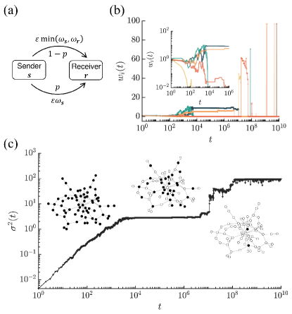
We consider a network of N𝑁N nodes (individuals) connected by L𝐿L undirected links (trade partnership) with the adjacency matrix Aij=0,1subscript𝐴𝑖𝑗01A_{ij}=0,1. Each node i𝑖i has wealth ωi(t)subscript𝜔𝑖𝑡\omega_{i}(t) with ωi(0)=1subscript𝜔𝑖01\omega_{i}(0)=1 initially. For every pair of connected nodes with rate N/L𝑁𝐿N/L, the sender (‘s’) and the receiver (‘r’) are determined randomly and the sender sends an amount ΔωΔ𝜔\Delta\omega of wealth to the receiver [Fig. 1 (a)], where ΔωΔ𝜔\Delta\omega is a fraction ε𝜀\varepsilon of either the smaller wealth or the sender’s wealth as

Δω={εmin{ωs,ωr}withprob. 1p(YSmode),εωswithprob.p(RDmode).Δ𝜔cases𝜀subscript𝜔ssubscript𝜔rwithprob.1𝑝YSmode𝜀subscript𝜔sformulae-sequencewithprob𝑝RDmode\Delta\omega=\begin{cases}\varepsilon\,\min\{\omega_{\rm s},\omega_{\rm r}\}&\ {\rm with}\ {\rm prob.}\ 1-p\ ({\rm YS\ mode}),\\ \varepsilon\,\omega_{\rm s}&\ {\rm with}\ {\rm prob.}\ p\ ({\rm RD\ mode}).\end{cases} (1)

Consequently their wealth change as (ωs,ωr)(ωsΔω,ωr+Δω)subscript𝜔ssubscript𝜔rsubscript𝜔sΔ𝜔subscript𝜔rΔ𝜔(\omega_{\rm s},\omega_{\rm r})\to(\omega_{\rm s}-\Delta\omega,\omega_{\rm r}+\Delta\omega) while their sum is preserved. The mean wealth is fixed, i.e., ω¯N1iωi(t)=1¯𝜔superscript𝑁1subscript𝑖subscript𝜔𝑖𝑡1\overline{\omega}\equiv N^{-1}\sum_{i}\omega_{i}(t)=1. We use x¯=N1j=1Nxj¯𝑥superscript𝑁1superscriptsubscript𝑗1𝑁subscript𝑥𝑗\overline{x}=N^{-1}\sum_{j=1}^{N}x_{j} to denote the spatial average. The parameter p𝑝p is the relative ratio of the RD-mode transfers. This is a network version of the model introduced in Refs. Boghosian (2014); Boghosian et al. (2017). For the underlying networks, we use the complete graphs (Aij=1subscript𝐴𝑖𝑗1A_{ij}=1 for all ij𝑖𝑗i\neq j) and the giant connected components of sparse scale-free (SF) networks Barabási and Albert (1999) constructed by the static model Goh et al. (2001); Lee et al. (2004), which display power-law degree distributions Pdeg(k)N1iδki,kkγsubscript𝑃deg𝑘superscript𝑁1subscript𝑖subscript𝛿subscript𝑘𝑖𝑘similar-tosuperscript𝑘𝛾P_{\rm deg}(k)\equiv N^{-1}\sum_{i}\delta_{k_{i},k}\sim k^{-\gamma} for large k𝑘k with the degree ki=jAijsubscript𝑘𝑖subscript𝑗subscript𝐴𝑖𝑗k_{i}=\sum_{j}A_{ij} meaning the number of the nearest neighbors and γ𝛾\gamma called the degree exponent, and have the mean degree k¯=2L/N¯𝑘2𝐿𝑁\overline{k}=2L/N finite. Note that for a unit time interval, every pair of nodes is selected 2k¯2¯𝑘{2\over\overline{k}} times on the average for the transaction in Eq. (1).
Refer to caption
Figure 1: Model and its Monte-Carlo simulation results. (a) Two modes of wealth transfers in Eq. (1). (b) Time-evolution of individual wealth in a single run of simulation with p=106𝑝superscript106p=10^{-6} and ε=0.05𝜀0.05\varepsilon=0.05 on a SF network of N=97𝑁97N=97 nodes, L=200𝐿200L=200 links and the degree exponent γ=2.5𝛾2.5\gamma=2.5. Inset: The same plots for 1t1061𝑡superscript1061\leq t\leq 10^{6}. (c) Time-evolution of wealth variance from the same simulation. Three insets represent a part of the network at t=102𝑡superscript102t=10^{2}, 105superscript10510^{5}, and 1010superscript101010^{10}, respectively, with rich (poor) nodes colored black (white).

For a measure of wealth inequality we use the wealth variance σ2(t)1Ni=1N(ωi(t)ω¯)2,superscript𝜎2𝑡1𝑁superscriptsubscript𝑖1𝑁superscriptsubscript𝜔𝑖𝑡¯𝜔2\sigma^{2}(t)\equiv\frac{1}{N}\sum_{i=1}^{N}(\omega_{i}(t)-\overline{\omega})^{2}, the second cumulant of the wealth distribution P(ω,t)𝑃𝜔𝑡P(\omega,t). A single run of the model simulation with small p𝑝p readily reveals multiple phases in the time-evolution of wealth inequality. See Figs. 1(b) and 1(c). i) In the early-time regime, for t104less-than-or-similar-to𝑡superscript104t\lesssim 10^{4}, individuals’ wealth is made increasingly different from one another, so wealth inequality grows. ii) Then a frozen period follows (104t107less-than-or-similar-tosuperscript104𝑡less-than-or-similar-tosuperscript10710^{4}\lesssim t\lesssim 10^{7}), when ωisubscript𝜔𝑖\omega_{i}’s and σ2superscript𝜎2\sigma^{2} hardly change with time. Rich nodes, with at least mean wealth (ω1𝜔1\omega\geq 1), are surrounded by the poor nearest neighbors having ω<1𝜔1\omega<1. With p=0𝑝0p=0, this local condensate phase becomes the equilibrium Bustos-Guajardo and Moukarzel (2012). iii) For 107t108less-than-or-similar-tosuperscript107𝑡less-than-or-similar-tosuperscript10810^{7}\lesssim t\lesssim 10^{8}, the wealth variance resumes growing and each locally-concentrated wealth switches its host to one of its nearest neighbors repeatedly, appearing to perform a random walk, until it encounters another local wealth and they coalesce Lee . iv) In the late-time regime (t108greater-than-or-equivalent-to𝑡superscript108t\gtrsim 10^{8}), global condensation occurs; almost all wealth is concentrated onto a single node. Yet its host changes with time and σ2superscript𝜎2\sigma^{2} fluctuates though weakly.

III Early and late-time regime: Analytic results

To understand these observations quantitatively and proceed, we construct the Langevin equation. In the mean-field approximation, it provides analytic results for the wealth variance and distribution in the early and late-time regime.

III.1 Langevin equation

In our model, at each discrete time step τ𝜏\tau, a pair of connected nodes (i,j𝑖𝑗i,j) are selected among L𝐿L pairs and performs the YS-mode transfer with probability 1p1𝑝1-p or the RD-mode transfer with probability p𝑝p. The node i𝑖i or j𝑗j becomes the sender with equal probability. Therefore the expected change of the wealth ωisubscript𝜔𝑖\omega_{i} of a node i𝑖i for the period from τ0subscript𝜏0\tau_{0} to τ0+Δτsubscript𝜏0Δ𝜏\tau_{0}+\Delta\tau is given by

ΔωiΔsubscript𝜔𝑖\displaystyle\Delta\omega_{i} {ωi(τ0+Δτ)ωi(τ0)}absentdelimited-⟨⟩subscript𝜔𝑖subscript𝜏0Δ𝜏subscript𝜔𝑖subscript𝜏0\displaystyle\equiv\langle\{\omega_{i}(\tau_{0}+\Delta\tau)-\omega_{i}(\tau_{0})\}\rangle
=εj=1NAij[pΔτLωjωi2+pΔτLωi+ωj2ηij\displaystyle=\varepsilon\sum_{j=1}^{N}A_{ij}\biggl{[}p\frac{\Delta\tau}{L}\frac{\omega_{j}-\omega_{i}}{2}+\sqrt{p\frac{\Delta\tau}{L}}\frac{\omega_{i}+\omega_{j}}{2}\eta_{ij}
+(1p)ΔτLmin(ωi,ωj)ξij]\displaystyle+\sqrt{(1-p)\frac{\Delta\tau}{L}}\min{(\omega_{i},\omega_{j})}\xi_{ij}\biggr{]} (2)

with the continuous random variables ηijsubscript𝜂𝑖𝑗\eta_{ij} and ξijsubscript𝜉𝑖𝑗\xi_{ij} satisfying ηij=ξij=0delimited-⟨⟩subscript𝜂𝑖𝑗delimited-⟨⟩subscript𝜉𝑖𝑗0\langle\eta_{ij}\rangle=\langle\xi_{ij}\rangle=0, ηij2=ξij2=1delimited-⟨⟩superscriptsubscript𝜂𝑖𝑗2delimited-⟨⟩superscriptsubscript𝜉𝑖𝑗21\langle\eta_{ij}^{2}\rangle=\langle\xi_{ij}^{2}\rangle=1, ηij=ηjisubscript𝜂𝑖𝑗subscript𝜂𝑗𝑖\eta_{ij}=-\eta_{ji}, and ξij=ξjisubscript𝜉𝑖𝑗subscript𝜉𝑗𝑖\xi_{ij}=-\xi_{ji}. We use delimited-⟨⟩\langle\cdots\rangle to represent the ensemble average. Introducing (continuous) time tτN𝑡𝜏𝑁t\equiv\frac{\tau}{N} and taking large-N𝑁N limit, we find

dωi=𝑑subscript𝜔𝑖absent\displaystyle d\omega_{i}= εpk¯jLijωjdt+ε2pk¯jAijωi+ωj2dCij𝜀𝑝¯𝑘subscript𝑗subscript𝐿𝑖𝑗subscript𝜔𝑗𝑑𝑡𝜀2𝑝¯𝑘subscript𝑗subscript𝐴𝑖𝑗subscript𝜔𝑖subscript𝜔𝑗2𝑑subscript𝐶𝑖𝑗\displaystyle-\frac{\varepsilon p}{\overline{k}}\sum_{j}L_{ij}\omega_{j}dt+\varepsilon\sqrt{\frac{2p}{\overline{k}}}\sum_{j}A_{ij}\frac{\omega_{i}+\omega_{j}}{2}dC_{ij}
+ε2(1p)k¯jAijmin(ωi,ωj)dBij,𝜀21𝑝¯𝑘subscript𝑗subscript𝐴𝑖𝑗subscript𝜔𝑖subscript𝜔𝑗𝑑subscript𝐵𝑖𝑗\displaystyle+\varepsilon\sqrt{\frac{2(1-p)}{\overline{k}}}\sum_{j}A_{ij}\min{(\omega_{i},\omega_{j})}dB_{ij}, (3)

where LijkiδijAijsubscript𝐿𝑖𝑗subscript𝑘𝑖subscript𝛿𝑖𝑗subscript𝐴𝑖𝑗L_{ij}\equiv k_{i}\delta_{ij}-A_{ij} is the Laplacian, dBij𝑑subscript𝐵𝑖𝑗dB_{ij} and dCij𝑑subscript𝐶𝑖𝑗dC_{ij} are the Wiener processes satisfying dBij=dCij=0delimited-⟨⟩𝑑subscript𝐵𝑖𝑗delimited-⟨⟩𝑑subscript𝐶𝑖𝑗0\langle dB_{ij}\rangle=\langle dC_{ij}\rangle=0, dBij2=dCij2=dtdelimited-⟨⟩𝑑superscriptsubscript𝐵𝑖𝑗2delimited-⟨⟩𝑑superscriptsubscript𝐶𝑖𝑗2𝑑𝑡\langle dB_{ij}^{2}\rangle=\langle dC_{ij}^{2}\rangle=dt, dBij=dBji𝑑subscript𝐵𝑖𝑗𝑑subscript𝐵𝑗𝑖dB_{ij}=-dB_{ji}, and dCij=dCji𝑑subscript𝐶𝑖𝑗𝑑subscript𝐶𝑗𝑖dC_{ij}=-dC_{ji}. To fulfill the condition idωi=0subscript𝑖𝑑subscript𝜔𝑖0\sum_{i}d\omega_{i}=0, we adopted Ito^^𝑜\hat{o}’s scheme.

To proceed, we approximate the sum of the YS- and RD-mode transfers with all the nearest neighbors as 1k¯jAijωi+ωj2dCijD(RD)(ωi)dXisimilar-to-or-equals1¯𝑘subscript𝑗subscript𝐴𝑖𝑗subscript𝜔𝑖subscript𝜔𝑗2𝑑subscript𝐶𝑖𝑗superscript𝐷RDsubscript𝜔𝑖𝑑subscript𝑋𝑖\sqrt{\frac{1}{\overline{k}}}\sum_{j}A_{ij}\frac{\omega_{i}+\omega_{j}}{2}dC_{ij}\simeq\sqrt{D^{\rm(RD)}(\omega_{i})}dX_{i} and 1k¯jAijmin(ωi,ωj)dBijD(YS)(ωi)dYisimilar-to-or-equals1¯𝑘subscript𝑗subscript𝐴𝑖𝑗subscript𝜔𝑖subscript𝜔𝑗𝑑subscript𝐵𝑖𝑗superscript𝐷YSsubscript𝜔𝑖𝑑subscript𝑌𝑖\sqrt{\frac{1}{\overline{k}}}\sum_{j}A_{ij}\min{(\omega_{i},\omega_{j})}dB_{ij}\simeq\sqrt{D^{\rm(YS)}(\omega_{i})}dY_{i}, where dXi𝑑subscript𝑋𝑖dX_{i} and dYi𝑑subscript𝑌𝑖dY_{i} are the Wiener processes satisfying dXi=dYi=0delimited-⟨⟩𝑑subscript𝑋𝑖delimited-⟨⟩𝑑subscript𝑌𝑖0\langle dX_{i}\rangle=\langle dY_{i}\rangle=0, dXi2=dYi2=dtdelimited-⟨⟩𝑑superscriptsubscript𝑋𝑖2delimited-⟨⟩𝑑superscriptsubscript𝑌𝑖2𝑑𝑡\langle dX_{i}^{2}\rangle=\langle dY_{i}^{2}\rangle=dt. The coefficients D(RD)(ω)=k¯1j=1NAij{(ωi+ω)/2}2superscript𝐷RD𝜔delimited-⟨⟩superscript¯𝑘1superscriptsubscript𝑗1𝑁subscript𝐴𝑖𝑗superscriptsubscript𝜔𝑖𝜔22D^{\rm(RD)}(\omega)=\left\langle\overline{k}^{-1}\sum_{j=1}^{N}A_{ij}\{(\omega_{i}+\omega)/2\}^{2}\right\rangle and D(YS)(ω)=k¯1j=1NAijmin{ω,ωj}2D^{\rm(YS)}(\omega)=\left\langle\overline{k}^{-1}\sum_{j=1}^{N}A_{ij}\min\{\omega,\omega_{j}\}^{2}\right\rangle are the mean square of the transferred wealth for node i𝑖i under the RD and YS mode and given approximately by

D(RD)(ω)superscript𝐷RD𝜔\displaystyle D^{\rm(RD)}(\omega) {(ωi+ω)/2}2¯{ω2¯4forω0,ω24forω,similar-to-or-equalsabsentdelimited-⟨⟩¯superscriptsubscript𝜔𝑖𝜔22similar-to-or-equalscasesdelimited-⟨⟩¯superscript𝜔24for𝜔0superscript𝜔24for𝜔\displaystyle\simeq\langle\overline{\{(\omega_{i}+\omega)/2\}^{2}}\rangle\simeq\begin{cases}{\langle\overline{\omega^{2}}\rangle\over 4}&{\rm for}\ \omega\to 0,\\ {\omega^{2}\over 4}&{\rm for}\ \omega\to\infty,\end{cases} (4)
D(YS)(ω)superscript𝐷YS𝜔\displaystyle D^{\rm(YS)}(\omega) min{ωi,ω}2¯{ω2forω0,ω2¯forω.\displaystyle\simeq\langle\overline{\min\{\omega_{i},\omega\}^{2}}\rangle\simeq\begin{cases}\omega^{2}&{\rm for}\ \omega\to 0,\\ \langle\overline{\omega^{2}}\rangle&{\rm for}\ \omega\to\infty.\end{cases} (5)

Also note that D(RD)(ω)1similar-to-or-equalssuperscript𝐷RD𝜔1D^{\rm(RD)}(\omega)\simeq 1 and D(YS)(ω)1similar-to-or-equalssuperscript𝐷YS𝜔1D^{\rm(YS)}(\omega)\simeq 1 for ω𝜔\omega close to the initial value 111 in the early-time regime when all nodes have wealth close to 111. Finally, the Langevin equation for the wealth of a node is represented as

dωi=𝑑subscript𝜔𝑖absent\displaystyle d\omega_{i}= εpk¯jLijωjdt+ε2pD(RD)(ωi)dXi𝜀𝑝¯𝑘subscript𝑗subscript𝐿𝑖𝑗subscript𝜔𝑗𝑑𝑡𝜀2𝑝superscript𝐷RDsubscript𝜔𝑖𝑑subscript𝑋𝑖\displaystyle-\frac{\varepsilon\,p}{\overline{k}}\sum_{j}L_{ij}\omega_{j}dt+\varepsilon\sqrt{2p\,D^{\rm(RD)}(\omega_{i})}\,dX_{i}
+ε2(1p)D(YS)(ωi)dYi,𝜀21𝑝superscript𝐷YSsubscript𝜔𝑖𝑑subscript𝑌𝑖\displaystyle+\varepsilon\sqrt{2(1-p)\,D^{\rm(YS)}(\omega_{i})}\,dY_{i}, (6)

where dXi𝑑subscript𝑋𝑖dX_{i} and dYi𝑑subscript𝑌𝑖dY_{i} are the Wiener processes with mean 00 and variance dt𝑑𝑡dt representing the stochasticity of whether to send or receive wealth, and the coefficients D(RD)(ωi)superscript𝐷RDsubscript𝜔𝑖D^{\rm(RD)}(\omega_{i}) and D(YS)(ωi)superscript𝐷YSsubscript𝜔𝑖D^{\rm(YS)}(\omega_{i}) are given in Eq. (5). The first and second terms represent the deterministic and stochastic changes by the RD-mode transfers, and the third one from the YS transfers.

III.2 Wealth variance
Refer to caption
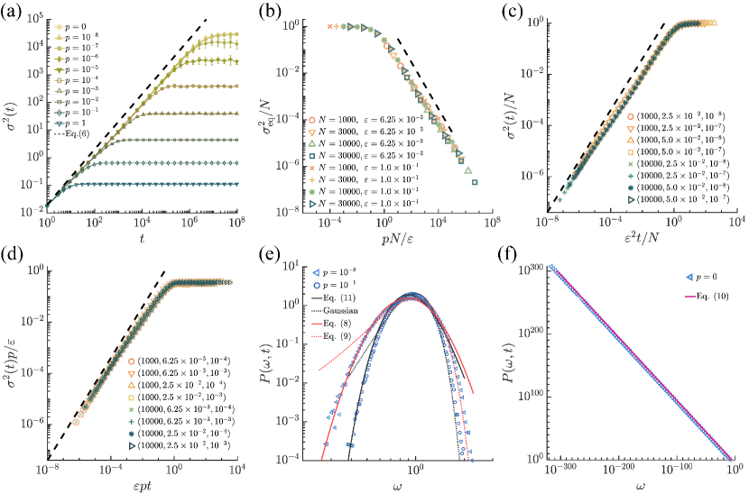
Figure 2: Wealth variance and distribution on the complete graphs. (a) Wealth variance for ε=0.1𝜀0.1\varepsilon=0.1 and different p𝑝p’s with N=105𝑁superscript105N=10^{5} averaged over 20 realization. (b) Data collapse of the rescaled wealth variance in the equilibrium state for different p𝑝p’s, ε𝜀\varepsilon’s and N𝑁N’s. The dashed line has slope 11-1. (c) Plots of σ2/Nsuperscript𝜎2𝑁\sigma^{2}/N versus ε2t/Nsuperscript𝜀2𝑡𝑁\varepsilon^{2}t/N for the parameters satisfying p<0.1p𝑝0.1subscript𝑝p<0.1p_{*} with pεNsubscript𝑝𝜀𝑁p_{*}\equiv{\varepsilon\over N}. Legends represent (N,ε,p)𝑁𝜀𝑝(N,\varepsilon,p). (d) Plot of σ2p/εsuperscript𝜎2𝑝𝜀\sigma^{2}p/\varepsilon versus εpt𝜀𝑝𝑡\varepsilon pt for the parameters satisfying p>p𝑝subscript𝑝p>p_{*}. (e) Wealth distributions with different p𝑝p’s for N=105𝑁superscript105N=10^{5} and ε=0.00625𝜀0.00625\varepsilon=0.00625 at time t=103𝑡superscript103t=10^{3}. Lines represent analytic predictions. ‘Gaussian’ denotes P(ω,t)=12πσ2(t)e(ω1)22σ2(t)𝑃𝜔𝑡12𝜋superscript𝜎2𝑡superscript𝑒superscript𝜔122superscript𝜎2𝑡P(\omega,t)=\frac{1}{\sqrt{2\pi\sigma^{2}(t)}}e^{-\frac{(\omega-1)^{2}}{2\sigma^{2}(t)}}. (f) Wealth distribution with p=0𝑝0p=0 for N=105𝑁superscript105N=10^{5} and ε=0.1𝜀0.1\varepsilon=0.1 at time t=108𝑡superscript108t=10^{8}.

In the early-time regime, ωisubscript𝜔𝑖\omega_{i}’s remain close to 111, and thus D(YS)(ωi)D(RD)(ωi)1similar-to-or-equalssuperscript𝐷YSsubscript𝜔𝑖superscript𝐷RDsubscript𝜔𝑖similar-to-or-equals1D^{\rm(YS)}(\omega_{i})\simeq D^{\rm(RD)}(\omega_{i})\simeq 1. Approximately we have dωi2εdYisimilar-to-or-equals𝑑subscript𝜔𝑖2𝜀𝑑subscript𝑌𝑖d\omega_{i}\simeq\sqrt{2}\varepsilon\,dY_{i} and dωi2εdXisimilar-to-or-equals𝑑subscript𝜔𝑖2𝜀𝑑subscript𝑋𝑖d\omega_{i}\simeq\sqrt{2}\varepsilon\,dX_{i} for small and large p𝑝p, respectively, leading to

σ2(t)2ε2t.similar-to-or-equalssuperscript𝜎2𝑡2superscript𝜀2𝑡\sigma^{2}(t)\simeq 2\varepsilon^{2}t. (7)

See Figs. 2(a). This linear growth cannot continue indefinitely for finite N𝑁N but σ2superscript𝜎2\sigma^{2} eventually saturates. The equilibrium value varies with p𝑝p as [Fig. 2(b)]

σeq2limtσ2(t){Nfor ppεN,εpfor pp.subscriptsuperscript𝜎2eqsubscript𝑡superscript𝜎2𝑡similar-tocases𝑁for ppεN,𝜀𝑝for pp\displaystyle\sigma^{2}_{\rm eq}\equiv\lim_{t\to\infty}\sigma^{2}(t)\sim\begin{cases}N&\text{for \quad$p\ll p_{*}\equiv\frac{\varepsilon}{N}$,}\\ \frac{\varepsilon}{p}&\text{for \quad$p\gg p_{*}$}.\end{cases} (8)

In the limit N𝑁N\to\infty, the condensation is suppressed with any finite p𝑝p, which has been shown in case of ϵ=1italic-ϵ1\epsilon=1 in Ref. Ghosh et al. (2023). The critical ratio psubscript𝑝p_{*} and Eq. (8) are obtained as follows. For p=0𝑝0p=0 or small p𝑝p, like the original YS model, almost all wealth is concentrated in a single node in the long-time limit Boghosian (2014) yielding σeq2Nsimilar-to-or-equalssuperscriptsubscript𝜎eq2𝑁\sigma_{\rm eq}^{2}\simeq N. For p𝑝p relatively large, let us take the mean-field approximation jLijωjk¯(ωi1)similar-to-or-equalssubscript𝑗subscript𝐿𝑖𝑗subscript𝜔𝑗¯𝑘subscript𝜔𝑖1\sum_{j}L_{ij}\omega_{j}\simeq\overline{k}(\omega_{i}-1), which becomes exact in the complete graph. In equilibrium, the fluctuation driven by the YS-mode transfers (δω)YSε2teqDYSsimilar-tosubscript𝛿𝜔YS𝜀2subscript𝑡eqsubscript𝐷YS(\delta\omega)_{\rm YS}\sim\varepsilon\sqrt{2t_{\rm eq}D_{\rm YS}} is balanced by the redistribution (δω)RDεp(δω)YSteqsimilar-tosubscript𝛿𝜔RD𝜀𝑝subscript𝛿𝜔YSsubscript𝑡eq(\delta\omega)_{\rm RD}\sim\varepsilon p(\delta\omega)_{\rm YS}t_{\rm eq} in a time interval teqsubscript𝑡eqt_{\rm eq}, which allows us to estimate teq1εpsimilar-tosubscript𝑡eq1𝜀𝑝t_{\rm eq}\sim\frac{1}{\varepsilon p} and σeq2(δω)YS2(δω)RD2εpsimilar-tosuperscriptsubscript𝜎eq2superscriptsubscript𝛿𝜔YS2similar-tosuperscriptsubscript𝛿𝜔RD2similar-to𝜀𝑝\sigma_{\rm eq}^{2}\sim(\delta\omega)_{\rm YS}^{2}\sim(\delta\omega)_{\rm RD}^{2}\sim\frac{\varepsilon}{p}. It is the fluid phase of wealth. The diverging and finite σeq2superscriptsubscript𝜎eq2\sigma_{\rm eq}^{2}’s become comparable at pεNsubscript𝑝𝜀𝑁p_{*}\equiv{\varepsilon\over N}. Simulations on the complete graphs support Eq. (8) [Fig. 2(b)].

Given Eqs. (7) and (8), the wealth variance can be represented as σ2(t)=σeq2Φ(tteq)superscript𝜎2𝑡superscriptsubscript𝜎eq2Φ𝑡subscript𝑡eq\sigma^{2}(t)=\sigma_{\rm eq}^{2}\Phi\left({t\over t_{\rm eq}}\right) with a function Φ(x)Φ𝑥\Phi(x) behaving as Φ(x)xsimilar-to-or-equalsΦ𝑥𝑥\Phi(x)\simeq x for x1much-less-than𝑥1x\ll 1 and Φ(x)1similar-to-or-equalsΦ𝑥1\Phi(x)\simeq 1 for x1much-greater-than𝑥1x\gg 1. The equilibration time teqsubscript𝑡eqt_{\rm eq} is given by teqNε2similar-tosubscript𝑡eq𝑁superscript𝜀2t_{\rm eq}\sim\frac{N}{\varepsilon^{2}} for ppmuch-less-than𝑝subscript𝑝p\ll p_{*}, and teq1εpsimilar-tosubscript𝑡eq1𝜀𝑝t_{\rm eq}\sim\frac{1}{\varepsilon p} for ppmuch-greater-than𝑝subscript𝑝p\gg p_{*}. This is confirmed numerically by the collapse of the rescaled data in Fig. 2 (c) and (d).

III.3 Wealth distribution

The wealth distribution P(ω,t)𝑃𝜔𝑡P(\omega,t) is obtained, though partially, by the mean-field approach. With ppmuch-less-than𝑝subscript𝑝p\ll p_{*}, Eq. (6) can be approximated as dωiε2D(YS)(ωi)dYisimilar-to-or-equals𝑑subscript𝜔𝑖𝜀2superscript𝐷YSsubscript𝜔𝑖𝑑subscript𝑌𝑖d\omega_{i}\simeq\varepsilon\sqrt{2D^{\rm(YS)}(\omega_{i})}dY_{i} and the Fokker-Planck (FP) equation is given by P/tε2(2/ω2){D(YS)(ω)P}similar-to-or-equals𝑃𝑡superscript𝜀2superscript2superscript𝜔2superscript𝐷YS𝜔𝑃\partial P/\partial t\simeq\varepsilon^{2}(\partial^{2}/\partial\omega^{2})\{D^{\rm(YS)}(\omega)P\}. Recalling D(YS)(ω)ω2similar-to-or-equalssuperscript𝐷YS𝜔superscript𝜔2D^{\rm(YS)}(\omega)\simeq\omega^{2} for ω1much-less-than𝜔1\omega\ll 1 and DYS(ω)1similar-to-or-equalssubscript𝐷YS𝜔1D_{\rm YS}(\omega)\simeq 1 for ω1much-greater-than𝜔1\omega\gg 1 in the early-time regime, we find

P(ω,t)etε244πε2tω3/2exp[(logω)24ε2t]similar-to-or-equals𝑃𝜔𝑡superscript𝑒𝑡superscript𝜀244𝜋superscript𝜀2𝑡superscript𝜔32superscript𝜔24superscript𝜀2𝑡P(\omega,t)\simeq{e^{-{t\varepsilon^{2}\over 4}}\over\sqrt{4\pi\varepsilon^{2}t}\,\omega^{3/2}}\exp\left[-\frac{(\log{\omega})^{2}}{4\varepsilon^{2}t}\right] (9)

for ω1much-less-than𝜔1\omega\ll 1 and

P(ω,t)14πε2te(ω1)24ε2tsimilar-to-or-equals𝑃𝜔𝑡14𝜋superscript𝜀2𝑡superscript𝑒superscript𝜔124superscript𝜀2𝑡P(\omega,t)\simeq{1\over\sqrt{4\pi\varepsilon^{2}t}}e^{-{(\omega-1)^{2}\over 4\varepsilon^{2}t}} (10)

for ω1much-greater-than𝜔1\omega\gg 1, respectively, in agreement with the simulation results [Fig. 2(e)]. Note that the width of these distributions is commonly given by ω212ε2tsimilar-to-or-equalsdelimited-⟨⟩superscript𝜔212superscript𝜀2𝑡\langle\omega^{2}\rangle-1\simeq 2\varepsilon^{2}t for ε2t1much-less-thansuperscript𝜀2𝑡1\varepsilon^{2}t\ll 1 in agreement with Eq. (7).

In the long-time limit, a single node occupies almost all wealth, slightly less than N𝑁N. The rest of the wealth, much less than N𝑁N, is distributed over the remaining N1𝑁1N-1 nodes by a power-law distribution

P(ω,t)1ε2ωt,similar-to-or-equals𝑃𝜔𝑡1superscript𝜀2𝜔𝑡P(\omega,t)\simeq{1\over\varepsilon^{2}\,\omega\,t}, (11)

which is supported numerically in Fig. 2(f). It is obtained by solving the Boltzmann equation investigated in Ref. Boghosian (2014) and also presented in Appendix A.

With ppmuch-greater-than𝑝subscript𝑝p\gg p_{*}, one can approximate Eq. (6) as dωεp(ω1)dt+ε2(1p)ωdYsimilar-to-or-equals𝑑𝜔𝜀𝑝𝜔1𝑑𝑡𝜀21𝑝𝜔𝑑𝑌d\omega\simeq-\varepsilon p(\omega-1)dt+\varepsilon\sqrt{2(1-p)}\omega dY for small ω𝜔\omega under the assumption ki/k¯1similar-to-or-equalssubscript𝑘𝑖¯𝑘1k_{i}/\overline{k}\simeq 1. This Langevin equation including a multiplicative noise has been studied in Bouchaud and Mézard (2000) and also for the stationary state of the YS model with redistribution Boghosian (2014); Boghosian et al. (2017). The FP equation is given by P/t=(/ω){εp(ω1)P}+(2/ω2){ε2(1p)ω2P}𝑃𝑡𝜔𝜀𝑝𝜔1𝑃superscript2superscript𝜔2superscript𝜀21𝑝superscript𝜔2𝑃\partial P/\partial t=(\partial/\partial\omega)\{\varepsilon p(\omega-1)P\}+(\partial^{2}/\partial\omega^{2})\Bigl{\{}\varepsilon^{2}(1-p)\omega^{2}P\Bigr{\}} in the small-ω𝜔\omega region, and one can see that the stationary-state solution is the inverse gamma distribution

Peq(ω)μμ+1Γ(μ+1)ω2μeμω,similar-to-or-equalssubscript𝑃eq𝜔superscript𝜇𝜇1Γ𝜇1superscript𝜔2𝜇superscript𝑒𝜇𝜔\displaystyle P_{\rm eq}(\omega)\simeq\frac{\mu^{\mu+1}}{\Gamma(\mu+1)}\omega^{-2-\mu}e^{-\frac{\mu}{\omega}}, (12)

where μpε(1p)pε𝜇𝑝𝜀1𝑝similar-to-or-equals𝑝𝜀\mu\equiv\frac{p}{\varepsilon(1-p)}\simeq\frac{p}{\varepsilon} and the width is ω21=1μ1εpdelimited-⟨⟩superscript𝜔211𝜇1similar-to-or-equals𝜀𝑝\langle\omega^{2}\rangle-1=\frac{1}{\mu-1}\simeq\frac{\varepsilon}{p} for large μ𝜇\mu. Note that it is a power-law Peq(ω)ω2pεsimilar-tosubscript𝑃eq𝜔superscript𝜔2𝑝𝜀P_{\rm eq}(\omega)\sim\omega^{-2-{p\over\varepsilon}} for large ω𝜔\omega Bouchaud and Mézard (2000) while Eq. (12) describes only the small-ω𝜔\omega behavior of our model.

IV Scaling in the intermediate-time regime: Network effects
Refer to caption
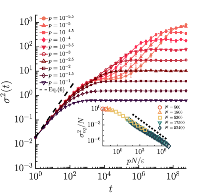
Figure 3: Wealth variance with different p𝑝p’s for ε=0.1𝜀0.1\varepsilon=0.1 on SF networks of N=887±13𝑁plus-or-minus88713N=887\pm 13, k¯=4.5¯𝑘4.5\overline{k}=4.5, and the degree exponent γ=2.5𝛾2.5\gamma=2.5, averaged over 100 realizations. Inset: data collapse of the rescaled wealth variance in the equilibrium state.

For sparse networks, the early- and late-time behaviors remain similar to those on the complete graphs as studied in Sec. III. See Fig. 3. However, in the intermediate-time regime, the wealth variance ceases to grow but remains fixed for a period and then resumes growth. These novel phases emerging on sparse networks are studied in this section, setting the ratio of RD transfers to be small.
Refer to caption
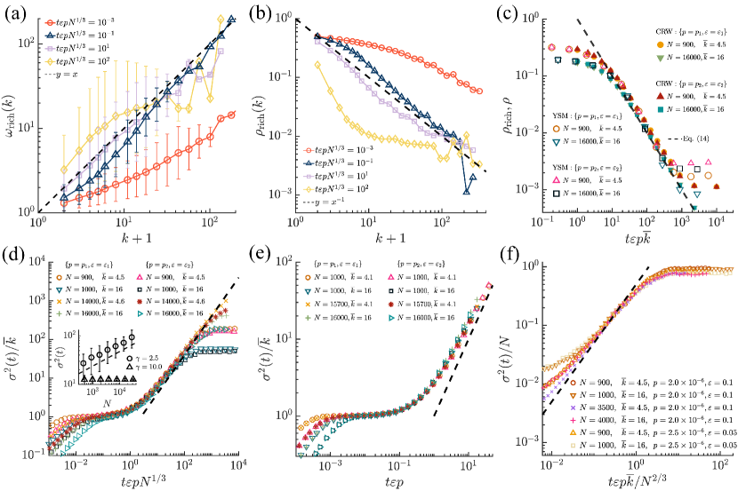
Figure 4: Scaling of wealth variance on SF networks. (a) Wealth of rich nodes versus degree plus one at different times for p=2.5×10⁶𝑝2.5superscript106p=2.5\times 10^{-6} and ε=0.05𝜀0.05\varepsilon=0.05 with N=27989±27𝑁plus-or-minus2798927N=27989\pm 27, k¯=4.5¯𝑘4.5\overline{k}=4.5, and γ=2.5𝛾2.5\gamma=2.5. (b) Plots of the probability ρrich(k)subscript𝜌rich𝑘\rho_{\rm rich}(k) of a node of degree k𝑘k to be rich. (c) Time-decay of the rich-node density ρrichsubscript𝜌rich\rho_{\rm rich} in the generalized YS model compared with the random-walker density ρ𝜌\rho in the CRW with (p1,ε1)=(2.0×106,0.1)subscript𝑝1subscript𝜀12.0superscript1060.1(p_{1},\varepsilon_{1})=(2.0\times 10^{-6},0.1) and (p2,ε2)=(2.5×106,0.05)subscript𝑝2subscript𝜀22.5superscript1060.05(p_{2},\varepsilon_{2})=(2.5\times 10^{-6},0.05) for γ=2.5𝛾2.5\gamma=2.5 and different N𝑁N’s and k¯¯𝑘\overline{k}’s. See Appendix B. The dashed line is Eq. (15). (d) Data collapse of the rescaled wealth variance as predicted in Eq. (16) with {(p1,ε1),(p2,ε2)}subscript𝑝1subscript𝜀1subscript𝑝2subscript𝜀2\{(p_{1},\varepsilon_{1}),(p_{2},\varepsilon_{2})\} as in (c) for γ=2.5𝛾2.5\gamma=2.5 and different N𝑁N’s and k¯¯𝑘\overline{k}’s. Inset: Wealth variance versus N𝑁N at fixed time t=1.25/εp𝑡1.25𝜀𝑝t=1.25/\varepsilon p with p=2.5×10⁶𝑝2.5superscript106p=2.5\times 10^{-6} and ε=0.05𝜀0.05\varepsilon=0.05 for two different γ𝛾\gamma’s. The dashed line has slope 1/3131\textfractionsolidus 3. (e) The same plots as in (e) for γ=10𝛾10\gamma=10. The dashed lines in (d) and (e) have slope 111. (f) Data collapse of the rescaled wealth variance exhibiting a crossover from the relaxation phase to the global condensate phase around teq=N2/3εpk¯subscript𝑡eqsuperscript𝑁23𝜀𝑝¯𝑘t_{\rm eq}={N^{2/3}\over\varepsilon p\overline{k}} with p<0.1p𝑝0.1subscript𝑝p<0.1p_{*} on the SF networks with γ=2.5𝛾2.5\gamma=2.5.

IV.1 Local condensate phase

In the local condensate phase for tlcttrelless-than-or-similar-tosubscript𝑡lc𝑡less-than-or-similar-tosubscript𝑡relt_{\rm lc}\lesssim t\lesssim t_{\rm rel}, the wealth variance is fixed, which is related to the sparse connection of the underlying network. Each rich node i𝑖i is found to have taken nearly all the wealth of its nearest neighbors, possessing ωi;richki+1similar-to-or-equalssubscript𝜔𝑖richsubscript𝑘𝑖1\omega_{i;{\rm rich}}\simeq k_{i}+1 including its own [Fig. 4(a)]. Hub nodes thus possess more as long as they are rich. Yet the probability of a node to be rich decreases with its degree as ρi;rich1ki+1similar-to-or-equalssubscript𝜌𝑖rich1subscript𝑘𝑖1\rho_{i;{\rm rich}}\simeq{1\over k_{i}+1} [Fig. 4(b)], for a node and its neighbor(s) are equally likely to be rich under the YS-mode transfer.

Introducing the wealth ωrich(k)subscript𝜔rich𝑘\omega_{\rm rich}(k) of a rich node of degree k𝑘k and the probability ρrich(k)subscript𝜌rich𝑘\rho_{\rm rich}(k) of a node of degree k𝑘k to be rich and approximating the wealth of a poor node to be zero, one can represent the wealth variance as

σ2kPdeg(k)[ρrich(k){ωrich(k)1}2+1ρrich(k)].similar-to-or-equalssuperscript𝜎2subscript𝑘subscript𝑃deg𝑘delimited-[]subscript𝜌rich𝑘superscriptsubscript𝜔rich𝑘121subscript𝜌rich𝑘\sigma^{2}\simeq\sum_{k}P_{\rm deg}(k)\left[\rho_{\rm rich}(k)\left\{\omega_{\rm rich}(k)-1\right\}^{2}+1-\rho_{\rm rich}(k)\right]. (13)

Using ρrich(k)1k+1similar-to-or-equalssubscript𝜌rich𝑘1𝑘1\rho_{\rm rich}(k)\simeq{1\over k+1} and ωrichk+1similar-to-or-equalssubscript𝜔rich𝑘1\omega_{\rm rich}\simeq k+1, we obtain

σ2k¯,similar-to-or-equalssuperscript𝜎2¯𝑘\sigma^{2}\simeq\overline{k}, (14)

as supported by Figs. 4(d) and (e). The onset time of local condensation tlck¯ε2similar-tosubscript𝑡lc¯𝑘superscript𝜀2t_{\rm lc}\sim\frac{\overline{k}}{\varepsilon^{2}}, at which Eq. (7) crossovers to Eq. (14), can be rationalized by considering that it takes time ε2superscript𝜀2\varepsilon^{-2} for a node to take the wealth of a neighbor by the YS-mode transfers, and it has k¯¯𝑘\overline{k} such neighbors on the average. Local condensation is terminated at trelsubscript𝑡relt_{\rm rel}, when the RD-mode transfers begin to redistribute significantly the wealth of the local rich nodes to their poor neighbors.

IV.2 Relaxation phase

On the time scale longer than trelsubscript𝑡relt_{\rm rel}, the RD transfers occur frequently enough to redistribute the locally-concentrated wealth to a neighboring node. Also one of the two wealths on neighboring nodes can absorb the other Lee . Such coalescence of wealth drives wealth to a single or a few nodes until the stationary state is reached, and we call this period the relaxation phase (treltteqless-than-or-similar-tosubscript𝑡rel𝑡less-than-or-similar-tosubscript𝑡eqt_{\rm rel}\lesssim t\lesssim t_{\rm eq}).

The wealth variance exhibits remarkable scaling behaviors [Fig. 4]. The dynamics of wealth in this phase can be understood by studying the coalescing random walk (CRW) on complex networks Catanzaro et al. (2005); Park (2020), which allows us to evaluate ρrich(k)subscript𝜌rich𝑘\rho_{\rm rich}(k) and ωrich(k)subscript𝜔rich𝑘\omega_{\rm rich}(k) and use them in Eq. (13) to obtain σ2(t)superscript𝜎2𝑡\sigma^{2}(t). In the CRW suited for our model, the following occurs for every link with rate λ𝜆\lambda: i) if the link is occupied by a walker (local wealth) at one end node and empty at the other end, the walker moves to the latter, ii) if both ends are occupied by walkers, they coalesce leaving one walker at either end, and iii) if both ends are empty, nothing happens over the link. One can show that the time-decrease of the walker density is proportional to the square of the density and obtain the solution ρ1λk¯tsimilar-to-or-equals𝜌1𝜆¯𝑘𝑡\rho\simeq{1\over\lambda\overline{k}t} as detailed in Appendix B. The jump rate λ𝜆\lambda is governed by the rate of RD transfers and given by λgYSεpsimilar-tosubscript𝜆gYS𝜀𝑝\lambda_{\rm gYS}\sim\varepsilon p. Therefore the fraction of rich nodes ρrichsubscript𝜌rich\rho_{\rm rich} in our model is given by

ρrich1εpk¯tsimilar-to-or-equalssubscript𝜌rich1𝜀𝑝¯𝑘𝑡\rho_{\rm rich}\simeq{1\over\varepsilon p\overline{k}t} (15)

for large t𝑡t. It is confirmed in simulations [Figs. 4(c)].

As random movement and coalescence of local wealth proceeds, the probability to be rich ρrich(k)subscript𝜌rich𝑘\rho_{\rm rich}(k) loses its dependence on degree k𝑘k [Fig. 4(b)]. The wealth of a node remains proportional to its degree [Fig. 4(a)] with the proportional coefficient increasing as the number of rich nodes decreases. Assuming ωrich(k)cksimilar-to-or-equalssubscript𝜔rich𝑘𝑐𝑘\omega_{\rm rich}(k)\simeq c\,k with c𝑐c a coefficient and ρrich(k)ρrichsimilar-to-or-equalssubscript𝜌rich𝑘subscript𝜌rich\rho_{\rm rich}(k)\simeq\rho_{\rm rich} in Eq. (15), one can use the unit-mean condition ω¯kPdeg(k)ρrich(k)ckρrichck¯=1similar-to-or-equals¯𝜔subscript𝑘subscript𝑃deg𝑘subscript𝜌rich𝑘𝑐𝑘similar-to-or-equalssubscript𝜌rich𝑐¯𝑘1\overline{\omega}\simeq\sum_{k}P_{\rm deg}(k)\rho_{\rm rich}(k)\,c\,k\simeq\rho_{\rm rich}\,c\,\overline{k}=1 to obtain c1ρrichk¯similar-to-or-equals𝑐1subscript𝜌rich¯𝑘c\simeq\frac{1}{\rho_{\rm rich}\overline{k}}. Using these results in Eq. (13), we find

σ2(t)ρrichc2k2¯{εpk¯N3γγ1tfor 2<γ<3,εpk¯tforγ>3,similar-to-or-equalssuperscript𝜎2𝑡subscript𝜌richsuperscript𝑐2¯superscript𝑘2similar-tocases𝜀𝑝¯𝑘superscript𝑁3𝛾𝛾1𝑡for2𝛾3𝜀𝑝¯𝑘𝑡for𝛾3\sigma^{2}(t)\simeq\rho_{\rm rich}\,c^{2}\,\overline{k^{2}}\sim\begin{cases}\varepsilon p\overline{k}N^{3-\gamma\over\gamma-1}t&{\rm for}\ 2<\gamma<3,\\ \varepsilon p\overline{k}t&{\rm for}\ \gamma>3,\end{cases} (16)

where we used kn¯k¯nmax{1,Nnγ+1γ1}similar-to¯superscript𝑘𝑛superscript¯𝑘𝑛1superscript𝑁𝑛𝛾1𝛾1{\overline{k^{n}}\over\overline{k}^{n}}\sim\max\{1,N^{n-\gamma+1\over\gamma-1}\} for the static-model SF networks Lee et al. (2004). The data collapses of the scaled plots for different ε,p,k¯𝜀𝑝¯𝑘\varepsilon,p,\overline{k} and N𝑁N in Fig. 4(d) and 4(e) confirm these scaling behaviors for 2<γ<32𝛾32<\gamma<3 and γ>3𝛾3\gamma>3, respectively.

V Multiple crossovers in wealth inequality

The results that we have obtained in the previous sections provide an overview of the multiple phases in the development of wealth inequality on sparse networks, depending on the ratio p𝑝p of the RD-mode transfers and the degree exponent γ𝛾\gamma. From Eqs. (7), (8), (14), and (16), we can expect the wealth variance to behave approximately as

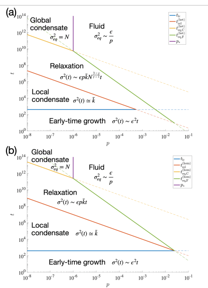
σ2(t){ε2tforttlc,k¯fortlcttrel,k¯εptmax{1,N3γγ1}fortreltteq,min{N,εp}fortteq.similar-tosuperscript𝜎2𝑡casessuperscript𝜀2𝑡much-less-thanfor𝑡subscript𝑡lc¯𝑘much-less-thanforsubscript𝑡lc𝑡much-less-thansubscript𝑡rel¯𝑘𝜀𝑝𝑡1superscript𝑁3𝛾𝛾1much-less-thanforsubscript𝑡rel𝑡much-less-thansubscript𝑡eq𝑁𝜀𝑝much-greater-thanfor𝑡subscript𝑡eq\sigma^{2}(t)\sim\begin{cases}\varepsilon^{2}t&{\rm for}\ t\ll t_{\rm lc},\\ \overline{k}&{\rm for}\ t_{\rm lc}\ll t\ll t_{\rm rel},\\ \overline{k}\varepsilon pt\max\{1,N^{3-\gamma\over\gamma-1}\}&{\rm for}\ t_{\rm rel}\ll t\ll t_{\rm eq},\\ \min\{N,{\varepsilon\over p}\}&{\rm for}\ t\gg t_{\rm eq}.\end{cases} (17)

The scaled plots in Fig.  4 (d) and (e) confirm the crossover around trelsubscript𝑡relt_{\rm rel} for ppmuch-less-than𝑝subscript𝑝p\ll p_{*}. The crossover around the equilibration time teqsubscript𝑡eqt_{\rm eq} is also shown in the data collapse of the scaled plots in Fig. 4(f).

The crossover time scales can be estimated by comparing the behaviors of σ2(t)superscript𝜎2𝑡\sigma^{2}(t) in adjacent time regimes in Eq. (17) and are given by

tlc=k¯ε2,subscript𝑡lc¯𝑘superscript𝜀2t_{\rm lc}={\overline{k}\over\varepsilon^{2}}, (18)
trelsubscript𝑡rel\displaystyle t_{\rm rel} =1εpmax{1,N3γγ1}absent1𝜀𝑝1superscript𝑁3𝛾𝛾1\displaystyle={1\over\varepsilon p\max\{1,N^{3-\gamma\over\gamma-1}\}} (19)
={trel(het)=1εpN3γγ1for 2<γ<3,teq(hom)=1εpforγ>3,absentcasessuperscriptsubscript𝑡relhet1𝜀𝑝superscript𝑁3𝛾𝛾1for2𝛾3superscriptsubscript𝑡eqhom1𝜀𝑝for𝛾3\displaystyle=\begin{cases}t_{\rm rel}^{\rm(het)}={1\over\varepsilon pN^{3-\gamma\over\gamma-1}}&{\rm for}\ 2<\gamma<3,\\ t_{\rm eq}^{\rm(hom)}={1\over\varepsilon p}&{\rm for}\ \gamma>3,\end{cases} (20)
teqsubscript𝑡eq\displaystyle t_{\rm eq} =min{N,εp}k¯εptmax{1,N3γγ1}absent𝑁𝜀𝑝¯𝑘𝜀𝑝𝑡1superscript𝑁3𝛾𝛾1\displaystyle={\min\{N,{\varepsilon\over p}\}\over\overline{k}\varepsilon pt\max\{1,N^{3-\gamma\over\gamma-1}\}} (21)
={teq,C(het)=N2(γ2)γ1εpk¯forpp, 2<γ<3,teq,F(het)=1p2k¯N3γγ1forpp, 2<γ<3,teq,C(hom)=Nεpk¯forpp,γ>3,teq,F(hom)=1p2k¯forpp,γ>3,absentcasessuperscriptsubscript𝑡eqChetsuperscript𝑁2𝛾2𝛾1𝜀𝑝¯𝑘formulae-sequencemuch-less-thanfor𝑝subscript𝑝2𝛾3superscriptsubscript𝑡eqFhet1superscript𝑝2¯𝑘superscript𝑁3𝛾𝛾1formulae-sequencemuch-greater-thanfor𝑝subscript𝑝2𝛾3superscriptsubscript𝑡eqChom𝑁𝜀𝑝¯𝑘formulae-sequencemuch-less-thanfor𝑝subscript𝑝𝛾3superscriptsubscript𝑡eqFhom1superscript𝑝2¯𝑘formulae-sequencemuch-greater-thanfor𝑝subscript𝑝𝛾3\displaystyle=\begin{cases}t_{\rm eq,C}^{\rm(het)}={N^{2(\gamma-2)\over\gamma-1}\over\varepsilon p\overline{k}}&{\rm for}\ p\ll p_{*},\ 2<\gamma<3,\\ t_{\rm eq,F}^{\rm(het)}={1\over p^{2}\overline{k}N^{3-\gamma\over\gamma-1}}&{\rm for}\ p\gg p_{*},\ 2<\gamma<3,\\ t_{\rm eq,C}^{\rm(hom)}={N\over\varepsilon p\overline{k}}&{\rm for}\ p\ll p_{*},\ \gamma>3,\\ t_{\rm eq,F}^{\rm(hom)}={1\over p^{2}\overline{k}}&{\rm for}\ p\gg p_{*},\ \gamma>3,\\ \end{cases} (22)

and the critical ratio psubscript𝑝p_{*} distinguishing the global condensate phase and fluid phase is given by pεNsubscript𝑝𝜀𝑁p_{*}\equiv{\varepsilon\over N}. We remark that on the complete graphs (k¯=N1¯𝑘𝑁1\overline{k}=N-1), the local condensate phase in Eq. (17) is identical to the global condensate phase σ2Nsimilar-to-or-equalssuperscript𝜎2𝑁\sigma^{2}\simeq N and therefore tlcsubscript𝑡lct_{\rm lc} in Eq. (18) should be considered as the equilibration time.
Refer to caption
Figure 5: Multiple phases of wealth inequality in the (p,t𝑝𝑡p,t) plane for the generalized YS model with ε=0.1𝜀0.1\varepsilon=0.1 on SF networks of N=105,k¯=4formulae-sequence𝑁superscript105¯𝑘4N=10^{5},\overline{k}=4 and (a) γ=2.5𝛾2.5\gamma=2.5 and (b) γ=10𝛾10\gamma=10. See Eq. (17). The phase boundaries are given by the crossover time scales in Eqs. (18), (20), and (22).

From Eqs. (17), (18), (20), and (22), we can obtain the diagram of different phases as in Fig. 5(a) and 5(b) for 2<γ<32𝛾32<\gamma<3 and γ>3𝛾3\gamma>3, respectively.

In these results, the influence of the network structure is significant: A large and heterogeneous network (small γ𝛾\gamma) facilitates wealth condensation by large wealth inequality and small trelsubscript𝑡relt_{\rm rel} and teqsubscript𝑡eqt_{\rm eq} as seen in Eqs. (17) to (22). Moreover, the correlation of wealth and node degree leads the wealth distribution to share the similar asymptotic behaviors with the degree distribution as will be detailed in the below. It is also remarkable that the RD transfers enable wealth inequality to resume growth but eventually decrease the stationary-state wealth inequality. The increase of the fraction ε𝜀\varepsilon not only speeds up the whole process, as shown in Eq. (6), but also increases stochasticity and thereby enhances the stationary-state wealth inequality as shown in Eq. (8).

Refer to caption
Figure 6: Inequality in the model and the real world. (a) Wealth distributions in the generalized YS model with p=2.5×10⁶,ε=0.05formulae-sequence𝑝2.5superscript106𝜀0.05p=2.5\times 10^{-6},\ \varepsilon=0.05 at different times on SF networks with N=16000,k¯=16formulae-sequence𝑁16000¯𝑘16N=16000,\overline{k}=16 and γ=2.5𝛾2.5\gamma=2.5. The solid and dashed lines are guide lines with different slopes. (b) Income distributions in several years between 1820 and 2020 obtained from the data-sets in Refs. Chancel and Piketty (2021) and  Chancel et al. (2022). Data have been rescaled so that the average is one, ω¯=1¯𝜔1\bar{\omega}=1. Inset: The power-law exponent α𝛼\alpha in P(ω)ωαsimilar-to𝑃𝜔superscript𝜔𝛼P(\omega)\sim\omega^{-\alpha} fitted to the data-sets for ω>10𝜔10\omega>10. (c) Wealth variance σ2superscript𝜎2\sigma^{2} and the Gini index of the rescaled income in the period 1820 to 2020 (filled points)  Chancel and Piketty (2021) and in the period 1980 to 2016 (open)  Chancel et al. (2022).

Finally, let us discuss the form of the wealth distribution on sparse networks. In the local condensate and the relaxation phase with small p𝑝p (ppmuch-less-than𝑝subscript𝑝p\ll p_{*}), there are a number of rich nodes as well as poor nodes. the poor nodes’ wealth, mostly much smaller than the average ωω¯=1much-less-than𝜔¯𝜔1\omega\ll\overline{\omega}=1, is found to be distributed by the power-law with exponent one, P(ω)ω1similar-to𝑃𝜔superscript𝜔1P(\omega)\sim\omega^{-1}, the same as the stationary-state distribution in Eq. (11). However, the distribution of rich nodes’ wealth is different, characterized by a larger power-law exponent than one as shown in Fig. 6(a). As we have shown in the main text, the origin lies in the correlation of the wealth of a rich node with its degree

ωrich(k)ck,similar-tosubscript𝜔rich𝑘𝑐𝑘\omega_{\rm rich}(k)\sim c\,k, (23)

where the coefficient c𝑐c is close to one in the local condensation phase (tlcttrelmuch-less-thansubscript𝑡lc𝑡much-less-thansubscript𝑡relt_{\rm lc}\ll t\ll t_{\rm rel}) and cεptsimilar-to-or-equals𝑐𝜀𝑝𝑡c\simeq\varepsilon\,p\,t in the relaxation phase (treltteqmuch-less-thansubscript𝑡rel𝑡much-less-thansubscript𝑡eqt_{\rm rel}\ll t\ll t_{\rm eq}) as shown in Sec. IV. Also, the probability of a node to be rich is given by

ρrich(k){1k+1fortlcttrel,ρrichfortreltteqsimilar-to-or-equalssubscript𝜌rich𝑘cases1𝑘1much-less-thanforsubscript𝑡lc𝑡much-less-thansubscript𝑡relsubscript𝜌richmuch-less-thanforsubscript𝑡rel𝑡much-less-thansubscript𝑡eq\rho_{\rm rich}(k)\simeq\begin{cases}{1\over k+1}&{\rm for}\ t_{\rm lc}\ll t\ll t_{\rm rel},\\ \rho_{\rm rich}&{\rm for}\ t_{\rm rel}\ll t\ll t_{\rm eq}\end{cases} (24)

with ρrichsubscript𝜌rich\rho_{\rm rich} given in Eq. (15). Therefore the wealth distribution P(ω)𝑃𝜔P(\omega) for large ω𝜔\omega is evaluated by using the degree distribution Pdeg(k)subscript𝑃deg𝑘P_{\rm deg}(k) as

P(ω)𝑃𝜔\displaystyle P(\omega) kPdeg(k)ρrich(k)δ(ωrich(k)ω)similar-toabsentsubscript𝑘subscript𝑃deg𝑘subscript𝜌rich𝑘𝛿subscript𝜔rich𝑘𝜔\displaystyle\sim\sum_{k}P_{\rm deg}(k)\rho_{\rm rich}(k)\delta(\omega_{\rm rich}(k)-\omega) (25)
Pdeg(kωc)ρrich(kωc)similar-toabsentsubscript𝑃degsimilar-to-or-equals𝑘𝜔𝑐subscript𝜌richsimilar-to-or-equals𝑘𝜔𝑐\displaystyle\sim P_{\rm deg}\left(k\simeq{\omega\over c}\right)\rho_{\rm rich}\left(k\simeq{\omega\over c}\right)
{ωγ1fortlcttrel,ωγfortreltteq.similar-toabsentcasessuperscript𝜔𝛾1much-less-thanforsubscript𝑡lc𝑡much-less-thansubscript𝑡relsuperscript𝜔𝛾much-less-thanforsubscript𝑡rel𝑡much-less-thansubscript𝑡eq\displaystyle\sim\begin{cases}\omega^{-\gamma-1}&{\rm for}\ t_{\rm lc}\ll t\ll t_{\rm rel},\\ \omega^{-\gamma}&{\rm for}\ t_{\rm rel}\ll t\ll t_{\rm eq}.\end{cases} (26)

This means that the power-law exponent of the wealth distribution P(ω)𝑃𝜔P(\omega) for large ω𝜔\omega may be between γ𝛾\gamma and γ+1𝛾1\gamma+1, probably changing from γ+1𝛾1\gamma+1 to γ𝛾\gamma with time, in the intermediate-time regime [Fig. 6(a)]. Approaching the stationary state, the number of rich nodes decreases [Eq. (15)] and therefore the fast-decaying right tail of P(ω)𝑃𝜔P(\omega) in Eq. (26) shrinks and eventually disappears in the stationary state.

The real-world income distributions, which are obtained by compiling the world income data in Refs. Chancel and Piketty (2021) and  Chancel et al. (2022) as described in Appendix C, decay slow for small income and then fast for large income with the latter characterized by a power-law of the exponent between 2 and 3. [Fig. 6(b)]. It is similar to the behavior of the wealth distribution in the intermediate-time regime; P(ω)ω1similar-to𝑃𝜔superscript𝜔1P(\omega)\sim\omega^{-1} for small ω𝜔\omega and Eq. (26) for large ω𝜔\omega. Different forms of the income distributions between the lower and upper class of the USA have been noted also in Ref. Ludwig and Yakovenko (2022). For comparison, we used the rescaled data so that the average income is equal to one. The income variance σ2superscript𝜎2\sigma^{2} is far from diverging with the population size, which would be the case with global wealth condensation; it increased from 20 to 50 in the period 1820 to 1900 and then decreased to less than 10 until around 1960, probably related to two world wars, and finally increased reaching σ220similar-to-or-equalssuperscript𝜎220\sigma^{2}\simeq 20 in 2020 [Fig. 6(c)].

VI Discussions

In this study, we have characterized the scaling properties of wealth inequality, represented by wealth variance, in both its dynamics and steady-state. In the process, we have identified the critical value for redistribution ratio which is inversely proportional to the population size. Furthermore, the evolution of wealth inequality on a sparsely-connected population undergoes multiple phases, revealing the effects of network structure: If heterogeneously connected, a large population progresses into an inequality at a greater rate than a small one, while if homogeneously connected, the population size does not affect the speed. This is direct consequence of the correlation between wealth and node degree. Our study thus demonstrates that the relevance of the network structure to the wealth distribution in the non-stationary state should be considered in analyzing the real-world wealth inequality.

The influence of the dimensionality of the underlying network on the speed of wealth condensation deserves investigation. The studied model is a minimal one, and can be extended with more data-sets of the real-world inequality.

Acknowledgements.
We thank Su-Chan Park for helpful discussion. This work was funded by KIAS Individual Grants (CG079902 (D.-S.L) and CG084501 (H.G.L)) at Korea Institute for Advanced Study. We are grateful to the Center for Advanced Computation in KIAS for providing computing resources.

Appendix A Boltzmann equation for p=0𝑝0p=0

When p𝑝p is small, in the long-time limit, the approximations that we take to obtain the left or right tail of the wealth distributions in Eqs. (9) and (10) are not working but one should refer to the Boltzmann equation Boghosian (2014)

P(ω,t)t=[P(ω,t)11+εP(ω1+ε,t)]𝑃𝜔𝑡𝑡delimited-[]𝑃𝜔𝑡11𝜀𝑃𝜔1𝜀𝑡\displaystyle\frac{\partial P(\omega,t)}{\partial t}=-\biggl{[}P(\omega,t)-\frac{1}{1+\varepsilon}P\Bigl{(}\frac{\omega}{1+\varepsilon},t\Bigr{)}\biggr{]}
[P(ω,t)11εP(ω1ε,t)]delimited-[]𝑃𝜔𝑡11𝜀𝑃𝜔1𝜀𝑡\displaystyle-\biggl{[}P(\omega,t)-\frac{1}{1-\varepsilon}P\Bigl{(}\frac{\omega}{1-\varepsilon},t\Bigr{)}\biggr{]}
+0ω1+ε𝑑ω[P(ωεω,t)11+εP(ω1+ε,t)]P(ω,t)superscriptsubscript0𝜔1𝜀differential-dsuperscript𝜔delimited-[]𝑃𝜔𝜀superscript𝜔𝑡11𝜀𝑃𝜔1𝜀𝑡𝑃superscript𝜔𝑡\displaystyle+\int_{0}^{\frac{\omega}{1+\varepsilon}}d\omega^{\prime}\biggl{[}P(\omega-\varepsilon\omega^{\prime},t)-\frac{1}{1+\varepsilon}P\Bigl{(}\frac{\omega}{1+\varepsilon},t\Bigr{)}\biggr{]}P(\omega^{\prime},t)
+0ω1ε𝑑ω[P(ω+εω,t)11εP(ω1ε,t)]P(ω,t)superscriptsubscript0𝜔1𝜀differential-dsuperscript𝜔delimited-[]𝑃𝜔𝜀superscript𝜔𝑡11𝜀𝑃𝜔1𝜀𝑡𝑃superscript𝜔𝑡\displaystyle+\int_{0}^{\frac{\omega}{1-\varepsilon}}d\omega^{\prime}\biggl{[}P(\omega+\varepsilon\omega^{\prime},t)-\frac{1}{1-\varepsilon}P\Bigl{(}\frac{\omega}{1-\varepsilon},t\Bigr{)}\biggr{]}P(\omega^{\prime},t) (27)

under the random-agent approximation. Then, one can find the following solution by direct substitution:

P(ω,t)=Cω(t+t0),𝑃𝜔𝑡𝐶𝜔𝑡subscript𝑡0\displaystyle P(\omega,t)=\frac{C}{\omega(t+t_{0})}, (28)

where t0subscript𝑡0t_{0} is a finite constant and C𝐶C is given by

C=1log(11ε2)1ϵ2𝐶111superscript𝜀2similar-to-or-equals1superscriptitalic-ϵ2\displaystyle C=\frac{1}{\log{\bigl{(}\frac{1}{1-\varepsilon^{2}}\bigr{)}}}\simeq{1\over\epsilon^{2}} (29)

with the last approximation valid for small ϵitalic-ϵ\epsilon.

Appendix B Density of random walkers in the CRW: Derivation of Eq. (15)

Following Catanzaro et al. (2005), we can see that the number of random walkers, ni=0subscript𝑛𝑖0n_{i}=0 or 111, on node i𝑖i at time t+dt𝑡𝑑𝑡t+dt in the CRW model is given by

ni(t+dt)=ni(t)η+(1ni(t))ξ,subscript𝑛𝑖𝑡𝑑𝑡subscript𝑛𝑖𝑡𝜂1subscript𝑛𝑖𝑡𝜉\displaystyle n_{i}(t+dt)=n_{i}(t)\eta+(1-n_{i}(t))\xi, (30)

where η𝜂\eta is 00 with probability λdtjaij(1nj)+λdtjaijnj=λdtki𝜆𝑑𝑡subscript𝑗subscript𝑎𝑖𝑗1subscript𝑛𝑗𝜆𝑑𝑡subscript𝑗subscript𝑎𝑖𝑗subscript𝑛𝑗𝜆𝑑𝑡subscript𝑘𝑖\lambda dt\sum_{j}a_{ij}(1-n_{j})+\lambda dt\sum_{j}a_{ij}n_{j}=\lambda\,dt\,k_{i} and 111 with probability 1λdtki1𝜆𝑑𝑡subscript𝑘𝑖1-\lambda\,dt\,k_{i}, and ξ𝜉\xi is 111 with probability λdtjaijnj𝜆𝑑𝑡subscript𝑗subscript𝑎𝑖𝑗subscript𝑛𝑗\lambda\,dt\sum_{j}a_{ij}n_{j} and 00 with probability 1λdtjaijnj1𝜆𝑑𝑡subscript𝑗subscript𝑎𝑖𝑗subscript𝑛𝑗1-\lambda\,dt\sum_{j}a_{ij}n_{j}. Here, η=0𝜂0\eta=0 represents the disappearance of the random-walker at node i𝑖i because of a jump to a nearest node (with probability λdtjaij(1nj)𝜆𝑑𝑡subscript𝑗subscript𝑎𝑖𝑗1subscript𝑛𝑗\lambda dt\sum_{j}a_{ij}(1-n_{j})), or coalescence to a neighbor node (with probability λdtjaijnj𝜆𝑑𝑡subscript𝑗subscript𝑎𝑖𝑗subscript𝑛𝑗\lambda dt\sum_{j}a_{ij}n_{j}). On the other hand, ξ=1𝜉1\xi=1 represents the arrival of a walker at node i𝑖i from a neighbor node (with probability λdtjaijnj𝜆𝑑𝑡subscript𝑗subscript𝑎𝑖𝑗subscript𝑛𝑗\lambda dt\sum_{j}a_{ij}n_{j}). Taking the ensemble average for a given ni(t)subscript𝑛𝑖𝑡n_{i}(t), we have

ni(t+dt)delimited-⟨⟩subscript𝑛𝑖𝑡𝑑𝑡\displaystyle\langle n_{i}(t+dt)\rangle =ni(t)(1λdtki)absentsubscript𝑛𝑖𝑡1𝜆𝑑𝑡subscript𝑘𝑖\displaystyle=n_{i}(t)\big{(}1-\lambda\,dt\,k_{i}\big{)}
+(1ni(t))λdtjaijnj(t),1subscript𝑛𝑖𝑡𝜆𝑑𝑡subscript𝑗subscript𝑎𝑖𝑗subscript𝑛𝑗𝑡\displaystyle+\big{(}1-n_{i}(t)\big{)}\lambda dt\sum_{j}a_{ij}n_{j}(t), (31)

which leads to

dρidt=λkiρi+λ(1ρi)jaijρj,𝑑subscript𝜌𝑖𝑑𝑡𝜆subscript𝑘𝑖subscript𝜌𝑖𝜆1subscript𝜌𝑖subscript𝑗subscript𝑎𝑖𝑗subscript𝜌𝑗\displaystyle\frac{d\rho_{i}}{dt}=-\lambda k_{i}\rho_{i}+\lambda\big{(}1-\rho_{i}\big{)}\sum_{j}a_{ij}\rho_{j}, (32)

where the density of random walker is denoted by ρi=nisubscript𝜌𝑖delimited-⟨⟩subscript𝑛𝑖\rho_{i}=\langle n_{i}\rangle and the independence of ρisubscript𝜌𝑖\rho_{i} and ρjsubscript𝜌𝑗\rho_{j} for ij𝑖𝑗i\neq j is assumed. Assuming that ρisubscript𝜌𝑖\rho_{i} at node i𝑖i is a function of its degree kisubscript𝑘𝑖k_{i} and equivalently ρi=ρjsubscript𝜌𝑖subscript𝜌𝑗\rho_{i}=\rho_{j} if ki=kjsubscript𝑘𝑖subscript𝑘𝑗k_{i}=k_{j}, we can rewrite Eq. (32) as

dρkdt=λkρk+λk(1ρk)kkPdeg(k)k¯ρk,𝑑subscript𝜌𝑘𝑑𝑡𝜆𝑘subscript𝜌𝑘𝜆𝑘1subscript𝜌𝑘subscriptsuperscript𝑘superscript𝑘subscript𝑃degsuperscript𝑘¯𝑘subscript𝜌superscript𝑘\displaystyle\frac{d\rho_{k}}{dt}=-\lambda k\rho_{k}+\lambda k\big{(}1-\rho_{k}\big{)}\sum_{k^{\prime}}\frac{k^{\prime}P_{\rm deg}(k^{\prime})}{\overline{k}}\rho_{k^{\prime}}, (33)

where ρk1Ni=1Nδki,kρisubscript𝜌𝑘1𝑁superscriptsubscript𝑖1𝑁subscript𝛿subscript𝑘𝑖𝑘subscript𝜌𝑖\rho_{k}\equiv\frac{1}{N}\sum_{i=1}^{N}\delta_{k_{i},k}\ \rho_{i} and Pdeg(k)subscript𝑃deg𝑘P_{\rm deg}(k) is the degree distribution of the underlying network. Note that ρ=kPdeg(k)ρk𝜌subscript𝑘subscript𝑃deg𝑘subscript𝜌𝑘\rho=\sum_{k}P_{\rm deg}(k)\rho_{k}. Let us also introduce ρ~kkPdeg(k)k¯ρk~𝜌subscript𝑘𝑘subscript𝑃deg𝑘¯𝑘subscript𝜌𝑘\tilde{\rho}\equiv\sum_{k}\frac{kP_{\rm deg}(k)}{\overline{k}}\rho_{k}. Multiplying Eq. (33) by Pdeg(k)subscript𝑃deg𝑘P_{\rm deg}(k) and summing over k𝑘k, we find

dρdt=λk¯ρ~+λk¯ρ~(1ρ~)=λk¯ρ~2.𝑑𝜌𝑑𝑡𝜆¯𝑘~𝜌𝜆¯𝑘~𝜌1~𝜌𝜆¯𝑘superscript~𝜌2\displaystyle\frac{d\rho}{dt}=-\lambda\overline{k}\tilde{\rho}+\lambda\overline{k}\tilde{\rho}\big{(}1-\tilde{\rho}\big{)}=-\lambda\overline{k}\tilde{\rho}^{2}. (34)

In the long-time limit, we expect dρkdt𝑑subscript𝜌𝑘𝑑𝑡\frac{d\rho_{k}}{dt} is much smaller than ρksubscript𝜌𝑘\rho_{k} or ρ~~𝜌\tilde{\rho} in Eq. (33), so we assume that the right-hand-side of Eq. (33) is zero, to obtain

ρkρ~1+ρ~,similar-to-or-equalssubscript𝜌𝑘~𝜌1~𝜌\displaystyle\rho_{k}\simeq\frac{\tilde{\rho}}{1+\tilde{\rho}}, (35)

which means that ρksubscript𝜌𝑘\rho_{k} is independent of k𝑘k. This also implies that

ρ=kPdeg(k)ρk=ρ~1+ρ~orρ~=ρ1ρ.formulae-sequence𝜌subscript𝑘subscript𝑃deg𝑘subscript𝜌𝑘~𝜌1~𝜌or~𝜌𝜌1𝜌\displaystyle\rho=\sum_{k}P_{\rm deg}(k)\rho_{k}=\frac{\tilde{\rho}}{1+\tilde{\rho}}\quad\text{or}\quad\tilde{\rho}=\frac{\rho}{1-\rho}. (36)

Inserting Eq. (36) into Eq. (34), we have

dρdt=λk¯(ρ1ρ)2λk¯ρ2,𝑑𝜌𝑑𝑡𝜆¯𝑘superscript𝜌1𝜌2similar-to-or-equals𝜆¯𝑘superscript𝜌2\displaystyle\frac{d\rho}{dt}=-\lambda\overline{k}\bigg{(}\frac{\rho}{1-\rho}\bigg{)}^{2}\simeq-\lambda\overline{k}\rho^{2}, (37)

where the last relation holds for ρ1much-less-than𝜌1\rho\ll 1 which will be valid in the long-time limit. Therefore, from Eq. (37), we have

ρ1λk¯t,similar-to-or-equals𝜌1𝜆¯𝑘𝑡\displaystyle\rho\simeq\frac{1}{\lambda\overline{k}t}, (38)

which gives ρrichρ1εpk¯tsimilar-tosubscript𝜌rich𝜌similar-to1𝜀𝑝¯𝑘𝑡\rho_{\rm rich}\sim\rho\sim\frac{1}{\varepsilon p\overline{k}t} with λgYS=εpsubscript𝜆𝑔𝑌𝑆𝜀𝑝\lambda_{gYS}=\varepsilon p as in Eq. (15) in the main text. It takes thop1εpsimilar-tosubscript𝑡hop1𝜀𝑝t_{\rm hop}\sim{1\over\varepsilon p} for the local wealth at a rich node i𝑖i to be fully redistributed to its poor neighbors and itself, which is understood by considering εpk¯ki(ωi1)thopωi1similar-to𝜀𝑝¯𝑘subscript𝑘𝑖subscript𝜔𝑖1subscript𝑡hopsubscript𝜔𝑖1{\varepsilon p\over\overline{k}}k_{i}(\omega_{i}-1)t_{\rm hop}\sim\omega_{i}-1 and essentially determines the rate λgYS1thopεpsimilar-to-or-equalssubscript𝜆gYS1subscript𝑡hopsimilar-to𝜀𝑝\lambda_{\rm gYS}\simeq{1\over t_{\rm hop}}\sim\varepsilon p of random hopping of local wealth.

Appendix C Income distribution in the real world in 1820 - 2020

We use two data-sets of the world income distribution, one in Ref. Chancel and Piketty (2021) covering a few selected years in the period 1820 to 2020 and the other in Ref. Chancel et al. (2022) providing annual data from 1980 to 2016. Both data-sets provide for each given year the average income W(x)𝑊𝑥W(x) of the people who belong to the top x𝑥x % of the whole population in the world regarding their income with x=0.01,0.1,1,10,50𝑥0.010.111050x=0.01,0.1,1,10,50, and 100100100. We can consider 6 distinct groups of people according to their income: bottom 50%, top 50% to top 10%, top 10% to top 1%, top 1% to top 0.1%, top 0.1% to top 0.01%, and the top 0.01%. The average incomes of the people in these 6 distinct groups and their portions are then given by

{W1=W(100)W(50),f1=0.5,W2=W(50)W(10),f2=0.4,W3=W(10)W(1),f3=0.09,W4=W(1)W(0.1),f4=0.009,W5=W(0.1)W(0.01),f5=0.0009,W6=W(0.01),f6=0.0001.casesformulae-sequencesubscript𝑊1𝑊100𝑊50subscript𝑓10.5otherwiseformulae-sequencesubscript𝑊2𝑊50𝑊10subscript𝑓20.4otherwiseformulae-sequencesubscript𝑊3𝑊10𝑊1subscript𝑓30.09otherwiseformulae-sequencesubscript𝑊4𝑊1𝑊0.1subscript𝑓40.009otherwiseformulae-sequencesubscript𝑊5𝑊0.1𝑊0.01subscript𝑓50.0009otherwiseformulae-sequencesubscript𝑊6𝑊0.01subscript𝑓60.0001otherwise\begin{cases}W_{1}=W(100)-W(50),\ f_{1}=0.5,\\ W_{2}=W(50)-W(10),\ f_{2}=0.4,\\ W_{3}=W(10)-W(1),\ f_{3}=0.09,\\ W_{4}=W(1)-W(0.1),\ f_{4}=0.009,\\ W_{5}=W(0.1)-W(0.01),\ f_{5}=0.0009,\\ W_{6}=W(0.01),\ f_{6}=0.0001.\end{cases} (39)

Notice that =16fi=1superscriptsubscript16subscript𝑓𝑖1\sum_{\ell=1}^{6}f_{i}=1. We can use these values to compute the mean wealth

W¯==16Wf.¯𝑊superscriptsubscript16subscript𝑊subscript𝑓\overline{W}=\sum_{\ell=1}^{6}W_{\ell}f_{\ell}. (40)

To compare the properties of these real-world incomes with the wealth considered in the main text, we consider the rescaled income

ω=WW¯subscript𝜔subscript𝑊¯𝑊\omega_{\ell}={W_{\ell}\over\overline{W}} (41)

for =1,2,3,4,5,6123456\ell=1,2,3,4,5,6. The income variance is then evaluated as

σ2==16ω2f1superscript𝜎2superscriptsubscript16superscriptsubscript𝜔2subscript𝑓1\sigma^{2}=\sum_{\ell=1}^{6}\omega_{\ell}^{2}f_{\ell}-1 (42)

and the (rescaled) income distribution P(ω)𝑃𝜔P(\omega) is obtained by

p(ω)=fΔω,𝑝subscript𝜔subscript𝑓Δsubscript𝜔p(\omega_{\ell})={f_{\ell}\over\Delta\omega_{\ell}}, (43)

where the bin sizes are evaluated as Δω=ωω+1ωω1Δsubscript𝜔subscript𝜔subscript𝜔1subscript𝜔subscript𝜔1\Delta\omega_{\ell}=\sqrt{\omega_{\ell}\omega_{\ell+1}}-\sqrt{\omega_{\ell}\omega_{\ell-1}} with ω0=ω12ω1ω2subscript𝜔0superscriptsubscript𝜔12subscript𝜔1subscript𝜔2\omega_{0}={\omega_{1}^{2}\over\sqrt{\omega_{1}\omega_{2}}} and ω7=ω62ω5ω6subscript𝜔7superscriptsubscript𝜔62subscript𝜔5subscript𝜔6\omega_{7}={\omega_{6}^{2}\over\sqrt{\omega_{5}\omega_{6}}}. We also compute the Gini index by

G=121=162=16|ω1ω2|f1f2,𝐺12superscriptsubscriptsubscript116superscriptsubscriptsubscript216subscript𝜔subscript1subscript𝜔subscript2subscript𝑓subscript1subscript𝑓subscript2G={1\over 2}\sum_{\ell_{1}=1}^{6}\sum_{\ell_{2}=1}^{6}|\omega_{\ell_{1}}-\omega_{\ell_{2}}|f_{\ell_{1}}f_{\ell_{2}}, (44)

where we used ω¯=1¯𝜔1\overline{\omega}=1. Note that the wealth variance σ2superscript𝜎2\sigma^{2} is represented by σ2=(1/2)1,2(ω1ω2)2f1f2superscript𝜎212subscriptsubscript1subscript2superscriptsubscript𝜔subscript1subscript𝜔subscript22subscript𝑓subscript1subscript𝑓subscript2\sigma^{2}=(1/2)\sum_{\ell_{1},\ell_{2}}(\omega_{\ell_{1}}-\omega_{\ell_{2}})^{2}f_{\ell_{1}}f_{\ell_{2}}.

References