Empirical Validation of a Class of
Ray-Based Fading Models

Abstract

As new wireless standards are developed, the use of higher operation frequencies comes in hand with new use cases and propagation effects that differ from the well-established state of the art. Numerous stochastic fading models have recently emerged under the umbrella of generalized fading conditions, to provide a fine-grain characterization of propagation channels in the mmWave and sub-THz bands. For the first time in literature, this work carries out an experimental validation of a class of such ray-based models, in a wide range of propagation conditions (anechoic, reverberation and indoor) at mmWave bands. We show that the independently fluctuating two-ray (IFTR) model has good capabilities to recreate rather dissimilar environments with high accuracy. We also put forth that the key limitations of the IFTR model arise in the presence of reduced diffuse propagation, and also due to a limited phase variability for the dominant specular components.

I Introduction

The advent and widespread deployment of the fifth generation (5G) of wireless technology has been key to improve the achievable data rates well-beyond tenths of Gbps, and also to reduce latency in one order of magnitude with respect to previous standards – now approaching to $1\text{\,}\mathrm{ms}$ [1]. One of the key enablers for such achievements is the use of higher frequency bands in the millimeter wave (mmWave) range. This trend is likely to continue as 5G evolves, and sixth generation (6G) is often envisioned to provide coverage in the sub-THz range for some use cases [2].

To properly modeling and describing propagation channels, different approaches can be taken to capture the true (and often intractable) nature of electromagnetic effects as signals traverse the wireless environment. Classically, channel modeling strategies have been categorized as empirical vs. analytical, and also as deterministic vs. stochastic [3]. Today, state-of-the-art channel models combine the key features from these approaches to improve accuracy. For instance, COST [4] and 3GPP-like [5] models combine empirical measurements (e.g. for path-loss exponents) with geometric modeling of the propagation environment, also incorporating some stochastic features to provide randomness inherent to wireless fading effects. These models often have hundreds of parameters that allow to recreate wireless propagation with high versatility, at the expense of a higher complexity and computational burden. Recently, ray-tracing approaches have been considered as an alternative to provide a realistic channel characterization in terms of a number of multipath components [6], at the price of an overwhelming mathematical complexity.

To circumvent the intricacy of these approaches, analytical stochastic channel models are of widespread use due to their comparatively reduced complexity, much fewer parameters, and mathematical tractability [7]. Rayleigh and Rician models are immensely popular in the wireless community, as the de facto standards to model small-scale fading in non line-of-sight (nLoS) and line-of-sight (LoS) cases, respectively. As new use cases promote the ubiquity of wireless devices, many new environments in sensor networks and industrial settings require the development of more advanced models, often referred to as generalized. For instance, the two-wave with diffuse power (TWDP) model [8] proposed by Durgin, Rappaport and de Wolf describes a multipath environment with two dominant constant-amplitude specular rays, plus an aggregate diffuse component. With only one parameter addition compared to the Rician case, the TWDP model has an increased capability to recreate not-so-common propagation conditions; these include bimodality and hyper-Rayleigh behaviour [9]. Subsequently, different generalizations and alternatives have been proposed in the literature: for instance, the fluctuating two-ray (FTR) model [10] allows that the two rays of the TWDP model fluctuate jointly or independently [11]. This philosophy is inherited from Abdi’s Rician-shadowed model [12], which also generalizes the Rician one. The $\kappa$-$\mu$ and the $\eta$-$\mu$ models proposed by Yacoub add additional flexibility to the Rician and Rayleigh models through the notion of multipath wave clusters. These were also later generalized by Paris’ $\kappa$-$\mu$ shadowed fading model [13].

Recently, it was shown that it is possible to bridge the gap between the models used for industry (e.g., 3GPP TR 38.901) and academia (e.g., ray based), by developing a MIMO channel model that calibrates the few parameters of the latter using the full 3GPP TR 38.901 channel model as a reference [14]. Clearly, the key to use any of the aforementioned statistical models for 5G performance evaluation in practical conditions is their empirical validation over a great variety of scenarios. One way to accomplish this is through measurement campaigns on a specific scenario; for instance, mobile radio channels over the sea at $5.9\text{\,}\mathrm{GHz}$ or vehicular channels during overtakes at $60\text{\,}\mathrm{GHz}$ exhibit TWDP behaviours [15, 16]. However, such campaigns are rather costly in terms of time and resources, and cannot be replicated in a controlled way. Another alternative is the use of laboratory chambers combining anechoic and reverberation features. These allow to recreate Rician-fading [17] or two-ray [18] environments, which can be exploited to emulate multiple-inputs multiple-outputs (MIMO) channels with such particular behaviour [19].

In this paper, we aim to empirically validate a class of ray-based stochastic fading models in a wide variety of scenarios. Specifically, we used our mixed anechoic/reverberation chamber facilities, together with indoor acquisition, to find a concordance between measurements and different propagation models in the frequency band between $24.25$ to $27.5\text{\,}\mathrm{GHz}$ (i.e., 3GPP n258 band), which belongs to the mmWave general classification [20]. For this purpose, we consider the independent fluctuating two-ray (IFTR) fading model recently proposed in [11], showing a remarkable goodness of fit in most scenarios. Interestingly, we identify that the widespread assumption of uniform phases for the two dominant specular components [8] does not hold in some scenarios with reduced multipath. We show that in those scenarios where this behavior is identified, a more general modeling for the phases [21] improves the fitting performance.

The remainder of the article is organized as follows. Section II summarizes the IFTR propagation model with the relevant physical and mathematical basis. Section III explains how the measures were acquired and how they are used for recreating new scenarios. Section IV shows and discuss the obtained results from fitting the scenarios with the propagation models. Finally, section V summarizes the key conclusions and the future lines derived from this work.

II Physical Channel Model

Let us consider a general formulation for the received radio signal over a wireless channel [22], given as a superposition of a number of waves

$$V_{r}=\sum_{n=1}^{M}A_{n}\exp\left({j\varphi_{n}}\right),$$ (1)

where $A_{n}$ and $\varphi_{n}$ denote their corresponding amplitudes and phases. Now, it is possible to reexpress (1) in the following way:

$$V_{r}=\sum_{n=1}^{N}A_{n}\exp\left({j\varphi_{n}}\right)+\underbrace{\sum_{m=1}^{P}A_{m}\exp\left({j\varphi_{m}}\right)}_{Z},$$ (2)

with $M=N+P$, so that $N$ now represents a group of dominant specular waves, while $P$ indicate a group of numerous and relatively weak diffusely propagating waves. For sufficiently large $P$, the central limit theorem (CLT) holds for the second term in (2), implying that $Z\triangleq\sum_{m=1}^{P}A_{m}\exp\left({j\varphi_{m}}\right)$ can be approximated as a complex Gaussian RV with zero-mean and variance $2\sigma^{2}$. For $N=2$, constant-amplitude $A_{n}$ and uniformly distributed phases $\varphi_{n}$, the TWDP model emerges [8]. In the sequel, and taking the TWDP model as a baseline reference, we consider the general case on which $A_{n}=V_{n}\sqrt{\xi_{n}}$ so that $V_{n}$ denotes the amplitude of each of these dominant specular components, whereas $\xi_{n}$ are unit-mean independent Gamma random variables characterizing amplitude fluctuations. This model, referred to as independently-fluctuating two-ray (IFTR) model, was recently formulated in [11], and is fully characterized by the following set of parameters:

$$K =\frac{V_{1}^{2}+V_{2}^{2}}{2\sigma^{2}}\in[0,\infty),$$ (3)

$$\Delta =\frac{2V_{1}V_{2}}{V_{1}^{2}+V_{2}^{2}}\in[0,1],$$ (4)

$$m_{n}\, \{n=1,2\}\in(0,\infty),$$ (5)

$$\Omega \triangleq{\rm E\{|V_{r}|^{2}\}}\in[0,\infty),$$ (6)

where $1/m_{n}$ denote the fading severity (i.e., the amount of fluctuation) for each of the specular components, $K$ is the Rician factor defined as the ratio between the average powers of the dominant specular waves and the diffuse components, and $\Delta$ captures the amplitude dissimilarity between the two dominant specular waves. Finally, the scale parameter $\Omega=V_{1}^{2}+V_{2}^{2}+2\sigma^{2}$ represents the average received power.

III Measurement Setup

The measurements consists in the channel response obtained for three different scenarios, namely: (semi)-anechoic and (semi)-reverberation chambers, and indoor. All of them has been analyzed in a great variety of Tx-Rx configurations in the mmWave frequency band from $24.25$ to $27.5\text{\,}\mathrm{GHz}$, sampled with $651$ points (that is, a $5\text{\,}\mathrm{MHz}$ step). A detailed description of the acquisition and the channel environments can be consulted in [23].

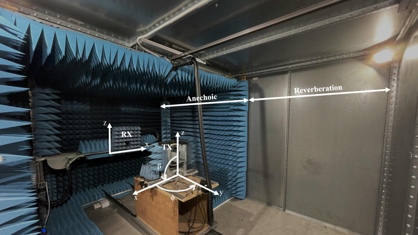
Figure 1: Panoramic of the half anechoic-reverberation chamber. The receiver antenna has movement in the XZ plane, but the transmitter only in $\phi$ and $\beta$ angles (named azimuth and roll respectively).

(a) $11\times 11$ receiver array in the XZ plane.

(b) Two-ray selection example.

Figure 2: Channel composing scheme in reverse path.

The first two scenarios were reproduced in a half anechoic-reverberation chamber whose dimensions are $$5$\times$3.5$\times$3.5$$ meters (see Fig. 1). The semi-anechoic side is completely covered with absorbents to suppress any possible reflection in order to receive exclusively the ray from the LoS path. In contrast, the semi-reverberation side is totally composed by metallic walls emerging a mutipath channel behaviour due to the multiple received reflected rays. The measured Tx-Rx configurations have been analogous for both cases, with a $160$ and $600\text{\,}\mathrm{cm}$ distance between antennas respectively. On the one hand, the receiver moves in $4\text{\,}\mathrm{cm}$ steps along the XZ plane, sweeping $11$ positions in each axis. The complete composition describes a $$40$\times$40$$ centimeters square centered on the transmitter-aligned position. On the other hand, the transmitter only modifies the pointing angle and the polarization with the azimuth and roll positions. In both cases, the transmitter sweeps three different values: $-30\mathrm{°}$, $0$ and $30\mathrm{°}$, taking the zero as the receiver-aligned in azimuth and roll coordinates (LoS path and no-depolarization losses).

The indoor setup is slightly different respect the chamber ones (an illustrative figure can be found in [23]). Transmitter was located inside the chamber, pointing to the door, while the receiver was placed outside, in the laboratory room. The movement for the latter has no changes, describing the $$40$\times$40$$ centimetres square. Nevertheless, the former modifies the azimuth variation adopting the following three angles: $-30\mathrm{°}$, $-15\mathrm{°}$ and $0$; keeping the previous for roll.

All the measurements were taken at the Smart and Wireless Applications and Techonologies (SWAT) research group facilities, located at the University of Granada (Spain). The acquisition was performed with a Vectorial Network Analyzer (VNA Rohde & Schwarz ZVA67), which is able to measure the scattering parameters operating up to $67\text{\,}\mathrm{GHz}$. The receiver and transmitter antennas were standardized gain horns fed with a WR-34 waveguide-to-coaxial transition (Flann K-band antenna model: #21240-20). Finally, the transmit power was set to $10\text{\,}\mathrm{d}\mathrm{B}\mathrm{m}$ in the VNA.

The described setup results in $1089$ point-to-point measurements per environment where, in most of cases, only one ray would be relevant. For the anechoic case, all reflected rays are deeply attenuated by construction. Furthermore, at this frequency band (up to $27.5\text{\,}\mathrm{GHz}$) scattering effects have low relevance. In order to recreate a two-ray propagation channels, linear combinations are computed adding the contributions of two original measurements. The main condition to give them a real physical meaning is that receiver or transmitter position has to be locked in the same position. This leads to classify the possible configurations in two groups: ”direct” and ”reverse” paths respectively (see Fig. 2). The former represents channels where the two-rays differs in polarization and pointing, with the same Tx-Rx physical path. For the latter, however, the physical path differs while keeping the transmitter polarization and pointing unchanged.

The application of the exposed method results in a large amount of possible combinations. Because of that, only a reduced selection of $142$ configurations for each measured scenario have been selected to work with, searching for significance differences between them. For a fair comparison, all of them correspond to the same Tx-Rx configurations in anechoic, reverberation and indoor scenarios. Conductive to illustrate this fact, two animations have been included in the supplementary material for the reader. Fig. 3 shows the great diversity of channel probability density functions, where rician-like and bimodal behaviours are found, these latter especially in the anechoic case. The last ones implies there are two common values of received amplitude, one associated to the mode of the distribution and the other to the next local maxima. Additionally, PDF shapes with higher complexity such as trimodal and beyond are sometimes observed in the selected set.

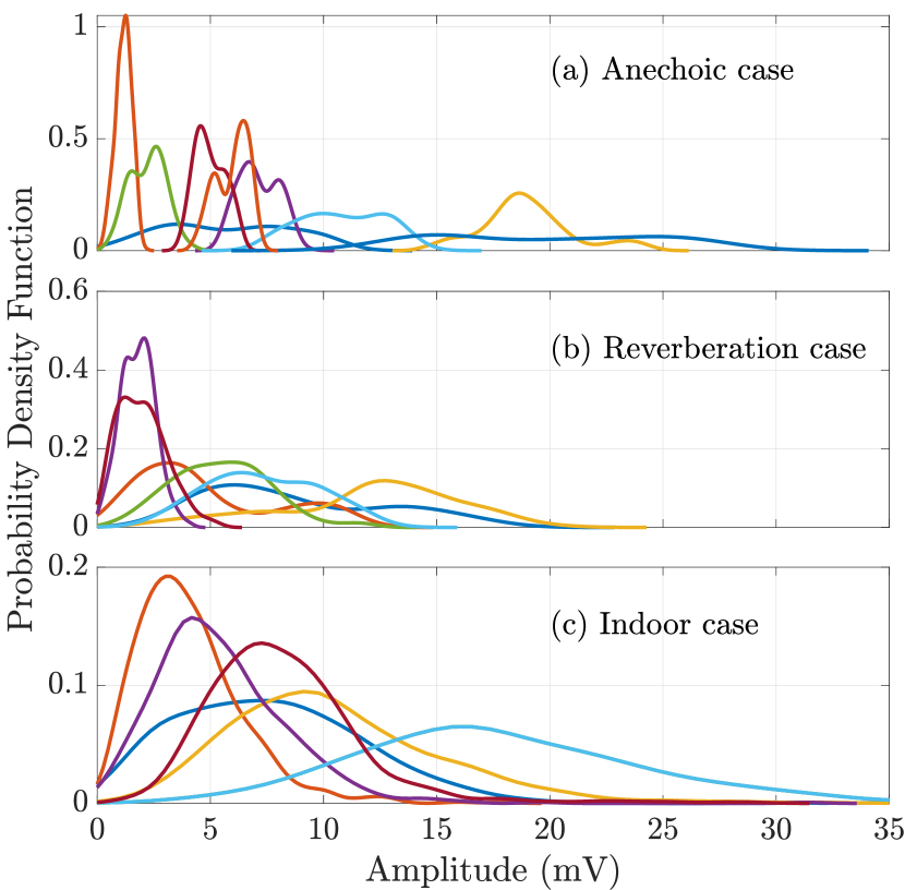
Figure 3: Channel configurations diversity per scenario.

IV Empirical Validation and Analysis

IV-A IFTR channel fitting

Once the Tx-Rx configurations have been chosen, a fitting between the empirical PDFs and the IFTR theoretical one is carried out. A common way is the use of optimization numerical algorithms such as gradient descent (GDA) or genetic algorithms (GA) in order to minimize an objective function, corresponding to a given error metric to be minimized. In this work, a multi-objective optimization problem has been established for finding the Pareto front for the following set of error metrics as targets:

• Mean Squared Error:

  $$\mathrm{MSE}\triangleq\frac{1}{N}\sum_{i=1}^{N}(f_{\rm exp}(x_{i})-f_{\rm mod}(x_{i}))^{2}.$$ (7)

• Root Mean Squared Error:

  $$\mathrm{RMSE}\triangleq\sqrt{\frac{1}{N}\sum_{i=1}^{N}(f_{\rm exp}(x_{i})-f_{\rm mod}(x_{i}))^{2}}.$$ (8)

• Mean Absolute Error:

  $$\mathrm{MAE}\triangleq\frac{1}{N}\sum_{i=1}^{N}|f_{\rm exp}(x_{i})-f_{\rm mod}(x_{i})|.$$ (9)

• Modified Kolmogorov-Smirnov statistic:

  $$\mathrm{KS}\triangleq\max_{x_{i}}|f_{\rm exp}(x_{i})-f_{\rm mod}(x_{i})|.$$ (10)

The use of multiple objective functions aims to find differences between the fitting results when minimizing each of the error metrics.

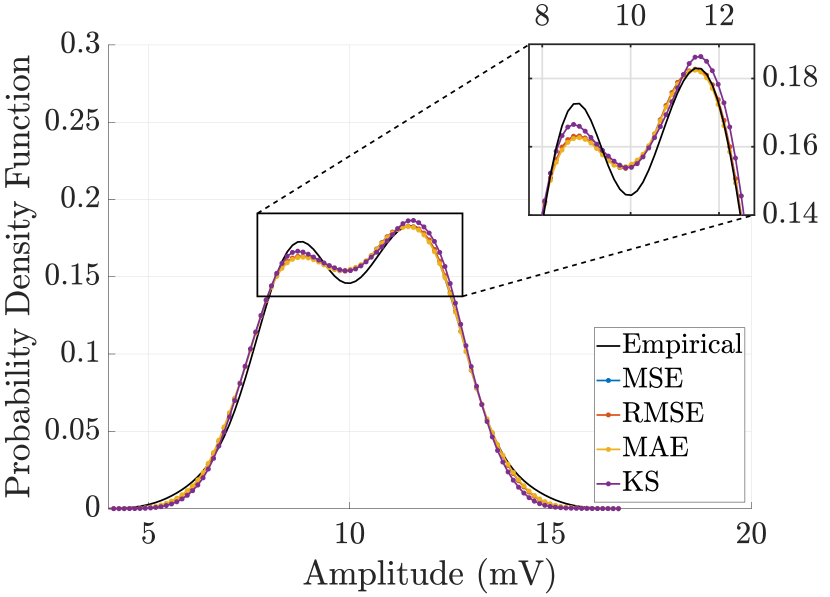
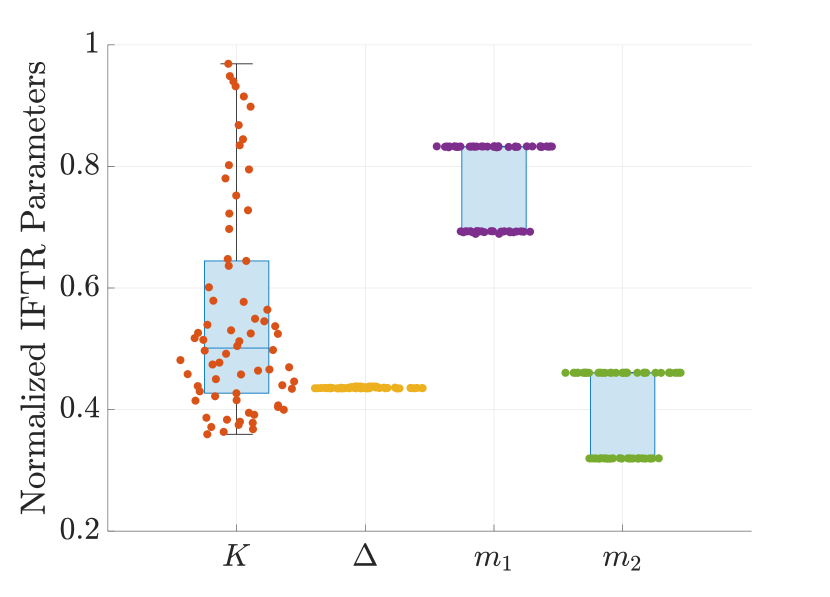
Figure 4: Comparison between the IFTR PDFs associated to the minimum of each error metric (anechoic case A).

Figure 5: IFTR parameters of the complete Pareto front in anechoic conf. A. Values are normalized respect the upper limit established for the GA search.

TABLE I: IFTR parameters for each minimum error metric solution of the Pareto front in anechoic cofiguration A.

	Min. Error Metric Solutions (Conf. A)
Parameter	MSE	RMSE	MAE	KS
Error	$16.56$	$4.07$	$2.96$	$8.18$
$K$ [$\mathrm{dB}$]	$28.6$	$28.6$	$27.2$	$27.3$
$\Delta$	$0.44$	$0.44$	$0.44$	$0.44$
$(m_{1},m_{2})$	$($35$,$16$)$	$($35$,$16$)$	$($35$,$16$)$	$($42$,$23$)$

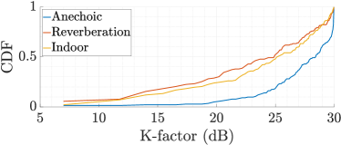
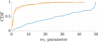
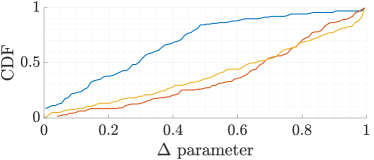
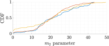
Figure 6: Comparison of the optimal IFTR parameters CDFs for the three analysed environments.

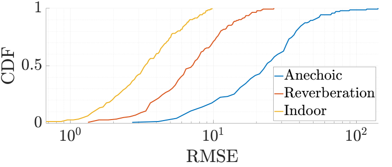
Figure 7: RMSE metric CDFs for the three scenarios.

To solve the optimization problem, the chosen algorithm is the NSGA-II [25], an elitist GA designed for working with real numbers. A population size of $200$ and generations number of $400$ has been set, with $30\text{\,}\mathrm{dB}$ and $50$ as upper limits for both $K$ and $\{m_{1},m_{2}\}$ IFTR parameters respectively. The elite count (number of individuals guaranteed to survive to the next generation) is a $5$% of the population. Finally, as stop criterion, a number of $100$ generations without significance changes in the solutions is taken as a convergence signal.

After the GA execution, a Pareto front set is obtained for each configuration per scenario. Fig. 5 shows a comparison for an arbitrary selected anechoic scenario named A between the particular solutions that minimize each metric (see Table I). It is clear that solutions produces similar curves shape, even if the Pareto point is different. In fact, a common behaviour is the presence of two well-defined solutions as in Fig. 5, where the GA has found two local minima for $m_{1}$ and $m_{2}$. On the other hand, an unique value for $\Delta$ meanwhile the factor $K$ varies over a higher range.

For the purpose of choosing a particular Pareto point $P$ in the form $(K,\Delta,m_{1},m_{2})$ as final fitting result, a weighed normalized error metric $\varepsilon_{n}$ is computed as follows:

$$\varepsilon_{n}(P)\triangleq\left.\frac{\mathrm{MSE}_{n}+\mathrm{RMSE}_{n}+\mathrm{MAE}_{n}+\mathrm{KS}_{n}}{4}\right|_{P},$$ (11)

where $[\>\cdot\>]_{n}$ refers to the normalization of each error metric respect its maximum from the complete Pareto front. Then, the chosen solution is the particular point $\hat{P}$ that minimizes this $\varepsilon_{n}$ function:

$$\hat{P}=\min_{P}\varepsilon_{n}(P).$$ (12)

In Fig. 6 the CDFs of the optimal IFTR parameters for each scenario are represented. The most remarkable fact is the contrast between anechoic and multipath cases, with a noticeable different trend in the curves. The Rician-like $K$ factor takes higher values due to the absence of diffuse power, whereas the $\Delta$ parameter concentrates in lower values because of the lack of reflections in LoS (the two rays are notably different). The $m_{1}$ parameter shows that the fluctuation of the first ray is less pronounced in the anechoic case, which is explained by the no presence of strong reflections. However, the second ray fluctuates in a similar way for the three analysed scenarios as the $m_{2}$ curves are quite close. The values for the multipath cases are larger than in the first, which implies that the fitting model assumes the second ray (with a lower amplitude) to be less fluctuating.

TABLE II: Fitting results for the example configurations in each scenario.

		Configuration
Parameter	Scenario	A	B	C	D	E	F
$K$ [$\mathrm{dB}$]	Anechoic	$29.3$	$27.8$	$29.9$	$25.0$	$29.9$	$30.0$
	Reverberation	$25.8$	$27.3$	$29.4$	$29.8$	$22.7$	$26.3$
	Indoor	$22.8$	$25.6$	$29.9$	$27.1$	$29.9$	$20.6$
$\Delta$	Anechoic	$0.44$	$0.09$	$0.23$	$1.00$	$0.45$	$0.21$
	Reverberation	$0.09$	$0.80$	$0.49$	$0.73$	$0.33$	$0.52$
	Indoor	$0.58$	$0.24$	$0.02$	$1.00$	$0.54$	$0.99$
$(m_{1},m_{2})$	Anechoic	$($35$,$16$)$	$($27$,$13$)$	$($50$,$35$)$	$($11$,$22$)$	$($36$,$12$)$	$($50$,$14$)$
	Reverberation	$($12$,$19$)$	$($1$,$18$)$	$($1$,$33$)$	$($0.60$,$0.39$)$	$($15$,$27$)$	$($3$,$32$)$
	Indoor	$($0.69$,$19$)$	$($0.93$,$22$)$	$($0.46$,$15$)$	$($5$,$38$)$	$($1$,$25$)$	$($2$,$25$)$
$\rm RMSE$	Anechoic	$4.10$	$16.46$	$26.51$	$33.48$	$9.10$	$16.64$
	Reverberation	$4.00$	$9.71$	$4.22$	$10.41$	$3.10$	$2.46$
	Indoor	$4.30$	$3.52$	$8.86$	$4.24$	$1.10$	$3.29$

To compare the fitting accuracy between the analyzed scenarios, the RMSE metric associated to each solution is studied. Fig. 7 shows the CDFs in the three analyzed scenarios. We see that the indoor case is associated to the lowest error, which confirms that the multipath richness is beneficial for fitting to the IFTR model. Conversely, the largest RMSE corresponds to the anechoic case; we will later evaluate the reasons for such behavior, which are linked to some of the underlying assumptions for the IFTR model.

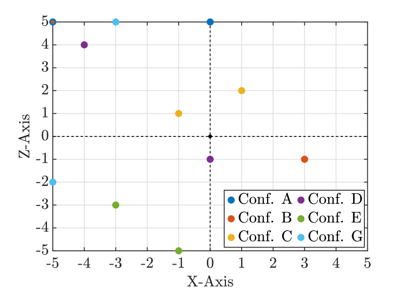
Figure 8: Configurations selected to be shown as PDF fitting examples. For chamber scenarios: A, E and F correspond to angles $\{\phi,\beta\}=\{$$,$$\}$, B to $\{\phi,\beta\}=\{$$,$$\}$; and C and D to $\{\phi,\beta\}=\{$$,$$\}$. Indoor scenario changes azimuth variation to $-15\mathrm{°}$, $-30\mathrm{°}$ and $0\mathrm{°}$ respectively.

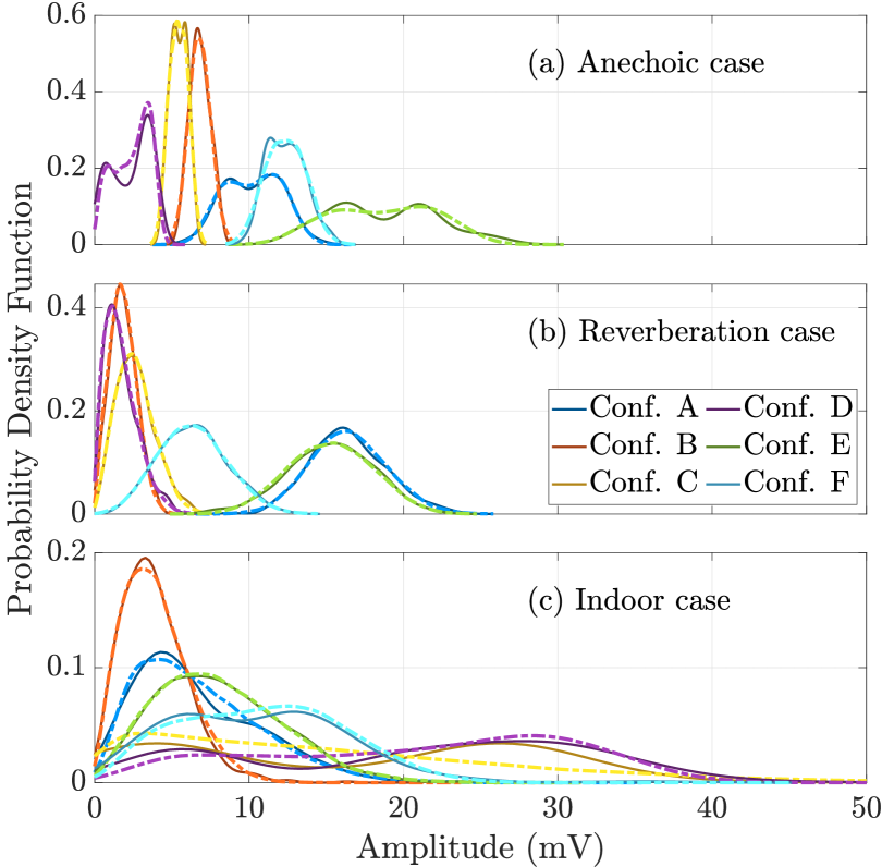
Figure 9: PDF fitting examples for different configurations. Dashed and solid lines represent, respectively, empirical and IFTR optimal solution.

In order to exemplify some particular PDF fittings, six sample configurations (A, B, C, D, E, and F; see Fig. 8) results shall be found in Fig. 9. This figure visually shows the good accuracy of the model for describing the channel over the three scenarios (numerical results can be consulted in Table II). In fact, Rician/Rayleigh-like channels usually associated to reverberation scenarios are also improved when using the IFTR model. As supplementary material for the reader, an additional animation showing PDF solutions for each configuration with the complete pareto front and the error metrics is included.

IV-B Anechoic environment

As mentioned previously, anechoic scenarios are associated to higher fitting error than multipath ones. Although most of the configurations can be described with a high accuracy, there exists a certain percentage of fitted configurations with an unsatisfactory goodness of fit (GoF). After a thorough analysis, the key aspect that justifies this behavior is the lack of phase diversity, which has two main implications: on the one hand, it causes that the CLT assumption for the diffuse component is not met; on the other hand, it affects the assumption of uniformly distributed phases for the dominant specular components, as the travelled path by the two-rays is insufficient to produce all phases between $-\pi$ and $\pi$.

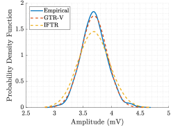
(a) Configuration G.

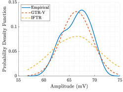
(b) Configuration H.

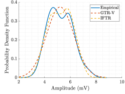
(c) Configuration I.

Figure 10: Comparison between fitted IFTR and GTR-V PDFs for particular anechoic configurations.

The implications of a non-uniform phase distribution have been discussed in [21], where the TWDP model was modified to account for this particular situation. The resulting model, termed as GTR-V, has the following PDF for the received amplitude:

$$f_{\rm GTR-V}(r)=\int_{-\pi}^{\pi}f_{\rm rice}(r;K[1+\Delta\cos(\alpha)])f_{\alpha}(\alpha)\mathrm{d}\alpha,$$ (13)

where $f_{\rm rice}()$ is the well-known Rician distribution with a factor $K_{r}=K[1+\Delta\cos(\alpha)]$, given by

$$f_{\rm rice}(r;K_{r})=\frac{r}{\sigma^{2}}\exp\left(-\frac{r^{2}}{2\sigma^{2}}-K_{r}\right)I_{0}\left(\frac{r}{\sigma}\sqrt{2K_{r}}\right),$$ (14)

with $I_{0}()$ being the modified Bessel function of the first class and order zero, whereas $f_{\alpha}()$ represents the phase difference distribution. In the GTR-V channel model, this corresponds to a von Mises PDF [26]:

$$f_{\alpha}(\alpha;\kappa,\phi)=\frac{\exp(\kappa\cos(\alpha-\phi))}{2\pi I_{0}(\kappa)}\>\>\forall\>\>\alpha\in[-\pi,\pi],$$ (15)

where $\phi\in\mathbb{R}$ represents the mean of the distribution and $\kappa\geq 0$ is inversely related to its variance.

While it is indeed possible to generalize the IFTR model to incorporate the effect of a non-uniform phase distribution following the rationale in [21], this would imply that the resulting model would have two additional parameters, incurring in additional complexity when it comes to fitting. Instead, we will use the GTR-V model even though it has no fluctuation on the two dominant specular components; in practice, this is equivalent to assuming a sufficiently large value of $m_{1}$ and $m_{2}$ in the IFTR model (see Fig. 6). Therefore, the use of this alternative model is well-justified for the sake of simplicity. After analyzing the distribution of the phase difference between the dominant specular components in the relevant anechoic configurations, a small sub-set with a von Mises like PDF has been selected (named confs. G, H and I).

The fitting process for the GTR-V model has been carried out as a two-step optimization problem. First, the empirical phase difference distribution is modelled as a von Mises distribution, finding the two parameters $\phi$ and $\kappa$ that provide the best fit for the phase distribution alone. After finding these parameters, a second optimization is performed in an analogous way as for IFTR finding the best pair $\{K,\Delta\}$ of GTR-V model applying GA search.

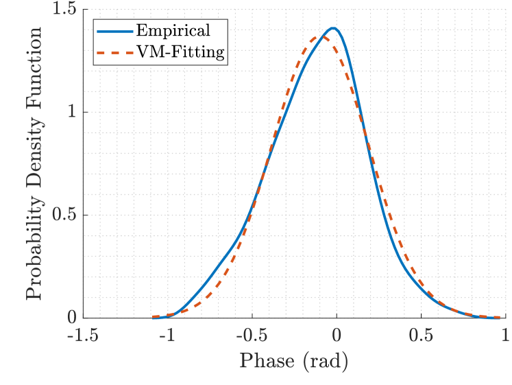
Figure 11: Phase difference fitting with von Mises distribution for the anechoic configuration G.

TABLE III: Comparison between IFTR and GTR-V modelling.

		Anechoic configuration
Model	Parameter	G	H	I
IFTR	$K$ [$\mathrm{dB}$]	$30.0$	$30.0$	$25.1$
	$\Delta$	$2.7\text{\times}{10}^{-3}$	$0.7\text{\times}{10}^{-3}$	$0.40$
	$(m_{1},m_{2})$	$($50$,$32$)$	$($50$,$5$)$	$($31$,$13$)$
2-5	$\mathrm{RMSE}$	$142.38$	$28.17$	$17.58$
GTR-V	$K$ [$\mathrm{dB}$]	$19.8$	$23.8$	$10.6$
	$\Delta$	$0.45$	$2.6\text{\times}{10}^{-4}$	$0.11$
	$\phi$	$-0.10$	$0.08$	$-0.10$
	$\kappa$	$12.04$	$638.94$	$1.23$
2-5	$\mathrm{MSE_{VM}}$	$2.9\text{\times}{10}^{-3}$	$0.19$	$6.2\text{\times}{10}^{-4}$
	$\mathrm{RMSE}$	$37.66$	$10.04$	$28.66$

Fig. 11 shows the fitting of the phase difference distribution with a von Mises PDF for configuration G. After the first step of the optimization, the resulting parameters $\kappa$ and $\phi$ yield an MSE of $0.0029$, which implies an excellent GoF. The next step is find the optimal parameters for the GTR-V model by the use of GA. The obtained results for the configurations G, H and I are summarized in Table III, and a visual comparison for the PDFs can be found in Fig. 10. For configurations G and H, we see that the GTR-V model has a better capability to improve the fitting. The effect of a non-uniform phase distribution is translated into an effective reduction of the variance, and it can visually confirmed that the GTR-V model achieves this. However, we see that the fitting is not improved when the PDF is bimodal – see configuration I in Fig. 10. We see that the original ability of the TWDP model to capture bimodality is affected when including the effect of non-uniform phases in the GTR-V model.

IV-C Multipath environments

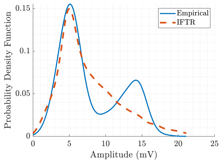
(a) Configuration J (reverberation).

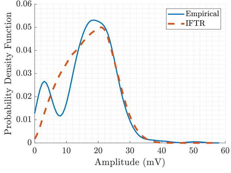
(b) Configuration K (indoor).

Figure 12: PDFs empirical and fitted for extreme bimodality behaviours.

Multipath environments, as Fig. 7 shows, have lower RMSE compared to the anechoic ones. This implies that most of the configurations has been described correctly with the IFTR model, as confirmed in Fig. 9. However, we have identified some cases on which the fitting to IFTR fails, which are explained next. Specifically, we have identified that in the event of sharp bimodal behaviors, that we refer henceforth as extreme bimodality, the ability of the IFTR model to capture such bimodality is not enough. This is exemplified in Fig. 12 for configurations J and K. In these situations, the model tries to fit the dominant peak but masking the secondary one. Numerical results can be consulted in Table IV.

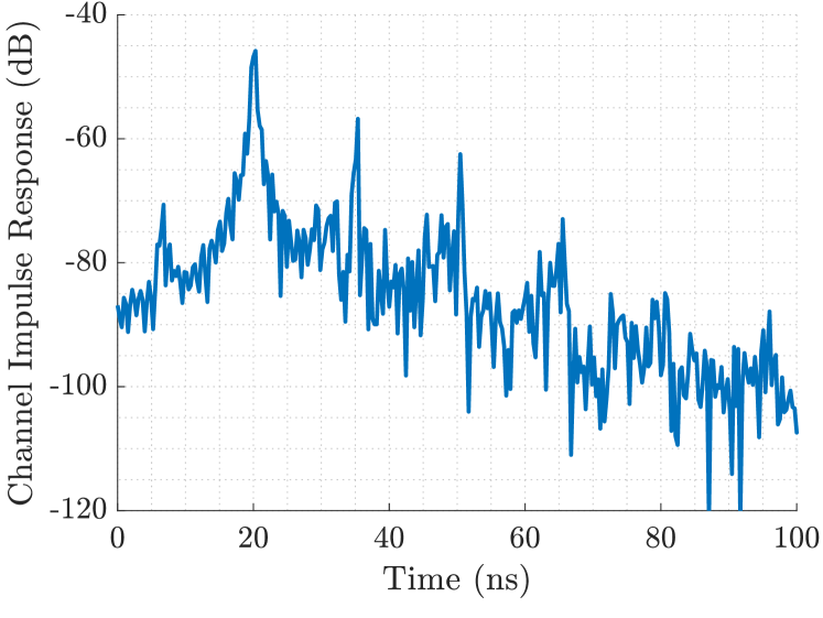
(a) Configuration J (reverberation).

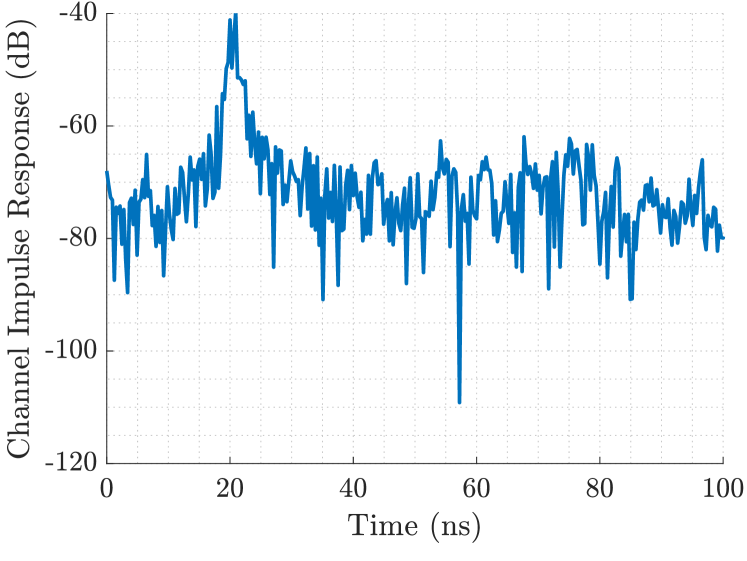
(b) Configuration K (indoor).

Figure 13: CIR for multipath configurations with extreme bimodality behaviours.

TABLE IV: IFTR solutions for multipath configurations with extreme bimodality behaviours.

	Multipath configuration
Parameter	J (reverberation)	K (indoor)
$K$ [$\mathrm{dB}$]	$28.9$	$28.2$
$\Delta$	$0.92$	$0.87$
$(m_{1},m_{2})$	$($0.45$,$30$)$	$($3$,$31$)$
1-3 $\mathrm{RMSE}$	$18.27$	$6.33$

One way to determine the origin of this particular behaviour is to analyze the CIR of the path. Fig. 13 shows the estimation of the channel time response for configurations J and K. The former reveals that there are more than two rays arriving at the antenna, situation not covered by the IFTR model. The presence of several rays may cause a high variation in the received amplitude, which can result in a high imbalance between the modal values. The latter, however, presents two dominant rays but with a high proximity in time. Hence, its interaction may not be described independently as the IFTR model predicts. Even though the consideration of additional rays can be usually encompassed by integrating these into the diffuse component [24], this is not the case when the overall number of rays is reduced, multipath propagation is limited, and there is a lack of phase richness in the propagation environment.

V Conclusions

We conducted an empirical validation of the independently-fluctuating two-ray fading model, covering a wide range of scenarios in the frequency band n258 (from $24.25\text{\,}\mathrm{GHz}$ to $27.5\text{\,}\mathrm{GHz}$). We confirmed that the IFTR model is highly versatile, and is able to recreate rather dissimilar propagation conditions including anechoic, reverberation and indoor scenarios. Besides, the four shape parameters that characterize the model have a solid physical meaning, which agrees with the expected properties of each analyzed channel.

We also observed some relevant effects that put forth the limitations of the IFTR model: (i) the assumption of uniform phases for the dominant specular components does not always hold, especially when there is a lack of phase richness. This is the case in scenarios with a reduced multipath, and is likely to become a dominant effect as we move up in frequency; (ii) the IFTR model is not able to capture extreme bimodal behaviors observed in some of the measurements. This can be caused by the combination of a number of effects, such as the presence of additional rays (due to spurious reflections), the absence of rich multipath propagation, and the interaction between dominant specular components. In this regard, the development of physically-motivated models that capture these behaviours deserves special attention, together with additional empirical validations at higher frequencies.

Appendix

The supplementary material is available at the IEEE DataPort repository: https://dx.doi.org/10.21227/hzw9-6q21. It consists in three different animations, where two of them present the channel diversity along the computed combinations and the other one the obtained solutions for the IFTR fitting. The former present multitude of configurations with a representative scheme, the associated PDF of received amplitude for each scenario and the phase difference PDF. The latter shows the obtained solutions for the Pareto front, the distribution of the IFTR parameters and the RMSE metric, the phase PDF and the associated configuration scheme.

References

- [1] T. S. Rappaport, Y. Xing, G. R. MacCartney, A. F. Molisch, E. Mellios, and J. Zhang, “Overview of Millimeter Wave Communications for Fifth-Generation (5G) Wireless Networks—With a Focus on Propagation Models,” IEEE Trans. Antennas Propag., vol. 65, pp. 6213–6230, dec 2017.
- [2] M. Polese, J. M. Jornet, T. Melodia, and M. Zorzi, “Toward End-to-End, Full-Stack 6G Terahertz Networks,” IEEE Commun. Mag., vol. 58, no. 11, pp. 48–54, 2020.
- [3] D. W. Matolak, “Channel Modeling for Vehicle-To-Vehicle Communications,” IEEE Commun. Mag., vol. 46, no. 5, pp. 76–83, 2008.
- [4] COST Action 231 (Project) and European Commission. DGXIII ”Telecommunications, Information Market, and Exploitation of Research.”, Digital Mobile Radio Towards Future Generation Systems: Final Report. European Commission, Directorate-General Telecommunications, Information Society, Information Market, and Exploitation of Research, 1999.
- [5] 3rd Generation Partnership Project, “5G; Study on channel model for frequencies from 0.5 to 100 GHz (3GPP TR 38.901 version 17.0.0 Release 17),” tech. rep., European Telecommunications Standards Institute, Apr. 2022.
- [6] M. Lecci, P. Testolina, M. Polese, M. Giordani, and M. Zorzi, “Accuracy Versus Complexity for mmWave Ray-Tracing: A Full Stack Perspective,” IEEE Trans. Wireless Commun., vol. 20, no. 12, pp. 7826–7841, 2021.
- [7] M. K. Simon and M.-S. Alouini, Digital Communication over Fading Channels (Wiley Series in Telecommunications and Signal Processing). Wiley-IEEE Press, 2004.
- [8] G. Durgin, T. Rappaport, and D. de Wolf, “New analytical models and probability density functions for fading in wireless communications,” IEEE Trans. Commun., vol. 50, pp. 1005–1015, jun 2002.
- [9] J. Frolik, “On appropriate models for characterizing hyper-Rayleigh fading,” IEEE Trans. Wireless Commun., vol. 7, no. 12, pp. 5202–5207, 2008.
- [10] J. M. Romero-Jerez, F. J. Lopez-Martinez, J. F. Paris, and A. J. Goldsmith, “The Fluctuating Two-Ray Fading Model: Statistical Characterization and Performance Analysis,” IEEE Trans. Wireless Commun., vol. 16, pp. 4420–4432, jul 2017.
- [11] M. Olyaee, J. A. Cortes, F. J. Lopez-Martinez, J. F. Paris, and J. M. Romero-Jerez, “The Fluctuating Two-Ray Fading Model with Independent Specular Components,” IEEE Trans. Veh. Technol., vol. 72, no. 5, pp. 5533–5545, 2023.
- [12] A. Abdi, W. Lau, M. Alouini, and M. Kaveh, “A new simple model for land mobile satellite channels: first- and second-order statistics,” IEEE Trans. Wirel. Commun., vol. 2, pp. 519–528, may 2003.
- [13] J. F. Paris, “Statistical characterization of - shadowed fading,” IEEE Trans. Veh. Technol., vol. 63, pp. 518–526, Feb 2014.
- [14] M. Pagin, S. Lagén, B. Bojovic, M. Polese, and M. Zorzi, “Improving the Efficiency of MIMO Simulations in ns-3,” in Proceedings of the 2023 Workshop on ns-3, pp. 1–9, 2023.
- [15] E. Zochmann, M. Hofer, M. Lerch, S. Pratschner, L. Bernado, J. Blumenstein, S. Caban, S. Sangodoyin, H. Groll, T. Zemen, A. Prokes, M. Rupp, A. F. Molisch, and C. F. Mecklenbrauker, “Position-Specific Statistics of 60 GHz Vehicular Channels During Overtaking,” IEEE Access, vol. 7, pp. 14216–14232, 2019.
- [16] K. Yang, N. Zhou, A. F. Molisch, T. Roste, E. Eide, T. Ekman, J. Yu, F. Li, and W. Chen, “Propagation measurements of mobile radio channel over sea at 5.9 GHz,” in 2018 16th International Conference on Intelligent Transportation Systems Telecommunications (ITST), IEEE, oct 2018.
- [17] C. Holloway, D. Hill, J. Ladbury, P. Wilson, G. Koepke, and J. Coder, “On the Use of Reverberation Chambers to Simulate a Rician Radio Environment for the Testing of Wireless Devices,” IEEE Trans. Antennas Propag., vol. 54, pp. 3167–3177, nov 2006.
- [18] J. Frolik, T. M. Weller, S. DiStasi, and J. Cooper, “A Compact Reverberation Chamber for Hyper-Rayleigh Channel Emulation,” IEEE Trans. Antennas Propag., vol. 57, no. 12, pp. 3962–3968, 2009.
- [19] J. D. Sanchez-Heredia, J. F. Valenzuela-Valdes, A. M. Martinez-Gonzalez, and D. A. Sanchez-Hernandez, “Emulation of MIMO Rician-Fading Environments With Mode-Stirred Reverberation Chambers,” IEEE Trans. Antennas Propag., vol. 59, pp. 654–660, feb 2011.
- [20] 3rd Generation Partnership Project, “5G; NR; User Equipment (UE) radio transmission and reception; Part 2: Range 2 Standalone (3GPP TS 38.101-2 version 17.5.0 Release 17),” tech. rep., European Telecommunications Standards Institute, Apr. 2022.
- [21] M. Rao, F. J. Lopez-Martinez, M.-S. Alouini, and A. Goldsmith, “MGF Approach to the Analysis of Generalized Two-Ray Fading Models,” IEEE Trans. Wirel. Commun., pp. 1–1, 2015.
- [22] G. D. Durgin, Theory of stochastic local area channel modeling for wireless communications. PhD thesis, Virginia Polytechnic Institute and State University, 2000.
- [23] A. Ramirez-Arroyo, L. Garcia, A. Alex-Amor, and J. F. Valenzuela-Valdes, “Artificial Intelligence and Dimensionality Reduction: Tools for Approaching Future Communications,” IEEE Open J. Commun. Soc., vol. 3, pp. 475–492, 2022.
- [24] J. M. Romero-Jerez, F. J. Lopez-Martinez, J. P. Peña-Martín, and A. Abdi, “Stochastic Fading Channel Models With Multiple Dominant Specular Components,” IEEE Trans. Veh. Technol., vol. 71, no. 3, pp. 2229–2239, 2022.
- [25] K. Deb and D. Kalyanmoy, Multi-Objective Optimization Using Evolutionary Algorithms. Wiley, 2001.
- [26] V. M. R., “Uber die ’ganzzahligkeit’ der atomgewicht und verwandte fragen,” Physikal. Z., vol. 19, pp. 490–500, 1918.