Directionality of nuclear recoils in a liquid argon time projection chamber

Abstract

The direct search for dark matter in the form of weakly interacting massive particles (WIMP) is performed by detecting nuclear recoils (NR) produced in a target material from the WIMP elastic scattering. A promising experimental strategy for direct dark matter search employs argon dual-phase time projection chambers (TPC). One of the advantages of the TPC is the capability to detect both the scintillation and charge signals produced by NRs. Furthermore, the existence of a drift electric field in the TPC breaks the rotational symmetry: the angle between the drift field and the momentum of the recoiling nucleus can potentially affect the charge recombination probability in liquid argon and then the relative balance between the two signal channels. This fact could make the detector sensitive to the directionality of the WIMP-induced signal, enabling unmistakable annual and daily modulation signatures for future searches aiming for discovery. The Recoil Directionality (ReD) experiment was designed to probe for such directional sensitivity. The TPC of ReD was irradiated with neutrons at the INFN Laboratori Nazionali del Sud, and data were taken with $72\text{\,}\mathrm{keV}\text{/}$ NRs of known recoil directions. The direction-dependent liquid argon charge recombination model by Cataudella et al. was adopted and a likelihood statistical analysis was performed, which gave no indications of significant dependence of the detector response to the recoil direction. The aspect ratio $R$ of the initial ionization cloud is estimated to be $1.037\pm 0.027$ and the upper limit is $R<1.072$ with $90\text{\,}\mathrm{\char 37\relax}\text{/}$ confidence level.

1 Introduction

A range of evidences from astronomy and cosmology Ade:2016bk ; Rubin:1999hb ; Clowe:2006hr ; Covone:2009ji ; Malaney:1993ep indicates that a substantial fraction of the Universe is made of non-baryonic dark matter, whose nature is still unknown. Weakly interacting massive particles (WIMPs), a common candidate, are actively searched for by many experiments worldwide using different technologies Schumann:2019eaa ; Cebrian:2022brv ; Roszkowski:2017nbc . The expected signal of those direct dark matter experiments is the nuclear recoil (NR) induced by the WIMP elastic scattering, having energy up to a few tens of $\mathrm{keV}\text{/}$. To improve sensitivity, it is crucial to strongly suppress any NR generating contamination, until the “neutrino fog” is reached, i.e. the irreducible background from coherent elastic neutrino-nucleus scattering.

While evidence of WIMPs could be claimed based on an excess of NRs with respect to the expected background, a convincing discovery requires the observation of the effect in many target materials and the consistency with strong and unmistakable dark matter signatures. The motion of the Solar system relative to the galactic dark matter halo creates an apparent WIMP flux through terrestrial detectors coming from the direction opposite to the Earth’s velocity vector, i.e. approximately from the Cygnus constellation. Furthermore, the motion of the Earth around the Sun generates annual modulations in the flux strength and direction. These signatures can be detected in the angular distribution of NRs produced by WIMP elastic scattering in a terrestrial detector, which would be an unmistakable “smoking gun” for dark matter, as none of the known backgrounds, including coherent neutrino scattering, can mimic it.

Directional sensitivity would hence be a crucial asset for future direct dark matter search experiments, especially when claiming a signal. Even in a detector with moderate angular resolution ($\sim$20\text{\,}\mathrm{\SIUnitSymbolDegree}\text{/}$$) for NRs, a few hundreds of events would be sufficient to reject the hypothesis of isotropic incident flux at $3\sigma$ level Cadeddu:2017ebu . A number of R&D programs is currently in progress for directional direct dark matter search Ahlen:2009ev ; Hochberg:2016ntt ; Battat:2016pap ; Vahsen:2020pzb ; Belli:2022jqq .

One of the most promising current approaches for the direct search of WIMPs is based on argon dual-phase Time Projection Chambers (TPC). It offers extremely low background thanks to the efficient rejection of the electron recoil (ER) background provided by pulse shape discrimination (PSD) Amaudruz:2016dq and the use of low-radioactivity argon from underground sources Galbiati:2007xz ; Aalseth:2020nwt . Based on the successful experience of the DarkSide-50 experiment Agnes:2015gu ; Agnes:2015ftt ; Agnes:2018ves at the Gran Sasso Laboratory (LNGS) of INFN and of the DEAP-3600 experiment DEAP-3600:2017uua ; DEAP:2019yzn at SNOLAB, the Global Argon Dark Matter Collaboration (GADMC) is pursuing a multi-staged experimental program aiming to improve the sensitivity down to the “neutrino fog” Aalseth:2017fik . Currently, GADMC is preparing for the DarkSide-20k experiment Aalseth:2017fik which features a 50 tonne underground argon dual-phase TPC with Silicon Photomultiplier readout.

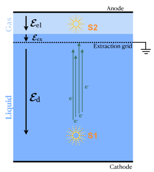
Figure 1: Conceptual sketch of the working principle of a double-phase argon TPC, illustrating a typical event with both a primary scintillation signal (S1) and a secondary electroluminescence signal (S2). The electric field in three different regions of the TPC is indicated here as the drift field ($\mathcal{E}_{d}$), extraction field ($\mathcal{E}_{ex}$) and electroluminescence field ($\mathcal{E}_{el}$). Figure from Ref. Agnes:2021zyq .

The working principle of an argon dual-phase TPC is depicted in Fig. 1. The TPC contains a volume of liquid argon (LAr) with a thin layer of gaseous argon, the gas pocket, on the top. The elastic scattering of a hypothetical WIMP particle with an Ar nucleus in the TPC would originate a NR of kinetic energy ranging from $\sim 20$ to $\sim 100$ keV, which ionizes the medium along its trajectory. The energy deposition of an ionizing particle which travels in the liquid volume produces excitation and ionization, giving rise to excited argon dimers (Ar${}_{2}^{*}$) and to electron-ion pairs. The de-excitation of Ar${}_{2}^{*}$ dimers, some of which are produced by electron-ion recombination, emits scintillation light, which produces the S1 signal. The residual unrecombined ionization electrons are swept away from the interaction site and drifted towards the liquid-gas interface by an appropriate electric field, the drift field $\mathcal{E}_{d}$. They are extracted to the gas phase and accelerated by intense fields, the extraction field $\mathcal{E}_{ex}$​ and the electrolumiscence field $\mathcal{E}_{el}$, respectively. Accelerated electrons in the gas phase emit light by electroluminescence Aalseth:2020zdm ; Buzulutskov:2020xhd , which is the S2 signal. The S1 and S2 signals are separated by the time interval corresponding to the electron drift time from the interaction site to the gas phase. The S2 signal intensity is proportional to the number of extracted electrons. The recombination of electrons with ions produces Ar dimers at the expense of free charge and therefore affects the balance between the intensity of S1 and S2 signals.

A dual-phase TPC could potentially offer a directional sensitivity for the events featuring long straight ionization tracks, thanks to the mechanism of columnar recombination Jaffe:1913gs ; Birks:1951boa ; Cataudella:2017kcf . When the track is nearly parallel to $\mathcal{E}_{d}$, electrons pass through the electron-ion column from the track itself and have a higher probability to meet an Ar ion and recombine, compared to a perpendicular track. Events with tracks parallel to $\mathcal{E}_{d}$ are therefore expected to have an enhanced S1 and a reduced S2. According to Refs. Nygren:2013fy ; Cao:2015ks , the directional dependence occurs only if the charge cloud around the ionization track is anisotropic, namely when the ionizing track is longer than the Onsager radius $r_{O}$, the distance between an ion and a free electron for which the electrostatic potential energy equals the thermal kinetic energy of the electron. As $r_{O}=e^{2}/(6\pi\epsilon_{0}\epsilon_{r}k_{B}T)$ is about $80\text{\,}\mathrm{nm}\text{/}$ in LAr ($T=87$ K, $\epsilon_{r}=1.5$), argon ions with kinetic energy above $\sim$40\text{\,}\mathrm{keV}\text{/}$$ have a range longer than $r_{O}$ srim . Therefore, an argon dual-phase TPC could potentially be direction-sensitive in the energy range of interest for WIMP searches. However, calculations and simulations Wojcik:2003ja ; Wojcik:2016gy show that the mean thermalization distance of electrons in LAr is about $2.6\text{\,}\mathrm{\SIUnitSymbolMicro m}\text{/}$, which is much longer than the Onsager radius and of the range of WIMP-induced recoils. As recombination mostly takes place when electrons are fully thermalized, the directional sensitivity could hence be diluted by electron diffusion during thermalization.

The SCENE Collaboration has provided a hint of directional sensitivity in the S1 signal for NRs of about $60\text{\,}\mathrm{keV}\text{/}$ Cao:2015ks , and specifically a difference of about 7% on S1 for NRs parallel and perpendicular to the drift field, at $\mathcal{E}_{d}$=193 V/cm.

The breakthrough that the directional sensitivity of an argon TPC would offer in the framework of direct dark matter searches motivated the Recoil Directionality (ReD) experiment, as a part of the program of the GADMC. ReD Agnes:2021zyq has been designed and performed with the goals to scrutinize the hint by SCENE, by testing a directional effect with a size as reported by SCENE, and additionally to provide new experimental data to improve the understanding of recombination and thermalization of electrons in LAr.

To this aim, a miniaturized argon dual-phase TPC was irradiated with neutrons at INFN, Laboratori Nazionali del Sud, to produce NRs at a variety of angles with respect to the TPC drift field. The kinetic energy of NRs is around $70\text{\,}\mathrm{keV}\text{/}$, which falls in the range of interest of WIMP search in Ar and corresponds to an ion range larger than the Onsager radius. This work is organized as follows: Sect. 2 discusses the models to describe the response of an argon dual-phase TPC to NRs of the energy relevant for dark matter searches, including the potential directional dependence. The experimental layout of ReD and the description of the individual detectors are given in Sect. 3 and 4, respectively. The data treatment, including reconstruction calibration, event selection, and the subsequent statistical analysis for directional sensitivity are presented in Sect. 5 and 6. The results and their potential impact are discussed in Sect. 7, followed by the summary of conclusions in Sect. 8.

2 The response of Ar to nuclear recoils

WIMPs deposit energy in LAr through elastic scattering on Ar nuclei. The subsequent energy loss of the NR involves nuclear stopping, ionization, charge recombination, and scintillation. Through the series of physical processes, the total energy deposited in the TPC is eventually divided into the detectable photons (S1) and electrons (S2), and the undetectable phonons (heat).

Directional modulation of charge recombination is expected when the spatial charge distribution of ionization is anisotropic. Conventional NR charge recombination models often assume an isotropic charge distribution. For example, the commonly-used Thomas-Imel model Thomas:1987ek ; Szydagis:2011tk assumes that charges are uniformly distributed in a cubic box of size $a$; the only free parameter for a given detector material is the initial charge $Q_{0}$. The probability of charge surviving recombination under the electric drift field $\mathcal{E}_{d}$ is

$$p(a,Q_{0})=\frac{\mathcal{E}_{d}}{\xi(a,Q_{0})}\ln\left(1+\frac{\xi(a,Q_{0})}{\mathcal{E}_{d}}\right),$$ (1)

where

$$\xi(a,Q_{0})=\frac{\alpha Q_{0}}{4a^{2}\mu_{-}};$$ (2)

$\alpha$ is the Langevin recombination coefficient Langevin1903 ; Bubon:2016hc , which depends on the carrier mobilities ($\mu_{-}$ and $\mu_{+}$ for electrons and ions, respectively) and on the dielectric constant as

$$\alpha=\frac{(\mu_{-}+\mu_{+})}{\epsilon_{0}\epsilon_{r}}.$$ (3)

In order to introduce the directionality, the electron distribution after thermalization needs to be included in the model. One approach is to use the Jaffé model Jaffe:1913gs ; Birks:1951boa , commonly referred to as the columnar recombination model, where the charge distribution is modeled by a column with radius $b$, length $l$, and angle $\theta$ between its axis $\hat{r}_{0}$ and the drift field $\mathcal{E}_{d}$. The Jaffé model is commonly adopted for the straight tracks from minimum ionizing particles. Since NR tracks are more localized, a more general and flexible parameterization of the charge distribution $q_{0}(\vec{r})$ has been proposed by Cataudella et al. Cataudella:2017kcf , which consists of a three dimensional Gaussian with an elliptical profile

$$q_{0}(\vec{r})=\frac{Q_{0}}{(2\pi)^{3/2}R\sigma^{3}}\exp{\left(-\left(\frac{\vec{r}\cdot\hat{r}_{0}}{R\sigma}\right)^{2}-\left(\frac{\vec{r}\times\hat{r}_{0}}{\sigma}\right)^{2}\right)},$$ (4)

where $\sigma$ characterizes the size of the distribution, $\hat{r}_{0}$ is the direction vector of the long axis, and $R$ is the aspect ratio between the long and short axes. The probability of charge surviving recombination is calculated in Ref. Cataudella:2017kcf as

$$p(R,\theta,Q_{0})=-\frac{\mathcal{E}_{d}f(R,\theta)}{\xi_{m}}\mathrm{Li}_{2}\left(-\frac{\xi_{m}}{\mathcal{E}_{d}f(R,\theta)}\right),$$ (5)

where

$$\xi_{m}=\frac{\alpha Q_{0}}{2\pi\sigma^{2}\mu_{-}}$$ (6)

is the generalization of the Thomas-Imel parameter $\xi$ of Eq. 2 and $\mathrm{Li}_{2}$ is the second order polylogarithm function. The term $f(R,\theta)$ captures the directionality dependence and it has the functional form

$$f(R,\theta)=\sqrt{R^{2}\sin^{2}\theta+\cos^{2}\theta},$$ (7)

being $\theta$ the angle between $\hat{r}_{0}$ and $\mathcal{E}_{d}$. When $R=1$, $f(R,\theta)=1$, so directionality vanishes and Eq. 5 reduces to the Thomas-Imel model.

Since directionality effects do not occur before recombination, well-established models are used here to describe the S1 and S2 yields, that for NRs also depend on nuclear and electronic quenching. Following the Lindhard model Lindhard:1963vo ; Bezrukov:2010qa , the nuclear quenching factor, i.e. the ratio of the visible energy in the excitation and ionization channel to the total recoil energy, is described by

$$f_{n}(\varepsilon)=\frac{kg(\varepsilon)}{1+kg(\varepsilon)},$$ (8)

where $k=0.133\,Z^{2/3}A^{-1/2}$ is a dimensionless factor depending on the Ar target nucleus ($A=40$, $Z=18$); the function $g(\varepsilon)$ is numerically approximated by Lindhard Lindhard:1963vo and it has the form

$$g(\varepsilon)=3\,\varepsilon^{0.15}+0.7\,\varepsilon^{0.6}+\varepsilon;$$ (9)

finally $\varepsilon$ is the dimensionless reduced energy

$$\varepsilon=\frac{4\pi\epsilon_{0}a}{2e^{2}Z^{2}}E_{r}=11.5\,Z^{-7/3}\frac{E_{r}}{[$\mathrm{keV}\text{/}$]},$$ (10)

being $E_{r}$ the recoil energy and $a$ the Thomas-Fermi screening length, calculated from the Bohr radius $a_{0}$ as $a=0.626\cdot a_{0}\cdot Z^{-1/3}$ Bezrukov:2010qa .

The measurable energy is further reduced by electronic quenching, following the Mei model Mei:2008ca

$$f_{l}=\frac{1}{1+k_{e}s_{e}},$$ (11)

where $s_{e}=k\varepsilon^{1/2}$ is the dimensionless electronic stopping power and $k_{e}$ is associated to the original parameter $K_{e}$ of Ref. Mei:2008ca as $k_{e}=K_{e}(\mathrm{d}E/\mathrm{d}x)_{e}/(s_{e}\rho_{m})$, with $\rho_{m}$ being the mass density of LAr.

Summing up the components, the expectation of total quanta $\langle N_{0}\rangle$, ionization $\langle N_{\mathrm{i}}\rangle$ and excitation $\langle N_{\mathrm{ex}}\rangle$ from a NR of energy $E_{r}$ in LAr before recombination is

$$\langle N_{0}\rangle = \frac{E_{r}f_{n}f_{l}}{W_{\mathrm{ph}}}$$ (12)

$$\langle N_{\mathrm{i}}\rangle = \langle N_{0}\rangle\frac{1}{1+N_{\mathrm{ex}}/N_{\mathrm{i}}}$$ (13)

$$\langle N_{\mathrm{ex}}\rangle = \langle N_{0}\rangle-\langle N_{\mathrm{i}}\rangle$$ (14)

where $W_{ph}$ is the average energy required to produce one scintillation photon in LAr and $N_{\mathrm{ex}}/N_{\mathrm{i}}$ is the excitation-to-ionization ratio directly induced by the fast ion and by its secondaries. As a first approximation, $N_{\mathrm{ex}}/N_{\mathrm{i}}$ is usually treated as an energy independent constant Doke:2002oab ; Hitachi:2021hac , which is related to the atomic levels in argon. However, the distribution of momentum transfer to electrons in the electronic stopping power is energy-dependent, which motivates the introduction of a variable $N_{\mathrm{ex}}/N_{\mathrm{i}}$  vs. energy. This is corroborated by the SCENE data Cao:2015ks , which also indicate an increase in $N_{\mathrm{ex}}/N_{\mathrm{i}}$ with respect to the NR energy. The $N_{\mathrm{ex}}/N_{\mathrm{i}}$ values adopted for this work are taken from Table VIII of Ref. Cao:2015ks , with a linear interpolation between the energy points. The $N_{\mathrm{ex}}/N_{\mathrm{i}}$ at zero energy is set to the commonly-adopted value of $0.2$.

The detectable electron and photon yields after recombination are

$$\langle N_{\mathrm{e^{-}}}\rangle = \langle N_{\mathrm{i}}\rangle p(R,\theta,Q_{0})=\langle N_{\mathrm{0}}\rangle\frac{p(R,\theta,Q_{0})}{1+N_{\mathrm{ex}}/N_{\mathrm{i}}}$$ (15)

$$\langle N_{\mathrm{ph}}\rangle = \langle N_{0}\rangle-\langle N_{\mathrm{e^{-}}}\rangle.$$ (16)

The capability to measure the NR direction can be hidden by random fluctuations in S1 and S2. Indeed, the intrinsic fluctuations during signal generation in LAr and the detector resolution arising from signal propagation, collection, and amplification contribute to smear out the S1-S2 two-dimensional spectrum of a mono-energetic NR. The intrinsic fluctuations are present for both the charge and light channels. The fluctuation in the total number of visible quanta $N_{0}$ is assumed here to be Gaussian distributed with a Fano factor $F=0.107$ szydagis2021review :

$$N_{0}\sim\mathrm{Gaussian}(\langle N_{0}\rangle,\sqrt{F\langle N_{0}\rangle}).$$ (17)

The partition of $N_{0}$ between $N_{\mathrm{e^{-}}}$ and $N_{\mathrm{ph}}$ follows a binomial distribution governed by $N_{\mathrm{ex}}/N_{\mathrm{i}}$ and by the recombination probability (see Eq. 15):

$$N_{\mathrm{e^{-}}}\sim\mathrm{Binomial}(N_{0},\langle N_{\mathrm{e^{-}}}\rangle/\langle N_{0}\rangle)$$ (18)

and $N_{\mathrm{ph}}=N_{0}-N_{\mathrm{e^{-}}}$.

The TPC signals S1 and S2 are measured in units of photo-electrons (PE) in the photosensor. The scintillation light collection efficiency and the photosensor quantum efficiency are less than unity, so that S1 has a gain $g_{1}=\mathrm{S1}/N_{\mathrm{ph}}[$\mathrm{P}\mathrm{E}\mathrm{/}\mathrm{p}\mathrm{h}$]$ less than one. Charges are amplified and converted to photons through the gas pocket electroluminescence, so that S2 has a gain $g_{2}=\mathrm{S2}/N_{\mathrm{e^{-}}}[$\mathrm{P}\mathrm{E}\mathrm{/}\mathrm{e}^{-}$]$ greater than one.

The stochastic processes of collection of the scintillation light can be described by a binomial distribution, using the gain $g_{1}$. For S2, the electroluminescence process is described by a Poisson distribution. The detector response also includes a position-dependent non-uniformity which could in principle be corrected in analysis. Practically, a small residual error will be present, which can be modeled by an additional Gaussian smearing of standard deviation $\sigma_{\mathrm{S1}}^{*}$ and $\sigma_{\mathrm{S2}}^{*}$ for S1 and S2, respectively. Approximating the S1 and S2 distributions with Gaussians, the total contribution from detector response is

$$\mathrm{S1} \sim \mathrm{Gaussian}\left(\langle N_{\mathrm{ph}}\rangle g_{1},\sqrt{\langle N_{\mathrm{ph}}\rangle g_{1}(1-g_{1})+\sigma_{\mathrm{S1}}^{*2}}\right)$$ (19)

$$\mathrm{S2} \sim \mathrm{Gaussian}\left(\langle N_{\mathrm{e^{-}}}\rangle g_{2},\sqrt{\langle N_{\mathrm{e^{-}}}\rangle g_{2}+\sigma_{\mathrm{S2}}^{*2}}\right).$$ (20)

In conclusion, the argon dual-phase TPC response to a mono-energetic NR follows the probability density function coming from the convolution of the detector and physical terms:

$$P(\mathrm{S1},\mathrm{S2}) = P_{\mathrm{detector}}(\mathrm{S1}/g_{1},\mathrm{S2}/g_{2};N_{\mathrm{ph}},N_{e^{-}})$$

$$\otimes P_{\mathrm{NR}}(N_{\mathrm{ph}},N_{e^{-}};E_{r},R,\theta)$$

$$= \frac{1}{2\pi\sigma_{\mathrm{S1}}\sigma_{\mathrm{S2}}/g_{1}g_{2}}$$

$$e^{-\frac{(\mathrm{S1}/g_{1}-N_{\mathrm{ph}})^{2}}{2(\sigma_{\mathrm{S1}}/g_{1})^{2}}-\frac{(\mathrm{S2}/g_{2}-N_{e^{-}})^{2}}{2(\sigma_{\mathrm{S2}}/g_{2})^{2}}}$$

$$\otimes\frac{1}{2\pi\sqrt{F\langle N_{\mathrm{ph}}\rangle\langle N_{e^{-}}\rangle}}$$

$$e^{-\frac{(N_{e^{-}}+N_{\mathrm{ph}}-\langle N_{0}\rangle)^{2}}{2F\langle N_{0}\rangle}-\frac{(N_{e^{-}}\langle N_{\mathrm{ph}}\rangle-N_{\mathrm{ph}}\langle N_{e^{-}}\rangle)^{2}}{2\langle N_{e^{-}}\rangle\langle N_{\mathrm{ph}}\rangle\langle N_{0}\rangle}}.$$

Later in Sect. 6, a likelihood function is evaluated from the TPC data using this probability density function. An unbinned profile likelihood study is then performed to determine the confidence interval of the directionality parameter $R$.

3 Experimental setup

The experimental layout is conceived in order to produce and detect Ar nuclear recoils of known energy and direction, by neutron elastic scattering. Neutrons are produced by the primary reaction p(⁷Li,⁷Be)n, by shooting a ⁷Li beam on a polyethylene (CH₂) target. The neutron energy $E_{n}$ and its direction are kinematically determined by measuring the energy and direction of the accompanying ⁷Be nucleus. The neutron can undergo elastic scattering $(n,n^{\prime})$ with an Ar nucleus inside the TPC, thus producing a NR and a secondary neutron whose energies and momenta are again correlated by two-body kinematics. The scattered neutron is eventually detected by a neutron spectrometer made by an array of liquid scintillator (LSci) detectors; the detection of the neutron by a specific LSci determines the energy and the direction of the Ar recoil.

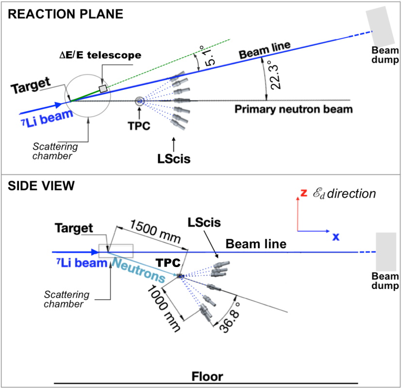
Figure 2: Schematic layout of the ReD experimental setup (not in scale). Upper panel is the view of the p(⁷Li,⁷Be)n reaction plane, lower panel is the side view. The primary ⁷Li beam travels along the $x$ axis and enters the vacuum scattering chamber which hosts the CH₂ target and the $\Delta E$/$E$ telescope. Neutrons emitted by the p(⁷Li,⁷Be)n reaction undergo elastic scattering inside the TPC and are eventually detected by one of the LScis of the neutron spectrometer, that are deployed within a cone of opening $\theta_{lsci}=36.8$° with respect to the target-TPC axis. See text for more details.

The conceptual layout of ReD is sketched in Fig. 2. The experiment deploys three detector systems: (1) a $\Delta E$/$E$ telescope made by Si detectors, to identify ⁷Be nuclei associated with neutrons; (2) the TPC to detect the Ar NRs; (3) a neutron spectrometer made by 7 LSci detectors to detect the neutrons scattered off Ar. The detectors of the neutron spectrometer are placed along the base circumference of a cone with axis corresponding to the target-TPC line (i.e. the direction of the incoming neutron), vertex on the TPC center and opening angle $\theta_{lsci}$. Therefore, all LScis detect neutrons which undergo elastic scattering on Ar at the same angle and hence produce NRs of the same energy $E_{r}$. While the NRs tagged by the seven individual LScis all have the same energy $E_{r}$, their momenta $\vec{p}_{r}$ form a different angle $\theta_{r}$ with respect to the TPC electric field ($z$ axis in Fig. 2), as required to test the directional effect. As it is important for this work to test the response to NRs also at $\theta_{r}=180$°, the TPC is placed at a different level with respect to the target, such to provide the incoming neutron with a momentum component along the field direction.

Once the angle $\theta_{tpc}$ between the primary ⁷Li beam direction and the target-TPC direction and the angle $\theta_{lsci}$ are fixed by the setup geometry, ReD is tuned to select mono-energetic Ar recoils of energy $E_{r}$ by the triple coincidence between the Si telescope, the TPC and the neutron spectrometer. The operational parameters chosen for ReD are $\theta_{tpc}=22.3$° and $\theta_{lsci}=36.8$°. The target-TPC distance and the TPC-LSci distance are 150 and 100 cm respectively, as a reasonable compromise between angular resolution and solid angle coverage: in both cases the uncertainty on the neutron direction is driven by the dimensions of the TPC and of the LSci, i.e. by the uncertainty on the interaction point within them. Keeping the geometry fixed, the energy $E_{r}$ of the NR can be changed by varying the primary beam energy. The ReD experimental layout was designed to allow for the measurements of NRs in the range of interest for dark matter direct searches, between 20 and 100 keV: this can be achieved by varying the energy of the primary ⁷Li beam between 20 and 34 MeV.

3.1 ⁷Li beam and target

The primary ⁷Li beam is produced by the 15 MV TANDEM accelerator of the INFN LNS CIAVOLA199364 at an energy of 28 MeV. The TANDEM offers an excellent resolution in the delivered energy, which is about 1% FWHM in our case. The data reported in this work were collected between January 31^st and February 14^th, 2020. The current of the ⁷Li beam ranged between 5 and 15 nA, corresponding to $1-3\cdot 10^{10}$ (⁷Li/s). The beam is driven to a vacuum scattering chamber, which hosts the CH₂ target and the $\Delta E$/$E$ telescope. Upstream the target, the ⁷Li beam is collimated to obtain a spot of 2 mm diameter at the target position. Neutrons are produced via the p(⁷Li,⁷Be)n reaction. The $\Delta E$/$E$ telescope detects the ⁷Be accompanying the neutrons that travel towards the TPC. As the accelerator does not allow the production of a pulsed beam, the direct detection of ⁷Be represents the best solution for event-by-event neutron tagging. The requirement to detect ⁷Be drives the choice of inverse kinematics (i.e. ⁷Li beam on a hydrogenous target) Drosg1981 ; Dave1982 , instead of the direct kinematics approach (proton beam on a ⁷Li target) employed by other experiments, as SCENE Cao:2015ks .

The targets of CH₂ have thickness ranging between 150 and 350 µg/cm², which is thin enough to allow for the escape of ⁷Be. Due to aging effects, each target was used for about 12 hours of data taking, before being replaced by means of a 12-target holder system placed inside the vacuum scattering chamber.

After the target, the ⁷Li beam travels straight forward towards a Ta beam dump placed 3 m downstream (see Fig. 2). Such a long distance is functional to minimize the background on the ReD setup due to the beam interaction on the beam dump. The beam intensity was precisely measured every few hours of operation by a Faraday Cup deployed about 30 cm downstream the target. However, the Faraday Cup was removed during the data taking, in order to reduce the background radiation close to the TPC. The continuous monitoring of the beam intensity was performed by measuring the rate of the ⁷Li elastic scattering on a dedicated Si detector (not shown in Fig. 2) placed at $\theta=7$° with respect to the beam line, where no ⁷Be is allowed by kinematics.

4 The detectors

4.1 The $\Delta E$/$E$ telescope

Neutrons directed towards the TPC  are produced in association with ⁷Be nuclei of energy $E_{Be}=19.0$ MeV and emitted at angle $\theta_{Be}=5.1$°. ⁷Be is detected by a dedicated $\Delta E$/$E$ telescope placed in the scattering chamber at a distance of $46\text{\,}\mathrm{c}\mathrm{m}$ from the CH₂ target. The telescope is made of two Si detectors manufactured by ORTEC, having thickness of 20 µm and 1000 µm, respectively; the ⁷Be loses about 7.6 MeV crossing the thinner stage and it is stopped in the thicker one. The detectors have a 100% efficiency for light charged particles detection and energy resolution of about 1%. The telescope is collimated using an Al shield with a hole of 2 mm diameter. For the fine tuning of the position, the telescope holder is mounted on a two axis remotely-controlled stepper motor which can operate in vacuum. The detectors are readout from a standard spectroscopic chain made by a pre-amplifier and a charge-sensitive amplifier, with 1 µs shaping time.

The combined measurement of $\Delta E$ and $E$ provides the discrimination in $Z$, which is necessary to distinguish the interesting Be from the far more abundant elastically-scattered Li.

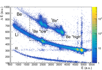
Figure 3: $\Delta E$ vs. $E$ scatter plot obtained from the irradiation of a CH₂ target with a 28-MeV ⁷Li beam. The bands identify nuclei of different $Z$ ($\alpha$, Li and Be), as discussed in the text. Neutrons traveling towards the TPC are produced in association with the ⁷Be nuclei of the locus labeled as “⁷Be low”. The dashed lines show the thresholds used in the normal operating conditions for the $\Delta E$ and $E$ detectors, and which are meant to suppress the dominant contribution from Li.

Fig. 3 shows the $\Delta E$ vs. $E$ scatter plot, upon the irradiation of the CH₂ target with the ⁷Li beam. The central, and most intense, band is created by Li ($Z=3$), mostly by elastic scattering on H and C. The uppermost band is due to Be ($Z=4$). As the reaction p(⁷Li,⁷Be)n occurs in inverse kinematics, two different solutions at the same angle $\theta_{Be}=5.1$° are allowed, with ⁷Be having energy of 19.0 MeV (“low energy”) and 20.4 MeV (“high energy”), respectively. Neutrons in association with the “low energy” ⁷Be are those travelling towards the TPC ($\theta_{n}=22.3$°), with $E_{n}=7.3$ MeV kinetic energy. The “high energy” ⁷Be is associated with neutrons of $E_{n}=2.7$ MeV emitted at $\theta_{n}=44$°: these neutrons do not hit directly the TPC, but can contribute to accidental coincidences due to scattering on the floor or on the walls. In Fig. 3 the loci from the two ⁷Be solutions are visible and clearly separated; the population between them is due to the inelastic interaction p(⁷Li,⁷Be*)n’, which also emits a neutron. Because of the finite extension of the beam spot and of the beam angular divergence, neutrons associated with the ⁷Be* detected at $\theta_{Be}$ can still travel inside the TPC and produce an interaction; they also contribute to the diffuse background, e.g. upon scattering on the walls or on the floor of the experimental area.

In order to suppress the dominant contribution from ⁷Li elastic scattering, the thresholds for the $\Delta E$ and $E$ detectors, shown in Fig. 3 as dashed lines, are used during the data acquisition. Fig. 4 displays the $\Delta E$ vs. $E$ scatter plot, acquired with the thresholds of Fig. 3, without (color) and with (dots) the requirement of coincidence with an event in the TPC compatible with a neutron interaction and within a 200 ns gate. As expected, neutron events in the TPC are mostly associated with a “low-energy” ⁷Be nucleus detected by the Si telescope. The dashed red box represents the ⁷Be selection cut used in the following analysis and described in Sect. 5.2.

Figure 4: $\Delta E$ vs. $E$ distribution obtained from the irradiation of a CH₂ target with a 28-MeV ⁷Li beam (color scale). The black dots are the events detected by the Si telescope in coincidence (within 200 ns) with an S1 signal in the TPC having a time profile compatible with a neutron-induced interaction. The dashed red box represents the ⁷Be selection cut used in the following analysis and described in Sect. 5.2. Inset: distribution of the time difference $\Delta t$ between TPC and Si telescope for events within the 200 ns coincidence gate.

4.2 The Time Projection Chamber

The heart of the ReD system is the dual-phase Ar TPC, whose detailed description and performance are reported in Agnes:2021zyq . It is a cubic volume of $5\times 5\times 6$ cm³, delimited on the side walls by acrylic plates interleaved with specular reflector foils, and the top and bottom by two transparent acrylic windows. The top and bottom windows are coated with a thin transparent conductive layer (indium-tin oxide, ITO), so they can be given an electric potential and be operated as anode and cathode, respectively. The extraction grid is a stainless steel mesh, having 95% optical transparency; it is located 10 mm below the anode window and it is kept electrically grounded. All internal surfaces are coated with a wavelength shifter (tetraphenyl-butadiene, TPB): it converts the UV light emitted by Ar scintillation (128 nm) into visible light, which better matches the sensitivity of typical photosensors. The lower part of the TPC contains LAr: the liquid fills the entire volume between the cathode and the extraction grid, plus 3 mm above the grid. The gas pocket is produced by means of a heater and it occupies the 7-mm thick region between the liquid surface and the anode.

The TPC electric fields which are set for this work are: drift field ($\mathcal{E}_{d}$) of 152 V/cm; extraction field ($\mathcal{E}_{ex}$) of 3.9 kV/cm; and electroluminescence field ($\mathcal{E}_{el}$) of 5.9 kV/cm. The maximum drift time is about 66 µs: this is the time required for an electron produced at the cathode to travel until the liquid surface. Due to a continuous recirculation loop of the liquid through a SAES getter, the purity of argon is such that the electron life time before capture by electronegative impurities is $>1$ ms, i.e. much longer than the 66-µs maximum drift time Agnes:2021zyq . The extraction field is strong enough to give a 100% extraction efficiency of the electrons from the liquid to the gas phase Chepel:2012sj .

After the UV photons from scintillation and electroluminescence of Ar are shifted to the visible range by the TPB coating, they can be detected by customised NUV-HD-Cryo Silicon PhotoMultipliers (SiPMs) from Fondazione Bruno Kessler, which can be operated at cryogenic temperature Gola:2019idb . The SiPMs are assembled in two $5\times 5$ cm² tiles, each containing 24 devices of dimensions 11.7 mm$\times$7.0 mm and arranged in a $4\times 6$ array. The tiles are placed behind the top and bottom acrylic windows of the TPC, providing a 30% total optical coverage. As the position of the S2 event in the gas phase can be used to estimate the $x-y$ coordinate of the original interaction point in the TPC, the SiPMs of top tile are readout in 22 channels for improved resolution: 20 SiPM are readout individually, while 4 lateral SiPMs are summed in pairs and grouped into two readout channels. The SiPMs of the bottom tiles are summed in groups of twelve, hence giving two readout channels. Two custom-made Front-End Boards (FEB) supply power to the SiPMs and amplify the output signals at cryogenic temperature. The SiPMs are operated at $+7\text{\,}\mathrm{V}$ of overvoltage with respect to the breakdown voltage. Due to the presence of resistors in the bias chain, the effective overvoltage of the SiPMs gets smaller than the nominal $+7\text{\,}\mathrm{V}$ when the bias current of the devices is high. This typically happens when the SiPMs are exposed to a significant amount of light, e.g. due to the high interaction rate under beam irradiation, and causes a change in the SiPM response (see Sect. 5.1).

More details about the cryogenic setup, the TPC, the photosensors and the readout system can be found in Agnes:2021zyq .

4.3 The neutron spectrometer

The neutron spectrometer used in ReD is made of seven 3-inch liquid scintillator (LSci) cells, individually read-out by photomultipliers (PMTs). The assembly includes the liquid scintillator cell, a ETL-9821B PMT and the front-end electronics with the amplifier. The cells are filled with the EJ-309 liquid scintillator by Eljen Technologies, which features a very powerful neutron-$\gamma$ discrimination based on the time pattern of the scintillation pulse.

The neutron detection efficiency of the detectors was measured individually by using a ²⁵²Cf source Stevanato2014 ; simophdthesis and found to be about 28% for the 7-MeV neutrons of interest for this work. The calibration of the energy scale was performed with $\gamma$-ray sources (²⁴¹Am, ¹³⁷Cs and ²²Na). Dedicated measurements taken with the annihilation $\gamma$-rays from the ²²Na source confirmed the time resolution to be better than 1 ns (rms).

The scintillators identify Ar recoils of the same energy but different angles $\theta_{r}$ with respect to the TPC drift field $\mathcal{E}_{d}$: $\theta_{r}$=180°(one LSci), 90°(two LScis, read out individually and labeled as “90°$l$” and “90°$r$”), 40°(two LScis, summed) and 20°(two LScis, summed).

4.4 Data acquisition and control infrastructure

The output signals from all of the detectors are sent to CAEN V1730 Flash ADC Waveform Digitizers and digitized with 14-bit resolution at a sampling rate of 500 MHz. In total a signal of 100 µs (50k samples) is acquired at each trigger: this is sufficiently long to contain the S1 and S2 signals of the TPC, given the maximum drift time of 66 µs for events occurring close to the cathode. About 10% of the digitization window is reserved for the pre-trigger. Two 16-channel CAEN V1730 boards were used for the measurement, synchronized with a daisy chain.

The data acquisition (DAQ) software was built upon a package developed for the PADME experiment Leonardi_2017 and based on the CAEN Digitizer Libraries. The trigger logic is implemented by means of an external NIM logic module as:

$$\texttt{SiTel}\land(\texttt{TPC}\lor\texttt{LScis})$$ (22)

where: SiTel, TPC and LScis are the trigger signals from the Si telescope, the TPC and the neutron spectrometer, respectively. The Si telescope trigger (SiTel) is built as the coincidence of the $\Delta E$ and $E$ detectors, with the thresholds displayed in Fig. 3. The TPC trigger (TPC) consists in the logical AND between the two readout channels of the bottom tile within a coincidence gate of 200 ns, in order to suppress the dark rate Agnes:2021zyq . The individual thresholds are set to approximately 2 PE. The TPC is expected to trigger with 100% efficiency on S1 signals from the $E_{r}=72$ keV NR events ($\textrm{S1}\sim 190$ PE) which are of interest for this work, although trigger inefficiencies can possibly come from pile-up. Finally, the neutron spectrometer trigger (LScis) is produced by the logical OR of the five readout channels of the seven scintillators. The energy threshold of each cell is set to approximately 20 keV_ee (electron equivalent), which corresponds to about 200 keV for a proton recoil Stevanato2014 . This is sufficient to have a nearly-100% trigger efficiency for the neutron events of interest, as their elastic scattering on the scintillator produces protons of average energy $\sim 3.6$ MeV, giving a 1.1 MeV_ee signal Stevanato2014 .

All detectors and sensors of the setup can be operated and read out remotely by means of a slow control system made of a suite of LabVIEW-based LabView applications. All parameters under control (e.g. temperatures, bias voltages, leakage currents) are monitored continuously, and readings are stored in a database every 10 s.

5 Event processing and selection

5.1 Event reconstruction and calibrations

The raw data from the TPC are the digitized waveforms of each of the SiPM channels, from which the event type, time, and 3D position were reconstructed following the procedure described in Agnes:2021zyq . The waveforms of all SiPM channels were baseline-subtracted, equalized according to the individual gains and summed. The summed waveform was filtered with a $20\text{\,}\mathrm{ns}\text{/}$ moving average window and then scanned by a dedicated pulse-finder algorithm, to search for possible S1 and S2 signals. Each pulse was classified as either S1 or S2 by using the pulse shape parameter $f_{\mathrm{p}}$, defined as the ratio of the charge in the first $700\text{\,}\mathrm{ns}\text{/}$ over the total charge: pulses with $f_{\mathrm{p}}<0.2$ are classified as S2. The total charge was then normalized according to the Single Electron Response (SER) of each SiPM channel, so to provide the S1 and S2 in units of PE. The pulse-finder algorithm is fully efficient for S1 signals above a few keV. The time delay between the S1 and S2 pulses, i.e. the electron drift time $t_{\mathrm{drift}}$, was used to estimate the $z$ coordinate of the interaction below the liquid-gas interface. Events with a single S1 pulse and a S2 pulse with $t_{\mathrm{drift}}$ between $6\text{\,}\mathrm{\SIUnitSymbolMicro s}\text{/}$ and the maximum drift time were kept for the subsequent analysis. The cut $t_{\mathrm{drift}}>$6\text{\,}\mathrm{\SIUnitSymbolMicro s}\text{/}$$ removes the events produced just below the extraction grid of the TPC, in which the S1 and S2 pulses are piled-up. The approximate $x-y$ position of the event was evaluated as the charge-weighted center of the S2 signal in the top SiPM array. The parameter $f_{\mathrm{p}}$ defined above was also used to perform the NR/ER discrimination: S1 pulses with $f_{\mathrm{p}}>0.4$ are selected as from NR. This simple cut was shown to allow for a NR/ER separation better than $2~{}\sigma$ for S1 above 50 PE Agnes:2021zyq .

The SER and the duplication factor $K_{\mathrm{dup}}$ were studied by irradiating the SiPMs with a 403-nm laser source and by modeling the photon counting statistics according to the Vinogradov distribution vinogradov2009 . The calibration was performed channel by channel, as described in Agnes:2021zyq . Typical values of $K_{\mathrm{dup}}$, which is the average number of secondary PEs produced by cross-talk and afterpulsing by each genuine primary photon on the SiPM, are between 0.31 and 0.37. The PE gain is corrected to remove cross-talk and afterpulsing according to the ratio $\frac{1}{1+K_{\mathrm{dup}}}$. Dedicated laser calibrations were taken every 12 hours throughout the beam time to monitor the stability of the SiPMs.

As mentioned in Sect. 4.2, the voltage drop in the bias resistor chain causes a reduction of the bias voltage of the SiPMs, which is proportional to the bias current and must be properly accounted for in the data analysis. The bias current registered during the laser calibrations by the slow control system was $<$0.5\text{\,}\mathrm{\SIUnitSymbolMicro A}\text{/}$$. During the beam irradiation, because of the much higher interaction rate and the much higher amount of light hitting the SiPMs, the bias current ranged up to 90 (150) µA for the bottom (top) SiPMs, depending on the intensity of the primary ⁷Li beam, which was not constant in time. To derive the corrections to the SER for each individual SiPM, three dedicated laser runs in which the TPC was simultaneously irradiated with high-activity radioactive sources were performed. The typical correction is of the order of $0.5\%\cdot I$, where $I$ is the bias current in µA. For this reason, the SER and $K_{\mathrm{dup}}$ correction was time-dependent and calculated using the closest reading of the bias current registered by the slow control. Besides the SER and $K_{dup}$, the photon detection efficiency also changes with bias voltage. A set of runs with ${}^{241}\mathrm{Am}$ $60\text{\,}\mathrm{keV}\text{/}$ $\gamma$ and the ${}^{7}\mathrm{Li}$ beam irradiation was performed to calibrate the additional bias current dependency in PE yield after the SER and $K_{\mathrm{dup}}$ correction.

The performance of the TPC was characterized prior to the irradiation, in a dedicated campaign Agnes:2021zyq . Specifically, the scintillation gain and ionization amplification of the TPC were measured to be $g_{1}=(0.194\pm 0.013)$ PE/photon and $g_{2}=(20.0\pm 0.9)$ PE/electron, respectively. Additional calibrations with ²⁴¹Am were taken daily during the campaign at LNS. These measurements confirm a light yield of $(8.53\pm 0.19)$ PE/keV at 60 keV and at $\mathcal{E}_{d}$=150 V; this is very well consistent with the expectation of 8.6 PE/keV based on the parametrization obtained in the pre-irradiation campaign Agnes:2021zyq .

The daily calibration runs with ²⁴¹Am were used to evaluate the dependence of the TPC response on the interaction position, and to determine the correction factors for S1 and S2, to be later applied to the physics runs. The events featuring one single S1 and one single S2 and having S1 compatible with the full energy deposition of the 60 keV $\gamma$-ray from ²⁴¹Am were grouped in a $22\times 11$ mesh, according to the interaction position in the TPC. The mesh has 22 entries in $x-y$, based on the top SiPM channel detecting the largest fraction of the S2 signal, and 11 bins in $z$, equally spaced between $t_{\mathrm{drift}}=$6\text{\,}\mathrm{\SIUnitSymbolMicro s}\text{/}$$ and $72\text{\,}\mathrm{\SIUnitSymbolMicro s}\text{/}$.

Firstly, S2 was corrected to account for the presence of impurities in LAr, which can cause the absorption of electrons during their drift path. The electron life time was estimated with an exponential fit of the S2 vs. $t_{\mathrm{drift}}$ profile, restricted to the events in the central eight $x-y$ bins. The $z$ dependency of S1 and S2 was further corrected by using a set of 5th-order polynomials S1${}_{i}(t_{\mathrm{drift}})$ and S2${}_{i}(t_{\mathrm{drift}})$: they are calculated by interpolating over the $z$-points within each bin $i$ in $x-y$. Three examples are shown in Fig. 5: the correction vs. $z$ is within 10-15%, for both S1 and S2. No significant variation in the position correction was found throughout the sequence calibration runs. Position dependencies mostly result from non-uniformity in the light collection efficiency within the TPC: as a consequence, the same corrections for S1 and S2 derived from ²⁴¹Am (ER) events were also applied to NR events.

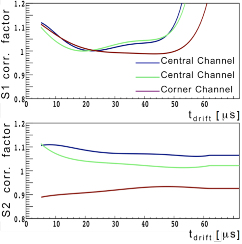
Figure 5: Examples of correction factors for the $z$ position dependence for events located below two central SiPMs (blue and green) and below one corner SiPM (red). Upper (lower) panel: correction factor for S1 (S2).

A simpler processing was performed for the digitized waveforms from the liquid scintillators and from the Si detectors of the telescope. The signal in the LSci detectors was processed by calculating the total charge, integrated within a gate of 600 ns. The ratio between the charge in the first 80 ns and the total was used as the discrimination parameter, resulting in a neutron-$\gamma$ discrimination better than $3\sigma$ above 200 keV_ee simophdthesis . The signals from the $E$ and $\Delta E$ detectors of the telescope were evaluated by taking the maximum of the digitized shaped waveforms from the charge-sensitive amplifier.

The time signal of all three kinds of detectors in the setup is critical for the coincidence event selection. The time stamp of a TPC event was defined as the zero-crossing time of the pulse obtained by passing the S1 pulse through a constant differential filter (CDF). The $\Delta E/E$ telescope generates two time stamps, one for the $\Delta E$ detector and one for the $E$ detector, which were both evaluated with CDFs. The reference time for the $\Delta E/E$ telescope used for the coincidence was taken as the average of the two time stamps. Finally, the time stamp for the neutron spectrometer was defined as the zero-crossing CDF time of the digitized waveforms.

5.2 Selection of signal events

The events of interest are triple coincidences between a ⁷Be nucleus detected in the $\Delta E$/$E$ telescope, and the two subsequent neutron scatterings in the TPC and in the neutron spectrometer.

A clean sample of signal events with the proper topology was selected through a sequence of cuts. Firstly, unambiguous TPC events were selected according to same criteria of Sect. 5.1: events with only one S1 and only one S2, separated by a $t_{\mathrm{drift}}$ within the range $[6,66]~{}$\mathrm{\SIUnitSymbolMicro s}\text{/}$$. An additional S2 “echo” signal, namely a secondary event due to photo-ionization of the cathode from the main S2 electroluminescence, is allowed in the time window $[67.5,72]~{}$\mathrm{\SIUnitSymbolMicro s}\text{/}$$ after the primary S2.

Afterwards, events in the TPC were selected by requesting that S1 is in time coincindence within a gate of 200 ns with the $\Delta E$/$E$ telescope and with one single LSci detector of the neutron spectrometer. In addition, neutron-induced (n,n’) events in the neutron spectrometer were efficiently selected by PSD against the dominant $\gamma$-ray background. The PSD based on the S1 signal of the TPC was not applied. This was meant to avoid an undesirable S1-dependent selection efficiency, given the fact that the discrimination based on $f_{\mathrm{p}}$ gets progressively worse for S1 signals below $100\text{\,}\mathrm{P}\mathrm{E}$.

The ⁷Be ion which accompanies the neutron traveling towards the TPC was selected by a combined cut on $\Delta E$ and $E$, which is shown in Fig. 4 (red dashed contour). The selection is not sensitive enough to resolve between the ⁷Be  emitted at the ground state in the p(⁷Li,⁷Be)n reaction and ⁷Be* in the first excited state coming from the p(⁷Li,⁷Be*)n’ reaction. Therefore, the neutron energy distribution consisted of two different mono-energetic components.

The data sample was further selected by using the time-of-flight (ToF) of the TPC with respect to the $\Delta E$/$E$ telescope, namely by keeping the events in which the delay between the telescope and the TPC (see inset in Fig. 4) is consistent with the flight time of the neutrons. The coincidence window in ToF was set to be S1-dependent, in order to ensure a S1-independent selection efficiency. The boundaries of the coincidence window were defined as the 1% and 99% quantiles in each S1 slice of 10 PE, after the subtraction of the constant background due to random neutrons and $\gamma$-rays. The random background contributes to about $1\text{\,}\mathrm{\char 37\relax}\text{/}$ of the events in the coincidence windows.

The coincidence windows for the delay $\Delta t(\mathrm{LSci}-\mathrm{SiTel})$ between the LSci and the telescope in triple-coincidence events were set with very stringent cuts, so to guarantee the selection of pure single-scattering neutron interactions. The timing of the individual LScis was calibrated by using as a reference the $\gamma$-rays produced in the TPC by inelastic interactions (n,n’$\gamma$) and then detected in the LScis: all $\gamma$ peaks were aligned to $\Delta t(\mathrm{LSci}-\mathrm{SiTel})=0$, as displayed in Fig. 6, where the effect of used cuts applied sequentially is shown. The single-scattered neutron events of interest form the peak around $20\text{\,}\mathrm{n}\mathrm{s}$. The low-statistics peak at about $25\text{\,}\mathrm{n}\mathrm{s}$ comes from the lower-energy neutrons produced in the p(⁷Li,⁷Be*)n’ interactions, while the tails at longer times are mostly due to multi-scattered neutron background. Monte Carlo simulations indicate that the hump around $60\text{\,}\mathrm{ns}\text{/}$ is originated by the neutrons associated with the “high energy” ⁷Be, which reach the TPC after scattering on the floor or other passive structure. The peaks around $-35\text{\,}\mathrm{ns}\text{/}$ and $-20\text{\,}\mathrm{ns}\text{/}$ are $\gamma$-rays emitted by p(⁷Li,⁷Li*)p inelastic scattering. Gaussian fits to the peak around $20\text{\,}\mathrm{n}\mathrm{s}$ determined the position and width of the window, individually for each scintillator. As mentioned in Sect. 4.3, the LSci channels which selected NR events at $\theta_{r}=$20\text{\,}\mathrm{\SIUnitSymbolDegree}\text{/}$$ and $40\text{\,}\mathrm{\SIUnitSymbolDegree}\text{/}$ were each made from the analogue sum of the signals of two different detectors. Since the cable lengths for the two detectors at $20\text{\,}\mathrm{\SIUnitSymbolDegree}\text{/}$ were not properly matched, this introduced a split in the timing: the $\Delta t(\mathrm{LSci}-\mathrm{SiTel})$ distribution for the channel at $20\text{\,}\mathrm{\SIUnitSymbolDegree}\text{/}$ was hence fitted with a double Gaussian. The coincidence windows were defined according to the position $\mu$ and width $\sigma$ of the peaks from the Gaussian fits, as summarized in Table 1 and they are used to select the triple coincidence events. The coincidence windows were further extended by $5\text{\,}\mathrm{n}\mathrm{s}$ in order to include the slower neutrons from p(⁷Li,⁷Be*)n’. Side-bands were also defined to estimate the random coincidence rate in each channel, see Tab. 1.

Table 1: Coincidence and side-band windows in the ToF $\Delta t(\mathrm{LSci}-\mathrm{SiTel})$ for each LSci channel. $d$ is the total width of the coincidence window, $d=6\sigma+5$ ns.

Angle $\theta_{r}$ of the TPC NR	90°$l$	40°	0°	90°$r$	20°
Neutron peak $\mu$ [$\mathrm{n}\mathrm{s}$]	19.75	19.44	19.51	20.09	$\mu_{1}=17.18$, $\mu_{2}=20.44$
Timing resolution $\sigma$ [$\mathrm{n}\mathrm{s}$]	1.12	1.12	1.50	1.25	1.17
Coincidence window	$[\mu-3\sigma,\mu+3\sigma+$5\text{\,}\mathrm{n}\mathrm{s}$]$				$[\mu_{1}-3\sigma$, $\mu_{2}+3\sigma+$5\text{\,}\mathrm{n}\mathrm{s}$]$
Side-band window	$[-$20\text{\,}\mathrm{n}\mathrm{s}$-20d,-$20\text{\,}\mathrm{n}\mathrm{s}$]\cup[$70\text{\,}\mathrm{n}\mathrm{s}$,$70\text{\,}\mathrm{n}\mathrm{s}$+20d]$

The triple coincidence events eventually considered for the statistical analysis of Sect. 6 are those which pass the sequence of cuts displayed in Fig. 6 and the additional selection in the $\Delta t(\mathrm{LSci}-\mathrm{SiTel})$ ToF from Table 1.

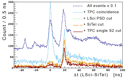
Figure 6: Timing spectra of $\Delta t(\mathrm{LSci-SiTel})$. All channels of the neutron spectrometer are aligned with the $\gamma$ peak at $t=0$. Cuts are applied accumulatively starting from the raw distribution (dark blue dashed histogram).

6 Statistical analysis

The S2 vs. S1 distribution of the NR events in the TPC which pass the selection procedure of Sect. 5.2 is displayed in Figure 7: the pink dots represent the events selected requiring the triple coincidence (TPC, Si telescope and neutron spectrometer); the colour-coded distribution includes the events in double coincidence (TPC and telescope). The triple coincidence sample contains about 650 NR events with S1 above $20\text{\,}\mathrm{P}\mathrm{E}$, which were collected during 10.7 live days of beam run. The double coincidence events constitute a large sample of about 70000 TPC NR events in all directions: they were hence used as a calibration data set to constrain the nuisance model parameters in the global fit below. Since the triple coincidence events are a small fraction of the double coincidences, the large sample of double coincidence events was also used as the template for random coincidence background.

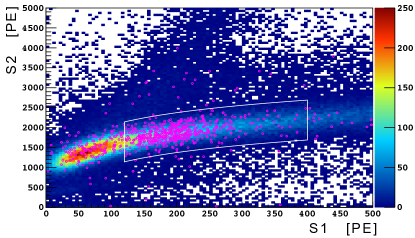
Figure 7: S2 vs. S1 distribution of NR events in the TPC. The color-coded histogram includes the event in double coincidence (TPC and telescope), namely at all angles $\theta_{r}$ with respect to the electric field. The pink circles are the events in triple coincidence (TPC, telescope and spectrometer). All corrections and cuts are applied. The white contour is the fit range in the (S1,S2) plane used for the statistical analysis described in Sect. 6.

The data samples were statistically analysed in order to evaluate the best estimate of the directionality parameter $\delta R=R-1$, which measures how much the shape of the initial ionization charge cloud differs from a sphere. As the number of events is relatively modest, an unbinned profile likelihood was applied. The global likelihood $\mathcal{L}$ is written as a product of three likelihood terms:

$$\mathcal{L}(\boldsymbol{X}\,|\,\delta R,\boldsymbol{\nu}) = \prod_{i=1}^{5}\mathcal{L}_{i}(\boldsymbol{X}_{i}\,|\,\delta R,\theta_{r}^{(i)},\boldsymbol{\nu})$$ (23)

$$\times\mathcal{L}_{\mathrm{cali}}(\boldsymbol{X}_{\mathrm{cali}}\,|\,\boldsymbol{\nu})\times\mathcal{L}_{\mathrm{constraint}}(\boldsymbol{\nu}),$$

where the product over $i$ refers to the five samples taken at the five angles $\theta_{r}^{(i)}={0^{\circ},20^{\circ},40^{\circ},90^{\circ}l,90^{\circ}r}$ of Tab. 1, each containing the observed array of events $\boldsymbol{X}_{i}=(\mathrm{S1},\mathrm{S2})$; $\delta R$ is the parameter of interest (POI); $\boldsymbol{\nu}$ is the array of nuisance parameters; $\boldsymbol{X}_{\mathrm{cali}}$ is the array of calibration data set. The POI is constrained in this work to $\delta R\geq 0$, as negative values of $\delta R$ are not physically allowed by the recombination model Cataudella:2017kcf . The three likelihood terms of Eq. 23 are described in detail below.

$\mathcal{L}_{i}$ is the extended likelihood of each sample of NR events at the recoil angle $\theta_{r}^{(i)}$:

$$\mathcal{L}_{i}=\mathrm{Poisson}(n_{i}|\hat{n_{i}})\prod_{X_{j}\in\boldsymbol{X}_{i}}\mathcal{P}_{i}(\mathrm{S1}_{j},\mathrm{S2}_{j};\delta R,\theta_{r}^{(i)},\boldsymbol{\nu})$$ (24)

where $n_{i}$ and $\hat{n_{i}}$ are the size of $\boldsymbol{X}_{i}$ and its mean, respectively, and $\mathcal{P}_{i}$ is the joint probability density function (PDF) of the events (S1,S2). The PDF is made as the combination of three components, one for signal and two from backgrounds:

$$\mathcal{P}_{i}(S1,S2) = (1-\lambda_{1i})(1-\lambda_{2})F_{\mathrm{sig}}(E_{r})$$ (25)

$$\otimes P(\mathrm{S1},\mathrm{S2};\delta R,\theta_{r}^{(i)},\boldsymbol{\nu},E_{r})$$

$$+[\lambda_{1i}F_{\mathrm{bkg1}}(E_{r})+(1-\lambda_{1i})\lambda_{2}F_{\mathrm{bkg2}}(E_{r})]$$

$$\otimes P(\mathrm{S1},\mathrm{S2};\delta R,\bar{\theta}_{r},\boldsymbol{\nu},E_{r}).$$

The first component is the energy spectrum for the signal $F_{\mathrm{sig}}(E_{r})$, which depends on the recoil energy $E_{r}$, convolved with the response function $P$ of the TPC to mono-energetic NR events, as defined in Eq. LABEL:eq:TPCResponse. The parameters $\lambda_{1i}$ are the fractions of random coincidences within each data sample: they were estimated from the data, using the counting rate in the side-band in ToF and are listed in Tab. 2. Similarly, $\lambda_{2}$ is the scaling factor for multi-scattering background, namely the fraction of those events with respect to all NR events in the coincidence window. The other two components are the energy distributions of the backgrounds due to random coincidences, $F_{\mathrm{bkg1}}(E_{r})$, and to multiple neutron scattering, $F_{\mathrm{bkg2}}(E_{r})$. They are also convolved with the response function $P$ of the TPC.

In order to speed-up the computation of the response function $P$, the Poisson and binomial distributions are approximated by Gaussian distributions, such that the convolutions over $N_{\mathrm{ph}}$ and $N_{e^{-}}$ in Eq. LABEL:eq:TPCResponse can be evaluated analytically. As the angular distribution for background events is approximately random, the $\theta_{r}$ dependence of $f(\theta_{r},R)$ is averaged out by using the equivalent angle $\bar{\theta}_{r}$ calculated analytically for an isotropic distribution and the functional dependence on the angle is approximated as $\langle f(\theta_{r},R)\rangle\sim f(\bar{\theta}_{r},R)$. The factor $\lambda_{2}$ and the three energy spectra ($F_{\mathrm{sig}}$, $F_{\mathrm{bkg1}}$, and $F_{\mathrm{bkg2}}$) were evaluated by means of a dedicated Monte Carlo simulation using the Geant4-based framework g4ds Agostinelli:2003fg ; Allison:2006cd ; Allison:2016lfl ; Agnes:2017grb . The events from the simulations underwent the same sequence of selection cuts used for the real data. The energy distributions derived by the Monte Carlo are displayed in Fig. 8. The three energy distributions were then analytically parametrized in order to optimize the calculation of the CPU-intensive PDF $\mathcal{P}_{i}$. $F_{\mathrm{sig}}$ consists of two Gaussian peaks corresponding to the NR induced by neutrons from p(⁷Li,⁷Be)n and p(⁷Li,⁷Be*)n’. $F_{\mathrm{bkg1}}$ and $F_{\mathrm{bkg2}}$ were approximated by a double-exponential and a single exponential, respectively, whose parameters were calculated by fits to the Monte Carlo distributions.

Table 2: Fraction of random coincidence events, $\lambda_{1i}$, in the range S1$\,\in[120,400]$\mathrm{P}\mathrm{E}$$ and S2$\,\in[800,2800]$\mathrm{P}\mathrm{E}$$ in the five samples of triple-coincidence events at different $\theta_{r}$. Uncertainty is about 2% for all samples.

0°	20°	40°	90°$l$	90°$r$
0.045	0.048	0.047	0.026	0.041

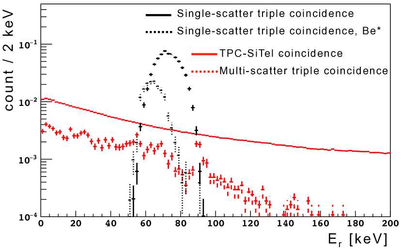
Figure 8: Signal and background spectra from g4ds Monte Carlo simulation. Solid and dotted black lines show the distribution of the NR energy $E_{r}$ for signal events associated with ⁷Be and ⁷Be^∗ neutrons, respectively. Solid red line shows the random coincidence background spectrum $F_{\mathrm{bkg1}}$ and the dashed red line the spectrum $F_{\mathrm{bkg2}}$ from multi-scattered triple coincidence events. The error bars represent the Monte Carlo statistical uncertainties.

The factor $\mathcal{L}_{\mathrm{cali}}$ of the global likelihood of Eq. 23 is the constraint term on the nuisance parameters and it depends on the events $\boldsymbol{X}_{\mathrm{cali}}$ in the calibration set (i.e. colour-coded histogram in Fig. 7) While the energy spectrum of the calibration events is a broad and featureless distribution, the joint distribution of the NR band in the (S1,S2) plane can set a strong constraint on the nuisance parameters. Since the fraction of signal events in the calibration sample is negligible, the energy distribution is well approximated by the random background $F_{\mathrm{bkg1}}$. The calibration term is hence written as:

$$\mathcal{L}_{\mathrm{cali}}=\prod_{X_{j}\in\boldsymbol{X}_{\mathrm{cali}}}P(\mathrm{S1}_{j},\mathrm{S2}_{j};\delta R,\bar{\theta}_{r},\boldsymbol{\nu},E_{r})\otimes F_{\mathrm{bkg1}}(E_{r}).$$ (26)

In order to avoid any analysis bias, $\delta R$ should be decoupled from the nuisance parameters as much as possible. The explicit occurrence of the POI $\delta R$ in Eq. 26 is due to the fact that the parameter $\xi_{m}$ in the modified Thomas-Imel model in Eq. 5 is dependent on $\delta R$ because of the track length. To remove such undesirable degeneracy, the angular dependence term and the Thomas-Imel parameter were re-defined as

$$f^{\prime}(\theta_{r},R)=f(\theta_{r},R)/f(\bar{\theta}_{r},R)$$ (27)

and

$$\xi_{m}^{\prime}=\xi_{m}/f(\bar{\theta}_{r},R),$$ (28)

respectively. In this way the angle-averaged position of the NR band in calibration data does not depend on $\delta R$ and the POI $\delta R$ is left as a pure representation of directionality. Furthermore, the degenerate nuisance parameters were re-cast into a unique nuisance parameter $A=\xi_{m}^{\prime}/(\mathcal{E}_{d}\cdot\langle N_{\mathrm{i}}\rangle)$, which represents the recombination probability of one electron-ion pair.

The last factor of the global likelihood, $\mathcal{L}_{\mathrm{contraint}}(\boldsymbol{\nu})$, is the pull term for the nuisance parameters which were known by prior independent measurements. Those parameters are constrained by Gaussian terms

$$\mathcal{L}_{\mathrm{constraint}}(\boldsymbol{\nu})=\prod_{i}\frac{1}{\sqrt{2\pi}\sigma_{\nu_{i}}}\exp{-\frac{(\nu_{i}-\nu_{i}^{0})^{2}}{2\sigma_{\nu_{i}}^{2}}}$$ (29)

based on the previously-measured values $\nu_{i}^{0}$ of the parameters $\nu_{i}$ and on their corresponding uncertainties.

Table 3: List of the parameters used in the model. $\delta R$ is the parameter of interest, while all others are nuisance parameters, constrained by the calibration data and/or by a Gaussian pull term. The error bars are the standard deviation which is taken in the Gaussian pull terms. The parameters reported without uncertainties are fixed. The gains $g_{1}$ and $g_{2}$ come from the previous TPC performance study Agnes:2021zyq . The S1 resolution of the TPC of Eq. LABEL:eq:TPCResponse is parametrized as $\sigma_{\mathrm{S1}}^{2}=\mathrm{S1}/[$\mathrm{P}\mathrm{E}$]+{\sigma^{*}_{\mathrm{S1}}}^{2}$, namely by the combination of the statistical term and of an extra contribution. The same is done for the S2 resolution.

	Constraint	Comment
$\delta R$	-	Parameter of interest
$A$	$0.04\pm 0.01$ $[$\mathrm{1}\mathrm{/}\mathrm{e}^{-}$]$	$A=e/[2\pi\epsilon_{r}\epsilon_{0}\mathcal{E}_{d}\sigma^{2}\mu_{-}f(\bar{\theta}_{r},R)]$
$k_{e}$	$2.8$	Electronic quenching coefficient Mei:2008ca
$W_{ph}$	$19.5$ $[$\mathrm{e}\mathrm{V}$]$	Energy for scintillation photon production Doke:2002oab
$N_{\mathrm{ex}}/N_{\mathrm{i}}$	$0.2\sim 2$	Excitation to ionization ratio. Energy dependence as in Cao:2015ks
$g_{1}$	$0.196\pm 0.020$ $[$\mathrm{P}\mathrm{E}\mathrm{/}\mathrm{p}\mathrm{h}$]$	S1 signal yield
$g_{2}$	$20.5\pm 2.5$ $[$\mathrm{P}\mathrm{E}\mathrm{/}\mathrm{e}^{-}$]$	S2 signal yield
$\sigma^{*}_{\mathrm{S1}}/\mathrm{S1}$	$0.003\pm 0.05$	S1 detector resolution in addition to $\sqrt{\mathrm{S1}}$
$\sigma^{*}_{\mathrm{S2}}/\mathrm{S2}$	$0.001\pm 0.05$	S2 detector resolution in addition to $\sqrt{\mathrm{S2}}$
$\lambda_{1}$	Table 2	Fraction of random coincidence
$\lambda_{2}$	0.16	Ratio of multi-scattering to all NR in coincidence windows

As a summary, the parameters and their reference values are summarized in Tab. 3. The recombination probability $A$ depends on $\sigma$, the size of the ionization cluster of Eq. 4, which is dominated by the electron diffusion during thermalization. Due to their high mobility and long thermalization time, electrons diffuse for a few µm in LAr Wojcik:2003ja ; mozumder1995free . It is found that $A=0.04/e^{-}$, which corresponds to $\sigma=$1.8\text{\,}\mathrm{\SIUnitSymbolMicro m}\text{/}$$, was an appropriate initialization parameter for the likelihood fit. The ratio $N_{\mathrm{ex}}/N_{\mathrm{i}}$ was treated as a function of recoil energy, according to the indications by SCENE Cao:2015ks . The TPC gains $g_{1}$ and $g_{2}$ were estimated according to the TPC characterization in Agnes:2021zyq , and were treated as nuisance parameters in order to accommodate for possible variations in the TPC performance. The parameters $W_{ph}$, $k_{e}$, $\lambda_{1}$ and $\lambda_{2}$ were fixed in order to limit the degeneracies in the fit: their effect on the POI is minor and is accounted below as a systematic uncertainty.

Finally, experimental data of Fig. 7 (calibration and five triple-coincidence samples) were fitted against the model of Eq. 23. In order to make the fit stable the fit region in the (S1,S2) plane was selected in order to include only the NR band, with S1$\,\in[120,400]$\mathrm{P}\mathrm{E}$$, as represented by the white contour in Fig. 7. The S1 range corresponds to NR energies between approximately 35 and 150 keV, and hence comfortably includes the expected NR signal at $\sim 72$ keV. The low-S1 edge $S1>120~{}$\mathrm{P}\mathrm{E}$$ was set in order to avoid any inefficiencies in the event reconstruction and selection. The center of the NR band was empirically parametrized with the function S2$\,/[$\mathrm{P}\mathrm{E}$]=455\ln(\mathrm{S1}/[$\mathrm{P}\mathrm{E}$])-535$ and the cut was set as $\pm 500~{}$\mathrm{P}\mathrm{E}$$ in S2. The fit region globally contains 529 triple coincidence and 42340 calibration events.

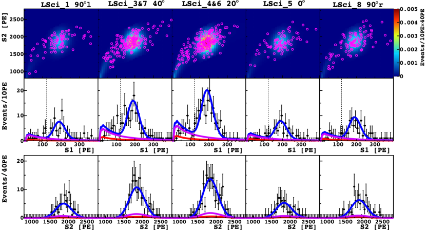
Figure 9: Experimental data superimposed with the best-fit model. The fit is performed for $S1\in[120,400]$\mathrm{P}\mathrm{E}$$ and within the white contour of Fig. 7. Upper row: S2 vs. S1 distribution for the calibration data set (color-coded histogram) and for the triple-coincidence data sets at different angles $\theta_{r}$ (pink circles). Middle row: projection on S1 for the triple-coincidence samples. The dashed vertical lines at $120$\mathrm{P}\mathrm{E}$$ mark the left edge of the fit range. Bottom row: projection on S2 for the triple-coincidence sample in the range of $S1\in[120,400]$\mathrm{P}\mathrm{E}$$. The blue, red and pink curves are the total spectrum, the random coincidence background $F_{\mathrm{bkg1}}$, and multi-scattering background $F_{\mathrm{bkg2}}$, respectively.

Table 4: Best-fit of the parameters and correlation coefficients between the nuisance parameters and the POI $\delta R$.

Parameter	Value	Correlation with $\delta R$
$\delta R$	$0.037\pm 0.027$	-
$A\,[$\mathrm{1}\mathrm{/}\mathrm{e}^{-}$]$	$(4.01\pm 0.06)\times 10^{-2}$	-0.014
$g_{1}\,[$\mathrm{P}\mathrm{E}\mathrm{/}\mathrm{p}\mathrm{h}$]$	$0.204\pm 0.002$	0.013
$g_{2}\,[$\mathrm{P}\mathrm{E}\mathrm{/}\mathrm{e}^{-}$]$	$20.1\pm 0.2$	-0.009
$\sigma^{*}_{\mathrm{S1}}$/S1	$0.017\pm 0.003$	-0.012
$\sigma^{*}_{\mathrm{S2}}$/S2	$0.0002\pm 0.0060$	0.026

The fit result is shown in Fig. 9 and reported in Tab. 4. The positions of the signal peak in both S1 and S2 (middle and bottom rows of Fig. 9) are mutually consistent among the five samples at different $\theta_{r}$. The best-fit for the POI is $\delta R=0.037\pm 0.027$, which is less than $2\sigma$ away from a null result; the uncertainty on $\delta R$ is largely driven by statistics. The upper limit of $\delta R$ is calculated by a toy Monte Carlo approach, in order to guarantee the correct coverage: it results to be $\delta R<0.072$ at 90% CL. The best-fits of the nuisance parameters are in good agreement with the central values of their estimates used for the constraints. In particular, the smallness of the best-fit for the parameters $\sigma^{*}_{\mathrm{S1}}$/S1 and $\sigma^{*}_{\mathrm{S2}}$/S2, which are the extra (non-statistical) contributions to the experimental resolution in S1 and S2, demonstrates that the spatial inhomogeneities of the detector response were properly corrected. Furthermore, the proper convergence and the absence of a significant bias for all fit parameters, notably including the POI $\delta R$, were checked by running a dedicated set of toy Monte Carlo simulations.

The uncertainties on $\delta R$ related to the nuisance parameters are automatically accounted in the fit. All other systematic uncertainties on $\delta R$, e.g. those related to the values of $W_{ph}$, $k_{e}$, $\lambda_{1}$ and $\lambda_{2}$, to the spectral shapes $F_{\mathrm{sig}}$, $F_{\mathrm{bkg1}}$ and $F_{\mathrm{bkg2}}$, and to the approximation of $\bar{\theta}_{r}$ from isotropic distribution, are globally evaluated to be an order of magnitude smaller than the statistical term and are hence neglected in this work.

7 Discussion

The results of this work suggest that the charge recombination in NRs in the energy range of interest for WIMP DM searches has a limited directional dependence. A possible explanation is that the directional effect is washed out in the isotropic thermalization process of the electrons: the range of $70\text{\,}\mathrm{keV}\text{/}$ argon ions in LAr, $0.18\text{\,}\mathrm{\SIUnitSymbolMicro m}\text{/}$ srim , is much shorter than the electron thermalization radius $r_{t}\sim$$2.5\text{\,}\mathrm{\SIUnitSymbolMicro m}\text{/}$ Wojcik:2003ja ; Wojcik:2016gy . If all electrons were confined within the Onsager radius, the recombination probability $A$ would be $8/e^{-}$, namely, two orders of magnitude higher than measured in this work. This indicates that the extension of the thermalized electron cloud is much bigger than the Onsager radius, thus weakening the initial directional effect. Other non-local processes at the length scale of a few µm can also contribute to the size of the electron cloud, including the emission of Auger electrons and fluorescence X-rays from excited Ar atoms estar ; xcom .

The strongest constraint on $\delta R$ from the fit comes from the position of the S2 peak, since $g_{2}\gg g_{1}$. In fact, the SCENE hint for directional sensitivity was primarily given by the 7% variation in S1 for NRs parallel and perpendicular to $\mathcal{E}_{d}$: no variation of S2 vs. direction was observed in SCENE. While the SCENE data were never analyzed according to the directional model of Cataudella:2017kcf , an asymmetry $\delta R\approx 2$ would be required to generate a 7%-effect on S1. However, given the anti-correlations of Eqs. 15 and 16, such a large $\delta R$ would produce a much more significant variation in S2 ($\sim 80\%$ between parallel and perpendicular directions), which is not observed in SCENE. The lack of a variation in the S2 signal, which is further confirmed in this work, rules out the directional modulation in charge recombination as the explanation of the effect and sets an upper limit on $\delta R$. Furthermore, the ReD data, with an improved signal yield and resolution in S1, do not confirm the variation in S1 at different directions which was reported by SCENE. As for S2, no statistically-significant variation was found for S1.

The LAr signal model adopted in this work has two major upgrades comparing to the models commonly used in the literature. The first modification is about charge recombination, by the introduction of the directional term of Eq. 5 from Ref. Cataudella:2017kcf . The second modification is the use of an energy-dependent ratio $N_{\mathrm{ex}}/N_{\mathrm{i}}$, which allows for a better fit of the NR band shape and improves significantly the performance of the likelihood fit. If $N_{\mathrm{ex}}/N_{\mathrm{i}}$ is kept constant to the value 1, which is commonly-adopted for NRs Doke:2002oab ; Hitachi:2021hac , the fit still returns a value of $\delta R$ compatible with zero, but the model fails to reproduce the shape of the S2 vs. S1 band and the S2 distribution for NRs; furthermore, the best-fit for $g_{2}$ in this case is $29.9\pm 0.1$ $\mathrm{P}\mathrm{E}\mathrm{/}\mathrm{e}^{-}$, which is in tension with the prior measurement of Table 3. While the SCENE data also support the energy dependence of $N_{\mathrm{ex}}/N_{\mathrm{i}}$, the physical motivation of it requires further study. One possibility is that this is the apparent effect of energy dependences in the nuclear quenching, electron quenching and recombination processes, which are unaccounted by the Lindhard, Mei and Thomas-Imel models used in this work. Specifically: the Thomas-Fermi screening function used in the Lindhard model is known to have a bias in the $O(10)$\mathrm{k}\mathrm{e}\mathrm{V}$$ range Bezrukov:2010qa ; Sigmund2004 ; the Mei model simplifies the average electronic stopping power by taking the value at the initial electron kinetic energy; the charge recombination model does not consider the dependence on the charge cloud size on the recoil energy. All these energy-dependent factors are not accounted in the models and they could eventually show up as an effective energy dependence in $N_{\mathrm{ex}}/N_{\mathrm{i}}$. It has anyhow a small effect on the systematic uncertainty on $\delta R$, due to the weak correlation reported in Tab. 4.

Taking the central value $\delta R=0.037$ from the fit, the amplitude of the S2 daily modulation curve, which results by folding the directional dependence S2$(\theta)$ of this work into the WIMP recoil direction distribution from Ref. Cadeddu:2017ebu , is only $0.5\text{\,}\mathrm{\char 37\relax}\text{/}$ peak-to-peak. Given the very large number of candidate events required to statistically identify it, this effect could hardly be of experimental use in a future $O(100)$ ton argon dual-phase TPC DM detector.

8 Conclusions

The Recoil Directionality (ReD) experiment was designed within the GADMC to explore the possible directional sensitivity of an Ar dual-phase TPC to nuclear recoils in the energy range of interest for WIMP DM searches. The ReD TPC was irradiated with neutrons of known energy and direction at the INFN, Laboratori Nazionali del Sud, in order to produce Ar recoils of about 70 keV kinetic energy. Nuclear recoils traveling in five different directions with respect to the drift field $\mathcal{E}_{d}$ of the TPC were selected using a neutron spectrometer made by liquid scintillation detectors. A statistical analysis based on the Cataudella et al. model Cataudella:2017kcf was performed to assess the TPC response for those samples of NR events.

The data from this work do not show any statistically-significant dependence of either S1 or S2 on the direction for NRs of $\sim 70$ keV. The best-fit for the parameter of interest $R$, which measures the aspect ratio between the long and short axes of the initial electron cloud, is $R=(1.037\pm 0.027)$, or $R<1.072$ at 90% CL. The absence of significant deviations from the spherical symmetry of the electron cloud indicates that the electron thermalization process likely plays a significant role in weakening any initial direction-induced anisotropy of the charge cloud.

Appendix A A data-driven analysis approach

The directionality analysis presented in this work depends on the specific model by Cataudella et al. Cataudella:2017kcf which was adopted to describe the phenomenon. One possibility to release such a model depencence and to validate the result is to employ a data-driven approach based on Machine Learning (ML) techniques. ML techniques are in fact very effective in revealing possible correlations between quantities in the study of phenomena for which large data samples are available, even if a model for their description is lacking.

Supervised learning algorithms were used to try to highlight the signature for possible directionality effects in the electron-ion recombination in the ReD  data noemipthesis . Due to the limited size of the triple coincidence event samples, an indirect approach was adopted, which makes use of all TPC calibration events. The data set of the double coincidence events provides a two-order-of-magnitude larger amount of data for the training of the model, and this is a desirable condition when working with ML algorithms.

In an ideal LAr TPC, the S2 signal is expected to be related to S1 through some functional form S2$=f$(S1). The basic assumption of this strategy is that the function $f$ does not depend on the direction of the Ar recoil, namely that the angle $\theta_{r}$ between the recoil and the drift field does not affect the balance between S1 and S2. Deviations from this trend would highlight a possible effect of the recoil directionality.

The model was derived by using the calibration data set, which is made of NR events characterized by a wide distribution of angles $\theta_{r}$. The data set contained about 72000 events and it was randomly split (70:30) in a training and testing set, on which the model was trained and tested, respectively. During the training phase, the algorithm built the function $f$ used to predict S2, event-by-event, based on the patterns which are learnt from the training set. Each pattern consists of a vector of features: S1 signal [PE], $x-y$  position [cm], and $t_{\mathrm{drift}}$[µs] as the $z$ coordinate of the event, within the appropriate ranges, and the measured S2 value as a target. The derived model aims to predict the value of the ionization signal S2, for each of the events, from the knowledge of S1 and of the reconstructed interaction point within the TPC.

The Extreme Gradient Boosting algorithm (xgboost) was used to derive the model XGB . To evaluate the accuracy of the model, the metric of the relative prediction error was adopted. This is defined, for the $i$-th pattern (i.e. the $i$-th event in the TPC), as

$$\epsilon_{pred}^{i}=\frac{\mathrm{S2}_{measured}^{i}-\mathrm{S2}_{predicted}^{i}}{\mathrm{S2}_{measured}^{i}}.$$ (30)

The trend of $\epsilon_{pred}^{i}$ was investigated for each event, and also against each feature describing the patterns, to verify that there were no regions in the feature space in which the model has a worse response that could introduce any bias in the predictions. At the end of the training phase, the model was able to provide a satisfactory prediction of the experimental S2 of the events in the testing set: the relative errors $\epsilon_{pred}^{i}$ resulted to be approximately Gaussian-distributed with mean 0.0043(6) and standard deviation 0.09.

Subsequently, the model was used to make predictions on the triple coincidence data set. For these data, the known $\theta_{r}$ values are used to check for possible directional-dependent deviations of the predicted S2 values compared to those measured experimentally. $\epsilon_{pred}^{i}$ was initially calculated for each event in the triple coincidence data set and the corresponding values were subdivided into four subsets, according to the angle $\theta_{r}$ determined by the coincident neutron detection. The mean value of $\epsilon_{pred}$ in each data set and the corresponding uncertainty are displayed in Fig. 10 as a function of the recoil direction $\theta_{r}$.

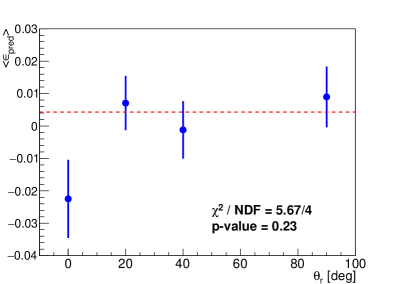
Figure 10: Mean relative prediction error for each $\epsilon_{pred}^{i}$ distribution obtained by splitting data into the four data sets. The red dashed line marks the level $\epsilon_{pred}=0.0043$ from the testing set (i.e. null directional effect).

The point at $\theta_{r}$ = $0\text{\,}\mathrm{\SIUnitSymbolDegree}\text{/}$ is lower than the others, as expected in the case of directionality effects, since traces parallel to $\mathcal{E}_{d}$ would result in enhanced S1 signals and reduced S2. Nevertheless, experimental data are compatible with the null hypothesis of no directionality effect: the $p$-value calculated from the $\chi^{2}$ test is 23%. Therefore, the data-driven analysis carried out using ML techniques on the data collected in the ReD TPC is compatible with the absence of any directional effect, in agreement with the analysis based on the model by Cataudella et al. Cataudella:2017kcf .

The DarkSide-20k Collaboration

P. Agnes¹, I. Ahmad², S. Albergo^{3 , 4} , I. F. M. Albuquerque⁵, T. Alexander⁶, A. K. Alton⁷, P. Amaudruz⁸, M. Atzori Corona⁹, M. Ave⁵, I. Ch. Avetisov¹⁰, O. Azzolini¹¹, H. O. Back⁶, Z. Balmforth¹², A. Barrado-Olmedo¹³, P. Barrillon¹⁴, A. Basco¹⁵, G. Batignani^{16 , 17} , V. Bocci¹⁸, W. M. Bonivento⁹, B. Bottino^{19 , 20 , 21} , M. G. Boulay²², J. Busto¹⁴, M. Cadeddu⁹, A. Caminata²⁰, N. Canci¹⁵, G. Cappello^{3 , 4} , A. Capra⁸, S. Caprioli^{19 , 20} , M. Caravati⁹, N. Cargioli^{23 , 9} , M. Carlini²⁴, P. Castello^{25 , 9} , V. Cataudella^{26 , 15} , P. Cavalcante²⁴, S. Cavuoti^{26 , 15} , S. Cebrian²⁷, J. M. Cela Ruiz¹³, S. Chashin²⁸, A. Chepurnov²⁸, E. Chyhyrynets¹¹, L. Cifarelli^{29 , 30} , D. Cintas²⁷, M. Citterio³¹, B. Cleveland^{32 , 33} , V. Cocco⁹, E. Conde Vilda¹³, L. Consiglio²⁴, S. Copello^{20 , 19} , G. Covone^{26 , 15} , M. Czubak³⁴, M. D’Aniello^{35 , 15} , S. D’Auria³¹, M. D. Da Rocha Rolo³⁶, S. Davini²⁰, A. de Candia ^{26 , 15} , S. De Cecco^{18 , 37} , D. De Gruttola^{38 , 39} , G. De Filippis^{26 , 15} , D. Dell’Aquila^{40 , 58} , S. De Pasquale^{38 , 39} , G. De Rosa^{26 , 15} , G. Dellacasa³⁶, A. V. Derbin⁴¹, A. Devoto^{23 , 9} , F. Di Capua^{26 , 15} , L. Di Noto^{19 , 20} , C. Dionisi^{18 , 37} , P. Di Stefano⁴², G. Dolganov⁴³, F. Dordei⁹, A. Elersich⁴⁴, E. Ellingwood⁴², T. Erjavec⁴⁴, M. Fernandez Diaz¹³, G. Fiorillo^{26 , 15} , P. Franchini^{45 , 12} , D. Franco⁴⁶, N. Funicello^{38 , 39} , F. Gabriele⁹, D. Gahan^{23 , 9} , C. Galbiati^{21 , 24 , 1} , G. Gallina²¹, G. Gallus⁹, M. Garbini^{47 , 30} , P. Garcia Abia¹³, A. Gendotti⁴⁸, C. Ghiano²⁴, C. Giganti⁴⁹, G. K. Giovanetti⁵⁰, V. Goicoechea Casanueva⁵¹, A. Gola^{52 , 53} , G. Grauso¹⁵, G. Grilli di Cortona¹⁸, A. Grobov^{43 , 54} , M. Gromov^{28 , 55} , M. Guan⁵⁶, M. Guerzoni³⁰, M. Gulino^{57 , 58} , C. Guo⁵⁶, B. R. Hackett⁶, A. L. Hallin⁵⁹, A. Hamer^{60 , 12} , M. Haranczyk³⁴, T. Hessel⁴⁶, S. Hill¹², S. Horikawa^{61 , 24} , F. Hubaut¹⁴, J. Hucker⁴², T. Hugues², An. Ianni^{21 , 24} , V. Ippolito¹⁸, C. Jillings^{32 , 33} , S. Jois¹², P. Kachru^{1 , 24} , N. Kemmerich⁵, A. A. Kemp⁴², C. L. Kendziora⁶², M. Kimura², I. Kochanek²⁴, K. Kondo^{61 , 24} , G. Korga¹², S. Koulosousas¹², A. Kubankin⁶³, M. Kuss¹⁶, M. Kuzniak², M. La Commara^{64 , 15} , M. Lai^{23 , 9} , E. Le Guirriec¹⁴, E. Leason¹², A. Leoni^{61 , 24} , X. Li²¹, L. Lidey⁶, M. Lissia⁹, L. Luzzi¹³, O. Lychagina⁵⁵, O. Macfadyen¹², I. N. Machulin^{43 , 54} , S. Manecki^{32 , 33} , I. Manthos⁶⁵, L. Mapelli²¹, A. Margotti³⁰, S. M. Mari^{66 , 67} , C. Mariani⁶⁸, J. Maricic⁵¹, A. Marini^{19 , 20} , M. Martínez^{27 , 69} , C. J. Martoff⁷⁰, G. Matteucci¹⁵, K. Mavrokoridis⁷¹, A. B. McDonald⁴², A. Messina^{18 , 37} , R. Milincic⁵¹, A. Mitra⁷², A. Moharana^{1 , 24} , J. Monroe¹², E. Moretti^{52 , 53} , M. Morrocchi^{16 , 17} , T. Mróz³⁴, V. N. Muratova⁴¹, C. Muscas^{25 , 9} , P. Musico²⁰, R. Nania³⁰, M. Nessi²⁴, G. Nieradka², K. Nikolopoulos⁶⁵, J. Nowak⁴⁵, K. Olchansky⁸, A. Oleinik⁶³, V. Oleynikov^{73 , 74} , P. Organtini²¹, A. Ortiz de Solórzano²⁷, L. Pagani⁴⁴, M. Pallavicini^{19 , 20} , L. Pandola⁵⁸, E. Pantic⁴⁴, E. Paoloni^{16 , 17} , G. Paternoster^{52 , 53} , P. A. Pegoraro^{25 , 9} , K. Pelczar³⁴, V. Pesudo¹³, S. Piacentini^{37 , 18} , N. Pino^{3 , 4} , A. Pocar⁷⁵, D. M. Poehlmann⁴⁴, S. Pordes⁶², P. Pralavorio¹⁴, D. Price⁷⁶, F. Ragusa^{77 , 31} , Y. Ramachers⁷², M. Razeti⁹, A. L. Renshaw⁷⁸, M. Rescigno¹⁸, F. Retiere⁸, L. P. Rignanese³⁰, C. Ripoli^{39 , 38} , A. Rivetti³⁶, A. Roberts⁷¹, C. Roberts⁷⁶, J. Rode^{49 , 46} , G. Rogers⁶⁵, L. Romero¹³, M. Rossi^{20 , 19} , A. Rubbia⁴⁸, M. A. Sabia^{18 , 37} , P. Salomone^{18 , 37} , E. Sandford⁷⁶, S. Sanfilippo⁵⁸, D. Santone¹², R. Santorelli¹³, C. Savarese²¹, E. Scapparone³⁰, G. Schillaci⁵⁸, F. G. Schuckman II⁴², G. Scioli^{29 , 30} , M. Simeone^{79 , 15} , P. Skensved⁴², M. D. Skorokhvatov^{43 , 54} , O. Smirnov⁵⁵, T. Smirnova⁴³, B. Smith⁸, A. Sosa⁵, F. Spadoni⁶, M. Spangenberg⁷², R. Stefanizzi^{23 , 9} , A. Steri⁹, V. Stornelli^{61 , 24} , S. Stracka¹⁶, M. Stringer⁴², S. Sulis^{25 , 9} , A. Sung²¹, Y. Suvorov^{26 , 15 , 43} , A. M. Szelc⁶⁰, R. Tartaglia²⁴, A. Taylor⁷¹, J. Taylor⁷¹, S. Tedesco⁸⁰, G. Testera²⁰, K. Thieme⁵¹, T. N. Thorpe⁸¹, A. Tonazzo⁴⁶, A. Tricomi^{3 , 4} , E. V. Unzhakov⁴¹, T. Vallivilayil John^{1 , 24} , M. Van Uffelen¹⁴, T. Viant⁴⁸, S. Viel²², R. B. Vogelaar⁶⁸, J. Vossebeld⁷¹, M. Wada^{2 , 23} , M. B. Walczak², H. Wang⁸¹, Y. Wang^{56 , 82} , S. Westerdale⁸³, L. Williams⁸⁴, I. Wingerter-Seez¹⁴, R. Wojaczynski², Ma. M. Wojcik³⁴, T. Wright⁶⁸, Y. Xie^{56 , 82} , C. Yang^{56 , 82} , A. Zabihi², P. Zakhary², A. Zani³¹, A. Zichichi^{29 , 30} , G. Zuzel³⁴, M. P. Zykova¹⁰

1. Gran Sasso Science Institute, L’Aquila 67100, Italy

2. AstroCeNT, Nicolaus Copernicus Astronomical Center of the Polish Academy of Sciences, 00-614 Warsaw, Poland

3. INFN Catania, Catania 95121, Italy

4. Università of Catania, Catania 95124, Italy

5. Instituto de Física, Universidade de São Paulo, São Paulo 05508-090, Brazil

6. Pacific Northwest National Laboratory, Richland, WA 99352, USA

7. Physics Department, Augustana University, Sioux Falls, SD 57197, USA

8. TRIUMF, 4004 Wesbrook Mall, Vancouver, BC V6T 2A3, Canada

9. INFN Cagliari, Cagliari 09042, Italy

10. Mendeleev University of Chemical Technology, Moscow 125047, Russia

11. INFN Laboratori Nazionali di Legnaro, Legnaro (Padova) 35020, Italy

12. Department of Physics, Royal Holloway University of London, Egham TW20 0EX, UK

13. CIEMAT, Centro de Investigaciones Energéticas, Medioambientales y Tecnológicas, Madrid 28040, Spain

14. Centre de Physique des Particules de Marseille, Aix Marseille Univ, CNRS/IN2P3, CPPM, Marseille, France

15. INFN Napoli, Napoli 80126, Italy

16. INFN Pisa, Pisa 56127, Italy

17. Physics Department, Università degli Studi di Pisa, Pisa 56127, Italy

18. INFN Sezione di Roma, Roma 00185, Italy

19. Physics Department, Università degli Studi di Genova, Genova 16146, Italy

20. INFN Genova, Genova 16146, Italy

21. Physics Department, Princeton University, Princeton, NJ 08544, USA

22. Department of Physics, Carleton University, Ottawa, ON K1S 5B6, Canada

23. Physics Department, Università degli Studi di Cagliari, Cagliari 09042, Italy

24. INFN Laboratori Nazionali del Gran Sasso, Assergi (AQ) 67100, Italy

25. Department of Electrical and Electronic Engineering, Università degli Studi di Cagliari, Cagliari 09123, Italy

26. Physics Department, Università degli Studi “Federico II” di Napoli, Napoli 80126, Italy

27. Centro de Astropartículas y Física de Altas Energías, Universidad de Zaragoza, Zaragoza 50009, Spain

28. Skobeltsyn Institute of Nuclear Physics, Lomonosov Moscow State University, Moscow 119234, Russia

29. Department of Physics and Astronomy, Università degli Studi di Bologna, Bologna 40126, Italy

30. INFN Bologna, Bologna 40126, Italy

31. INFN Milano, Milano 20133, Italy

32. SNOLAB, Lively, ON P3Y 1N2, Canada

33. Department of Physics and Astronomy, Laurentian University, Sudbury, ON P3E 2C6, Canada

34. M. Smoluchowski Institute of Physics, Jagiellonian University, 30-348 Krakow, Poland

35. Department of Strutture per l’Ingegneria e l’Architettura, Università degli Studi “Federico II” di Napoli, Napoli 80131, Italy

36. INFN Torino, Torino 10125, Italy

37. Physics Department, Sapienza Università di Roma, Roma 00185, Italy

38. Physics Department, Università degli Studi di Salerno, Salerno 84084, Italy

39. INFN Salerno, Salerno 84084, Italy

40. Chemistry, Physics, Mathematics and Natural Sciences Department, Università di Sassari, Sassari 07100, Italy

41. Saint Petersburg Nuclear Physics Institute, Gatchina 188350, Russia

42. Department of Physics, Engineering Physics and Astronomy, Queen’s University, Kingston, ON K7L 3N6, Canada

43. National Research Centre Kurchatov Institute, Moscow 123182, Russia

44. Department of Physics and Astronomy, University of California, Davis, CA 95616, USA

45. Physics Department, Lancaster University, Lancaster LA1 4YB, UK

46. APC, Université de Paris, CNRS, Astroparticule et Cosmologie, Paris F-75013, France

47. Museo Storico della Fisica e Centro Studi e Ricerche Enrico Fermi, Roma 00184, Italy

48. Institute for Particle Physics, ETH Zürich, Zürich 8093, Switzerland

49. LPNHE, CNRS/IN2P3, Sorbonne Université, Université Paris Diderot, Paris 75252, France

50. Williams College, Physics Department, Williamstown, MA 01267 USA

51. Department of Physics and Astronomy, University of Hawai’i, Honolulu, HI 96822, USA

52. Fondazione Bruno Kessler, Povo 38123, Italy

53. Trento Institute for Fundamental Physics and Applications, Povo 38123, Italy

54. National Research Nuclear University MEPhI, Moscow 115409, Russia

55. Joint Institute for Nuclear Research, Dubna 141980, Russia

56. Institute of High Energy Physics, Beijing 100049, China

57. Engineering and Architecture Faculty, Università di Enna Kore, Enna 94100, Italy

58. INFN Laboratori Nazionali del Sud, Catania 95123, Italy

59. Department of Physics, University of Alberta, Edmonton, AB T6G 2R3, Canada

60. School of Physics and Astronomy, University of Edinburgh, Edinburgh EH9 3FD, UK

61. Università degli Studi dell’Aquila, L’Aquila 67100, Italy

62. Fermi National Accelerator Laboratory, Batavia, IL 60510, USA

63. Radiation Physics Laboratory, Belgorod National Research University, Belgorod 308007, Russia

64. Pharmacy Department, Università degli Studi “Federico II” di Napoli, Napoli 80131, Italy

65. School of Physics and Astronomy, University of Birmingham, Edgbaston, B15 2TT, Birmingham, UK

66. INFN Roma Tre, Roma 00146, Italy

67. Mathematics and Physics Department, Università degli Studi Roma Tre, Roma 00146, Italy

68. Virginia Tech, Blacksburg, VA 24061, USA

69. Fundación ARAID, Universidad de Zaragoza, Zaragoza 50009, Spain

70. Physics Department, Temple University, Philadelphia, PA 19122, USA

71. Department of Physics, University of Liverpool, The Oliver Lodge Laboratory, Liverpool L69 7ZE, UK

72. University of Warwick, Department of Physics, Coventry CV47AL, UK

73. Budker Institute of Nuclear Physics, Novosibirsk 630090, Russia

74. Novosibirsk State University, Novosibirsk 630090, Russia

75. Amherst Center for Fundamental Interactions and Physics Department, University of Massachusetts, Amherst, MA 01003, USA

76. Department of Physics and Astronomy, The University of Manchester, Manchester M13 9PL, UK

77. Physics Department, Università degli Studi di Milano, Milano 20133, Italy

78. Department of Physics, University of Houston, Houston, TX 77204, USA

79. Chemical, Materials, and Industrial Production Engineering Department, Università degli Studi “Federico II” di Napoli, Napoli 80126, Italy

80. Department of Electronics and Communications, Politecnico di Torino, Torino 10129, Italy

81. Physics and Astronomy Department, University of California, Los Angeles, CA 90095, USA

82. University of Chinese Academy of Sciences, Beijing 100049, China

83. Department of Physics and Astronomy, University of California, Riverside, CA 92507, USA

84. Department of Physics and Engineering, Fort Lewis College, Durango, CO 81301, USA

References

- (1) P.A.R. Ade, et al., Astro. & Ap. 594, A13 (2016). DOI 10.1051/0004-6361/201525830
- (2) V.C. Rubin, A.H. Waterman, J.D.P. Kenney, Astro. J. 118(1), 236 (1999). DOI 10.1086/300916
- (3) D. Clowe, M. Bradač, A.H. Gonzalez, M. Markevitch, S.W. Randall, C. Jones, D. Zaritsky, Ap. J. 648(2), L109 (2006). DOI 10.1086/508162
- (4) G. Covone, et al., Ap. J. 691(1), 531 (2009). DOI 10.1088/0004-637X/691/1/531
- (5) R.A. Malaney, G.J. Mathews, Phys. Rep. 229(4), 145 (1993). DOI 10.1016/0370-1573(93)90134-Y
- (6) M. Schumann, J. Phys. G 46(10), 103003 (2019). DOI 10.1088/1361-6471/ab2ea5
- (7) S. Cebrián, J. Phys. Conf. Ser. 2502(1), 012004 (2023). DOI 10.1088/1742-6596/2502/1/012004
- (8) L. Roszkowski, E.M. Sessolo, S. Trojanowski, Rept. Prog. Phys. 81(6), 066201 (2018). DOI 10.1088/1361-6633/aab913
- (9) M. Cadeddu, et al., JCAP 1901(01), 014 (2019). DOI 10.1088/1475-7516/2019/01/014
- (10) S. Ahlen, et al., Int. J. Mod. Phys. A 25, 1 (2010). DOI 10.1142/S0217751X10048172
- (11) Y. Hochberg, Y. Kahn, M. Lisanti, C.G. Tully, K.M. Zurek, Phys. Lett. B 772, 239 (2017). DOI 10.1016/j.physletb.2017.06.051
- (12) J.B.R. Battat, et al., Phys. Rept. 662, 1 (2016). DOI 10.1016/j.physrep.2016.10.001
- (13) S.E. Vahsen, et al. CYGNUS: Feasibility of a nuclear recoil observatory with directional sensitivity to dark matter and neutrinos (2020). DOI 10.48550/arXiv.2008.12587
- (14) P. Belli, et al., Int. J. Mod. Phys. A 37(07), 2240013 (2022). DOI 10.1142/S0217751X22400139
- (15) P.A. Amaudruz, et al., Astropart. Phys. 85, 1 (2016). DOI 10.1016/j.astropartphys.2016.09.002
- (16) D. Acosta-Kane, et al., Nucl. Instrum. Meth. A 587, 46 (2008). DOI 10.1016/j.nima.2007.12.032
- (17) C. Aalseth, et al., JINST 15(02), P02024 (2020). DOI 10.1088/1748-0221/15/02/P02024
- (18) P. Agnes, et al., Phys. Lett. B 743, 456 (2015). DOI 10.1016/j.physletb.2015.03.012
- (19) P. Agnes, et al., Phys. Rev. D 93(8), 081101 (2016). DOI 10.1103/PhysRevD.93.081101
- (20) P. Agnes, et al., Phys. Rev. Lett. 121(8), 081307 (2018). DOI 10.1103/PhysRevLett.121.081307
- (21) P.A. Amaudruz, et al., Phys. Rev. Lett. 121(7), 071801 (2018). DOI 10.1103/PhysRevLett.121.071801
- (22) R. Ajaj, et al., Phys. Rev. D 100(2), 022004 (2019). DOI 10.1103/PhysRevD.100.022004
- (23) C.E. Aalseth, et al., Eur. Phys. J. Plus 133, 131 (2018). DOI 10.1140/epjp/i2018-11973-4
- (24) P. Agnes, et al., Eur. Phys. J. C 81, 1014 (2021). DOI 10.1140/epjc/s10052-021-09801-6
- (25) C.E. Aalseth, et al., Eur. Phys. J. C 81(2), 153 (2021). DOI 10.1140/epjc/s10052-020-08801-2
- (26) A. Buzulutskov, Instruments 4(2), 16 (2020). DOI 10.3390/instruments4020016
- (27) G. Jaffé, Ann. Phys. 347(12), 303 (1913). DOI 10.1002/andp.19133471205
- (28) J.B. Birks, Proc. Phys. Soc. A 64, 874 (1951). DOI 10.1088/0370-1298/64/10/303
- (29) V. Cataudella, A. de Candia, G.D. Filippis, S. Catalanotti, M. Cadeddu, M. Lissia, B. Rossi, C. Galbiati, G. Fiorillo, JINST 12(12), P12002 (2017). DOI 10.1088/1748-0221/12/12/P12002
- (30) D.R. Nygren, J. Phys.: Conf. Ser. 460(1), 012006 (2013). DOI 10.1088/1742-6596/460/1/012006
- (31) H. Cao, T. Alexander, A. Aprahamian, R. Avetisyan, H.O. Back, A.G. Cocco, F. DeJongh, G. Fiorillo, C. Galbiati, L. Grandi, Y. Guardincerri, C. Kendziora, W.H. Lippincott, C. Love-Martin, S. Lyons, L. Manenti, C.J. Martoff, Y. Meng, D. Montanari, P. Mosteiro, D. Olvitt, S. Pordes, H. Qian, B. Rossi, R. Saldanha, S. Sangiorgio, K. Siegl, S.Y. Strauss, W. Tan, J. Tatarowicz, S.E. Walker, H. Wang, A.W. Watson, S. Westerdale, J. Yoo, Phys. Rev. D 91(9), 092007 (2015). DOI 10.1103/PhysRevD.91.092007
- (32) J. Ziegler, J. Biersack. SRIM - The Stopping and Range of Ions in Matter (2009). http://www.srim.org
- (33) M. Wojcik, M. Tachiya, Chemical Physics Letters 379(1-2), 20 (2003). DOI 10.1016/j.cplett.2003.08.006
- (34) M. Wojcik, JINST 11(02), P02005 (2016). DOI 10.1088/1748-0221/11/02/P02005
- (35) J. Thomas, D.A. Imel, Phys. Rev. A 36(2), 614 (1987). DOI 10.1103/PhysRevA.36.614
- (36) M. Szydagis, N. Barry, K. Kazkaz, J. Mock, D. Stolp, M. Sweany, M. Tripathi, S. Uvarov, N. Walsh, M. Woods, JINST 6, P10002 (2011). DOI 10.1088/1748-0221/6/10/P10002
- (37) P. Langevin, Ann. Chim. Phys. 28, 433 (1903)
- (38) O. Bubon, K. Jandieri, S.D. Baranovskii, S.O. Kasap, A. Reznik, J. Appl. Phys. 119(12), 124511 (2016). DOI 10.1063/1.4944880
- (39) J. Lindhard, V. Nielsen, M. Scharff, P.V. Thomsen, Det Kgl. Danske Viden. 33(10), 10:1 (1963)
- (40) F. Bezrukov, F. Kahlhoefer, M. Lindner, F. Kahlhoefer, M. Lindner, Astropart. Phys. 35, 119 (2011). DOI 10.1016/j.astropartphys.2011.06.008
- (41) D. Mei, Z.B. Yin, L.C. Stonehill, A. Hime, Astropart. Phys. 30(1), 12 (2008). DOI 10.1016/j.astropartphys.2008.06.001
- (42) T. Doke, A. Hitachi, J. Kikuchi, K. Masuda, H. Okada, E. Shibamura, Jap. J. Appl. Phys. 41, 1538 (2002). DOI 10.1143/JJAP.41.1538
- (43) A. Hitachi, Instruments 5(1), 5 (2021). DOI 10.3390/instruments5010005
- (44) M. Szydagis, G.A. Block, C. Farquhar, A.J. Flesher, E.S. Kozlova, C. Levy, E.A. Mangus, M. Mooney, J. Mueller, G.R. Rischbieter, et al., Instruments 5(1), 13 (2021)
- (45) G. Ciavola, L. Calabretta, G. Cuttone, S. Gammino, G. Raia, D. Rifuggiato, A. Rovelli, V. Scuderi, Nucl. Instrum. Meth. A 328(1), 64 (1993). DOI https://doi.org/10.1016/0168-9002(93)90603-F
- (46) M. Drosg, The 1H(7Li,n)7Be Reaction as a Neutron Source in the MeV Range. Tech. Rep. LA-8842-MS, Los Alamos National Laboratory (1981)
- (47) J. Dave, C. Gould, S. Wender, S. Shafroth, Nucl. Instr. Meth. 200, 285 (1982)
- (48) V. Chepel, H. Araujo, JINST 8, R04001 (2013). DOI 10.1088/1748-0221/8/04/R04001
- (49) A. Gola, F. Acerbi, M. Capasso, M. Marcante, A. Mazzi, G. Paternoster, C. Piemonte, V. Regazzoni, N. Zorzi, Sensors 19(2), 308 (2019). DOI 10.3390/s19020308
- (50) F. Pino, L. Stevanato, D. Cester, G. Nebbia, L. Sajo-Bohus, G. Viesti, Appl. Rad. Isotopes 89, 79 (2014)
- (51) S. Sanfilippo, Dark Matter direct detection with the DarkSide project. ReD: an experiment to probe the recoil directionality in Liquid Argon. Ph.D. thesis, Università di Roma Tre, Rome, Italy (2020)
- (52) E. Leonardi, M. Raggi, P. Valente, Journal of Physics: Conference Series 898, 032024 (2017). DOI 10.1088/1742-6596/898/3/032024
- (53) National Instruments, LabVIEW, Austin, TX, USA (2017). https://www.ni.com/labview
- (54) S. Vinogradov, et al., IEEE Nuclear Science Symposium Conference Records 25, 1496 (2009). DOI 10.1109/NSSMIC.2009.5402300
- (55) S. Agostinelli, et al., Nucl. Inst. Meth. A 506(3), 250 (2003). DOI 10.1016/S0168-9002(03)01368-8
- (56) J. Allison, et al., IEEE Trans. Nucl. Sci. 53(1), 270 (2006). DOI 10.1109/TNS.2006.869826
- (57) J. Allison, et al., Nucl. Instrum. Meth. A 835, 186 (2016). DOI 10.1016/j.nima.2016.06.125
- (58) P. Agnes, et al., JINST 12(10), P10015 (2017). DOI 10.1088/1748-0221/12/10/P10015
- (59) A. Mozumder, Chemical physics letters 238(1-3), 143 (1995)
- (60) National Institute for Standards and Technology (NIST). ESTAR: Stopping Power and Range Tables for Electrons. https://physics.nist.gov/PhysRefData/Star/Text/ESTAR.html
- (61) M. Berger, J. Hubbell, S. Seltzer, J. Chang, J. Coursey, R. Sukumar, D. Zucker, K. Olsen. Xcom: Photon cross section database (version 1.5) (2010). http://physics.nist.gov/xcom
- (62) P. Sigmund, in Stopping of Heavy Ions - A Theoretical Approach, Springer Tracts In Modern Physics, vol. 204 (Springer Berlin, Heidelberg, 2004)
- (63) N. Pino, Recoil Directionality in liquid argon TPC via an artificial intelligence data-driven analysis of the RED experiment. Master’s thesis, Università di Catania, Italy (2021)
- (64) T. Chen, C. Guestrin, in Proceedings of the 22nd ACM SIGKDD International Conference on Knowledge Discovery and Data Mining (ACM, New York, NY, USA, 2016), KDD ’16, pp. 785–794