One photon simultaneously excites two atoms
in a ultrastrongly coupled light-matter system

Abstract

We experimentally investigate a superconducting circuit composed of two flux qubits ultrastrongly coupled to a common $LC$ resonator. Owing to the large anharmonicity of the flux qubits, the system can be correctly described by a generalized Dicke Hamiltonian containing spin-spin interaction terms. In the experimentally measured spectrum, an avoided level crossing provides evidence of the exotic interaction that allows the simultaneous excitation of two artificial atoms by absorbing one photon from the resonator. This multi-atom ultrastrongly coupled system opens the door to studying nonlinear optics where the number of excitations is not conserved. This enables novel processes for quantum-information processing tasks on a chip.

Introduction

Superconducting circuits provide a versatile and flexible platform for modeling various quantum systems [1, 2, 3, 4, 5, 6]. In this platform, artificial atoms can be designed to have tailored energy transitions and controllable interactions with microwave photons [2]. Moreover, superconducting circuits also became one of the main platforms for scalable quantum information processing and quantum simulation [3, 5, 2, 4, 6].

Taking advantage of the high electromagnetic field in a one-dimensional resonator and the huge dipole moment of artificial atoms, these systems achieve a stronger light-matter interaction than the bare atomic or resonator frequencies [7, 8, 9, 10, 11, 12, 13]. This ultrastrong (deep-strong) interaction might lead to promising applications, such as high-speed and high-efficiency quantum information processing devices [14, 15, 16, 17, 18, 19]. In this coupling regime, several unique physical phenomena have been predicted, and now some of these have been realized experimentally. Important theoretical predictions are, for example, the observation of quantum vacuum radiation and entanglement in the ground state [20, 21, 22, 23, 24]. Especially, the observation of induced parity symmetry breaking of an ancillary artificial atom was also demonstrated [25]. In Ref. 25, it is shown that, when is broken the parity symmetry is broken in an atom-light system that is deep in the ultrastrong coupling regime, the light field acquires a coherence in the ground state that induces symmetry breaking in an ancillary flux qubit weakly coupled to the same field [26].

In the ultrastrong coupling regime, one of the most fascinating theoretical predictions is, when the parity symmetry is broken [27, 28, 29], one of the most fascinating is that one photon can simultaneously excite two atoms [30, 31]. Similarly to Rabi oscillations, this process, which is mediated by virtual excitations, is a coherent and unitary process and the atoms can jointly emit one photon[30, 29]. The reverse phenomenon, i.e., two photon excitation of an atom or molecule, has been adopted for specific spectroscopic instruments [32, 33]. Likewise, we believe that the two-atom excitation process can open the door to new applications.

We experimentally investigate a circuit composed of two flux qubits ultrastrongly coupled to a common $LC$ resonator. Flux qubits, which form the artificial atoms, share the same inductor with the $LC$ resonator; as a consequence, they interact with each other. This system is described by the Dicke Hamiltonian generalized to include atomic longitudinal couplings and the spin-spin interaction term.

Away from the flux qubit optimal point, where the parity symmetry of the system is broken, in the experimentally measured spectrum, we observe an energy-level anti-crossing, which indicates hybridization between the bare states $\ket{gg1}$ and $\ket{ee0}$, where $g$($e$) and $0$ respectively indicate the atomic ground (excited) and zero photon states. This is the fingerprint of the interaction that allows one photon to simultaneously excite two atoms and the reverse process. When the system is set up in the one-photon state, the artificial atoms and the resonator can exchange excitations in a Rabi-like oscillation.

Since the atom–light and atom–atom interactions are very strong, the atomic states should be strongly hybridized with each other, and should not be possible to clearly observe the effect of “one photon exciting two atoms”. However, the direct atom-atom interaction partially suppress the atom–light interaction. Moreover, depending on the phase of the longitudinal interaction, the light and matter decouple. Therefore, the spectrum is asymmetric with respect to the sign of the flux bias, and the one photon exciting two atoms effect is clearly observable.

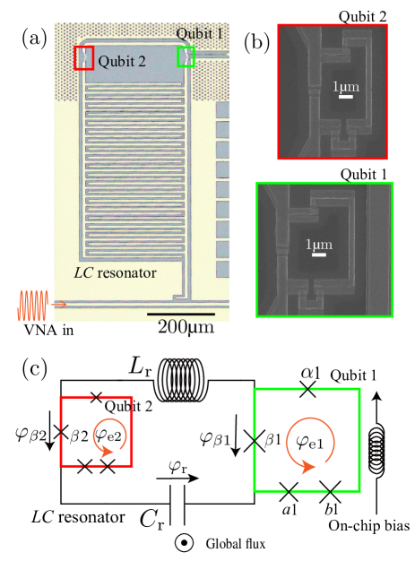
Figure 1: (a) Optical microscope image of the measured sample. The sample holder has a coil to bias a uniform magnetic field from the back surface of the chip. Qubit 1 has a local bias line that changes the magnetic flux of the qubit loop. The spectrum is measured using a vector network analyzer (VNA) for probing and reading from the transmission line shown below the circuit. (b) SEM images of qubits 1 and 2. The design parameters of both qubit junctions are the same. (c) Equivalent circuit diagram of the sample.

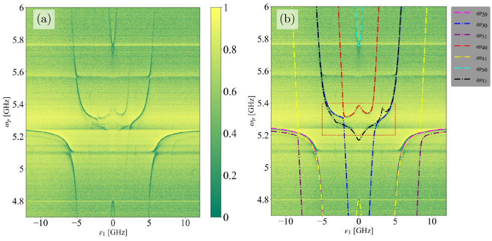
Figure 2: Pump frequency $\omega_{p}$ from the VNA versus the persistent current energy $\varepsilon_{1}$ of qubit 1. (a) Raw data of the observed single-tone spectrum of the sample shown in Fig. 1. (b) Observed single-tone spectrum with fitted curves corresponding to the state transition frequencies $\omega_{ij}$ between the $i$-th and $j$-th eigenstates of Hamiltonian (6). The fit parameters are $g_{1}/2\pi=3.31$, $g_{2}/2\pi=3.41$, $\Delta_{\mathrm{q1}}/2\pi=1.35$, $\Delta_{\mathrm{q2}}/2\pi=1.26$, $\omega_{\mathrm{r}}/2\pi=5.14$, and $\varepsilon_{2}/2\pi=-3.21$ GHz. Note that $\omega_{31}$ and $\omega_{51}$ are not used for fitting because those signals were too weak, but the curves of $\omega_{31}$ and $\omega_{51}$ still reproduce well the experimental results. Around 5.09 GHz and 5.57 GHz can be seen parasitic modes, which originate from, for example, sample ground planes and/or the measurement environment; this includes the sample holder and microwave components coupled to the system.

Device

Figure 1(a) shows an optical microscope image of the artificial-atom–resonator circuit. The $LC$ resonator is composed of an interdigital capacitor and line inductance made of a superconducting thin film [34, 35]. The two flux qubits are inductively coupled to the $LC$ resonator via a Josephson junction [Fig. 1(b)], which increases the couplings to the ultrastrong regime. The energies of the flux qubits [36] can be changed applying an external magnetic flux to the loop from a global coil and using an on-chip bias line. Figure 1(c) shows the equivalent circuit with lumped elements and Josephson junctions.

The Hamiltonian of the entire system is [37, 38, 39]

$$\hat{\mathcal{H}}_{\mathrm{tot}}=\hat{\mathcal{H}}_{\mathrm{q1}}+\hat{\mathcal{H}}_{\mathrm{q2}}+\hat{\mathcal{H}}_{\mathrm{r}}+\hat{\mathcal{H}}_{\mathrm{int}}\,,$$ (1)

where $\hat{\mathcal{H}}_{\mathrm{q}k}$ ($k=1,2$), $\hat{\mathcal{H}}_{\mathrm{r}}$, and $\hat{\mathcal{H}}_{\mathrm{int}}$ represent the qubits, resonator, and atom-resonator plus atom-atom couplings, respectively. The Hamiltonian of the resonator is $\hat{\mathcal{H}}_{\mathrm{r}}=\hbar\omega_{\mathrm{r}}\quantity(\hat{a}^{\dagger}\hat{a}+1/2)$, where $\omega_{\mathrm{r}}\equiv 1/\sqrt{L_{\mathrm{r}}C_{\mathrm{r}}}$ is the resonance frequency, $\hat{a}\equiv(\hat{\phi}_{\mathrm{r}}-iZ_{\mathrm{r}}\hat{q}_{\mathrm{r}})/\sqrt{2\hbar Z_{\mathrm{r}}}$ is the annihilation operator, $\hat{a}^{\dagger}\equiv(\hat{\phi}_{\mathrm{r}}+iZ_{\mathrm{r}}\hat{q}_{\mathrm{r}})/\sqrt{2\hbar Z_{\mathrm{r}}}$ is the creation operator, $Z_{\mathrm{r}}=\sqrt{L_{\mathrm{r}}/C_{\mathrm{r}}}$ is the characteristic impedance of the $LC$ resonator, and $\hat{q}_{\mathrm{r}}$ is the conjugate variable of $\hat{\phi}_{\mathrm{r}}=\Phi_{0}\hat{\varphi}_{\mathrm{r}}$. The Hamiltonian of the $k$-th artificial atom is defined as

$$\hat{\mathcal{H}}_{{\mathrm{q}k}}\equiv 4E_{\mathrm{c}}\hat{\mathbf{q}}_{k}^{\mathrm{T}}\mathbf{M}_{k}^{-1}{\hat{\mathbf{q}}_{k}}+E_{\mathrm{Lr}}\hat{\varphi}_{\beta k}^{2}+\hat{\mathcal{U}}_{\mathrm{J}k}\,,$$ (2)

where $E_{c}$ is the charging energy of the Josephson junction, $\mathbf{M}_{k}$ is the normalized mass matrix, $E_{\mathrm{Lr}}=\Phi_{0}^{2}/(2L_{\mathrm{r}})$, and $\hat{\mathcal{U}}_{\mathrm{J}k}$ is the qubit potential energy of Josephson junctions:

$$\!\!\!\hat{\mathcal{U}}_{\mathrm{J}k}(\hat{\varphi}_{\mathrm{e}k})= \!-\!E_{\mathrm{J}}\!\left[\,\beta_{k}\cos{(\hat{\varphi}_{\beta k})}\!+\!\cos{(\hat{\varphi}_{ak})}\!+\!\cos{(\hat{\varphi}_{bk})}\right.$$

$$\,\,\,\,\left.+\alpha_{k}\cos{(\varphi_{\mathrm{e}k}-\hat{\varphi}_{ak}-\hat{\varphi}_{bk}-\hat{\varphi}_{\beta k})}\right]\,.$$ (3)

Here, $E_{\mathrm{J}}$ is the current energy of the Josephson junction, and $\varphi_{\mathrm{e}k}$ represents the external flux for the loop of each atom. The interaction Hamiltonian

$$\hat{\mathcal{H}}_{\mathrm{int}}=-E_{\mathrm{Lr}}(\hat{\varphi}_{\beta 1}\hat{\varphi}_{\mathrm{r}}-\hat{\varphi}_{\beta 2}\hat{\varphi}_{\mathrm{r}}+\hat{\varphi}_{\beta 1}\hat{\varphi}_{\beta 2})$$ (4)

is obtained from the boundary condition (Kirchhoff’s voltage law) of the loop forming the resonator with elements $L_{\mathrm{r}}$ and $C_{\mathrm{r}}$.

By approximating each atom as a two-level system [40], on the basis of persistent currents of the superconducting loop, we obtain the total Hamiltonian in Eq. (1) as

$$\hat{\mathcal{H}}_{\mathrm{tot}}/\hbar \simeq\omega_{\mathrm{r}}\hat{a}^{\dagger}\hat{a}\!+\!\frac{\varepsilon_{1}}{2}\hat{\sigma}_{z1}\!+\!\frac{\Delta_{1}}{2}\hat{\sigma}_{x1}\!+\!\frac{\varepsilon_{2}}{2}\hat{\sigma}_{z2}\!+\!\frac{\Delta_{2}}{2}\hat{\sigma}_{x2}$$

$$-(g_{1}\hat{\sigma}_{z1}-g_{2}\hat{\sigma}_{z2})(\hat{a}^{\dagger}+\hat{a})-\frac{2g_{1}g_{2}}{\omega_{\mathrm{r}}}\hat{\sigma}_{z1}\hat{\sigma}_{z2}\,,$$ (5)

where $\varepsilon_{k}$ is the persistent current energy of each qubit, $\Delta_{k}$ is the qubit energy gap when $\varepsilon_{k}=0$, while $\hat{\sigma}_{zk}$ and $\hat{\sigma}_{xk}$ are the Pauli matrices for the $k$-th qubit. We define $\varepsilon_{k}>0$ when the qubit current flows anticlockwise and vice versa.

After a unitary transformation that diagonalizes the atomic Hamiltonians $\hat{\mathcal{H}}_{\mathrm{qk}}$, we obtain a generalized Dicke Hamiltonian [41] with the spin-spin interaction:

$$\hat{\mathcal{H}}_{\mathrm{tot}}/\hbar\simeq\omega_{\mathrm{r}}\hat{a}^{\dagger}\hat{a}+\frac{\omega_{\mathrm{q1}}}{2}\hat{\sigma}_{z1}+\frac{\omega_{\mathrm{q2}}}{2} \hat{\sigma}_{z2}$$

$$-(g_{1}\hat{\Lambda}_{1}-g_{2}\hat{\Lambda}_{2})(\hat{a}^{\dagger}+\hat{a}) -\frac{2g_{1}g_{2}}{\omega_{\mathrm{r}}}\hat{\Lambda}_{1}\hat{\Lambda}_{2}\,,$$ (6)

where $\omega_{\mathrm{q}k}={\rm sgn}(\varepsilon_{k})(\varepsilon_{k}^{2}+\Delta_{k}^{2})^{1/2}$ is the qubit frequency and $\hat{\Lambda}_{k}=(\cos{\theta_{k}}\,\hat{\sigma}_{xk}+\sin{\theta_{k}}\,\hat{\sigma}_{zk})$ gives the direction of the interaction, with $\theta_{k}\simeq-\arctan(\Delta_{k}/\varepsilon_{k})$ (details in Appendix A). For $\theta_{k}=0$ $(\varepsilon_{k}=0)$ the interaction is transverse. When $\theta_{k}\neq 0$, the interaction has a longitudinal component and the one photon exciting two atoms effect is allowed.

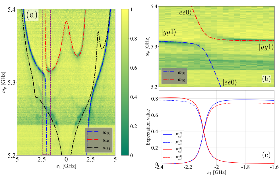
Figure 3: (a) Enlarged view of the central part of the spectrum in Fig. 2(b) with fitting curve. The fitting reproduces the spectrum well. (b) Enlarged image of the anticrossing between $\omega_{30}$ and $\omega_{40}$. (c) Projection of $\ket{gg1}$ and $\ket{ee0}$ bare states to the third and fourth eigenstates calculated using the fitting parameters and Hamiltonian in Eq. (6).

Results

Energy spectrum

Figure 2(a) shows the raw data of the measured spectrum as a function of the persistent current energy $\varepsilon_{1}$ of qubit 1, after fixing the value of $\varepsilon_{2}/2\pi$ at $-3.21$ GHz when $\varepsilon_{1}=0$. In Fig. 2(b) the spectrum is fitted with the numerically calculated transition frequencies $\omega_{ij}$ between the $i$-th and $j$-th eigenstates of the total Hamiltonian $\hat{\mathcal{H}}_{\mathrm{tot}}$. The persistent current energy for qubit 2 and the resonator frequency are affected by the external magnetic flux applied to qubit 1 [8]. Thus, to derive the transitions frequencies $\omega_{ij}$, in Eq. (5), we substitute $\varepsilon_{2}\xrightarrow{}\varepsilon_{2}+A\varepsilon_{1}$ and $\omega_{\mathrm{r}}\xrightarrow{}\omega_{\mathrm{r}}(1+B_{\pm}\varepsilon_{1})$, where $A$ and $B_{\pm}$ are fitting parameters. Because the spectrum is asymmetric with respect to the sign of $\varepsilon_{1}$, we use two different values for $B_{\pm}$, where $B_{+}$ is used when $\varepsilon_{1}\geq 0$ and vice versa. From the fitting, we obtain $A=-9.10\times 10^{-3}$, $B_{-}=1.13\times 10^{-3}$, and $B_{+}=0.79\times 10^{-3}$. To calculate the spectrum, we used the quantum toolbox in Python (QuTip) [42, 43].

Flux qubits 1 and 2 are almost identical except for the loop size; consequently, they have similar fitted parameters, i.e., $\Delta_{\mathrm{q1}}=0.26\,\omega_{\mathrm{r}}$ and $\Delta_{\mathrm{q2}}=0.25\,\omega_{\mathrm{r}}$. We find atom-resonator couplings rates of $g_{1}/\omega_{\mathrm{r}}=0.64$ and $g_{2}/\omega_{\mathrm{r}}=0.66$, indicating that the artificial atoms are ultrastrongly coupled with the resonator.

Observing $\omega_{30}$ (blue curve) and $\omega_{40}$ (red curve) in Figs. 2(b) and especially 3(a), it is possible to notice that the spectrum is asymmetric with respect to the sign of $\varepsilon_{1}$. This occurs due to the presence of atom-light longitudinal interactions when two or more qubits are coupled to the same cavity mode [44]. Assuming that there are only longitudinal couplings, the atomic states are associated to photonic coherent states. However, if $\varepsilon_{1}>0$, the atomic and photonic states are decoupled if $M=m_{1}-m_{2}=0$, where $m_{k}=\pm 1$ is the eigenstate of $\sigma_{zk}$ (details in Appendix B). If $\varepsilon_{1}<0$, the atomic and photonic states are decoupled if $M=-m_{1}-m_{2}=0$. In our experimental setup we have both longitudinal and transverse couplings; the presence of the longitudinal components justifies the asymmetry in Fig. 2.

One photon simultaneously excites two atoms

We indicate with $\ket{\psi_{i}}$ the eigenstate of the system Hamiltonian $\hat{\mathcal{H}}_{\mathrm{tot}}$ with eigenenergies $\hbar\omega_{i0}$. The terms $\omega_{\mathrm{q}i}\hat{\sigma}_{zi}/2$ in Eq. (6) define the ground $\ket{g}$ and excited $\ket{e}$ atomic bare states.

In Fig. 3(a), which is an enlarged view of the red dashed rectangle in Fig. 2(b), the white arrow indicates the anticrossing between the eigenstates $\ket{\psi_{3}}$ and $\ket{\psi_{4}}$, with eigenfrequencies $\omega_{30}$ and $\omega_{40}$. In correspondence of the anticrossing [see Fig. 3(b)], we numerically calculate the projection $P_{j}^{(i)}\equiv\absolutevalue{\innerproduct{\psi_{i}}{j}}^{2}$ of the third and fourth eigenstates $\ket{\psi_{i}}$ $(i=3,4)$ on the bare states $\ket{j}=\{\ket{gg1},\ket{ee0}\}$ as a function of $\varepsilon_{1}$. Figure 3(c) shows that, at the anticrossing, the third and fourth eigenstates are approximate symmetric and asymmetric superpositions of $\ket{gg1}$ and $\ket{ee0}$. Considering also that the sum of the bare qubit frequencies are nearly equal to the bare resonator frequency, $\omega_{\mathrm{q1}}+\omega_{\mathrm{q2}}\simeq\omega_{\mathrm{r}}$, the anticrossing is the signature of the one photon exciting two atoms effect. Half of the minimum split between $\omega_{30}$ and $\omega_{40}$ in the spectrum gives the effective coupling between $\ket{gg1}$ and $\ket{ee0}$, that is 22 MHz (details in Appendix C).

With respect to the theoretical prediction in Ref. 30, our system has a much larger coupling. This implies that the system eigenstates should have a strong dressing, and in principle we could not observe a clean one photon exciting two atoms effect. However, the spin-spin interaction, that is not considered in Ref. 30, reduces the dressing. When $\varepsilon_{1}$ and $\varepsilon_{2}$ are both negative, the system states are decoupled with respect to the longitudinal interaction if $M=m_{1}-m_{2}=0$. This occurs when $m_{1}=m_{2}=\pm 1$, so when the atoms are both either in the ground $\ket{gg}$ or in the excited $\ket{ee}$ states. However, the transverse interactions still affect our system generating a small dressing that reduces the projection $P_{gg1}^{(4)}$ and $P_{ee0}^{(3)}$ to almost $0.8$ at $\varepsilon_{1}/2\pi=-2.4$ GHz.

Discussion

We measured the spectrum of a circuit composed of two artificial atoms ultrastrongly coupled to a $LC$ resonator. The generalized Dicke Hamiltonian with spin-spin interaction describes well the measured spectrum. At the energy where the sum of the atomic energies almost matches the one of the resonator, we observed one anticrossing between the states $\ket{gg1}$ and $\ket{ee0}$. This experimentally confirms the recent theoretical prediction that one-photon can simultaneously excites two atoms  [30], opening a new chapter in quantum nonlinear optics.

Future work would involve reading out the qubit and photon states [45] as well as observing the one photon exciting two atoms dynamics. These studies could also be extended to explore, for example, photon down- and up-conversion [29] and ultrafast two qubit gates [14, 17].

Data availability

The data that support the findings of this study are available from the corresponding authors upon reasonable request.

Author contributions

A.T. designed the device, carried out the experiment and analyzed the data. A.T. and R.S. performed theoretical and numerical calculations. H.M. carried out part of the experiment. All the authors participated in the discussions and wrote and contributed to editing the manuscript.

Appendix Appendix A Circuit Hamiltonian

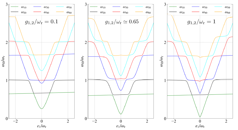
Figure A1: Frequency difference $\omega_{i0}$ for the lowest-energy eigenstates of Hamiltonian Eq. (C36) using different coupling ratio $g_{1,2}/\omega_{\mathrm{r}}\simeq 0$, 0.65 (fitted value), and 1. Other parameters for Eq. (C36) are obtained from fitting the spectrum Fig. 2 The tilt in the horizontal axis originates from the fitting parameter $A$ caused mainly by crosstalk.

Here we describe the circuit Hamiltonian calculation in detail. The branch fluxes across the circuit elements, which are junctions, the inductance $L_{\mathrm{r}}$, and the capacitance $C_{\mathrm{r}}$, follow Kirchhoff’s voltage laws:

$$\varphi_{\beta 1}+\varphi_{\alpha 1}+\varphi_{a1}+\varphi_{b1}=\varphi_{\mathrm{e}1}\,,$$ (A1)

$$\varphi_{\beta 2}+\varphi_{\alpha 2}+\varphi_{a2}+\varphi_{b2}=\varphi_{\mathrm{e}2}\,,$$ (A2)

$$\varphi_{\mathrm{cr}}+\varphi_{\mathrm{\ell r}}+\varphi_{\beta 1}-\varphi_{\beta 2}=0\,,$$ (A3)

where $\varphi_{\mathrm{cr}}$ and $\varphi_{\mathrm{\ell r}}$ represent fluxes between the resonator capacitor and the inductor. The total Lagrangian of the circuit is described as the summation of circuit components as

$$\mathcal{L}_{\mathrm{tot}}=\mathcal{K}_{\mathrm{J1}}+\mathcal{K}_{\mathrm{J2}}-\mathcal{U}_{\mathrm{J1}}-\mathcal{U}_{\mathrm{J2}}+\mathcal{L}_{\mathrm{r}}\,,$$ (A4)

where

$$\mathcal{K}_{\mathrm{J}k} =\frac{C_{\mathrm{J}}}{2}\left[\,\beta\dot{\phi}_{\beta k}^{2}+\dot{\phi}_{ak}^{2}+\dot{\phi}_{bk}^{2}\right.$$

$$\quad\quad\quad\quad\left.+\alpha_{i}(\dot{\phi}_{\beta k}+\dot{\phi}_{ak}+\dot{\phi}_{bk})^{2}\right]\,,$$ (A5)

$$\begin{split}\mathcal{U}_{\mathrm{J}k}=-E_{\mathrm{J}}&\left[\beta_{i}\cos(\varphi_{\beta k})+\cos{(\varphi_{ak})}+\cos{(\varphi_{bk})}\right.\\ &\left.+\alpha_{i}\cos{(\varphi_{\mathrm{e}k}-\varphi_{\beta k}-\varphi_{ak}-\varphi_{bk})}\right]\,,\end{split}$$ (A6)

$$\mathcal{L}_{\mathrm{r}}=\frac{C_{\mathrm{r}}}{2}\dot{\phi}_{\mathrm{cr}}^{2}-\frac{1}{2L_{\mathrm{r}}}(\phi_{\mathrm{cr}}+\phi_{\beta 1}-\phi_{\beta 2})^{2}\,,$$ (A7)

and $k\in\{1,2\}$ represents the index of a qubit. The sub-index $cr$ refers to the capacitor of the resonator. The qubit kinetic energy part of the Lagrangian in Eq. (A4) becomes

$$\mathcal{K}_{\mathrm{J}i}=\frac{1}{2}\dot{\boldsymbol{\upphi}}{\!}^{\mathrm{T}}\mathbf{M}\dot{\boldsymbol{\upphi}}\,,$$ (A8)

where $\boldsymbol{\upphi}_{k}\equiv\matrixquantity(\phi_{\beta k}&\phi_{ak}&\phi_{bk})^{\mathrm{T}}$ and the mass matrix is given by

Using the canonical conjugate $q_{i}=\partial\mathcal{}{L}_{\mathrm{tot}}/\partial\dot{\phi}_{i}$ for $\dot{\phi}_{i}$, where $i\in\{\beta_{k},a_{k},b_{k}\}$, we can rewrite Eq. (A8) as

$$\mathcal{K}_{\mathrm{J}k}=\frac{1}{2}\mathbf{q}_{k}^{\mathrm{T}}\mathbf{M}^{-1}\mathbf{q}_{k}\,.$$ (A9)

Then, we obtain the total Hamiltonian of the circuit as

$$\mathcal{H}_{\mathrm{tot}} =\sum_{k}\mathbf{q}_{k}^{\mathrm{T}}\dot{\boldsymbol{\upphi}}_{k}-\mathcal{L}_{\mathrm{tot}}$$

$$=\sum_{k}(4E_{\mathrm{c}}\tilde{\mathbf{q}}_{k}^{\mathrm{T}}\tilde{\mathbf{M}}_{k}^{-1}\tilde{\mathbf{q}}_{k}+E_{\mathrm{Lr}}\varphi_{\beta k}^{2}+\mathcal{U}_{\mathrm{J}k})$$

$$\quad\,\,\,+\mathcal{H}_{\mathrm{r}}+\mathcal{H}_{\mathrm{int}}\,,$$ (A10)

where $2e\tilde{q}=q$ and $C_{\mathrm{J}}\tilde{\mathbf{M}}=\mathbf{M}$, and the term $E_{\mathrm{Lr}}\varphi_{\beta k}$ originates from Eq. (A7) because we define

$$\mathcal{H}_{\mathrm{r}}\equiv\frac{C_{\mathrm{r}}}{2}\dot{\phi}_{\mathrm{cr}}^{2}+\frac{1}{2L_{\mathrm{r}}}\phi_{\mathrm{cr}}^{2}\,,$$ (A11)

as a bare $LC$ resonator. We expand the total Hamiltonian Eq. (A10) using the eigenvectors $\ket{i}_{k}$ (${i}\in\mathbb{N}$) of the atom Hamiltonians ($\mathcal{H}_{\mathrm{tot}}-\mathcal{H}_{\mathrm{r}}-\mathcal{H}_{\mathrm{int}}$),

$$\!\!\!\hat{\mathcal{H}}_{\mathrm{tot}}= \hbar\sum_{i}{(\Omega_{i}^{(1)}\ket{i}_{1}\bra{i}_{1}+\Omega_{i}^{(2)}\ket{i}_{2}\bra{i}_{2})}+\hat{\mathcal{H}}_{\mathrm{r}}$$

$$\!\!-\hbar\sum_{i,j}{(g_{ij}^{(1)}\ket{i}_{1}\bra{j}_{1}\!\!-g_{ij}^{(2)}\ket{i}_{2}\bra{j}_{2})(\hat{a}^{\dagger}\!+\hat{a})}$$

$$-E_{\mathrm{L}}\sum_{i,j}{g_{ij}^{(1)}g_{ij}^{(2)}\ket{i}_{1}\ket{i}_{2}\bra{j}_{1}\bra{j}_{2}}\,,$$ (A12)

where $\hbar\Omega_{i}^{(k)}$ is the $i$-th eigenenergy of atom $k$ and $\hbar g_{ij}^{(k)}=I_{\mathrm{zpf}}\Phi_{0}\matrixelement{i}{\hat{\varphi}_{\beta k}}{j}$ is the coupling matrix element ($I_{\mathrm{zpf}}=\sqrt{\hbar\omega_{\mathrm{r}}/2L_{\mathrm{r}}}$). When we use the two lowest eigenstates for each qubit, we can obtain the Hamiltonian with the two-level system qubits and the $N$-level system resonator as shown in Eqs. (5) and (6). In Eqs. (5) and (6), the spin-spin interaction reduces the current flowing in the resonator loop, which in this system is the ferromagnetic coupling.

For the fitting, we use Eq. (6), and 11 fitting parameters, this includes the offset value when $\varepsilon_{1}=0$ and the persistent current $I_{\mathrm{p1}}$ in qubit 1 to derive $\varepsilon_{1}=I_{\mathrm{p1}}\Phi_{0}(\varphi_{\mathrm{e1}}-0.5)$, where $\Phi_{0}$ is the flux quantum. We also use the photo-processing technique to obtain peak points from the spectrum [46, 47, 37].

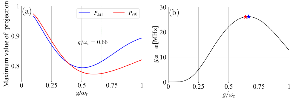
Figure A2: The left panel shows the maximum value of the projections $P_{gg1}(g/\omega_{\mathrm{r}})$ and $P_{ee0}(g/\omega_{\mathrm{r}})$ at the antisplitting point. The green dotted vertical line corresponds to the value that maximizes $g_{30-40}$. the right panel shows the effective coupling constant $g_{30-40}$ plotted against the coupling ratio $g/\omega_{\mathrm{r}}$. The red and blue star represent $g_{1}/\omega_{\mathrm{r}}=0.64$ and $g_{2}/\omega_{\mathrm{r}}=0.67$, respectively.

Appendix Appendix B Asymmetric spectrum in the generalized Dicke Hamiltonian

Consider the system Hamiltonian [Eq. (6)] with $\Delta_{k}=0$, $g_{1}=g_{2}=g$, and substituting $\sigma_{zk}$ with its eigenvalue $m_{k}=\pm 1$, we can write:

$$\mathcal{H}_{s}/\hbar=\frac{|\varepsilon_{1}|}{2}m_{1}+\frac{|\varepsilon_{2}|}{2}m_{2}+\omega_{\mathrm{r}}a^{\dagger}a+gM(a^{\dagger}+a)\,,$$ (B13)

with $M={\rm sgn}(\varepsilon_{2})m_{2}-{\rm sgn}(\varepsilon_{1})m_{1}$. Performing the substitution $\hat{a}=\hat{b}-Mg/\omega_{\mathrm{r}}$ in Eq. C39,

$$\mathcal{H}_{s}/\hbar =\frac{|\varepsilon_{1}|}{2}m_{1}+\frac{|\varepsilon_{2}|}{2}m_{2}$$

$$\quad\quad+\omega_{\mathrm{r}}(\hat{b}^{\dagger}-M\frac{g}{\omega_{\mathrm{r}}})(\hat{b}-M\frac{g}{\omega_{\mathrm{r}}})$$

$$\quad\quad+gM(\hat{b}^{\dagger}-M\frac{g}{\omega_{\mathrm{r}}}+\hat{b}-M\frac{g}{\omega_{\mathrm{r}}})\,,$$ (B14)

$$=\omega_{\mathrm{r}}b^{\dagger}b+\frac{|\varepsilon_{1}|}{2}m_{1}+\frac{|\varepsilon_{2}|}{2}m_{2}-M^{2}\frac{g^{2}}{\omega_{\mathrm{r}}}\,,$$ (B15)

we obtain the Hamiltonian of a harmonic oscillator. By applying the annihilation operator $\hat{b}$ to its ground state $\ket{0}_{M}$ (i.e. $\hat{b}\ket{0}_{M}=0$), we thus obtain

$$\hat{a}\ket{0}_{M}=-M\frac{g}{\omega_{\mathrm{r}}}\ket{0}_{M}\,.$$ (B16)

From Eq. B16, we see that atomic states with $M=0$ are associated with the zero-photon state; while atomic states with $M=\pm 2$ are associated with the photonic coherent states $\ket{\pm\alpha}$. In turn, $M$ depends on the sign of $\varepsilon_{1}$ and $\varepsilon_{2}$. If $\varepsilon_{1}<0$ and $\varepsilon_{2}<0$, then $M_{-}\equiv M=m_{1}-m_{2}$. If $\varepsilon_{1}>0$ and $\varepsilon_{2}<0$, then $M_{+}\equiv M=-(m_{1}+m_{2})$. Table LABEL:t1 shows the eight possible states as a function of the sign of $\varepsilon_{1}$ when the interaction is longitudinal. This explains the asymmetry of the spectra respect the sign of $\varepsilon_{1}$.

Table 1: Possible values of $M$ and relative states. We consider $\varepsilon_{2}<0$.

$m_{1}$	-1	+1	-1	+1
$m_{2}$	-1	-1	+1	+1
$M_{-}$	0	+2	-2	0
States if $\varepsilon_{1}<0$	$\ket{gg}\ket{0}$	$\ket{eg}\ket{-\alpha}$	$\ket{ge}\ket{+\alpha}$	$\ket{ee}\ket{0}$
$M_{+}$	+2	0	0	-2
States if $\varepsilon_{1}>0$	$\ket{gg}\ket{+\alpha}$	$\ket{eg}\ket{0}$	$\ket{ge}\ket{0}$	$\ket{ee}\ket{-\alpha}$

Appendix Appendix C Coupling ratio dependence of one photon exciting two atoms

Figure A1 shows the numerically calculated transition frequency $\omega_{i0}$ (spectrum) for the coupling ratios $g_{1,2}/\omega_{\mathrm{r}}=0$, 0.65 (fitted value), and 1. We use the same Hamiltonian in Eq. (6),

$$\hat{\mathcal{H}}_{\mathrm{tot}}/\hbar\simeq \omega_{\mathrm{r}}\hat{a}^{\dagger}\hat{a}$$

$$\!+\frac{\varepsilon_{1}}{2}\hat{\sigma}_{z1}+\frac{\Delta_{1}}{2}\hat{\sigma}_{x1}+\frac{\varepsilon_{2}}{2}\hat{\sigma}_{z2}+\frac{\Delta_{2}}{2}\hat{\sigma}_{x2}$$

$$\!-(g_{1}\hat{\sigma}_{z1}\!-\!g_{2}\hat{\sigma}_{z2})(\hat{a}^{\dagger}\!+\hat{a})\!-\!\frac{2g_{1}g_{2}}{\omega_{\mathrm{r}}}\hat{\sigma}_{z1}\hat{\sigma}_{z2}\,,$$ (C36)

and fitting parameters. We can see that the asymmetry of the spectrum increases with $g_{1,2}/\omega_{\mathrm{r}}$, and the antisplitting gap between $\omega_{30}$ and $\omega_{40}$ in $g_{1,2}/\omega_{\mathrm{r}}\simeq 0.65$ ($-1<\varepsilon_{1}/\omega_{\mathrm{r}}<0$) is larger than that of the other two coupling ratios.

We numerically calculate the projection $P_{j}\equiv\absolutevalue{\innerproduct{\Psi_{j}}{j}}^{2}$ of the superposition states,

$$\ket{\Psi_{gg1}}\simeq(\ket{\psi_{3}}+\ket{\psi_{4}})/\sqrt{2}\,(\simeq\ket{gg1})\,,$$ (C37)

$$\ket{\Psi_{ee0}}\simeq(\ket{\psi_{3}}-\ket{\psi_{4}})/\sqrt{2}\,(\simeq\ket{ee0})\,,$$ (C38)

at the anticrossing point on the bare states $\ket{j}=\{\ket{gg1},\ket{ee0}\}$ as a function of the coupling ratio, and the result is shown in Fig. A2(a). As mentioned in the theoretical prediction in Ref. 30, a lower $g/\omega_{\mathrm{r}}$ maximizes the projection. However, the effective coupling strength below $g/\omega_{\mathrm{r}}=0.1$ is much smaller than that at larger coupling ratios, see Fig. A2(b). Thus, when $g/\omega_{\mathrm{r}}$ is below 0.1, we cannot clearly see the antisplitting between $\ket{gg1}$ and $\ket{ee0}$ and the one photon exciting two atoms effect. As shown in the right panel of Fig. A2, the effective coupling is maximum at around $g_{1,2}/\omega_{\mathrm{r}}\simeq 0.66$, which is close to our system.

According to the theoretical prediction in Ref. 30, when the Hamiltonian has no direct spin-spin interaction, which is written as

$$\mathcal{H}_{\mathrm{ideal}}/\hbar= \frac{\omega_{\mathrm{q}}}{2}\sum_{i=1,2}{\hat{\sigma}_{zi}}+\omega_{\mathrm{r}}a^{\dagger}a$$

$$+g\sum_{i=1,2}(\hat{\sigma}_{zi}\cos{\theta}+\hat{\sigma}_{xi}\sin{\theta})(\hat{a}^{\dagger}+\hat{a})\,,$$ (C39)

the effective coupling strength $\Omega$ between $\ket{gg1}$ and $\ket{ee0}$ can be approximate to

$$\Omega\simeq\frac{8}{3}\frac{g^{3}}{\omega_{\mathrm{q}}^{2}}\sin{\theta}\cos{\theta}^{2}\,,$$ (C40)

where $\omega_{\mathrm{q}}$ is the qubit frequency, and $\theta=\arctan(-\Delta/\varepsilon)$. The parameters in our system are $\theta_{1}\simeq 0.09\times 2\pi$, $\theta_{2}\simeq 0.06\times 2\pi$, $\omega_{\mathrm{q1}}\simeq 3.42$ GHz, and $\omega_{\mathrm{q2}}\simeq 2.48$ GHz. From Eq. (C40), the effective coupling constant $\Omega$ obtained using the parameters in our system is expected to be more than 200 MHz. The measured effective coupling constant $g_{30-40}$ is much suppressed. Besides, if the Hamiltonian has no direct spin-spin interaction, the projections on $\ket{gg1}$ and $\ket{ee0}$ at the anticrossing point is less than 0.8 when $g/\omega_{\mathrm{r}}=0.25$, and when $g/\omega_{\mathrm{r}}\gg 0.25$, the one photon exciting two atoms effect is no longer observed.

References

- Nakamura et al. [1999] Y. Nakamura et al., Coherent control of macroscopic quantum states in a single-Cooper-pair box, Nature 398, 786 (1999).
- Gu et al. [2017] X. Gu et al., Microwave photonics with superconducting quantum circuits, Physics Reports 718-719, 1 (2017).
- Krantz et al. [2019] P. Krantz et al., A quantum engineer’s guide to superconducting qubits, Applied Physics Reviews 6, 021318 (2019).
- Kjaergaard et al. [2020] M. Kjaergaard et al., Superconducting Qubits: Current State of Play, Annual Review of Condensed Matter Physics 11, 369 (2020).
- Blais et al. [2021] A. Blais et al., Circuit quantum electrodynamics, Reviews of Modern Physics 93, 025005 (2021).
- Kwon et al. [2021] S. Kwon et al., Gate-based superconducting quantum computing, Journal of Applied Physics 129, 041102 (2021).
- Niemczyk et al. [2010] T. Niemczyk et al., Circuit quantum electrodynamics in the ultrastrong-coupling regime, Nature Physics 6, 772 (2010).
- Yoshihara et al. [2017] F. Yoshihara et al., Superconducting qubit–oscillator circuit beyond the ultrastrong-coupling regime, Nature Physics 13, 44 (2017).
- Forn-Díaz et al. [2017] P. Forn-Díaz et al., Ultrastrong coupling of a single artificial atom to an electromagnetic continuum in the nonperturbative regime, Nature Physics 13, 39 (2017).
- Bosman et al. [2017] S. J. Bosman et al., Multi-mode ultra-strong coupling in circuit quantum electrodynamics, npj Quantum Information 3, 1 (2017).
- Ao et al. [2023] Z. Ao et al., Extremely large Lamb shift in a deep-strongly coupled circuit QED system with a multimode resonator, Scientific Reports 13, 11340 (2023).
- Frisk Kockum et al. [2019] A. Frisk Kockum et al., Ultrastrong coupling between light and matter, Nature Reviews Physics 1, 19 (2019).
- Forn-Díaz et al. [2019] P. Forn-Díaz et al., Ultrastrong coupling regimes of light-matter interaction, Reviews of Modern Physics 91, 025005 (2019).
- Romero et al. [2012] G. Romero et al., Ultrafast Quantum Gates in Circuit QED, Physical Review Letters 108, 120501 (2012).
- Kyaw et al. [2015] T. H. Kyaw et al., Creation of quantum error correcting codes in the ultrastrong coupling regime, Physical Review B 91, 064503 (2015).
- Wang et al. [2016] Y. Wang et al., Holonomic quantum computation in the ultrastrong-coupling regime of circuit QED, Physical Review A. 94, 012328 (2016).
- Wang et al. [2017] Y. Wang et al., Ultrafast quantum computation in ultrastrongly coupled circuit QED systems, Scientific Reports 7, 44251 (2017).
- Stassi et al. [2020] R. Stassi et al., Scalable quantum computer with superconducting circuits in the ultrastrong coupling regime, npj Quantum Information 6, 1 (2020).
- Chen et al. [2021] Y.-H. Chen et al., Fast binomial-code holonomic quantum computation with ultrastrong light-matter coupling, Physical Review Research 3, 033275 (2021).
- [20] S. D. Liberato et al., Quantum vacuum radiation spectra from a semiconductor microcavity with a time-modulated vacuum Rabi frequency, Physical Review Letters 98, 103602.
- Ashhab and Nori [2010] S. Ashhab and F. Nori, Qubit-oscillator systems in the ultrastrong-coupling regime and their potential for preparing nonclassical states, Physcal Review A 81, 042311 (2010).
- Stassi et al. [2013] R. Stassi et al., Spontaneous Conversion from Virtual to Real Photons in the Ultrastrong-Coupling Regime, Physical Review Letters 110, 243601 (2013).
- Cirio et al. [2016] M. Cirio et al., Ground State Electroluminescence, Physical Review Letters 116, 113601 (2016).
- Stassi et al. [2023] R. Stassi et al., Unveiling and veiling an entangled light-matter quantum state from the vacuum, Physical Review Research 5, 043095 (2023).
- Wang et al. [2023] S.-P. Wang et al., Probing the symmetry breaking of a light–matter system by an ancillary qubit, Nature Communications 14, 4397 (2023).
- Garziano et al. [2014] L. Garziano et al., Vacuum-induced symmetry breaking in a superconducting quantum circuit, Physical Review A 90, 043817 (2014).
- Garziano et al. [2015] L. Garziano et al., Multiphoton quantum Rabi oscillations in ultrastrong cavity QED, Physical Review A 92, 063830 (2015).
- Stassi et al. [2017] R. Stassi et al., Quantum nonlinear optics without photons, Physical Review A 96, 023818 (2017).
- Kockum et al. [2017] A. F. Kockum et al., Deterministic quantum nonlinear optics with single atoms and virtual photons, Physical Review A 95, 063849 (2017).
- Garziano et al. [2016] L. Garziano et al., One Photon Can Simultaneously Excite Two or More Atoms, Physical Review Letters 117, 043601 (2016).
- Ball [2016] P. Ball, Two Atoms Can Jointly Absorb One Photon, Physics 9, 83 (2016).
- So et al. [2000] P. T. C. So et al., Two-photon excitation fluorescence microscopy, Annual Review of Biomedical Engineering 2, 399 (2000).
- Denk et al. [1990] W. Denk et al., Two-Photon Laser Scanning Fluorescence Microscopy, Science 248, 73 (1990).
- Miyanaga et al. [2021] T. Miyanaga et al., Ultrastrong Tunable Coupler Between Superconducting Resonators, Physical Review Applied 16, 064041 (2021).
- Zotova et al. [2023] J. Zotova et al., Compact Superconducting Microwave Resonators Based on Capacitors, Physical Review Applied 19, 044067 (2023).
- Chiorescu et al. [2004] I. Chiorescu et al., Coherent dynamics of a flux qubit coupled to a harmonic oscillator, Nature 431, 159 (2004).
- Tomonaga et al. [2021] A. Tomonaga et al., Quasiparticle tunneling and charge noise in ultrastrongly coupled superconducting qubit and resonator, Physical Review B 104, 224509 (2021).
- Billangeon et al. [2015] P.-M. Billangeon et al., Circuit-QED-based scalable architectures for quantum information processing with superconducting qubits, Physical Review B 91, 094517 (2015).
- Robertson et al. [2006] T. L. Robertson et al., Quantum theory of three-junction flux qubit with non-negligible loop inductance: Towards scalability, Physcal Review B 73, 174526 (2006).
- Yoshihara et al. [2022] F. Yoshihara et al., Hamiltonian of a flux qubit-LC oscillator circuit in the deep–strong-coupling regime, Scientific Reports 12, 6764 (2022).
- Du et al. [2012] L.-H. Du et al., Generalized Rabi model in quantum-information processing including the term, Physcal Review A 86, 014303 (2012).
- Johansson et al. [2012] J. R. Johansson et al., QuTiP: An open-source python framework for the dynamics of open quantum systems, Computer Physics Communications 183, 1760 (2012).
- Johansson et al. [2013] J. R. Johansson et al., QuTiP 2: A python framework for the dynamics of open quantum systems, Computer Physics Communications 184, 1234 (2013).
- Jaako et al. [2016] T. Jaako et al., Ultrastrong-coupling phenomena beyond the Dicke model, Physical Review A 94, 033850 (2016).
- Felicetti et al. [2015] S. Felicetti et al., Parity-dependent State Engineering and Tomography in the ultrastrong coupling regime, Scientific Reports 5, 11818 (2015).
- Sato et al. [1998] Y. Sato et al., Three-dimensional multi-scale line filter for segmentation and visualization of curvilinear structures in medical images, Medical Image Analysis 2, 143 (1998).
- Walt et al. [2014] S. v. d. Walt et al., scikit-image: image processing in Python, PeerJ 2, e453 (2014).
Acknowledgements
We thank Y. Zhou, R. Wang, and S. Kwon for their thoughtful comments on this research. This paper was based on results obtained from JSPS KAKENHI (Grant Number JP 22K21294) and a project, JPNP16007, commissioned by the New Energy and Industrial Technology Development Organization (NEDO), Japan. Supporting from JST CREST (Grant No. JPMJCR1676) and Moonshot R&D (Grant No. JPMJMS2067) is also appreciated. R.S. acknowledges the Army Research Office (ARO) (Grant No. W911NF1910065). F.N. is supported in part by: Nippon Telegraph and Telephone Corporation (NTT) Research, the Japan Science and Technology Agency (JST) [via the Quantum Leap Flagship Program (Q-LEAP), and the Moonshot R&D Grant Number JPMJMS2061], the Asian Office of Aerospace Research and Development (AOARD) (via Grant No. FA2386-20-1-4069), and the office of Naval Research (ONR).