Relativistic Covariance of Scattering

Abstract

We analyze relativistic quantum scattering in the Schrödinger picture. The suggestive requirement of translational invariance and conservation of the four-momentum, that the interacting Hamiltonian commute with the four-momentum $P$ of free particles, is shown to imply the absence of interactions.

The relaxed requirement, that the interacting Hamiltonian $H^{\prime}$ commute with the four-velocity $U=P/M$, $M=\sqrt{P^{2}}$, allows Poincaré covariant interactions just as in the nonrelativistic case. If the $S$-matrix is Lorentz invariant, it still commutes with the four-momentum $P$ though $H^{\prime}$ does not.

Shifted observers, whose translations are generated by the four-velocity $U$, just see a shifted superposition of near-mass-degenerate states with unchanged relative phases, while the four-momentum generates oscillated superpositions with changed relative phases.

1 Introduction

Despite the phenomenal agreement of the standard model with observed physics, the mathematical existence of relativistic scattering is still unknown.

In the quantum case and in the classical case relativistic scattering seems excluded by Haag’s [3] and Leutwyler’s [5] no-go theorems.

In textbooks [13] one finds requirements for an interacting representation of Lorentz transformations but not their solution nor any proof of existence.

Assuming that one can switch on the interaction with a function $g:\mathbb{R}^{4}\mapsto[0,1]$, such that $g(x)=0$ in a neighbourhood of $x$ means no interaction and $g(x)=1$ fully switched on interaction, and that the $S$-matrix is a series in $g$, Bogoliubov [1] shows that each unitary, perturbative, relativistic and causal $S$-matrix is the time ordered exponential

$$S[g]=\operatorname{T}\exp{\,\mathrm{i}\!\int\!\operatorname{d}^{\,4}\!\!x\,\mathscr{L}_{\text{int}}(x,g(x))}\ ,$$ (1)

where at each point $x$ the time ordered interaction Lagrangian $\operatorname{T}\mathscr{L}_{\text{int}}(x,g(x))$ is a hermitian, scalar operator which depends on the intensity function $g$ and which is local

$$\phantom{\,}[\operatorname{T}\mathscr{L}_{\text{int}}(x,g(x)),\operatorname{T}\mathscr{L}_{\text{int}}(y,g(y))]=0\text{\qquad if $x-y$ is spacelike}\ .$$ (2)

In the standard model $\operatorname{T}\mathscr{L}_{\text{int}}(x)$ is a normal ordered polynomial in the free fields at $x$ which create and annihilate the elementary particles. But despite its fundamental role the convergence of the series is unknown as is the mathematical existence of relativistic scattering.

Mathematically well defined references on scattering theory [10] restrict their discussion to nonrelativistic scattering and specialize mainly to scattering by potentials which depend on the distance of the two incident particles. Such an interaction is manifestly invariant under Galilei transformations, which govern nonrelativistic motion.

Using the Schrödinger picture we recapitulate the analysis of Reed and Simon in the relativistic case and find that the innocent looking requirement of translational invariance, that the interacting Hamiltonian $H^{\prime}$ commute with the generators $P^{m}$ of the translations of free particles, implies $H^{\prime}=H$ and excludes scattering.

Each representation of the Poincaré group on many-particle states, however, is reducible and allows the weaker invariance requirement that $H^{\prime}$ commute with the four-velocity $U^{m}=P^{m}/M$, $M=\sqrt{P^{2}}$, which generates the translations of observers. Though $H^{\prime}$ does not and must not commute with $P^{m}$, the resulting $S$-matrix does.

Using center coordinates we map relativistic scattering to the nonrelativistic case, thereby establishing its mathematical existence. This shifts the requirement of locality (2) into the focus of further investigations.

The usefulness of the Schrödinger picture is shown by the approximate factorization of the scattering probability into the cross section and the integrated luminosity of the incident particles. The latter is proportional to the spacetime overlap of the incident Schrödinger wavepacket and is basic to position measurements with light, which is plagued by the nonexistence of a position operator.

Notation: Let $T_{a}:x\mapsto x+a$ denote a translation in $\mathbb{R}^{4}$, $T_{\Lambda}:x\mapsto\Lambda x$ a Lorentz transformation, and $T_{a,\Lambda}=T_{a}T_{\Lambda}\in\mathfrak{P}$ a Poincaré transformation. We denote by $U_{a,\Lambda}$ its unitary representation in a Hilbert space $\mathcal{H}_{1}$ of one-particle states.

2 Free and Interacting Motion

Two-particle states are spanned by products of one-particle states and naturally transform under the Poincaré group by the product representation $U_{a,\Lambda}\otimes U_{a,\Lambda}$. Applied to two-particles states $\Psi_{2}:(i,j,p_{1},p_{2})\mapsto\Psi^{ij}(p_{1},p_{2})$ the generators of translations, the momentum operators $P^{m}$, satisfy the Leibniz rule and preserve the individual four-momenta, $p_{1}$ and $p_{2}$, separately,

$$(P^{m}\,\Psi)^{ij}(p_{1},p_{2})=(p_{1}^{m}+p_{2}^{m})\,\Psi^{ij}(p_{1},p_{2})\ .$$ (3)

So the time evolution $\Psi(t)=\mathrm{e}^{-\mathrm{i}Ht}\Psi(0)$, generated by $H=P^{0}$, is free.

An interacting time evolution must not map products of one particle states to the product of the freely evolved factors but has to change the relative motion and the individual momenta of the scattering many-particle states.

Let the Hamiltonian $H^{\prime}$ generate the unitary one-parameter group of an interacting time evolution in the Hilbert space $\mathcal{H}$ of many-particle states

$$U^{\prime}(t)=\mathrm{e}^{-\mathrm{i}H^{\prime}t}\ ,\ U^{\prime}(t+s)=U^{\prime}(t)U^{\prime}(s)\ ,\ t,s\in\mathbb{R}\ ,$$ (4)

with worldlines $\Gamma=\set{(t,U^{\prime}(t)\Psi),t\in\mathbb{R}}$ in quantum spacetime $\mathbb{R}\times\mathcal{H}$. At early times $U^{\prime}(t)\Psi$ consists of distant particles, elementary or composite, moving freely before they come near enough to interact. The final state is considered sufficiently late such that the scattered particles have separated, their mutual interactions have become negligible and the particles move again freely.

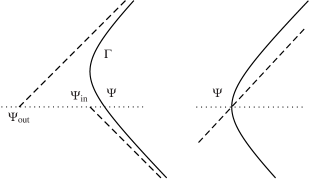
Figure 1: Interacting path $\Gamma$ with asymptotes in $\mathbb{R}\times\mathcal{H}$, free and interacting path through $\Psi$

To abstract from the inessential, one would like to consider the limits $\Psi_{\pm}$ of $U^{\prime}(t)\Psi$ for $t\rightarrow\pm\infty$. But such limits of a unitary, nontrivial one-parameter group do not exist: $U^{\prime}(s+t)=U^{\prime}(s)U^{\prime}(t)$ implies $\Psi_{\pm}=U^{\prime}(s)\Psi_{\pm}$ and $U^{\prime}(t)\Psi-\Psi_{\pm}=U^{\prime}(t)(\Psi-\Psi_{\pm})$. As $U^{\prime}(t)$ is unitary the norm of this difference is time independent and vanishes in the limit only if it vanishes for all times. i.e. only if $\Psi$ does not move [10].

A unitary, nontrivial group of motion has no limit.

The interacting evolution of scattering states $\Psi$ can at best approach the free evolution by $U(t)=\mathrm{e}^{-\mathrm{i}Ht}$ of asymptotic states $\Psi_{\pm}$ such that $U^{\prime}(t)\Psi-U(t)\Psi_{\pm}$ or equivalently $U^{\prime-1}(t)U(t)\Psi_{\pm}$ converge for $t\rightarrow\pm\infty$. There have to exist the strong limits

$$\Omega_{+}=\operatorname*{s-lim\,}_{t\rightarrow\infty}\Omega(t)\ ,\ \Omega_{-}=\operatorname*{s-lim\,}_{t\rightarrow-\infty}\Omega(t)\ ,\ \Omega(t)=\mathrm{e}^{\mathrm{i}H^{\prime}\,t}\,\mathrm{e}^{-\mathrm{i}H\,t}\ ,\$$ (5)

that the interacting path through each scattering state $\Psi$, which is orthogonal to all bound states of $H^{\prime}$, has a past and a future free asymptote through states $\Psi_{\text{in}}$ and $\Psi_{\text{out}}$ with

$$\lim_{t\rightarrow\infty}\Omega(t)\,\Psi_{\text{out}}=\Omega_{+}\Psi_{\text{out}}=\Psi\ ,\ \lim_{t\rightarrow-\infty}\Omega(t)\,\Psi_{\text{in}}=\Omega_{-}\Psi_{\text{in}}=\Psi\ .$$ (6)

The strong limit of $\Omega(t)$ for $t\rightarrow\infty$ demands that for each $\varepsilon>0$ and for each scattering state $\Psi$ there is a time $T$ such that $\lVert(\Omega(t)-\Omega_{+})\Psi\rVert<\varepsilon\lVert\Psi\rVert$ for all $t>T$. This is a weaker condition than the uniform limit that $T$ be independent of $\Psi$.

To ask even stronger for the uniform limit of $\Omega(t)$ would require too much because at each time $T$ there are states which have not reached or left the interaction region.

$\Omega_{+}$ and $\Omega_{-}$ are the generalized wave operators or Møller operators.

In more detail we write $\Omega_{\pm}(H^{\prime},H)$ to display the involved Hamiltonians. One has $\Omega_{\pm}(H^{\prime},H)^{\star}=\Omega_{\pm}(H,H^{\prime})$ and $\Omega_{\pm}(A,B)\,\Omega_{\pm}(B,C)=\Omega_{\pm}(A,C)$ [10].

By construction the wave operators $\Omega_{\pm}$ do not commute with free time translations but intertwine $H^{\prime}$ unitarily with its corresponding $H$,

$$\Omega_{\pm}=\operatorname*{s-lim\,}_{t\rightarrow\pm\infty}\mathrm{e}^{\mathrm{i}\,H^{\prime}\,(t+a)}\mathrm{e}^{-\mathrm{i}\,H\,(t+a)}=\mathrm{e}^{\mathrm{i}\,H^{\prime}a}\Omega_{\pm}\mathrm{e}^{-\mathrm{i}\,H\,a}\ ,\quad\mathrm{e}^{\mathrm{i}\,H^{\prime}\,a}\Omega_{\pm}=\Omega_{\pm}\mathrm{e}^{\mathrm{i}\,H\,a}\ .$$ (7)

Differentiation at $a=0$ shows

$$H^{\prime}\Omega_{\pm}\Psi=\Omega_{\pm}H\Psi\ ,\ H^{\prime}=\Omega_{\pm}H\Omega_{\pm}^{-1}\ ,$$ (8)

for all smooth scattering states $\Psi$. On these states $H^{\prime}$ is unitarily equivalent to $H$.

But $H^{\prime}$ must not commute with $H$, otherwise it commutes with $\Omega(t)$ and equals $H$ if $\Omega_{\pm}$ exists. Thus, implementing translational invariance one must not require $H^{\prime}$ to commute with the unitary representation $U_{a}=\mathrm{e}^{\mathrm{i}Pa}$ of translations.

3 Cross Section and Luminosity

We employ the Schrödinger picture and view time evolutions as worldlines $\set{(t,\Psi(t))}$ in quantum spacetime $\mathbb{R}\times\mathcal{H}$. Interaction makes the worldlines of many-particle states depart from the free time evolution. $\Psi_{\text{in}}$ and $\Psi_{\text{out}}$ are not states with momenta which are all directed towards or away from a scattering region. Rather they are the initial states of the future or past asymptotes which in the long run will automatically develop this property. They only have to be many-particle states in the continuous spectrum of $M^{\prime}$. That a state lies on an interacting trajectory is not a property of the state but a relation of the state and the path. Such a relation does not contradict the additional relation that the same state also lies on a free trajectory. By themselves states have no time evolution and are neither interacting nor free, they are just states and determine the probabilities of the results of all measurements.

Similarly in classical mechanics particles may traverse Kepler ellipses or straight lines, but this does not make the points of these curves elliptic or straight. Nitpicking as the remark may seem, it spares the vain endeavours to construct interacting fields or the futile considerations what an interacting Lorentz boost should be. Such denominations are widespread but misleading: to be interacting is a property not of states but of time evolutions. Scattering theory compares different time evolutions.

By the basic assumption of quantum theory the probability for a result $a_{i}$ (which for simplicity we take to be labeled by some discrete index $i$) to occur if the state $\Psi$ is measured with a perfect apparatus $A$, is given by

$$w(i,A,\Psi)=|\Braket{\Lambda_{i}}{\Psi}|^{2}\ ,$$ (9)

where $\Lambda_{i}$ is the state which yields $a_{i}$ with certainty.

In the Heisenberg picture not the states evolve in the course of time $t$ but the operators which represent the measuring devices and enter (9) by their eigenvectors $\Lambda$,

$$\Braket{\Lambda(0)}{\vphantom{U(t)^{\star}}U(t)\Psi(0)}_{\text{Schr\"{o}dinger}}=\Braket{U(t)^{\star}\Lambda(0)}{\Psi(0)}_{\text{Heisenberg}}\ .$$ (10)

The Heisenberg picture is invertibly related to the Schrödinger picture and in this sense equivalent. But to ascribe the motion of several particles, which move relative to each other and scatter, to the measuring devices is as counterintuitive and misleading as the Ptolemaic system which describes the orbits of the planets in highly unsuitable, though admissible, coordinates in which the earth does not rotate and does not orbit the sun. Try e.g. to understand the simple notion of the spacetime overlap of colliding wave packets (21) in the Heisenberg picture.

The Schrödinger picture does not rule out to consider time independent states, such as $\Psi_{\text{in}}$ or $\Psi_{\text{out}}$, the initial states of the asymptotes of interacting paths, nor does it preclude time dependent operators such as free fields. They are used to construct a local, relativistic $S$-matrix. Time dependent fields do not have to represent measuring devices in the Heisenberg picture, notwithstanding axiomatic systems which call them ‘observables’.

The scattering matrix or $S$-matrix is the map

$$S:\Psi_{\text{in}}\mapsto\Psi_{\text{out}}\ ,\ S=\Omega_{+}^{\star}\Omega_{-}=\operatorname*{s-lim\,}_{t,\,t^{\prime}\rightarrow\infty}\,\mathrm{e}^{\mathrm{i}Ht}\mathrm{e}^{-\mathrm{i}H^{\prime}(t+t^{\prime})}\mathrm{e}^{\mathrm{i}Ht^{\prime}}\ .$$ (11)

Its matrix elements are scalar products of out- and in-states, $\braket{\Phi_{\text{in}}}{\Psi_{\text{out}}}=\braket{\Phi_{\text{in}}}{S\Psi_{\text{in}}}$.

By construction and by (7) the $S$-matrix commutes with temporal translations

$$S=\mathrm{e}^{\mathrm{i}\,H\,a}\,S\,\mathrm{e}^{-\mathrm{i}\,H\,a}\ ,\ [H,S]=0\ .$$ (12)

If the $S$-matrix commutes with Lorentztransformations, $U_{\Lambda}S\,U_{\Lambda}{}^{-1}=S$, then $S$ commutes not only with $H=P^{0}$ but with all momenta $P^{m}$ and with all $U_{a,\Lambda}$. Conservation of $P^{m}$ does not require $H^{\prime}$ to commute with $P^{0}$.

The relativistic $S$-matrix in the momentum basis, not the basis independent $S$-matrix by itself, contains the experimentally available information about the interacting particles. Consider the transfer matrix $T:=\mathrm{i}(S-1)$. Applied to an incoming two-particle state $\Psi$, omitting spin indices, using the short hand $q=(q_{1},\dots q_{n})$ and the scalar product of one-particle states on mass shells $\mathcal{M}_{m}=\set{p:p^{0}=\sqrt{m^{2}+\mathchoice{\mbox{\boldmath$\displaystyle\mathbf{p}$}}{\mbox{\boldmath$\textstyle\mathbf{p}$}}{\mbox{\boldmath$\scriptstyle\mathbf{p}$}}{\mbox{\boldmath$\scriptscriptstyle\mathbf{p}$}}^{2}},\mathchoice{\mbox{\boldmath$\displaystyle\mathbf{p}$}}{\mbox{\boldmath$\textstyle\mathbf{p}$}}{\mbox{\boldmath$\scriptstyle\mathbf{p}$}}{\mbox{\boldmath$\scriptscriptstyle\mathbf{p}$}}\in\mathbb{R}^{3}}\subset\mathbb{R}^{4}$,

$$\braket{\Phi}{\Psi}=\int\!\!\operatorname{\tilde{d}\!}p\,\Phi(p)^{*}\,\Psi(p)\ ,\ \operatorname{\tilde{d}\!}p=\frac{\operatorname{d}^{3}p}{(2\pi)^{3}\,2\sqrt{m^{2}+\mathchoice{\mbox{\boldmath$\displaystyle\mathbf{p}$}}{\mbox{\boldmath$\textstyle\mathbf{p}$}}{\mbox{\boldmath$\scriptstyle\mathbf{p}$}}{\mbox{\boldmath$\scriptscriptstyle\mathbf{p}$}}^{3}}}\ ,$$ (13)

its reduced kernel $\Braket{q}{\mathfrak{T}}{p_{1},p_{2}}$ is defined by

$$\mathrm{i}(S-{\mathbf{1}})\Psi(q)=(2\pi)^{4}\!\!\int\!\tilde{\operatorname{d}}p_{1}\,\tilde{\operatorname{d}}p_{2}\,\delta^{4}(p_{1}+p_{2}-\sum_{i=1}^{n}q_{i})\Braket{q}{\mathfrak{T}}{p_{1},p_{2}}\Psi(p_{1},p_{2})\,.$$ (14)

It determines the partial cross sections for the production of $n$ particles with momenta $q$ in some domain $\Delta_{n}$ (denoting $\operatorname{\tilde{d}\!}q_{1}\dots\operatorname{\tilde{d}\!}q_{n}$ by $\operatorname{\tilde{d}\!}^{\,n}\!q$)

$$\sigma_{(p_{1},p_{2})\rightarrow\Delta_{n}}=\frac{(2\pi)^{4}}{4\sqrt{(p_{1}\cdot p_{2})^{2}-m_{1}^{2}m_{2}^{2}}}\int_{\Delta_{n}}\!\!\tilde{\operatorname{d}}^{n}\!q\,\delta^{4}(p_{1}+p_{2}-\sum_{i=1}^{n}q_{i})\,\bigl{|}\Braket{q}{\mathfrak{T}}{p_{1},p_{2}}\bigr{|}^{2}\ .$$ (15)

We give a simple proof of this well-known basic relation of quantum scattering theory to observable physics, which has the virtue to also determine the luminosity, which is basic to our optical perception of the world.

Recall that the wave function $\Phi=(S-1)\Psi$ is smooth if $\Psi$ is smooth: the relativistic $S$-matrix commutes with Poincaré transformations and maps the domain of the algebra of the generators, rapidly decreasing smooth wave functions [12], to itself. The $\delta^{4}$-function in (14) is not a singularity but reduces the integral on $\mathcal{M}_{1}\times\mathcal{M}_{2}$ to the compact submanifold $p_{1}+p_{2}=\sum_{i=1}^{n}q_{i}$, the phase space of the reaction. Similarly

$$\bigl{(}(S^{\star}-1)\chi\bigr{)}(p_{1},p_{2})=\mathrm{i}(2\pi)^{4}\!\!\int\!\tilde{\operatorname{d}}^{n}q\,\delta^{4}(p_{1}+p_{2}-\sum_{i=1}^{n}q_{i})\,\Braket{q}{\mathfrak{T}}{p_{1},p_{2}}^{*}\chi(q)$$ (16)

is smooth if $\chi$ is smooth.

By the generalization of (9) to results in a continuum, the integral $\int_{\Delta_{n}}\!\operatorname{\tilde{d}\!}^{n}q\,\Phi^{*}(q)\,\Phi(q)$ is the probability to find after the scattering $n$ particles with momenta $q=(q_{1},\dots q_{n})$ in the domain $\Delta_{n}$. Inserting (14) yields 4 momentum integrations with a product of $\delta^{4}$-functions of different variables

$$\delta^{4}(p_{1}+p_{2}-\sum_{i=1}^{n}q_{i})\,\delta^{4}(p^{\prime}_{1}+p^{\prime}_{2}-\sum_{i=1}^{n}q_{i})=\delta^{4}(p_{1}+p_{2}-\sum_{i=1}^{n}q_{i})\,\delta^{4}(p^{\prime}_{1}+p^{\prime}_{2}-p_{1}-p_{2})$$

$$=\delta^{4}(p_{1}+p_{2}-\sum_{i=1}^{n}q_{i})\,\frac{1}{(2\pi)^{4}}\int\!\operatorname{d}^{4}x\ \mathrm{e}^{\mathrm{i}\,(p^{\prime}_{1}+p^{\prime}_{2}-p_{1}-p_{2})\,x}\ .$$ (17)

So the second $\delta^{4}$-function can be exchanged by the spacetime integral over the products at $x$ of plane waves for each of the integration variables $(p_{1},p_{2},p^{\prime}_{1},p^{\prime}_{2})$. More precisely this applies if multiplied with smooth test functions, which is why we remarked that $\Psi$ and $(S-1)\Psi$ are smooth and that the $\delta$-functions only reduce integrations to integrals over submanifolds.

In scattering of distinguishable particles the incoming state is a product of momentum wave packets, $\Psi(p_{1},p_{2})=\Psi_{1}(p_{1})\Psi_{2}(p_{2})$, with support contained in small neighbourhoods around ${\mathrm{bar}p}_{1}$ and ${\mathrm{bar}p}_{2}$. For small enough neighbourhood the smooth $\mathfrak{T}$-function does not vary appreciably. So we extract

$$\begin{gathered}\delta^{4}(p_{1}+p_{2}-\sum_{i=1}^{n}q_{i})\,\Braket{q}{\mathfrak{T}}{p_{1},p_{2}}\Braket{q}{\mathfrak{T}}{p^{\prime}_{1},p^{\prime}_{2}}^{*}/\sqrt{p_{1}^{0}\,p_{1}^{\prime\,0}\,p_{2}^{0}\,p_{2}^{\prime\,0}}\\ \sim\delta^{4}(\mathrm{bar}p_{1}+\mathrm{bar}p_{2}-\sum_{i=1}^{n}q_{i})\,|\!\Braket{q}{\mathfrak{T}}{\mathrm{bar}p_{1},\mathrm{bar}p_{2}}|^{2}/(\mathrm{bar}p_{1}^{0}\mathrm{bar}p_{2}^{0})\end{gathered}$$ (18)

as if constant from the $(p_{1},p_{2},p^{\prime}_{1},p^{\prime}_{2})$-integrations of the wave packets. Each of these $p$-integrations is of the form

$$\tilde{\Psi}(x)=\sqrt{2}\int\!\operatorname{\tilde{d}\!}p\,\sqrt{p^{0}}\,\Psi(p)\,\mathrm{e}^{-\mathrm{i}p\,x}$$ (19)

or its complex conjugate and yields in the Schrödinger picture for massive particles the corresponding freely propagating position wave function at $x\in\mathbb{R}^{1,3}$, the remaining integration variable. Dropping the symbol $\ \mathrm{bar}{}\$ we find the momentum $q$ in the domain $\Delta_{n}$ (which must not overlap with the beam) with probability

$$w_{(p_{1},p_{2})\rightarrow\Delta_{n}}=$$ (20)

$$\frac{(2\pi)^{4}}{4p^{0}_{1}p^{0}_{2}}\,\int_{\Delta_{n}}\!\operatorname{\tilde{d}\!}^{n}q\,\delta^{4}(p_{1}+p_{2}-\sum_{i=1}^{n}q_{i})\ |\Braket{q}{\mathfrak{T}}{p_{1},p_{2}}|^{2}\,\int\!\operatorname{d}^{4}x\,|\tilde{\Psi}_{1}(x)|^{2}\,|\tilde{\Psi}_{2}(x)|^{2}\ .$$

It factorizes into the cross section (15) times the integrated luminosity $L$

$$\begin{gathered}w_{(p_{1},p_{2})\rightarrow\Delta_{n}}=\sigma_{(p_{1},p_{2})\rightarrow\Delta_{n}}\,L\ ,\\ L=\frac{\sqrt{(p_{1}\cdot p_{2})^{2}-m_{1}^{2}m_{2}^{2}}}{p_{1}^{0}p_{2}^{0}}\int\!\!\operatorname{d}\!^{\,4}\!x\,|\tilde{\Psi}_{1}(t,\mathchoice{\mbox{\boldmath$\displaystyle\mathbf{x}$}}{\mbox{\boldmath$\textstyle\mathbf{x}$}}{\mbox{\boldmath$\scriptstyle\mathbf{x}$}}{\mbox{\boldmath$\scriptscriptstyle\mathbf{x}$}})|^{2}\,|\tilde{\Psi}_{2}(t,\mathchoice{\mbox{\boldmath$\displaystyle\mathbf{x}$}}{\mbox{\boldmath$\textstyle\mathbf{x}$}}{\mbox{\boldmath$\scriptstyle\mathbf{x}$}}{\mbox{\boldmath$\scriptscriptstyle\mathbf{x}$}})|^{2}\ .\end{gathered}$$ (21)

Even if photons are massless and do not allow for a generator $\textstyle\mathbf{X}$ of translations of spatial momentum, such that strictly speaking they do not have a well-defined position wave function, we take the integrated luminosity (21) to define macroscopic position measurement: to detect an object you shine light on it and register the reflected light. The other way round: a beam of light becomes visible if traversing mist.

During the overlap of wave packets we neglect their spreading which occurs because they are superposed of momenta near $p_{1}$ and $p_{2}$. Then in fixed target scattering the density $|\tilde{\Psi}_{1}|^{2}(t,\mathchoice{\mbox{\boldmath$\displaystyle\mathbf{x}$}}{\mbox{\boldmath$\textstyle\mathbf{x}$}}{\mbox{\boldmath$\scriptstyle\mathbf{x}$}}{\mbox{\boldmath$\scriptscriptstyle\mathbf{x}$}})=\rho_{1}(\mathchoice{\mbox{\boldmath$\displaystyle\mathbf{x}$}}{\mbox{\boldmath$\textstyle\mathbf{x}$}}{\mbox{\boldmath$\scriptstyle\mathbf{x}$}}{\mbox{\boldmath$\scriptscriptstyle\mathbf{x}$}})$ is time independent and the impinging wave packet is rigidly shifted with velocity $\mathchoice{\mbox{\boldmath$\displaystyle\mathbf{v}$}}{\mbox{\boldmath$\textstyle\mathbf{v}$}}{\mbox{\boldmath$\scriptstyle\mathbf{v}$}}{\mbox{\boldmath$\scriptscriptstyle\mathbf{v}$}}\neq 0$, $|\tilde{\Psi}_{2}|^{2}(t,\mathchoice{\mbox{\boldmath$\displaystyle\mathbf{x}$}}{\mbox{\boldmath$\textstyle\mathbf{x}$}}{\mbox{\boldmath$\scriptstyle\mathbf{x}$}}{\mbox{\boldmath$\scriptscriptstyle\mathbf{x}$}})=\rho_{2}(\mathchoice{\mbox{\boldmath$\displaystyle\mathbf{x}$}}{\mbox{\boldmath$\textstyle\mathbf{x}$}}{\mbox{\boldmath$\scriptstyle\mathbf{x}$}}{\mbox{\boldmath$\scriptscriptstyle\mathbf{x}$}}-\mathchoice{\mbox{\boldmath$\displaystyle\mathbf{v}$}}{\mbox{\boldmath$\textstyle\mathbf{v}$}}{\mbox{\boldmath$\scriptstyle\mathbf{v}$}}{\mbox{\boldmath$\scriptscriptstyle\mathbf{v}$}}t)$. We employ coordinates $\mathchoice{\mbox{\boldmath$\displaystyle\mathbf{x}$}}{\mbox{\boldmath$\textstyle\mathbf{x}$}}{\mbox{\boldmath$\scriptstyle\mathbf{x}$}}{\mbox{\boldmath$\scriptscriptstyle\mathbf{x}$}}=(x,x_{\perp})$ parallel and perpendicular to $\mathchoice{\mbox{\boldmath$\displaystyle\mathbf{v}$}}{\mbox{\boldmath$\textstyle\mathbf{v}$}}{\mbox{\boldmath$\scriptstyle\mathbf{v}$}}{\mbox{\boldmath$\scriptscriptstyle\mathbf{v}$}}=(v,0,0)$ and denote the area densities obtained by integrating the volume densities along the beam by

$$\hat{\rho}(x_{\perp})=\int\!\operatorname{d}\!x\ \rho(x,x_{\perp})\ .$$ (22)

With these specifications the spacetime integral in (21) yields

$$\int\!\!\operatorname{d}\!^{\,2}x_{\perp}\!\int\!\!\operatorname{d}x\ \rho_{1}(x,x_{\perp})\!\int\!\!\operatorname{d}t\,\rho_{2}(x-vt,x_{\perp})=\int\!\!\operatorname{d}\!^{\,2}x_{\perp}\,\hat{\rho}_{1}(x_{\perp})\,\hat{\rho}_{2}(x_{\perp})\,\frac{1}{v}\ .$$ (23)

The beam overlaps the target, $\operatorname{supp}\hat{\rho}_{1}\subset\operatorname{supp}\hat{\rho}_{2}$, else $\Psi_{1}$ is not a target in the beam. Moreover, within $\operatorname{supp}\rho_{1}$ the density of the beam $\hat{\rho}_{2}(x_{\perp})=\mathrm{bar}\rho_{2}$ has its average value, at least after taking the mean of measurements with the target randomly positioned in the beam. The remaining integral $\int\!\operatorname{d}\!^{\,2}x_{\perp}\,\hat{\rho}_{1}(x_{\perp})=1$ is the number of targets. With $p_{1}=(m_{1},0,0,0)$, $(p_{1}\cdot p_{2})^{2}-m_{1}^{2}m_{2}^{2}=m_{1}^{2}\mathchoice{\mbox{\boldmath$\displaystyle\mathbf{p}$}}{\mbox{\boldmath$\textstyle\mathbf{p}$}}{\mbox{\boldmath$\scriptstyle\mathbf{p}$}}{\mbox{\boldmath$\scriptscriptstyle\mathbf{p}$}}_{2}^{2}$ and $v=|\mathchoice{\mbox{\boldmath$\displaystyle\mathbf{p}$}}{\mbox{\boldmath$\textstyle\mathbf{p}$}}{\mbox{\boldmath$\scriptstyle\mathbf{p}$}}{\mbox{\boldmath$\scriptscriptstyle\mathbf{p}$}}_{2}|/p_{2}^{0}$ the integrated luminosity for fixed target scattering turns out to be the mean area density of the beam, the inverse of the size $A$ of its transversal section,

$$L_{\text{fixed target}}=\mathrm{bar}\rho_{2}=1/A\ .$$ (24)

The particle is scattered with the same probability $w=\sigma/A$ with which a randomly positioned point in the beam hits a fixed area of size $\sigma$ in the beam. This confirms that $\sigma_{(p_{1},p_{2})\rightarrow\Delta_{n}}$ (15) is the partial cross section of the target.

4 Center Variables

The total momentum $P^{m}$ of an $n$-particle state $\Psi(p_{1},\dots p_{n})$ defines its invariant mass $M$,

$$P^{m}\,\Psi(p_{1},\dots p_{n})=(\sum_{i=1}^{n}p^{m}_{i})\Psi(p_{1},\dots p_{n})\ ,\ M^{2}=P^{2}\ ,$$ (25)

which has a purely continuous spectrum with positive energies and allows to factorize $P^{m}$ as four-velocity $U^{m}$ times $M$

$$P^{m}=U^{m}\,M\ ,\ U^{2}=1\ ,\ [U^{m},M]=0\ .$$ (26)

To separate the motion of the center from the relative motion of the scattering particles, we change the variables of the wave function $\Psi$ from the momenta $(p_{1},\dots p_{n})$, $n\geq 2$, to the constrained center variables $(u,q)$ where

$$u^{m}=\frac{\sum_{i}p^{m}_{i}}{\sqrt{(\sum_{j}p_{j})^{2}}}\ ,\ u^{2}=1\ ,$$ (27)

is the four-velocity of the center. It is well-defined unless all momenta are lightlike and colinear, a Lorentz invariant submanifold $S^{2}\times\mathbb{R}^{n}$ which is outside the domain of scattering theory. To obtain $q=(q_{1},\dots q_{n})\in\mathbb{R}^{3n}$, the relative momenta at rest, we decompose each momentum $p_{i}$ into parts which are parallel and orthogonal to $u$,

$$p_{i}=p_{i\,\parallel}+p_{i\,\perp}\ ,\ p_{i\,\parallel}=(p_{i}\cdot u)\,u\ ,\ p_{i\,\perp}=p_{i}-p_{i\,\parallel}\ ,$$ (28)

and boost each $p_{i\,\perp}$ by the inverse of the Lorentz boost

$$L_{u}=\begin{pmatrix}\sqrt{1+\mathchoice{\mbox{\boldmath$\displaystyle\mathbf{u}$}}{\mbox{\boldmath$\textstyle\mathbf{u}$}}{\mbox{\boldmath$\scriptstyle\mathbf{u}$}}{\mbox{\boldmath$\scriptscriptstyle\mathbf{u}$}}^{2}}&\mathchoice{\mbox{\boldmath$\displaystyle\mathbf{u}$}}{\mbox{\boldmath$\textstyle\mathbf{u}$}}{\mbox{\boldmath$\scriptstyle\mathbf{u}$}}{\mbox{\boldmath$\scriptscriptstyle\mathbf{u}$}}^{\operatorname{T}}\\ \mathchoice{\mbox{\boldmath$\displaystyle\mathbf{u}$}}{\mbox{\boldmath$\textstyle\mathbf{u}$}}{\mbox{\boldmath$\scriptstyle\mathbf{u}$}}{\mbox{\boldmath$\scriptscriptstyle\mathbf{u}$}}&\quad{\mathbf{1}}+\frac{\mathchoice{\mbox{\boldmath$\displaystyle\mathbf{u}$}}{\mbox{\boldmath$\textstyle\mathbf{u}$}}{\mbox{\boldmath$\scriptstyle\mathbf{u}$}}{\mbox{\boldmath$\scriptscriptstyle\mathbf{u}$}}\,\mathchoice{\mbox{\boldmath$\displaystyle\mathbf{u}$}}{\mbox{\boldmath$\textstyle\mathbf{u}$}}{\mbox{\boldmath$\scriptstyle\mathbf{u}$}}{\mbox{\boldmath$\scriptscriptstyle\mathbf{u}$}}^{\operatorname{T}}}{1+\sqrt{1+\mathchoice{\mbox{\boldmath$\displaystyle\mathbf{u}$}}{\mbox{\boldmath$\textstyle\mathbf{u}$}}{\mbox{\boldmath$\scriptstyle\mathbf{u}$}}{\mbox{\boldmath$\scriptscriptstyle\mathbf{u}$}}^{2}}}\ ,\end{pmatrix}$$ (29)

which maps $\underline{u}=(1,0,0,0)$ to the four-velocity $u=(\sqrt{1+\mathchoice{\mbox{\boldmath$\displaystyle\mathbf{u}$}}{\mbox{\boldmath$\textstyle\mathbf{u}$}}{\mbox{\boldmath$\scriptstyle\mathbf{u}$}}{\mbox{\boldmath$\scriptscriptstyle\mathbf{u}$}}^{2},}\mathchoice{\mbox{\boldmath$\displaystyle\mathbf{u}$}}{\mbox{\boldmath$\textstyle\mathbf{u}$}}{\mbox{\boldmath$\scriptstyle\mathbf{u}$}}{\mbox{\boldmath$\scriptscriptstyle\mathbf{u}$}})$, to

$$q_{i}=(L_{u})^{-1}p_{i\,\perp}\ .$$ (30)

Its $0$-component vanishes, $0=u\cdot p_{i\,\perp}=(L_{u}^{-1}u)\cdot(L_{u}^{-1}p_{i\,\perp})=\underline{u}\cdot q_{i}=q_{i}^{0}$: each $q_{i}=(0,\mathchoice{\mbox{\boldmath$\displaystyle\mathbf{q}$}}{\mbox{\boldmath$\textstyle\mathbf{q}$}}{\mbox{\boldmath$\scriptstyle\mathbf{q}$}}{\mbox{\boldmath$\scriptscriptstyle\mathbf{q}$}}_{i})$ lies in $\mathbb{R}^{3}$. By definition, $\sum_{i}p_{i}=\sum_{i}p_{i\parallel}$, so the $q_{i}$ are constrained,

$$0=\sum_{i=1}^{n}q_{i}\ .$$ (31)

Because of $m_{i}{}^{2}=(p_{i\,\parallel}+p_{i\,\perp})^{2}=(p_{i}\cdot u)^{2}+q_{i}^{2}$, one has $(p_{i}\cdot u)^{2}=m_{i}^{2}+\mathchoice{\mbox{\boldmath$\displaystyle\mathbf{q}$}}{\mbox{\boldmath$\textstyle\mathbf{q}$}}{\mbox{\boldmath$\scriptstyle\mathbf{q}$}}{\mbox{\boldmath$\scriptscriptstyle\mathbf{q}$}}_{i}^{2}$ and the momenta $p_{i}$ in terms of the constrained center variables are

$$p_{i}(u,q)=\sqrt{m_{i}^{2}+\mathchoice{\mbox{\boldmath$\displaystyle\mathbf{q}$}}{\mbox{\boldmath$\textstyle\mathbf{q}$}}{\mbox{\boldmath$\scriptstyle\mathbf{q}$}}{\mbox{\boldmath$\scriptscriptstyle\mathbf{q}$}}_{i}^{2}}\,u+L_{u}\,q_{i}=\sqrt{m_{i}^{2}+\mathchoice{\mbox{\boldmath$\displaystyle\mathbf{q}$}}{\mbox{\boldmath$\textstyle\mathbf{q}$}}{\mbox{\boldmath$\scriptstyle\mathbf{q}$}}{\mbox{\boldmath$\scriptscriptstyle\mathbf{q}$}}_{i}^{2}}\begin{pmatrix}\sqrt{1+\mathchoice{\mbox{\boldmath$\displaystyle\mathbf{u}$}}{\mbox{\boldmath$\textstyle\mathbf{u}$}}{\mbox{\boldmath$\scriptstyle\mathbf{u}$}}{\mbox{\boldmath$\scriptscriptstyle\mathbf{u}$}}^{2}}\\ \mathchoice{\mbox{\boldmath$\displaystyle\mathbf{u}$}}{\mbox{\boldmath$\textstyle\mathbf{u}$}}{\mbox{\boldmath$\scriptstyle\mathbf{u}$}}{\mbox{\boldmath$\scriptscriptstyle\mathbf{u}$}}\end{pmatrix}+\begin{pmatrix}\mathchoice{\mbox{\boldmath$\displaystyle\mathbf{u}$}}{\mbox{\boldmath$\textstyle\mathbf{u}$}}{\mbox{\boldmath$\scriptstyle\mathbf{u}$}}{\mbox{\boldmath$\scriptscriptstyle\mathbf{u}$}}\cdot\mathchoice{\mbox{\boldmath$\displaystyle\mathbf{q}$}}{\mbox{\boldmath$\textstyle\mathbf{q}$}}{\mbox{\boldmath$\scriptstyle\mathbf{q}$}}{\mbox{\boldmath$\scriptscriptstyle\mathbf{q}$}}_{i}\\ \mathchoice{\mbox{\boldmath$\displaystyle\mathbf{q}$}}{\mbox{\boldmath$\textstyle\mathbf{q}$}}{\mbox{\boldmath$\scriptstyle\mathbf{q}$}}{\mbox{\boldmath$\scriptscriptstyle\mathbf{q}$}}_{i}+\frac{(\mathchoice{\mbox{\boldmath$\displaystyle\mathbf{u}$}}{\mbox{\boldmath$\textstyle\mathbf{u}$}}{\mbox{\boldmath$\scriptstyle\mathbf{u}$}}{\mbox{\boldmath$\scriptscriptstyle\mathbf{u}$}}\cdot\mathchoice{\mbox{\boldmath$\displaystyle\mathbf{q}$}}{\mbox{\boldmath$\textstyle\mathbf{q}$}}{\mbox{\boldmath$\scriptstyle\mathbf{q}$}}{\mbox{\boldmath$\scriptscriptstyle\mathbf{q}$}}_{i})\,\mathchoice{\mbox{\boldmath$\displaystyle\mathbf{u}$}}{\mbox{\boldmath$\textstyle\mathbf{u}$}}{\mbox{\boldmath$\scriptstyle\mathbf{u}$}}{\mbox{\boldmath$\scriptscriptstyle\mathbf{u}$}}}{1+\sqrt{1+\mathchoice{\mbox{\boldmath$\displaystyle\mathbf{u}$}}{\mbox{\boldmath$\textstyle\mathbf{u}$}}{\mbox{\boldmath$\scriptstyle\mathbf{u}$}}{\mbox{\boldmath$\scriptscriptstyle\mathbf{u}$}}^{2}}}\end{pmatrix}\ .$$ (32)

By $\sum_{i}p_{i}=\sum_{i}(p_{i}\cdot u)\,u=M\,u$ the invariant mass $M$ is the energy in the rest system

$$(M\Psi)(u,q)=M(q)\,\Psi(u,q)\ ,\ M(q)=\sum_{i=1}^{n}\sqrt{m_{i}^{2}+\mathchoice{\mbox{\boldmath$\displaystyle\mathbf{q}$}}{\mbox{\boldmath$\textstyle\mathbf{q}$}}{\mbox{\boldmath$\scriptstyle\mathbf{q}$}}{\mbox{\boldmath$\scriptscriptstyle\mathbf{q}$}}_{i}^{2}}\geq\sum_{i}m_{i}\ .$$ (33)

The momenta $p_{i}$ and $u$ Lorentz transform as four-vectors, $u\mapsto\Lambda u$, while for given $u$ the relative momenta $q_{i}$ are Wigner rotated by $W(\Lambda,u)=L_{\Lambda u}^{-1}\Lambda L_{u}\in$SO$(3)$.

The constraint $\sum_{i}q_{i}=0$ complicates $M(q)$. Solving it by $q_{n}=-\sum_{i=1}^{n-1}q_{i}$, the mass $M(q)=\sum^{\prime}\sqrt{m_{i}^{2}+\mathchoice{\mbox{\boldmath$\displaystyle\mathbf{q}$}}{\mbox{\boldmath$\textstyle\mathbf{q}$}}{\mbox{\boldmath$\scriptstyle\mathbf{q}$}}{\mbox{\boldmath$\scriptscriptstyle\mathbf{q}$}}_{i}^{2}}+\sqrt{m_{n}^{2}+(\sum^{\prime}\mathchoice{\mbox{\boldmath$\displaystyle\mathbf{q}$}}{\mbox{\boldmath$\textstyle\mathbf{q}$}}{\mbox{\boldmath$\scriptstyle\mathbf{q}$}}{\mbox{\boldmath$\scriptscriptstyle\mathbf{q}$}}_{i})^{2}}$ depends for $n\geq 3$ not only on $\mathchoice{\mbox{\boldmath$\displaystyle\mathbf{q}$}}{\mbox{\boldmath$\textstyle\mathbf{q}$}}{\mbox{\boldmath$\scriptstyle\mathbf{q}$}}{\mbox{\boldmath$\scriptscriptstyle\mathbf{q}$}}_{i}^{2}$ but also on so called Hughes-Eckart terms $\mathchoice{\mbox{\boldmath$\displaystyle\mathbf{q}$}}{\mbox{\boldmath$\textstyle\mathbf{q}$}}{\mbox{\boldmath$\scriptstyle\mathbf{q}$}}{\mbox{\boldmath$\scriptscriptstyle\mathbf{q}$}}_{i}\cdot\mathchoice{\mbox{\boldmath$\displaystyle\mathbf{q}$}}{\mbox{\boldmath$\textstyle\mathbf{q}$}}{\mbox{\boldmath$\scriptstyle\mathbf{q}$}}{\mbox{\boldmath$\scriptscriptstyle\mathbf{q}$}}_{j}$.

Wavefunctions of the relative momenta $(q_{1},\dots q_{n-1})$ together with the spins of the $n$ particles constitute a representation space of rotations SO$(3)$ or SU$(2)$. It decomposes into a sum $\sum_{s}\mathbb{C}^{2s+1}\otimes\mathcal{I}_{s}$ of multiplets on which the representation acts by multiplication with unitary spin-$s$ matrices with skew hermitian generators $\Gamma_{ij}$ leaving pointwise invariant the Hilbert space $\mathcal{I}_{s}$ of functions $f(r)$ of $d_{n}$ rotation invariant variables $r$ ($d_{2}=1$, $d_{n}=3(n-2)$ for $n>2$). Each of these spin-$s$ multiplets of SO$(3)$ induces a representation $U_{a,\Lambda}$ of the Poincaré group $\mathfrak{P}$ in the space $\mathcal{H}_{s}\otimes\mathcal{I}_{s}$ of wave functions $\Psi(u,r)$ of the center’s four-velocity $u$, $u^{2}=1$, and of the invariants $r$. The generators of $U_{a,\mathrm{e}^{\omega}}=\mathrm{e}^{\mathrm{i}aP}\mathrm{e}^{-\mathrm{i}\omega^{mn}M_{mn}/2}$, $M_{mn}=-M_{nm}$, act on these states by [2]

$$P^{m}=U^{m}\,M\ ,\ \bigl{(}U^{m}\Psi\bigr{)}(u,r)=u^{m}\,\Psi(u,r)\ ,\ \bigl{(}M\Psi\bigr{)}(u,r)=M(r)\,\Psi(u,r)\ ,$$ (34)

$$\begin{aligned} \bigl{(}-\mathrm{i}M_{ij}\Psi\bigr{)}(u,r)&=-\bigl{(}u^{i}\partial_{u^{j}}-u^{j}\partial_{u^{i}}\bigr{)}\Psi(u,r)+\Gamma_{ij}\Psi(u,r)\ ,\\ \bigl{(}-\mathrm{i}M_{0i}\Psi\bigr{)}(u,r)&=\sqrt{1+\mathchoice{\mbox{\boldmath$\displaystyle\mathbf{u}$}}{\mbox{\boldmath$\textstyle\mathbf{u}$}}{\mbox{\boldmath$\scriptstyle\mathbf{u}$}}{\mbox{\boldmath$\scriptscriptstyle\mathbf{u}$}}^{2}}\,\partial_{u^{i}}\Psi(u,r)+\Gamma_{ij}\frac{u^{j}}{1+\sqrt{1+\mathchoice{\mbox{\boldmath$\displaystyle\mathbf{u}$}}{\mbox{\boldmath$\textstyle\mathbf{u}$}}{\mbox{\boldmath$\scriptstyle\mathbf{u}$}}{\mbox{\boldmath$\scriptscriptstyle\mathbf{u}$}}^{2}}}\Psi(u,r)\ .\end{aligned}$$ (35)

The states $\Psi$ are smooth not only as a function of $u$ but within open neighbourhoods also of the variables $r$, if they are smooth functions of $(p_{1}\dots p_{n})$ on each mass shell as is required for $\Psi$ to be in the domain of the generators which act by the product rule.

For a two-particle system and an observer at rest the Hamiltonian $P^{0}=U^{0}\,M$ is

$$H=\sqrt{1+\mathchoice{\mbox{\boldmath$\displaystyle\mathbf{u}$}}{\mbox{\boldmath$\textstyle\mathbf{u}$}}{\mbox{\boldmath$\scriptstyle\mathbf{u}$}}{\mbox{\boldmath$\scriptscriptstyle\mathbf{u}$}}^{2}}\bigl{(}\sqrt{m_{1}^{2}+\mathchoice{\mbox{\boldmath$\displaystyle\mathbf{q}$}}{\mbox{\boldmath$\textstyle\mathbf{q}$}}{\mbox{\boldmath$\scriptstyle\mathbf{q}$}}{\mbox{\boldmath$\scriptscriptstyle\mathbf{q}$}}^{2}}+\sqrt{m_{2}^{2}+\mathchoice{\mbox{\boldmath$\displaystyle\mathbf{q}$}}{\mbox{\boldmath$\textstyle\mathbf{q}$}}{\mbox{\boldmath$\scriptstyle\mathbf{q}$}}{\mbox{\boldmath$\scriptscriptstyle\mathbf{q}$}}^{2}}\bigr{)}=\sqrt{1+\mathchoice{\mbox{\boldmath$\displaystyle\mathbf{u}$}}{\mbox{\boldmath$\textstyle\mathbf{u}$}}{\mbox{\boldmath$\scriptstyle\mathbf{u}$}}{\mbox{\boldmath$\scriptscriptstyle\mathbf{u}$}}^{2}}\bigl{(}m_{1}+m_{2}+\frac{\mathchoice{\mbox{\boldmath$\displaystyle\mathbf{z}$}}{\mbox{\boldmath$\textstyle\mathbf{z}$}}{\mbox{\boldmath$\scriptstyle\mathbf{z}$}}{\mbox{\boldmath$\scriptscriptstyle\mathbf{z}$}}^{2}}{2\mu}\bigr{)}$$ (36)

where $1/\mu=1/m_{1}+1/m_{2}$. The function $\mathchoice{\mbox{\boldmath$\displaystyle\mathbf{q}$}}{\mbox{\boldmath$\textstyle\mathbf{q}$}}{\mbox{\boldmath$\scriptstyle\mathbf{q}$}}{\mbox{\boldmath$\scriptscriptstyle\mathbf{q}$}}^{2}(\mathchoice{\mbox{\boldmath$\displaystyle\mathbf{z}$}}{\mbox{\boldmath$\textstyle\mathbf{z}$}}{\mbox{\boldmath$\scriptstyle\mathbf{z}$}}{\mbox{\boldmath$\scriptscriptstyle\mathbf{z}$}}^{2})$ exists by the implicit function theorem. Explicitly it is given by

$$\mathchoice{\mbox{\boldmath$\displaystyle\mathbf{q}$}}{\mbox{\boldmath$\textstyle\mathbf{q}$}}{\mbox{\boldmath$\scriptstyle\mathbf{q}$}}{\mbox{\boldmath$\scriptscriptstyle\mathbf{q}$}}^{\,2}=\frac{1}{4}(m^{2}-2(m_{1}^{2}+m_{2}^{2})+(m_{1}^{2}-m_{2}^{2})^{2}/m^{2})\ ,\ m^{2}(\mathchoice{\mbox{\boldmath$\displaystyle\mathbf{z}$}}{\mbox{\boldmath$\textstyle\mathbf{z}$}}{\mbox{\boldmath$\scriptstyle\mathbf{z}$}}{\mbox{\boldmath$\scriptscriptstyle\mathbf{z}$}}^{2})=\bigl{(}m_{1}+m_{2}+\mathchoice{\mbox{\boldmath$\displaystyle\mathbf{z}$}}{\mbox{\boldmath$\textstyle\mathbf{z}$}}{\mbox{\boldmath$\scriptstyle\mathbf{z}$}}{\mbox{\boldmath$\scriptscriptstyle\mathbf{z}$}}^{2}/(2\mu)\bigr{)}^{2}\ .$$ (37)

To quadratic order in the velocities, $H$ is the nonrelativistic energy of the center of mass and of the relative motion confirming that the center variables generalize the center of mass coordinates to relativistic motion. However, the free relativistic Hamiltonian is not the sum of the Hamiltonians of the center and the relative motion but their product.

Let the states $\Psi$, which the standard observer $\mathcal{O}$ measures with devices $A$, be related by the unitary representation $V_{a,\Lambda}$ of $\mathfrak{P}$ to the states $\Psi_{a,\Lambda}$, which Poincaré transformed observers $\mathcal{O}_{a,\Lambda}$ measure with the same results with their devices $A_{a,\Lambda}$,

$$A_{a,\Lambda}=V_{a,\Lambda}\,A\,V_{a,\Lambda}{}^{-1}\ ,\ \Psi_{a,\Lambda}=V_{a,\Lambda}\Psi\ ,\ w(i,A,\Psi)=w(i,A_{a,\Lambda},\Psi_{a,\Lambda})\ .$$ (38)

To satisfy the Poincaré algebra, the generators $\hat{P}^{m}=U^{m}\,\hat{M}$ of translations $V_{a,{\mathbf{1}}}$ simply have to employ some hermitian, positive $\hat{M}$ which commutes with the four-velocity $U^{m}$ and with the Lorentz generators $M_{mn}$. However, only if $\hat{M}$ is a multiple of $1$, do the observers agree on all Poincaré invariant measurements with devices $1\otimes\hat{A}$, which only act on the invariant arguments $r$,

$$V_{a,\mathrm{e}^{\omega}}=\mathrm{e}^{\mathrm{i}\,U\cdot a}\mathrm{e}^{-\mathrm{i}\,\omega^{mn}M_{mn}/2}\ .$$ (39)

This is the unique (up to the scale of $a$), maximal degenerate representation of $\mathfrak{P}$ on many particle states. These transformations $V_{a,\Lambda}$ correspond one-to-one to the observers $\mathcal{O}_{a,\Lambda}$. As their translation is generated by the four-velocity $U$, a superposition of nearly mass degenerate particles is seen by translated observers as the same superposition multiplied with a common, mass independent phase rather than an oscillated superposition with changed relative phases.

For the interaction $H^{\prime}$ to be Poincaré covariant it has to commute with the translations $V_{a,{\mathbf{1}}}$ of observers. Hence it commutes with $U^{m}$. And it has to Lorentz transform as $0$-component $H^{\prime}=P^{\prime\,0}$ of a four-vector,

$$[U^{m},H^{\prime}]=0\ ,\ V_{a,\Lambda}\,P^{\prime\,0}\,V_{a,\Lambda}{}^{-1}=\bigl{(}\Lambda^{-1}\bigr{)}{}^{0}{}_{m}P^{\prime m}\ .$$ (40)

But if $H^{\prime}$ commutes with the hermitian, positive operator $U^{0}=\sqrt{1+\mathchoice{\mbox{\boldmath$\displaystyle\mathbf{U}$}}{\mbox{\boldmath$\textstyle\mathbf{U}$}}{\mbox{\boldmath$\scriptstyle\mathbf{U}$}}{\mbox{\boldmath$\scriptscriptstyle\mathbf{U}$}}^{2}}$ then both have a common spectral resolution and $M^{\prime}=H^{\prime}/U^{0}$ is a well-defined hermitian and Lorentz invariant operator,

$$H^{\prime}=U^{0}\,M^{\prime}\ ,\ P^{\prime\,m}=U^{m}\,M^{\prime}\ ,\ [M^{\prime},U^{m}]=0\ ,\ [M^{\prime},M_{mn}]=0\ .$$ (41)

Hence the Møller operators are Lorentz invariant,

$$\begin{gathered}\lim_{t\rightarrow\pm\infty}\bigl{(}\mathrm{e}^{\mathrm{i}\,u^{0}\,M^{\prime}\,t}\mathrm{e}^{-\mathrm{i}\,u^{0}\,M\,t}\Psi\bigr{)}(u,r)=\lim_{t^{\prime}\rightarrow\pm\infty}\bigl{(}\mathrm{e}^{\mathrm{i}\,M^{\prime}\,t^{\prime}}\mathrm{e}^{-\mathrm{i}\,M\,t^{\prime}}\Psi\bigr{)}(u,r)\ ,\\ \Omega_{\pm}(H^{\prime},H)=\Omega_{\pm}(M^{\prime},M)\ .\end{gathered}$$ (42)

So the $S$-matrix commutes with Lorentz transformations. By construction it commutes with $H=P^{0}$ (12), hence it commutes with all $U_{a,\Lambda}$ and not only with $V_{a,\Lambda}$,

$$U_{a,\Lambda}\,S=S\,U_{a,\Lambda}\ .$$ (43)

To commute with $U^{m}$ is a weaker restriction of $H^{\prime}$ than to commute with $P^{m}$. The latter restriction excludes scattering, as $\Omega(t)=\mathrm{e}^{\mathrm{i}(H-H^{\prime})t}$ has a limit only if $H=H^{\prime}$.

Therefore, in a basis of $\mathcal{I}_{s}$ in which $M$ acts multiplicatively, $(Mf)(r)=m(r)f(r)$, the interacting mass $M^{\prime}$ must not be multiplicative. For example $M^{\prime}=M+V$ can be a sum with a potential $V(\mathchoice{\mbox{\boldmath$\displaystyle\mathbf{x}$}}{\mbox{\boldmath$\textstyle\mathbf{x}$}}{\mbox{\boldmath$\scriptstyle\mathbf{x}$}}{\mbox{\boldmath$\scriptscriptstyle\mathbf{x}$}})$ where the position operator $\textstyle\mathbf{x}$ constitutes Heisenberg pairs $[x^{i},z^{j}]=\mathrm{i}\delta^{ij}$ with the relative momentum $\textstyle\mathbf{z}$ defined in (36). If $V$ is spherically symmetric then the $S$-matrix commutes not only with rotations but also with boosts as they act for each $u$ by Wigner rotations of $\textstyle\mathbf{z}$ and $\textstyle\mathbf{x}$.

In nonrelativistic theory [10] spherically symmetric potentials with a nontrivial $S$-matrix are known. So also nontrivial relativistic scattering exists mathematically and not only as perturbation series with unknown convergence properties. The relation of $M^{\prime}$ and the time ordered interaction Lagrangian (2) remains to be analyzed.

In the Hamiltonian description of classical relativistic systems one can choose the generators of spatial translations and of rotations to coincide in the free and in the interacting case [9]

$$P^{\prime\,i}\stackrel{{\scriptstyle?}}{{=}}P^{i}\ ,\ M^{\prime}_{ij}=M_{ij}\ ,\ i,j\in\set{1,2,3}\ .$$ (44)

In a quantum system these relations are suggested if one employs ‘pictures’ for the interacting and free time evolution which coincide at some time. As rotations and spatial translations are time independent and coincide at some time, their generators should agree at all times in the different pictures. But these relations exclude interaction: Poincaré covariance requires the interacting Hamiltonian $H^{\prime}$ to commute with the four-velocity $U^{m}$ (40), hence $P^{\prime\,m}=M^{\prime}\,U^{m}$ and $P^{m}=M\,U^{m}$. But then (44) implies $M^{\prime}=M$ and $P^{\prime\,m}=P^{m}$ and excludes scattering.

Moreover, the condition (44) is measurably wrong as shown by the atomic weights of isotopes. Their rate of spatial momentum transferred by their support to prevent free fall, their weight, depends on the binding.

Using (44) and exploiting ingeniously the analyticity of Lorentz transformations, Rudolf Haag proved [3] the absence of interaction and $S=1$ in axiomatic quantum field theory: the Wightman distributions, the vacuum expectation values of local fields, coincide at all times with the ones of free fields if the free and interacting fields coincide at an initial time.

Omitting all conditions the theorem is abbreviated to the statement that the interaction picture only exists if there is no interaction. But it only excludes all theories based on the Wightman axioms. They allow to reconstruct the fields and their transformations from the Wightman distributions up to unitary equivalence [14]. But then, in case that there are no bound states, the distributions cannot distinguish the free from the interacting evolution as both differ only by unitary transformations $\Omega_{\pm}$ (8).

Haag’s theorem is a no-go result of scattering theory as are the facts that a unitary group of motion has no limit, that $\Omega_{\pm}$ require the strong limit not the norm limit and that on scattering states $H$ and $H^{\prime}$ are unitarily equivalent but must not commute.

Haag’s theorem is ignored by physicists who calculate successfully scattering amplitudes with Feynman graphs and Poincaré invariant rules to extract finite parts of products of free fields. These calculations need no interacting fields. Strictly speaking $S=\operatorname{T}\exp\,\mathrm{i}\int\operatorname{d}^{4}\!x\,\mathcal{L}_{\text{int}}(x)$ is not a series in an algebra of operator valued distributions as insinuated by the Wightman axioms. Rather, the matrix elements of $S$ are recursively defined finite parts of integrals of products of distributions.

In Feynman graphs the term ‘interacting field’  denotes an argument of the time order $\operatorname{T}$. But time order does not act on operators but on a graded commutative algebra and yields operator valued distributions. The field’s equation of motion [6] in the abbreviated notation $\braket{\,X}:=\braket{\Omega}{X\Omega}$

$$\braket{\,\operatorname{T}\,\mathrm{e}^{\mathrm{i}\int\!\!\mathcal{L}_{\text{int}}}\,\frac{\hat{\partial}\mathcal{L}}{\hat{\partial}\phi}(x)\,\phi(x_{1})\dots\phi(x_{n})}=\braket{\,\operatorname{T}\,\mathrm{e}^{\mathrm{i}\int\!\!\mathcal{L}_{\text{int}}}\,\mathrm{i}\frac{\delta}{\delta\phi(x)}\,\bigl{(}\phi(x_{1})\dots\phi(x_{n})\bigr{)}}$$ (45)

contains the derivative ${\delta}/{\delta\phi(x)}$ confirming: an interacting field in a Feynman graph is an operation in a graded commutative algebra, not an operator in Hilbert space.

5 Position Measurement with Light

Massless particles do not allow a position operator $\textstyle\mathbf{X}$, which generates translations of spatial momentum,

$$\bigl{(}\mathrm{e}^{\mathrm{i}\mathchoice{\mbox{\boldmath$\displaystyle\mathbf{b}$}}{\mbox{\boldmath$\textstyle\mathbf{b}$}}{\mbox{\boldmath$\scriptstyle\mathbf{b}$}}{\mbox{\boldmath$\scriptscriptstyle\mathbf{b}$}}\cdot\mathchoice{\mbox{\boldmath$\displaystyle\mathbf{X}$}}{\mbox{\boldmath$\textstyle\mathbf{X}$}}{\mbox{\boldmath$\scriptstyle\mathbf{X}$}}{\mbox{\boldmath$\scriptscriptstyle\mathbf{X}$}}}\Psi\bigr{)}(\mathchoice{\mbox{\boldmath$\displaystyle\mathbf{p}$}}{\mbox{\boldmath$\textstyle\mathbf{p}$}}{\mbox{\boldmath$\scriptstyle\mathbf{p}$}}{\mbox{\boldmath$\scriptscriptstyle\mathbf{p}$}})=\Psi(\mathchoice{\mbox{\boldmath$\displaystyle\mathbf{p}$}}{\mbox{\boldmath$\textstyle\mathbf{p}$}}{\mbox{\boldmath$\scriptstyle\mathbf{p}$}}{\mbox{\boldmath$\scriptscriptstyle\mathbf{p}$}}-\mathchoice{\mbox{\boldmath$\displaystyle\mathbf{b}$}}{\mbox{\boldmath$\textstyle\mathbf{b}$}}{\mbox{\boldmath$\scriptstyle\mathbf{b}$}}{\mbox{\boldmath$\scriptscriptstyle\mathbf{b}$}})\ .$$ (46)

It enlarges the algebra of the Poincaré generators by Heisenberg partners $X^{j}$ of the spatial momenta,

$$\ [P^{i},P^{j}]=0=[X^{i},X^{j}]\ ,\ [P^{i},X^{j}]=-\mathrm{i}\,\delta^{ij}\ ,\ i,j\in\set{1,\dots D-1}\ .$$ (47)

Together with $P^{0}=\sqrt{\mathchoice{\mbox{\boldmath$\displaystyle\mathbf{P}$}}{\mbox{\boldmath$\textstyle\mathbf{P}$}}{\mbox{\boldmath$\scriptstyle\mathbf{P}$}}{\mbox{\boldmath$\scriptscriptstyle\mathbf{P}$}}^{2}}$ this algebra contains for $D>2$

$$\sum_{j=1}^{D-1}[X^{j},[X^{j},P^{0}]]=-\frac{D-2}{|\mathchoice{\mbox{\boldmath$\displaystyle\mathbf{P}$}}{\mbox{\boldmath$\textstyle\mathbf{P}$}}{\mbox{\boldmath$\scriptstyle\mathbf{P}$}}{\mbox{\boldmath$\scriptscriptstyle\mathbf{P}$}}|}$$ (48)

all powers of $1/|\mathchoice{\mbox{\boldmath$\displaystyle\mathbf{P}$}}{\mbox{\boldmath$\textstyle\mathbf{P}$}}{\mbox{\boldmath$\scriptstyle\mathbf{P}$}}{\mbox{\boldmath$\scriptscriptstyle\mathbf{P}$}}|$. To be in the domain of this algebra, the wave functions have to decrease near $\mathchoice{\mbox{\boldmath$\displaystyle\mathbf{p}$}}{\mbox{\boldmath$\textstyle\mathbf{p}$}}{\mbox{\boldmath$\scriptstyle\mathbf{p}$}}{\mbox{\boldmath$\scriptscriptstyle\mathbf{p}$}}=0$ faster than any power of $|\mathchoice{\mbox{\boldmath$\displaystyle\mathbf{p}$}}{\mbox{\boldmath$\textstyle\mathbf{p}$}}{\mbox{\boldmath$\scriptstyle\mathbf{p}$}}{\mbox{\boldmath$\scriptscriptstyle\mathbf{p}$}}|$.

As the domain of the generators is invariant under the group which they generate [12] also all $(\mathrm{e}^{\mathrm{i}\,\mathchoice{\mbox{\boldmath$\displaystyle\mathbf{b}$}}{\mbox{\boldmath$\textstyle\mathbf{b}$}}{\mbox{\boldmath$\scriptstyle\mathbf{b}$}}{\mbox{\boldmath$\scriptscriptstyle\mathbf{b}$}}\,\mathchoice{\mbox{\boldmath$\displaystyle\mathbf{X}$}}{\mbox{\boldmath$\textstyle\mathbf{X}$}}{\mbox{\boldmath$\scriptstyle\mathbf{X}$}}{\mbox{\boldmath$\scriptscriptstyle\mathbf{X}$}}}\Psi)(\mathchoice{\mbox{\boldmath$\displaystyle\mathbf{p}$}}{\mbox{\boldmath$\textstyle\mathbf{p}$}}{\mbox{\boldmath$\scriptstyle\mathbf{p}$}}{\mbox{\boldmath$\scriptscriptstyle\mathbf{p}$}})=\Psi(\mathchoice{\mbox{\boldmath$\displaystyle\mathbf{p}$}}{\mbox{\boldmath$\textstyle\mathbf{p}$}}{\mbox{\boldmath$\scriptstyle\mathbf{p}$}}{\mbox{\boldmath$\scriptscriptstyle\mathbf{p}$}}-\mathchoice{\mbox{\boldmath$\displaystyle\mathbf{b}$}}{\mbox{\boldmath$\textstyle\mathbf{b}$}}{\mbox{\boldmath$\scriptstyle\mathbf{b}$}}{\mbox{\boldmath$\scriptscriptstyle\mathbf{b}$}})$ have to vanish at $\mathchoice{\mbox{\boldmath$\displaystyle\mathbf{p}$}}{\mbox{\boldmath$\textstyle\mathbf{p}$}}{\mbox{\boldmath$\scriptstyle\mathbf{p}$}}{\mbox{\boldmath$\scriptscriptstyle\mathbf{p}$}}=0$ for all $\textstyle\mathbf{b}$, thus $\Psi(\mathchoice{\mbox{\boldmath$\displaystyle\mathbf{b}$}}{\mbox{\boldmath$\textstyle\mathbf{b}$}}{\mbox{\boldmath$\scriptstyle\mathbf{b}$}}{\mbox{\boldmath$\scriptscriptstyle\mathbf{b}$}})=0$ everywhere: the algebra of $\sqrt{\mathchoice{\mbox{\boldmath$\displaystyle\mathbf{P}$}}{\mbox{\boldmath$\textstyle\mathbf{P}$}}{\mbox{\boldmath$\scriptstyle\mathbf{P}$}}{\mbox{\boldmath$\scriptscriptstyle\mathbf{P}$}}^{2}}$, $\textstyle\mathbf{P}$, the translations $\mathrm{e}^{\mathrm{i}\mathchoice{\mbox{\boldmath$\displaystyle\mathbf{b}$}}{\mbox{\boldmath$\textstyle\mathbf{b}$}}{\mbox{\boldmath$\scriptstyle\mathbf{b}$}}{\mbox{\boldmath$\scriptscriptstyle\mathbf{b}$}}\cdot\mathchoice{\mbox{\boldmath$\displaystyle\mathbf{X}$}}{\mbox{\boldmath$\textstyle\mathbf{X}$}}{\mbox{\boldmath$\scriptstyle\mathbf{X}$}}{\mbox{\boldmath$\scriptscriptstyle\mathbf{X}$}}}$ of $\textstyle\mathbf{P}$ and their generators $\textstyle\mathbf{X}$ has no domain.

Different from massive particles the momentum spectrum of massless particles contains a Lorentz fixed point, $p=0$. There the function $p^{0}=\sqrt{\mathchoice{\mbox{\boldmath$\displaystyle\mathbf{p}$}}{\mbox{\boldmath$\textstyle\mathbf{p}$}}{\mbox{\boldmath$\scriptstyle\mathbf{p}$}}{\mbox{\boldmath$\scriptscriptstyle\mathbf{p}$}}^{2}}$ of $\mathbb{R}^{D-1}$ is only continuous but not smooth. This single, distinguished point is sufficient to spoil the translation invariance of spatial momentum. It prevents $P^{0}$ to enlarge the algebra of $\textstyle\mathbf{P}$, the translations $\mathrm{e}^{\mathrm{i}\mathchoice{\mbox{\boldmath$\displaystyle\mathbf{b}$}}{\mbox{\boldmath$\textstyle\mathbf{b}$}}{\mbox{\boldmath$\scriptstyle\mathbf{b}$}}{\mbox{\boldmath$\scriptscriptstyle\mathbf{b}$}}\cdot\mathchoice{\mbox{\boldmath$\displaystyle\mathbf{X}$}}{\mbox{\boldmath$\textstyle\mathbf{X}$}}{\mbox{\boldmath$\scriptstyle\mathbf{X}$}}{\mbox{\boldmath$\scriptscriptstyle\mathbf{X}$}}}$ and its generators $\textstyle\mathbf{X}$. All attempts [4, 7, 8, 14] to construct such generators for massless particles fail.

The position of a state cannot be identified with the argument $x$ of the field $\Phi(x)$ which creates and annihilates the particle. By the Reeh-Schlieder theorem [11] the operators $\Phi_{f}=\int\!\operatorname{d}^{4}x\,f(x)\Phi(x)$ with support of $f$ contained in a fixed open set $\mathcal{U}$ create out of the vacuum a dense subspace of one-particle states. So their position cannot be restricted to $\mathcal{U}$.

That there is no position operator for massless particles disappoints expectations, because we see the world and reconstruct the position of all objects by light which we receive as flow of massless quanta. But we do not see a distant photon. Rather we see massive objects, using (23), by the currents of photons which they emit or scatter and which are annihilated in our retina.

6 Conclusions

The correct covariance requirement allows relativistic scattering. It differs from the requirements used in Haag’s and Leutwyler’s no-go theorems.

The factorization of the scattering probability into cross section times luminosity holds only in the approximation that in momentum space the colliding wave packets are narrow as compared to scales on which scattering amplitudes vary appreciably and are in addition localized in spacetime precisely enough to define their overlap. Neither the limit of sharp wave packets in momentum space nor in spacetime exist. It remains conceptually dubious what scattering in strongly curved spacetime is.

The Hamiltonians of the relative motion and the motion of the center do not decompose into a sum but are a product. Bound states are eigenstates of the interacting invariant mass. Its relation to the local interaction Lagrangian still needs clarification.

References

• [1] Nikolay N. Bogoliubov and Dmitry V. Shirkov, Introduction to the Theory of Quantized Fields, John Wiley, New York, 1959
• [2] Norbert Dragon, Geometry and Quantum Features of Special Relativity, Springer Nature Switzerland, Cham, in preparation
• [3] Rudolf Haag, On Quantum Field Theory, Dan. Mat. Fys. Medd., 29 (1955) 12
• [4] Margaret Hawton, Position Operator with Commuting Components, Phys. Rev. A 59 (1999) 954 - 959
• [5] Heinrich Leutwyler, A No-Interaction Theorem in Classical Relativistic Hamiltonian Particle Mechanics, Il Nuovo Cimento 37 (1965) 556–567
• [6] John H. Lowenstein, bphz Renormalization, in Giorgio Velo and Arthur S. Wightman (Eds.), Renormalization Theory, nato Science Series C 23, Springer, Berlin (1976) 95–160
• [7] Theodore Duddell Newton and Eugene Paul Wigner, Localized States for Elementary Systems, Rev. Mod. Phys. 21 (1949) 400–406
• [8] Maurice H. L. Pryce, The mass-centre in the restricted theory of relativity and its connexion with the quantum theory of elementary particles, Proc. R. Soc. London, Ser. A 195 (1948) 62
• [9] Asher Peres, Relativistic Dynamics with Noncanonical Positions, Physical Review Letters, 27 (1971) 1666 –1668
• [10] Michael Reed and Barry Simon, Methods of Modern Mathematical Physics, Volume 3 Scattering Theory, Academic Press, London, 1980
• [11] Helmut Reeh and Siegfried Schlieder, Bemerkungen zur Unitäräquivalenz von Lorentzinvarianten Feldern, Il Nuovo Cimento 22 (1961) 1051–1068
• [12] Konrad Schmüdgen, Unbounded Operator Algebras and Representation Theory, Birkhäuser, Basel, 1990, Chapter 10
Konrad Schmüdgen, An Invitation to Unbounded Representations of $\star$-Algebras on Hilbert Space, Springer Nature Switzerland, Cham, 2020
• [13] Steven Weinberg, The Quantum Theory of Fields, Cambridge University Press, 1995
• [14] Arthur S. Wightman, On the Localizability of Quantum Mechanical Systems, Rev. Mod. Phys. 34 (1962) 845–872