Nonlinear reduced basis using mixture Wasserstein barycenters: application to an eigenvalue problem inspired from quantum chemistry

Abstract

The aim of this article is to propose a new reduced-order modelling approach for parametric eigenvalue problems arising in electronic structure calculations. Namely, we develop nonlinear reduced basis techniques for the approximation of parametric eigenvalue problems inspired from quantum chemistry applications. More precisely, we consider here a one-dimensional model which is a toy model for the computation of the electronic ground state wavefunction of a system of electrons within a molecule, solution to the many-body electronic Schrödinger equation, where the varying parameters are the positions of the nuclei in the molecule. We estimate the decay rate of the Kolmogorov $n$-width of the set of solutions for this parametric problem in several settings, including the standard $L^{2}$-norm as well as with distances based on optimal transport. The fact that the latter decays much faster than in the traditional $L^{2}$-norm setting motivates us to propose a practical nonlinear reduced basis method, which is based on an offline greedy algorithm, and an efficient stochastic energy minimization in the online phase. We finally provide numerical results illustrating the capabilities of the method and good approximation properties, both in the offline and the online phase.

65D05,65K10,41A63,60B05,47N50, 47A75,

1 Introduction

In many academic and industrial applications, model order reduction techniques are used to accelerate the computation of the solutions to parametric partial differential equations. Many techniques such as the reduced basis method give outstanding results in many classes of problems, see [13, 19]. A critical point which makes the method work or not is the approximability of the solution by a linear combination in a fixed vector space, possibly spanned by solutions for specific values of the parameters. This ability is characterized by a fast-decreasing so-called Kolmorogov $n$-width, as described below. Such approach works very well in numerous cases, such as for linear elasticity equations [15], thermal equations [22], see also [20] and references therein. However, as was pointed out in [9], this approach does not work in several cases, especially when the solution exhibits some transport of mass over parameter or time variation. This is for example the case for the pure transport equation [17]. As the solution is translated over time, it is very inefficient to approximate the solution as a linear combination of previous time steps, which would be the standard approximation using a linear reduced basis method. Another example is the electronic structure problem, which is an eigenvalue problem, where the solution is localized around the nuclear positions, which will be the problem of interest in this article. Also, again in [9], it is shown that for simple Burgers equation, the Kolmogorov $n$-width decreases faster if one uses not a linear combination of previous snapshots, but Wasserstein barycenters between solutions, i.e. there is some nonlinear transformation involved.

Recently, several works have built on this idea to propose nonlinear interpolations between solutions based on optimal transport. This is for example the case in [14], where the authors propose a method based on an affine transformation of the snapshots to construct new approximations, or in [16], where a preprocessing step using optimal transport is added to the offline phase. In [7], a new method based on sparse Wasserstein barycenters is proposed. Other works include some machine-learning techniques to construct the nonlinear map, see e.g. [21], or to reconstruct higher frequency modes of the linear reduced basis operator from the low frequency modes, using trees or random forests [5].

Main limitations to the works based on optimal transport is the computational cost of Wasserstein barycenters, which do not scale well with the space dimension and the number of snapshots to compute a barycenter between (for the so-called multi-marginal problem). A recent article [6] has proposed a modified Wasserstein distance between mixtures of gaussians and extended for more general mixtures in [8]. This is particularly interesting in the electronic structure problem, where the solutions are often represented by a small number of functions of the same type, typically gaussians or slater functions. Indeed, this modified Wasserstein distance allows to compute barycenters without the curse of the dimension, since the dimensionality of the problem depends on the number of components in the mixtures, and not on a potentially large spatial grid dimension.

In this article, we fully use this mixture distance to propose a nonlinear reduced basis method based on optimal transport. As is standard in reduced basis methods, our algorithm works in two stages. In the offline stage, a collection of snapshots is gathered using a greedy algorithm, choosing the worse-approximated snapshots in a training set taken as a barycenter for this particular mixture distance of the previous snapshots at each step. In the online stage, i.e. when one wants to compute the solution for a new parameter, we minimize the energy of the problem on the set of barycenters of the previously selected snapshots. It is a nonlinear problem but in a low-dimensional parameter space, so that the online cost stays reasonable.

The outline of this article is as follows. In Section 2, we present the settings of this work, namely we present the eigenvalue problem of interest, and we detail a few preliminaries on the Kolmogorov $n$-width, as well as on optimal transport and Wasserstein barycenters. In Section 3 we prove estimations for the Kolmogorov $n$-width in different settings: with a linear approximation, with a Wasserstein transport metric, as well as a Wasserstein-type metric for mixtures. In Section 4, we present the nonlinear reduced basis method, composed of an offline and an online stage. Finally, we present numerical results in Section 5.

2 Preliminaries

The aim of this section is to introduce some preliminaries. We first present in Section 2.1 the parametric eigenvalue problem we consider here, which is motivated by quantum chemistry applications. We then recall some fundamentals about the Wasserstein and Mixture Wasserstein metrics in Section 2.2. We also recall some definitions about Kolmogorov widths in Section 2.3.

2.1 An eigenvalue problem inspired from quantum chemistry

In this article, we focus on the following one-dimensional eigenvalue partial differential equation parameterized by $\mathbf{r}:=\left(r_{1},\dots,r_{M}\right)\in\mathbb{R}^{M}$ and $\mathbf{z}:=\left(z_{1},\dots,z_{M}\right)\in(\mathbb{R}^{*}_{+})^{M}$ for $M\in\mathbb{N}^{*}$. More precisely, we are looking for the lowest eigenvalue $E_{\mathbf{r},\mathbf{z}}\in\mathbb{R}$ and corresponding eigenstate $u_{\mathbf{r},\mathbf{z}}\in H^{1}(\mathbb{R})$ satisfying

(2.1) $$\begin{cases}\displaystyle-\frac{1}{2}u_{\mathbf{r},\mathbf{z}}^{\prime\prime}+\left(-\sum_{m=1}^{M}z_{m}\delta_{r_{m}}\right)u_{\mathbf{r},\mathbf{z}}=E_{\mathbf{r},\mathbf{z}}u_{\mathbf{r},\mathbf{z}},\\ \|u_{\mathbf{r},\mathbf{z}}\|_{\mathrm{L}^{1}(\mathbb{R})}=1.\end{cases}$$

This problem can be seen as a toy ground state electronic structure problem, with an Hamiltonian of the form $-\frac{1}{2}\Delta+V$, with a potential $V$ taken as a sum of Dirac masses $V:=-\sum_{m=1}^{M}z_{m}\delta_{r_{m}}(x)$ localized at atomic positions $\mathbf{r}$ with charges $\mathbf{z}$. In this simple framework, there exists a unique strictly positive eigenvector solution to this problem, and it is explicitly given by [18, Section 3.1]

(2.2) $$u_{\mathbf{r},\mathbf{z}}=\sum_{m=1}^{M}\pi^{\mathbf{r},\mathbf{z}}_{m}\mathrm{S}_{\zeta_{\mathbf{r},\mathbf{z}},r_{m}},$$

with $\bm{\pi}^{\mathbf{r},\mathbf{z}}=\left(\pi^{\mathbf{r},\mathbf{z}}_{m}\right)_{m=1}^{M}\in(\mathbb{R}_{+})^{M}$ of total sum equal to $1$, $\zeta_{\mathbf{r},\mathbf{z}}>0$, and where for all $\zeta>0$ and all $r\in\mathbb{R}$, the Slater function $\mathrm{S}_{\zeta,r}$ is defined by

(2.3) $$\mathrm{S}_{\zeta,r}:x\longmapsto\frac{\zeta}{2}e^{-\zeta|x-r|}.$$

Note that the normalization with respect to the $L^{1}$-norm in problem (2.1) is not standard, but $u_{\mathbf{r},\mathbf{z}}$ can thus be interpreted as the density associated with a probability measure on $\mathbb{R}$, which will be an essential feature in the following. In the rest of the article, we will make an abuse of notation and identify an absolutely continuous probability measure with its associated probability density. We refer the reader to [18] for an extensive review on the link between this toy one-dimensional model and actual electronic structure calculation problems in molecules.

The eigenvalue problem (2.1) can be equivalently formulated as an energy minimization problem

(2.4) $$\min_{\begin{subarray}{c}u\in H^{1}(\mathbb{R})\\ \|u\|_{L^{1}(\mathbb{R})}=1\end{subarray}}E_{\mathbf{r},\mathbf{z}}(u),$$

with

$$E_{\mathbf{r},\mathbf{z}}(u):=\frac{1}{2}\int_{\mathbb{R}}|u^{\prime}|^{2}-\sum_{m=1}^{M}z_{m}u(r_{m})^{2}.$$

Let us mention here some particular explicit formulas available for small values of $M$.

• For $M=1$, $\mathbf{r}=(r)$ and $\mathbf{z}=(z)$ for some $r\in\mathbb{R}$ and $z>0$, it holds that (see [18, Theorem 3.4])

  (2.5) $$\zeta_{\mathbf{r},\mathbf{z}}=z.$$

• For $M=2$, $\mathbf{r}=(-r,r)$ and $\mathbf{z}=(z,z)$ with $r,z>0$, it holds that (see [18, Corollary 3.3])

  (2.6) $$\zeta_{\mathbf{r},\mathbf{z}}=z+\frac{W\left(2zre^{-2zr}\right)}{2r}\text{~{}~{}~{}and~{}~{}~{}}\pi^{\mathbf{r},\mathbf{z}}=\left(\frac{1}{2},\frac{1}{2}\right),$$

  where $W$ is the Lambert function defined as the inverse of the function $x\mapsto xe^{x}$. In this special case, we also have the following equality on $\zeta_{\mathbf{r},\mathbf{z}}$:

  (2.7) $$\zeta_{\mathbf{r},\mathbf{z}}=z\left(1+e^{-2\zeta_{\mathbf{r},\mathbf{z}}r}\right).$$

2.2 Wasserstein metrics

Let $\mathcal{P}_{2}(\mathbb{R})$ denotes the set of probability measures on $\mathbb{R}$ with finite second-order moments. The 2-Wasserstein distance over $\mathcal{P}_{2}(\mathbb{R})$ is defined for $u,v\in\mathcal{P}_{2}(\mathbb{R})$ as

$$W_{2}(u,v):=\inf_{\pi\in\Pi(u,v)}\left(\int_{\mathbb{R}^{2}}(x-y)^{2}\mathrm{d}\pi(x,y)\right)^{1/2},$$

where $\Pi(u,v)$ is the set of probability measures over $\mathbb{R}^{2}$ with marginals $u$ and $v$, which is called the set of transport plans between $u$ and $v$. For $N\in\mathbb{N}^{*}$, let us denote by

$$\Lambda_{N}=\left\{(\lambda_{1},\ldots,\lambda_{N})\in(\mathbb{R}_{+})^{N},\quad\sum_{n=1}^{N}{\lambda_{n}}=1\right\}$$

the set of barycentric weights of cardinality $N$. The Wasserstein barycenter of a collection of $N$ probability measures ${\bm{u}}:=(u_{1},\dots,u_{N})\in\mathcal{P}_{2}(\mathbb{R})^{N}$ associated to a set of barycentric weights ${\bm{\lambda}}:=(\lambda_{1},\ldots,\lambda_{N})\in\Lambda_{N}$ is then defined (see [1]) as the unique solution to the problem

(2.8) $$\mathop{\inf}_{u\in\mathcal{P}_{2}(\mathbb{R})}\sum_{n=1}^{N}\lambda_{n}W_{2}(u,u_{n})^{2}.$$

The unique minimizer of (2.8) is denoted by $\mathrm{Bar}^{\bm{\lambda}}_{W_{2}}({\bm{u}})$. This barycenter is also related to the so-called multi-marginal optimal transport problem [1, 11], defined, given $N$ elements $\bm{u}=(u_{1},\dots,u_{N})$ in $\mathcal{P}_{2}(\mathbb{R})^{N}$, as

$$mW_{2}({\bm{u}};{\bm{\lambda}}):=\inf_{\pi\in\Pi(u_{1},\dots,u_{N})}\left(\int_{\mathbb{R}^{N}}\frac{1}{2}\sum_{i,j=1}^{N}\lambda_{i}\lambda_{j}(x_{i}-x_{j})^{2}\mathrm{d}\pi(x_{1},\ldots,x_{N})\right)^{1/2},$$

where $\Pi(u_{1},\dots,u_{N})$ is the set of probability measures over $\mathbb{R}^{N}$ with marginals
$u_{1},\dots,u_{N}$, and there holds

$$mW_{2}({\bm{u}};{\bm{\lambda}})=\left[\sum_{n=1}^{N}\lambda_{n}W_{2}(\mathrm{Bar}^{\bm{\lambda}}_{W_{2}}({\bm{u}}),u_{n})^{2}\right]^{1/2}.$$

In the present one-dimensional setting, the Wasserstein distance and barycenter can be expressed in a more direct way using the inverse cumulative distribution function of the considered probability measures. More precisely, we introduce the cumulative distribution function ($\mathrm{cdf}$) of an element $u\in\mathcal{P}_{2}(\mathbb{R})$ as

$$\mathrm{cdf}_{u}:x\in\mathbb{R}\mapsto\displaystyle\int_{-\infty}^{x}\mathrm{d}u(t)$$

and its inverse cumulative distribution function ($\mathrm{icdf}$) as the generalized inverse of the $\mathrm{cdf}$:

$$\mathrm{icdf}_{u}:\left\{\begin{array}[]{ccc}[0,1]&\longrightarrow&\mathbb{R},\\ s&\longmapsto&\mathrm{cdf}_{u}^{-1}:=\inf\{x\in\mathbb{R},~{}\mathrm{cdf}_{u}(x)>s\}.\end{array}\right.$$

Then, for any $(u,v)\in\mathcal{P}_{2}(\mathbb{R})^{2}$, there holds

(2.9) $$W_{2}(u,v)=\|\mathrm{icdf}_{u}-\mathrm{icdf}_{v}\|_{\mathrm{L}^{2}([0,1])},$$

and for any set of barycentric weights ${\bm{\lambda}}:=(\lambda_{1},\ldots,\lambda_{N})\in\Lambda_{N}$ and ${\bm{u}}:=(u_{1},\dots,u_{N})\in\mathcal{P}_{2}(\mathbb{R})^{N}$, the icdf of the barycenter $\mathrm{Bar}^{\bm{\lambda}}_{W_{2}}({\bm{u}})$ satisfies

(2.10) $$\mathrm{icdf}_{\mathrm{Bar}^{\bm{\lambda}}_{W_{2}}({\bm{u}})}=\sum_{n=1}^{N}\lambda_{n}\mathrm{icdf}_{u_{n}}.$$

We will significantly use this convenient property (2.10), which is specific to the one-dimensional setting, in our analysis.

In higher dimensional spaces, such a characterization does not exist, so that the computation of Wasserstein distances and barycenters is more involved. However, for some specific classes of probability distributions, the Wasserstein distances and barycenters are explicit. This is the case for gaussian distributions, and more generally, for all location-scatter distributions [2], i.e. all distributions that can be related with an affine transportation map, see also [8, Section 4.1]. In this contribution, we will draw a particular interest to Slater distributions, as defined in (2.3). Noting that the mean of the Slater distribution $\mathrm{S}_{\zeta,r}$ is $r$ and the variance is $2/\zeta^{2}$, we can easily obtain the explicit expression of the Wasserstein distance between two Slater distributions from [2, Theorem 2.3]. More precisely, for $\zeta_{1},\zeta_{2}>0$ and $r_{1},r_{2}\in\mathbb{R}$, there holds

(2.11) $$W_{2}\left(\mathrm{S}_{\zeta_{1},r_{1}},\mathrm{S}_{\zeta_{2},r_{2}}\right)^{2}=(r_{1}-r_{2})^{2}+2\left(~\frac{1}{\zeta_{1}}-\frac{1}{\zeta_{2}}\right)^{2}.$$

Moreover, thanks to [2, Theorem 2.4], it is also possible to obtain an explicit expression for the barycenter between $N\in\mathbb{N}^{*}$ Slater distributions. More precisely, for ${\bm{\lambda}}:=(\lambda_{1},\ldots,\lambda_{N})\in\Lambda_{N}$, ${\bm{\zeta}}:=(\zeta_{1},\ldots,\zeta_{N})\in(\mathbb{R}_{+}^{*})^{N}$, ${\bm{r}}:=(r_{1},\ldots,r_{N})\in\mathbb{R}^{N}$, denoting by ${\bm{S}}_{{\bm{\zeta}},{\bm{r}}}:=(\mathrm{S}_{\zeta_{1},r_{1}},\dots,\mathrm{S}_{\zeta_{N},r_{N}})$,

$$\mathrm{Bar}^{\bm{\lambda}}_{W_{2}}\left({\bm{S}}_{{\bm{\zeta}},{\bm{r}}}\right)=\mathrm{S}_{\zeta^{\bm{\lambda}},r^{{\bm{\lambda}}}},$$

with

$$\zeta^{\bm{\lambda}}=\left[\sum_{n=1}^{N}\frac{\lambda_{n}}{\zeta_{n}}\right]^{-1}\text{~{}~{}~{}and~{}~{}~{}}r^{{\bm{\lambda}}}=\sum_{n=1}^{N}\lambda_{n}r_{n}.$$

Remark 2.1.

For the multimarginal distance $mW_{2}$ to be well-defined, we a priori need the parameters $\bm{\lambda}$ to be in $\Lambda_{N}$, that is we need to consider barycentric weights. However, the above formula for barycenters of Slater distributions is valid in a more general setting, in particular it is well-defined as soon as $\sum_{n=1}^{N}\frac{\lambda_{n}}{\zeta_{n}}>0,$ which can easily be verified in practice.

Since the solutions of problem (2.1) are convex combinations of Slater distributions, as stated in (2.2), we are interested in approaches to efficiently compute Wasserstein-like distances and barycenters for such objects. To this aim, let us start by precisely defining mixtures of Slater distributions. A mixture of Slater distributions $m$ is a finite convex combination of Slater distributions i.e. a probability distribution such that there exists $K\in\mathbb{N}^{*}$, a $K$-tuple ${\bm{\zeta}}=(\zeta_{1},\dots,\zeta_{K})\in(\mathbb{R}_{+}^{*})^{K}$, a position tuple $\mathbf{r}=(r_{1},\dots,r_{K})\in\mathbb{R}^{K}$ and barycentric weights $\bm{\pi}=(\pi_{1},\dots,\pi_{K})\in\Lambda_{K}$ such that

$$m=\sum_{k=1}^{K}\pi_{k}\mathrm{S}_{\zeta_{k},r_{k}}.$$

Such a probability distribution will be denoted by $m_{{\bm{\zeta}},{\bm{r}},{\bm{\pi}}}$ in the following. Therefore, the solution of (2.1) with parameters $M$, $\mathbf{r}$, and $\mathbf{z}$ is a mixture of Slater distributions with $K=M$, position parameters $\mathbf{r}$, scale parameters $\zeta_{1}=\dots=\zeta_{K}=\zeta_{\mathbf{r},\mathbf{z}}$ and weights $\bm{\pi}=\bm{\pi}^{\mathbf{r},\mathbf{z}}$.

We denote by $\mathrm{SM}(\mathbb{R})$ the subset of $\mathcal{P}_{2}(\mathbb{R})$ of Slater mixtures, that is

(2.12) $$\mathrm{SM}(\mathbb{R}):=\Big{\{} m\in\mathcal{P}_{2}(\mathbb{R}),\;\exists K\in\mathbb{N}^{*},\;\exists\zeta_{1},\dots,\zeta_{K}\in\mathbb{R}^{*}_{+},\;\exists r_{1},\ldots,r_{K}\in\mathbb{R},\;$$

$$\exists\bm{\pi}=(\pi_{1},\dots,\pi_{K})\in\Lambda_{K},\;m=\sum_{k=1}^{K}\pi_{k}\mathrm{S}_{\zeta_{k},r_{k}}\Big{\}}.$$

In order to compute meaningful and easily computable distances, we in fact endow this space $\mathrm{SM}(\mathbb{R})$ not with the Wasserstein distance, but with a modified Wasserstein distance, as was proposed in [6, 3] for mixtures of gaussians, and recently extended to the case of Slater functions in [8]. Therefore, we endow $\mathrm{SM}(\mathbb{R})$ with this Wasserstein-type distance denoted by $\mathrm{MW}_{2}$. More precisely, for $m^{1},m^{2}\in\mathrm{SM}(\mathbb{R})$, with parameters $K^{1},K^{2}\in\mathbb{N}^{*}$, ${\bm{\zeta}}^{1}:=(\zeta^{1}_{1},\ldots,\zeta^{1}_{K_{1}})\in(\mathbb{R}_{+}^{*})^{K_{1}}$, ${\bm{\zeta}}^{2}=(\zeta^{2}_{1},\ldots,\zeta^{2}_{K_{2}})\in(\mathbb{R}_{+}^{*})^{K_{2}}$, ${\bm{r}}^{1}:=(r^{1}_{1},\ldots,r^{1}_{K_{1}})\in\mathbb{R}^{K_{1}}$, ${\bm{r}}^{2}:=(r^{2}_{1},\ldots,r^{2}_{K_{2}})\in\mathbb{R}^{K_{2}}$, ${\bm{\pi}}^{1}=(\pi_{1}^{1},\ldots,\pi_{K_{1}}^{1})\in\Lambda_{K^{1}},$ ${\bm{\pi}}^{2}=(\pi_{1}^{2},\ldots,\pi_{K_{2}}^{2})\in\Lambda_{K^{2}},$ namely

$$m^{1}=m_{{\bm{\zeta}}^{1},{\bm{r}}^{1},{\bm{\pi}}^{1}}=\sum_{k^{1}=1}^{K^{1}}\pi^{1}_{k^{1}}m^{1}_{k^{1}},\quad m^{2}=m_{{\bm{\zeta}}^{2},{\bm{r}}^{2},{\bm{\pi}}^{2}}=\sum_{k^{2}=1}^{K^{2}}\pi^{2}_{k^{2}}m^{2}_{k^{2}},$$

where

$$\text{for }i=1,2,\quad\text{for }k^{i}=1,\ldots,K^{i},\quad m^{i}_{k^{i}}=\mathrm{S}_{\zeta^{i}_{k^{i}},r^{i}_{k^{i}}},$$

then the modified Wasserstein distance on the set of Slater mixtures is defined through the following minimization problem

(2.13) $$\mathrm{MW}_{2}(m^{1},m^{2}):=\left[\min_{w\in\Pi(\bm{\pi}^{1},\bm{\pi}^{2})}\sum_{k^{1}=1}^{K^{1}}\sum_{k^{2}=1}^{K^{2}}w_{k^{1},k^{2}}W_{2}^{2}\left(m^{1}_{k^{1}},m^{2}_{k^{2}}\right)\right]^{1/2},$$

where

$$\Pi(\bm{\pi}^{1},\bm{\pi}^{2})=\left\{w\in\mathbb{R}_{+}^{K^{1}\times K^{2}},~{}\sum_{k^{1}=1}^{K^{1}}w_{k^{1},k^{2}}=\pi^{2}_{k^{2}},~{}\sum_{k^{2}=1}^{K^{2}}w_{k^{1},k^{2}}=\pi^{1}_{k^{1}}\right\}.$$

The minimization problem (2.13) is well-posed as the function to minimize is continuous on the bounded closed finite dimensional set $\Pi(\bm{\pi}^{1},\bm{\pi}^{2})$. Note that the Wasserstein distances $W_{2}^{2}(m_{k^{1}}^{1},m_{k_{2}}^{2})$ can be analytically computed using formula (2.11).

A multi-marginal optimal transport problem can similarly be defined for the distance $\mathrm{MW}_{2}$. More precisely, for all ${\bm{\lambda}}=(\lambda_{1},\ldots,\lambda_{N})\in\Lambda_{N}$ and all ${\bm{m}}=(m^{1},\ldots,m^{N})\in SM(\mathbb{R})^{N}$, we introduce

(2.14) $$m\mathrm{MW}_{2}({\bm{m}};{\bm{\lambda}}):=\left[\min_{w\in\Pi(\bm{\pi}^{1},\dots,\bm{\pi}^{N})}\sum_{\mathbf{k}\in\mathbf{K}}w_{\mathbf{k}}mW_{2}^{2}\left(m^{1}_{k^{1}},\dots,m^{N}_{k^{N}};{\bm{\lambda}}\right)\right]^{1/2},$$

where $\mathbf{k}=(k^{1},\dots,k^{N})$ is in $\mathbf{K}=\{1,\dots,K^{1}\}\times\dots\times\{1,\dots,K^{N}\}$ with

$$\forall n=1,\ldots N,\quad m^{n}=\sum_{k^{n}=1}^{K^{n}}\pi^{n}_{k^{n}}m^{n}_{k^{n}},$$

so that $(w_{\mathbf{k}})_{\mathbf{k}\in\mathbf{K}}$ is an $N$-order tensor with respective dimensions $(K^{1},\ldots,K^{N})$. Moreover, $\Pi(\bm{\pi}^{1},\ldots\bm{\pi}^{N})$ is the set of such tensors with non-negative coefficients satisfying the constraints

$$\forall n=1,\ldots,N,\quad\sum_{k^{1},\ldots,k^{n-1},k^{n+1},\ldots,k^{N}}w_{k^{1},\ldots,k^{N}}=\pi^{n}_{k^{n}},$$

where $\bm{\pi}^{n}=(\pi^{n}_{k^{n}})_{1\leq k^{n}\leq K^{n}}$. It is shown in [8] that a barycenter between $N$ Slater mixtures $m^{1},\ldots,m^{N}$ with the mixture distance $\mathrm{MW}_{2}$ can then be expressed as

(2.15) $$\mathrm{Bar}^{\bm{\lambda}}_{\mathrm{MW}_{2}}\left({\bm{m}}\right)=\sum_{\mathbf{k}\in\mathbf{K}}(w^{*}({\bm{m}};{\bm{\lambda}}))_{\mathbf{k}}\mathrm{Bar}^{\bm{\lambda}}_{W_{2}}\left(m^{1}_{k^{1}},\dots,m^{N}_{k^{N}}\right),$$

where $w^{*}({\bm{m}};{\bm{\lambda}})$ is a solution to the minimization problem (2.14).

Remark 2.2.

Note that all minimizers $w^{*}({\bm{m}};{\bm{\lambda}})$ have at most $K_{1}+K_{2}+\ldots+K_{N}-N+1$ nonzero components, see e.g. [6].

For practical reasons that will be made clearer in the numerical section, we also introduce here what we call an approximate mixture barycenter. More precisely, we define

(2.16) $$\overline{\mathrm{Bar}}^{\bm{\lambda}}_{\mathrm{MW}_{2}}\left({\bm{m}}\right):=\sum_{\mathbf{k}\in\mathbf{K}}\left(w^{*}\left({\bm{m}};\overline{{\bm{\lambda}}}\right)\right)_{\mathbf{k}}\mathrm{Bar}^{\bm{\lambda}}_{W_{2}}\left(m^{1}_{k^{1}},\dots,m^{N}_{k^{N}}\right),$$

where $\overline{{\bm{\lambda}}}:=(1/N,1/N,\ldots,1/N)$. Note that it is easy to check that the approximate mixture barycenter remains an interpolation between the mixtures $m^{1},\ldots,m^{N}$ in the following sense: for all ${\bm{\lambda}}=(\delta_{n_{0},n})_{1\leq n\leq N}$ for some $1\leq n_{0}\leq N$, it holds that $\overline{\mathrm{Bar}}^{\bm{\lambda}}_{\mathrm{MW}_{2}}\left({\bm{m}}\right)=m^{n_{0}}$.

2.3 Kolmogorov $n$-widths

Let us now introduce some definitions, which will play the role of generalized Kolmogorov $n$-widths in our setting. We first start by recalling the definition of the Kolmogorov $n$-width in a Hilbert space $\mathbb{H}$ endowed with a scalar product $\langle\cdot,\cdot\rangle$ and associated norm $\|\cdot\|$. We denote by $\mathrm{P}_{V}:\mathbb{H}\longrightarrow V$ the projection operator onto a closed vector subspace $V\subset\mathbb{H}$.

We also denote by $\mathbf{Z}\subset\mathbb{R}^{p}$ a subset of parameter values, and for all $z\in\mathbf{Z}$, we assume that $u(z)$ is an element of $\mathbb{H}$. Finally, we denote by $\mathcal{E}$ the following set

$$\mathcal{E}:=\{u(z),~{}z\in\mathbf{Z}\}\subset\mathbb{H}.$$

Definition 2.3.

The $\mathrm{L}^{\infty}$ Kolmogorov $n$-width of $\mathcal{E}$ is defined by

(2.17) $$\mathrm{d}_{\infty,{n}}(\mathcal{E},\mathbb{H}):=\inf_{\begin{subarray}{c}V_{n}\subset\mathbb{H}\\ \dim V_{n}=n\end{subarray}}\sup_{z\in\mathbf{Z}}~{}\|u(z)-\mathrm{P}_{V_{n}}u(z)\|.$$

The $\mathrm{L}^{2}$ Kolmogorov $n$-width of $\mathcal{E}$ is defined by

(2.18) $$\mathrm{d}_{2,{n}}(\mathcal{E},\mathbb{H}): =\inf_{\begin{subarray}{c}V_{n}\subset\mathbb{H}\\ \dim V_{n}=n\end{subarray}}\left(\int_{z\in\mathbf{Z}}~{}\|u(z)-\mathrm{P}_{V_{n}}u(z)\|^{2}\mathrm{d}z\right)^{1/2}.$$

Let us point out that it can easily be checked that

(2.19) $$\mathrm{d}_{2,{n}}(\mathcal{E},\mathbb{H})\leq|\mathbf{Z}|^{1/2}\mathrm{d}_{\infty,{n}}(\mathcal{E},\mathbb{H})$$

where $|{\mathbf{Z}}|$ refers to the Lebesgue measure of the set $\mathbf{Z}$.

In the following, we extend this definition in a meaningful way to the case where $\mathcal{E}$ is not a subset of a Hilbert space $\mathbb{H}$, but of a metric space $\mathbb{M}$ equipped with a distance $\delta$. First a natural generalization consists in replacing the quantity $\|u(z)-\mathrm{P}_{V_{n}}u(z)\|$ by the quantity $\displaystyle\mathop{\inf}_{v_{n}\in V_{n}}\delta(u(z),v_{n})$. Note however that there is no notion of vectorial subspace in a metric space. Instead, we consider the notion of barycenters whenever this is well-defined. In a formal way, this corresponds for a given ${\bm{u}}:=(u_{1},\ldots,u_{n})\in\mathbb{M}^{n}$ to generating all possible barycenters defined as

(2.20) $$\mathrm{Bar}^{\bm{\lambda}}_{\delta}({\bm{u}})\in\mathop{\operatorname*{argmin}}_{u\in\mathbb{M}}\sum_{i=1}^{n}\lambda_{i}\delta(u,u_{i})^{2},$$

for $\bm{\lambda}=(\lambda_{1},\ldots,\lambda_{n})\in\Lambda_{n}$. We assume in the following that the metric $\delta$ is such that there exists at least one solution $\mathrm{Bar}^{\bm{\lambda}}_{\delta}({\bm{u}})$ to (2.20). In the case when $\mathbb{M}$ is a Hilbert space $\mathbb{H}$ and the metric $\delta$ is defined by $\delta(u,v)=\|u-v\|$ for all $u,v\in\mathbb{H}$, the solution to problem (2.20) is unique and is given by $\sum_{i=1}^{n}\lambda_{i}m_{i}$. In the case when $\mathbb{M}=\mathcal{P}_{2}(\mathbb{R})$ and the metric $\delta$ is defined as the Wasserstein metric $W_{2}$, there also exists a unique minimizer to (2.20). When $\mathbb{M}=SM(\mathbb{R})$ and the metric $\delta$ is equal to $MW_{2}$, there always exists at least one minimizer to (2.20), but it actually may not be unique. In general, we will denote in the sequel $\mathcal{B}_{\delta}^{\bm{\lambda}}({\bm{u}})$ the set of minimizers to (2.20).

Assume now that $\mathcal{E}\subset\mathbb{M}$. The most straightforward extension of the notion of Kolmogorov $n$-width in a metric space setting is given in the following definition.

Definition 2.4.

The $\mathrm{L}^{\infty}$ Kolmogorov $n$-width of the set $\mathcal{E}\subset\mathbb{M}$ is defined by

$$\mathrm{d}_{\infty,{n}}(\mathcal{E},\mathbb{M})=\inf_{{\bm{m}}\in\mathbb{M}^{n}}\sup_{z\in\mathbf{Z}}~{}\inf_{\bm{\lambda}\in\Lambda_{n}}~{}\inf_{b\in\mathcal{B}_{\delta}^{\bm{\lambda}}({\bm{m}})}\delta(u(z),b).$$

Similarly, the $\mathrm{L}^{2}$ Kolmogorov $n$-width is defined by

$$\mathrm{d}_{2,{n}}(\mathcal{E},\mathbb{M}):=\inf_{{\bm{m}}\in\mathbb{M}^{n}}\left(\int_{z\in\mathbf{Z}}~{}~{}\inf_{\bm{\lambda}\in\Lambda_{n}}~{}\inf_{b\in\mathcal{B}_{\delta}^{\bm{\lambda}}({\bm{m}})}\delta(u(z),b)^{2}\right)^{1/2}.$$

Let us now give some insight on what happens when we consider the Wasserstein distance $\delta=W_{2}$ with $\mathbb{M}=\mathcal{P}_{2}(\mathbb{R})$ and comment on the theoretical results we prove in this paper. In that case, it holds from (2.9) that barycenters can be expressed using the icdf of $m_{1},\ldots,m_{n}$. there holds for any $m\in\mathcal{P}_{2}(\mathbb{R})$ and ${\bm{m}}=(m_{1},\ldots,m_{n})\in\mathcal{P}_{2}(\mathbb{R})^{n}$

$$W_{2}(m,\mathrm{Bar}^{\bm{\lambda}}_{W^{2}}({\bm{m}}))=\left\|\mathrm{icdf}_{m}-\sum_{i=1}^{n}\lambda_{i}\mathrm{icdf}_{m_{i}}\right\|_{\mathrm{L}^{2}([0,1])}.$$

It is then natural to relate the Kolmogorov $n$-width of a set $\mathcal{E}\subset\mathcal{P}_{2}(\mathbb{R})$ associated with the Wasserstein metric with the Kolmogorov $n$-with of the set $\mathcal{T}=\{\mathrm{icdf}_{u(z)},~{}z\in\mathbf{Z}\}$ in the Hilbert space $L^{2}(0,1)$. It can then be easily checked that

$$\mathrm{d}_{\infty,{n}}(\mathcal{E},\mathcal{P}_{2}(\mathbb{R}))\geq\mathrm{d}_{\infty,{n}}(\mathcal{T},\mathrm{L}^{2}([0,1])),$$

and similarly that

$$\mathrm{d}_{2,{n}}(\mathcal{E},\mathcal{P}_{2}(\mathbb{R}))\geq\mathrm{d}_{2,{n}}(\mathcal{T},\mathrm{L}^{2}([0,1])).$$

Proving decay estimates on the quantities $\mathrm{d}_{\infty,{n}}(\mathcal{E},\mathcal{P}_{2}(\mathbb{R}))$ and $\mathrm{d}_{2,{n}}(\mathcal{E},\mathcal{P}_{2}(\mathbb{R}))$ appears to be a difficult task. In the present work, we manage to prove decay estimates with respect to $n$ of $\mathrm{d}_{\infty,{n}}(\mathcal{T},\mathrm{L}^{2}([0,1]))$ and $\mathrm{d}_{2,{n}}(\mathcal{T},\mathrm{L}^{2}([0,1]))$. We first would like to point out that the latter quantities are also the ones for which decay estimates have been proven for some conservative transport equations in [9].

Remark 2.5 (Case of the mixture distance).

In the case of the $\mathrm{MW}_{2}$ distance, we in fact define a generalized version of Definition 2.4, thanks to Remark 2.1, as we enlarge the space of admissible $\bm{\lambda}$ to

$$\Omega_{n}=\left\{\bm{\lambda}\in\mathbb{R}^{n},~{}\forall\mathbf{k}\in\{1,\dots,K^{1}\}\times\dots\times\{1,\dots,K^{n}\},~{}\sum_{i=1}^{n}\frac{\lambda_{i}}{\zeta^{i}_{k^{i}}}>0\right\},$$

which leads to the following definition

(2.21) $$\tilde{\mathrm{d}}_{\infty,{n}}(\mathcal{E},SM(\mathbb{R}))=\inf_{{\bm{m}}\in SM(\mathbb{R})^{n}}\sup_{z\in\mathbf{Z}}~{}\inf_{\bm{\lambda}\in\Omega_{n}}~{}\inf_{b\in\mathcal{B}_{\mathrm{MW}_{2}}^{\bm{\lambda}}({\bm{m}})}\mathrm{MW}_{2}(u(z),b).$$

where barycenters with $\bm{\lambda}\in\Omega_{n}$ are defined as the extension of formula (2.15). Also, similarly we define an extended $\mathrm{L}^{2}$ Kolmogorov width:

$$\tilde{\mathrm{d}}_{2,{n}}(\mathcal{E},SM(\mathbb{R})):=\inf_{{\bm{m}}\in SM(\mathbb{R})^{n}}\left(\int_{z\in\mathbf{Z}}~{}~{}\inf_{\bm{\lambda}\in\Omega_{n}}~{}\inf_{b\in\mathcal{B}_{\mathrm{MW}_{2}}^{\bm{\lambda}}({\bm{m}})}\mathrm{MW}_{2}(u(z),b)^{2}\right)^{1/2}.$$

3 Theoretical estimations of the decay of the Kolmogorov $n$-widths

In this section, we provide estimates for the Kolmogorov $n$-width of sets of solutions using three different metrics. First, we study the Kolmogorov $n$-width with an underlying $L^{2}$-norm, which is the standard choice in linear reduced-order modelling. We then turn to the Kolmogorov $n$-width with respect to the Wasserstein metric, which in the one-dimensional case, can be recast as a Kolmogorov $n$-width for the $L^{2}$-norm on the inverse cumulative distribution functions of the solutions, and we show that the decay rate is faster than for the traditional $L^{2}$-norm. Finally, we show that this decay can be improved by considering the modified Wasserstein metric defined in (2.13).

3.1 Preliminary lemma

Before going into the statement of the different theorems, we provide the following basic lemma, which bounds the error between a function with a lack of regularity at a few points and its best piecewise polynomial approximation. It will be used to obtain upper bound of Kolmogorov $n$-widths in Theorems 3.3 and 3.11.

Lemma 3.1.

Let $f$ be a real-valued function defined over a compact interval $I=[a,b]$, and let $a=x_{0}<\dots<x_{n}=b$ be a mesh of maximal size $h$ on $I$. Suppose moreover that $f$ is of class $\mathcal{C}^{p+1}$ on intervals $I_{k}=[x_{k},x_{k+1}]$ except a few, named $I_{k_{1}},\dots I_{k_{q}}$ where it is of class $\mathcal{C}^{p-1}$ with $f^{(p-1)}$ absolutely continuous. Then, defining

$$V_{n,p}=\operatorname{span}\{x\mapsto x^{i}\mathds{1}_{I_{k}}(x)\}_{\begin{subarray}{c}i=0,\dots,p\\ k=0,\dots,n-1\end{subarray}},$$

a vector space of dimension $n(p+1)$, we have the following projection error

$$\|f-\mathrm{P}_{V_{n,p}}f\|_{\mathrm{L}^{2}(I)}\leqslant\left(\sqrt{b-a}\frac{\|f^{(p+1)}\|_{\mathrm{L}^{\infty}(I\backslash(I_{k_{1}}\cup\dots\cup I_{k_{q}}))}}{(p+1)!}+\sqrt{q}\frac{\|f^{(p)}\|_{\mathrm{L}^{\infty}(I_{k_{1}}\cup\dots\cup I_{k_{q}})}}{p!}\right)h^{p+\frac{1}{2}}.$$

Proof 3.2.

We denote by $f_{n,p}$ the element of $V_{n,p}$ obtained as the $p$-th order Taylor polynomial at $x_{k}$ on each interval $I_{k}$ for $k\notin\{k_{1},\dots,k_{q}\}$, i.e.

(3.1) $$\forall x\in I_{k},~{}f_{n,p}(x)=\sum_{i=0}^{p}\frac{f^{(i)}(x_{k})}{i!}(x-x_{k})^{i},$$

and as the $(p-1)$-th Taylor polynomial at $x_{k}$ on $I_{k}$ for the others intervals $I_{k}$, which is the same as in (3.1) but with a sum up to $p-1$. On intervals $I_{k}$, for $k\notin\{k_{1},\dots,k_{q}\}$, the remainder can be written in the Lagrange form

$$f(x)-f_{n,p}(x)=\frac{f^{(p+1)}(\xi)}{(p+1)!}(x-x_{k})^{p+1},$$

where $\xi\in I_{k}$. This yields

(3.2) $$\|f-f_{n,p}\|_{\mathrm{L}^{2}(I_{k})}^{2}\leqslant h\left(\frac{\|f^{(p+1)}\|_{\mathrm{L}^{\infty}(I_{k})}}{(p+1)!}\right)^{2}h^{2(p+1)}.$$

On the remaining intervals $I_{k}$ for $k\in\{k_{1},\dots,k_{q}\}$, as $f^{(p-1)}$ is absolutely continuous, $f^{(p)}$ is defined almost everywhere and we can use the integral form of the remainder and write

$$f(x)-f_{n,p}(x)=\int_{x_{k}}^{x}\frac{f^{(p)}(t)}{(p-1)!}(x-t)^{p-1}\mathrm{d}t.$$

It then follows that for all $k\in\{k_{1},\dots,k_{q}\}$

(3.3) $$\|f-f_{n,p}\|_{\mathrm{L}^{2}(I_{k})}^{2}\leqslant h\left(\frac{\|f^{(p)}\|_{\mathrm{L}^{\infty}(I_{k})}}{p!}\right)^{2}h^{2p}.$$

Combining (3.2) and (3.3), we have

$$\|f-f_{n,p}\|_{\mathrm{L}^{2}(I)}^{2} \leqslant\sum_{k\notin\{k_{1},\dots,k_{q}\}}h\left(\frac{\|f^{(p+1)}\|_{\mathrm{L}^{\infty}(I_{k})}}{(p+1)!}\right)^{2}h^{2(p+1)}+\sum_{k\in\{k_{1},\dots,k_{q}\}}h\left(\frac{\|f^{(p)}\|_{\mathrm{L}^{\infty}(I_{k})}}{p!}\right)^{2}h^{2p}$$

$$\leqslant\left((b-a)\left(\frac{\|f^{(p+1)}\|_{\mathrm{L}^{\infty}(I\backslash(I_{k_{1}}\cup\dots\cup I_{k_{q}}))}}{(p+1)!}\right)^{2}+q\left(\frac{\|f^{(p)}\|_{\mathrm{L}^{\infty}(I_{k_{1}}\cup\dots\cup I_{k_{q}})}}{p!}\right)^{2}\right)h^{2p+1},$$

from which we easily obtain the result.

3.2 On linear approximations: case $\mathbb{H}=L^{2}(\mathbb{R})$

In this section, we are interested in estimating the $L^{2}$ Kolmogorov $n$-width decay of a set of solutions of (2.1) where the parameters vary in a compact set. We consider the charges $\mathbf{z}$ to be fixed and define the set of solutions

$$\mathcal{M}_{\mathbf{z}}^{R}:=\left\{u_{\mathbf{r},\mathbf{z}},~{}\mathbf{r}\in[-R,R]^{M}\right\},$$

where $R\in\mathbb{R}_{+}$ is a given parameter and $u_{\mathbf{r},\mathbf{z}}$ is the solution to (2.1). We first consider the case $M=1$, i.e. the case where the potential is a single Dirac delta. We recall in (2.5) the particular form of $\zeta_{\mathbf{r},\mathbf{z}}$ and denote by $u_{r}=u_{\mathbf{r},\mathbf{z}}$ the solution of (2.1). We also denote $\mathcal{M}_{z}^{R}$ the above set in this case.

Theorem 3.3.

There exist positive constants $c_{R}$, $C_{R}$, $\tilde{c}_{R}$ and $\tilde{C}_{R}$ depending on $R$ such that for all $n\in\mathbb{N}^{*}$,

(3.4) $$c_{R}n^{-\frac{3}{2}}\leqslant\mathrm{d}_{\infty,{n}}(\mathcal{M}_{z}^{R},\mathrm{L}^{2}(\mathbb{R}))\leqslant C_{R}n^{-\frac{3}{2}},$$

and

(3.5) $$\tilde{c}_{R}n^{-\frac{3}{2}}\leqslant\mathrm{d}_{2,{n}}(\mathcal{M}_{z}^{R},\mathrm{L}^{2}(\mathbb{R}))\leqslant\tilde{C}_{R}n^{-\frac{3}{2}}.$$

Proof 3.4.

Step 1: We first prove the lower bound of (3.5). Since $L^{2}(-R,R)$ can be seen as a subset of $L^{2}(\mathbb{R})$ (by extending functions by $0$ out of $(-R,R)$), it immediately holds that

(3.6) $$\mathrm{d}_{2,{n}}(\mathcal{M}_{z}^{R},\mathrm{L}^{2}(\mathbb{R}))\geqslant\mathrm{d}_{2,{n}}(\mathcal{M}_{z}^{R},\mathrm{L}^{2}(-R,R)).$$

Let us then prove that there exists a constant $\tilde{c}_{R}>0$ such that

$$\tilde{c}_{R}n^{-\frac{3}{2}}\leqslant\mathrm{d}_{2,{n}}(\mathcal{M}_{z}^{R},\mathrm{L}^{2}(-R,R)).$$

We denote by $K$ the kernel

$$K:(-R,R)^{2}\ni(x,y)\longmapsto\int_{-R}^{R}u_{r}(x)u_{r}(y)\mathrm{d}r,$$

and introduce the integral operator defined by

$$T_{K}:\begin{array}[]{ccc}\mathrm{L}^{2}(-R,R)&\longrightarrow&\mathrm{L}^{2}(-R,R)\\ \varphi&\longmapsto&\displaystyle\int_{(-R,R)}K(\cdot,y)\varphi(y)\mathrm{d}y.\end{array}$$

The operator $T_{K}$ is compact since $K\in\mathrm{L}^{2}((-R,R)^{2})$, self-adjoint because of the symmetry $K(x,y)=K(y,x)$, and non-negative. Indeed, let $f\in\mathrm{L}^{2}(-R,R)$. We have

$$\langle T_{K}f,f\rangle_{L^{2}(-R,R)}=\int_{(-R,R)^{2}}\left(\int_{-R}^{R}u_{r}(x)u_{r}(y)\mathrm{d}r\right)f(x)f(y)\mathrm{d}x\mathrm{d}y=\int_{-R}^{R}\langle u_{r},f\rangle^{2}_{L^{2}(-R,R)}\mathrm{d}r\geqslant 0.$$

Thus, from the spectral theorem, there exists a Hilbert basis $(\varphi_{k})_{k\in\mathbb{N}^{*}}$ and a non-increasing sequence of non-negative real numbers $(\sigma_{k})_{k\in\mathbb{N}^{*}}$ going to $0$ as $k$ goes to $+\infty$ satisfying

$$\forall k\in\mathbb{N}^{*},~{}T_{K}\varphi_{k}=\sigma_{k}\varphi_{k}.$$

Moreover, from [4, (1.46)], we can link the $L^{2}$ Kolmogorov $n$-width to the eigenvalues via the following formula

(3.7) $$\mathrm{d}_{2,{n}}(\mathcal{M}_{z}^{R},\mathrm{L}^{2}(-R,R))=\sqrt{\sum_{k=n+1}^{+\infty}\sigma_{k}}.$$

Then, we will use the following intermediate lemma, proven in the Appendix.

Lemma 3.5.

The spectrum of $T_{K}$ is equal to the set $\displaystyle\bigcup_{l\in\mathbb{N}^{*}}\{\lambda_{l},\mu_{l}\}$, where for all $l\in\mathbb{N}^{*}$,

$$\lambda_{l}=\frac{4z^{4}}{(2a_{l}^{2}+z^{3})^{2}}\quad\mbox{ and }\quad\mu_{l}=\frac{4z^{4}}{(2b_{l}^{2}+z^{3})^{2}},$$

with $a_{l}\in\left(\frac{(l-1)\pi}{R},\frac{(l-1)\pi}{R}+\frac{\pi}{2R}\right)$ the $l$-th positive zero of the function
$x\longmapsto x\sin(Rx)-z\cos(Rx)$ and $b_{l}\in\left(\frac{\pi}{2R}+\frac{(l-1)\pi}{R},\frac{l\pi}{R}\right)$ the $l$-th positive zero of the function $x\longmapsto x\cos(Rx)+z\sin(Rx)$. For all $l\in\mathbb{N}^{*}$, let us denote by

$$\varphi_{l}:x\longmapsto\cos(a_{l}x)\quad\mbox{ and }\quad\psi_{l}:x\longmapsto\sin(b_{l}x).$$

Then, $\varphi_{l}$ (respectively $\psi_{l}$) is an eigenvector of $T_{K}$ with corresponding eigenvalue $\lambda_{l}$ (respectively $\mu_{l}$). In addition, it holds that $\{\varphi_{l},\psi_{l}\}_{l\in\mathbb{N}^{*}}$ is an orthogonal basis of $L^{2}(-R,R)$.

An immediate consequence of Lemma 3.5 is that for all $l\in\mathbb{N}^{*}$,

$$\sigma_{2l-1}=\lambda_{l}\quad\mbox{ and }\quad\sigma_{2l}=\mu_{l}.$$

In particular, for all $k\in\mathbb{N}^{*}$, $\sigma_{k}\geq\lambda_{k}$ and it thus holds that

$$\mathrm{d}_{2,{n}}(\mathcal{M}_{z}^{R},\mathrm{L}^{2}(-R,R))^{2}=\sum_{k=n+1}^{+\infty}\sigma_{k}\geqslant\sum_{k=n+1}^{+\infty}\lambda_{k}.$$

In particular, it can be easily seen that the sequence $(\lambda_{k})_{k\in\mathbb{N}^{*}}$ is decreasing and that there exists a constant $\tilde{c}_{R}>0$ such that $\lambda_{k}\geqslant\tilde{c}_{R}k^{-4}$. Therefore, combining (3.6) and (3.7), we obtain that

$$\mathrm{d}_{\infty,{n}}(\mathcal{M}_{z}^{R},\mathrm{L}^{2}(\mathbb{R}))=\mathrm{d}_{2,{n}}(\mathcal{M}_{z}^{R},\mathrm{L}^{2}(\mathbb{R}))\geqslant\tilde{c}_{R}n^{-\frac{3}{2}},$$

which proves the lower bound of (3.5).

Step 2: We now prove the upper bound of (3.4). For $n\in\mathbb{N}^{*}$, let us take $r\in[-R,R]$ and $x_{0}=-R<\dots<x_{n}=R$ the equidistant subdivision of $I=[-R,R]$. We also define the $2n$-dimensional vector space

$$V_{n}=\operatorname{span}\left\{x\mapsto x^{i}\mathds{1}_{I_{k}}(x)\right\}_{\begin{subarray}{c}i=0,1\\ k=0,\dots,n-1\end{subarray}},$$

where $I_{k}=[x_{k},x_{k+1}]$, and denote by $k_{r}$ the index such that $r\in I_{k_{r}}$. We also define the vector space

$$V=\operatorname{span}\left\{x\mapsto e^{zx}\mathds{1}_{(-\infty,-R)},x\mapsto e^{-zx}\mathds{1}_{(R,+\infty)}\right\}.$$

Using these vector spaces, it is clear from the shape of the solution $u_{r}$ (see (2.5)) that

$$\|u_{r}-\mathrm{P}_{V\oplus V_{n}}u_{r}\|_{\mathrm{L}^{2}(\mathbb{R})}=\|u_{r}-\mathrm{P}_{V_{n}}u_{r}\|_{\mathrm{L}^{2}(I)}.$$

Moreover, applying Lemma 3.1 with $p=1$ and $f=u_{r}$ which is twice differentiable over the intervals $I_{k}$ for $k\neq k_{r}$ and absolutely continuous on $I_{k_{r}}$, we have

$$\|u_{r}-\mathrm{P}_{V_{n}}u_{r}\|_{\mathrm{L}^{2}(I)}\leqslant(2R)^{\frac{3}{2}}\left(\frac{\sqrt{2R}}{2}\|u_{r}^{\prime\prime}\|_{\mathrm{L}^{\infty}(I\backslash I_{k_{r}})}+\|u_{r}^{\prime}\|_{\mathrm{L}^{\infty}(I_{k_{r}})}\right)n^{-\frac{3}{2}}.$$

And since for $x\in\mathbb{R}$,

$$|u_{r}^{\prime}(x)|=\frac{z^{2}}{2}e^{-z|x-r|}\leqslant\frac{z^{2}}{2}\text{~{}~{}~{}and~{}~{}~{}}|u_{r}^{\prime\prime}(x)|=\frac{z^{3}}{2}e^{-z|x-r|}\leqslant\frac{z^{3}}{2},$$

there exists a positive constant $C_{R}$ depending on $R$ such that

$$\|u_{r}-\mathrm{P}_{V_{n}}u_{r}\|_{\mathrm{L}^{2}(I)}\leqslant C_{R}n^{-\frac{3}{2}}.$$

We can conclude by writing that

$$\mathrm{d}_{\infty,{2n+2}}(\mathcal{M}_{z}^{R},\mathrm{L}^{2}(\mathbb{R}))\leqslant\sup_{r\in[-R,R]}\|u_{r}-\mathrm{P}_{V\oplus V_{n}}u_{r}\|_{\mathrm{L}^{2}(\mathbb{R})}\leqslant C_{R}n^{-\frac{3}{2}}.$$

Step 3: The two remaining bounds are easily deduced remarking that for any $n$-dimensional subspace $V_{n}\subset\mathrm{L}^{2}(\mathbb{R})$, we have

$$\left(\int_{-R}^{R}\|u_{r}-\mathrm{P}_{V_{n}}u_{r}\|_{\mathrm{L}^{2}(\mathbb{R})}^{2}\mathrm{d}r\right)^{\frac{1}{2}}\leqslant\sqrt{2R}\sup_{r\in[-R,R]}\|u_{r}-\mathrm{P}_{V_{n}}u_{r}\|_{\mathrm{L}^{2}(\mathbb{R})}.$$

which concludes the proof.

Next, we claim that a similar result holds true for any system of fixed charges $\mathbf{z}$.

Corollary 3.6.

There exists a positive constant $c_{R}$ depending on $R$ such that for all $n\in\mathbb{N}^{*}$,

(3.8) $$c_{R}n^{-\frac{3}{2}}\leqslant\mathrm{d}_{\infty,{n}}(\mathcal{M}_{\mathbf{z}}^{R},\mathrm{L}^{2}(\mathbb{R}))\quad\mbox{ and }\quad c_{R}n^{-\frac{3}{2}}\leqslant\mathrm{d}_{2,{n}}(\mathcal{M}_{\mathbf{z}}^{R},\mathrm{L}^{2}(\mathbb{R})).$$

Proof 3.7.

Remark that for $\mathbf{r}=(r,\dots,r)$, the problem (2.1) corresponds to $M=1$, with a unique charge $\displaystyle z=\sum_{m=1}^{M}z_{m}$. It follows that $\mathcal{M}_{z}^{R}\subset\mathcal{M}_{\mathbf{z}}^{R}$, from which we deduce the existence of a positive constant $c_{R}$ such that

$$\mathrm{d}_{2,{n}}(\mathcal{M}_{z}^{R},\mathrm{L}^{2}(\mathbb{R}))\geqslant c_{R}n^{-\frac{3}{2}},$$

thanks to the lower bound in (3.4) in Theorem 3.3. We conclude together with (2.19).

Remark 3.8.

It does not seem trivial to obtain a similar upper bound as the lower bound in (3.8). It is not clear either whether the bound (3.8) is optimal. However, since our point is to show that the Kolmogorov $n$-width of the set of solutions in $L^{2}(\mathbb{R})$ is larger than the Kolmogorov $n$-width using Wasserstein metric, the lower bound (even suboptimal) is sufficient here.

3.3 On the Wasserstein transport metric: case $\mathbb{M}=\mathcal{P}_{2}(\mathbb{R})$ with $\delta=W_{2}$

In this section, we give estimations of $L^{2}(0,1)$ Kolmogorov $n$-widths decays of the set of icdfs of solutions, and prove that they converge faster to zero as a function of $n$ than the $L^{2}(\mathbb{R})$ Kolmogorov $n$-widths of the original solution set. First, in the case $M=1$ with a fixed charge $z$, we have the following proposition.

Proposition 3.9.

The $L^{2}(0,1)$ Kolmogorov $n$-width of the set of $\mathrm{icdf}$ of solutions $\left\{\mathrm{icdf}_{u_{r}},~{}r\in\mathbb{R}\right\}$ with an unbounded position parameter $r\in\mathbb{R}$ is equal to zero for $n>1$.

Proof 3.10.

The solutions $u_{r}$ are translations one to another, hence the set of $\mathrm{icdf}$ of solutions is a subset of the $2$-dimensional vector space $\operatorname{span}\{\mathrm{icdf}_{u_{0}},\mathds{1}_{(0,1)}\}$.

In the following, we consider symmetric systems with $M=2$, i.e. $\mathbf{r}=(-r,r)$ and $\mathbf{z}=(z,z)$. For simplicity of notation, we denote by $u_{r}=u_{\mathbf{r},\mathbf{z}}$ the ground state of the above system and $\zeta_{r}=\zeta_{\mathbf{r},\mathbf{z}}$ which is given by (2.6).

Note that from the definition of the solution (2.2) alongside its special form in this case (2.6), we can explicitly compute the cumulative distribution function as well as inverse cumulative distribution function as

$$\mathrm{cdf}_{u_{r}}(x)=\begin{cases}\frac{1}{2}\cosh(\zeta_{r}r)e^{\zeta_{r}x},&x<-r,\\ \frac{1}{2}\left(1+e^{-\zeta_{r}r}\sinh(\zeta_{r}x)\right),&-r\leqslant x<r,\\ 1-\frac{1}{2}\cosh(\zeta_{r}r)e^{-\zeta_{r}x},&x\leqslant-r,\\ \end{cases}$$

and

(3.9) $$\mathrm{icdf}_{u_{r}}(s)=\begin{cases}\frac{1}{\zeta_{r}}(\ln(2s)-\ln(\cosh(\zeta_{r}r))),&0<s<s_{r},\\ \frac{1}{\zeta_{r}}\operatorname{arcsinh}\left(e^{\zeta_{r}r}(2s-1)\right),&s_{r}\leqslant s<1-s_{r},\\ -\frac{1}{\zeta_{r}}(\ln(2(1-s))-\ln(\cosh(\zeta_{r}r))),&1-s_{r}<s\leqslant 1,\\ \end{cases}$$

with

$$s_{r}=\frac{1}{2}\cosh(\zeta_{r}r)e^{-\zeta_{r}r}=\frac{1}{4}\left(1+e^{-2\zeta_{r}r}\right)=\frac{1}{4z}\zeta_{r},$$

thanks to (2.7).

3.3.1 Transport approximation for $r\leqslant R$

We first consider the set of icdf of solutions where the position parameter $r$ is bounded by some positive $R>0$. Let us introduce the set

$$\mathcal{T}_{R}^{-}:=\{\mathrm{icdf}_{u_{r}},~{}r\in[0,R]\}\subset L^{2}(0,1).$$

We show a better Kolmogorov $n$-width decay than its counterpart for the original solution set.

Theorem 3.11.

There exists a constant $C>0$ independent of $R$ such that for all $n\in\mathbb{N}^{*}$,

$$\mathrm{d}_{\infty,{n}}(\mathcal{T}_{R}^{-},\mathrm{L}^{2}(0,1))\leqslant Ce^{5\zeta_{R}R}n^{-\frac{5}{2}}.$$

Proof 3.12.

For $n\in\mathbb{N}^{*}$, we introduce $\frac{1}{4}=s_{0}<\dots<s_{n}=\frac{3}{4}$ the equidistant subdivision of $I:=\left[\frac{1}{4},\frac{3}{4}\right]$, and $V$, $V_{n}$ the vector spaces respectively defined by

(3.10) $$V=\operatorname{span}\left\{s\mapsto\ln(2s)\mathds{1}_{\left(0,\frac{1}{4}\right)}(s),s\mapsto\mathds{1}_{\left(0,\frac{1}{4}\right)}(s),s\mapsto\ln(2(1-s))\mathds{1}_{\left(\frac{3}{4},1\right)}(s),s\mapsto\mathds{1}_{\left(\frac{3}{4},1\right)}(s)\right\},$$

and

(3.11) $$V_{n}=\operatorname{span}\left\{s\mapsto s^{i}\mathds{1}_{I_{k}}(s)\right\}_{\begin{subarray}{c}i=0,1,2\\ k=0,\dots,n-1\end{subarray}},$$

where $I_{k}$ is the interval $[s_{k},s_{k+1}]$. Since

(3.12) $$\mathrm{d}_{\infty,{3n+4}}(\mathcal{T}_{R}^{-},\mathrm{L}^{2}(0,1))\leqslant\sup_{r\in[0,R]}\|\mathrm{icdf}_{u_{r}}-\mathrm{P}_{V\oplus V_{n}}\mathrm{icdf}_{u_{r}}\|_{\mathrm{L}^{2}(0,1)},$$

we are interested in estimating the error $\|\mathrm{icdf}_{u_{r}}-\mathrm{P}_{V\oplus V_{n}}\mathrm{icdf}_{u_{r}}\|_{\mathrm{L}^{2}(0,1)}$ for all $r\in[0,R]$.

First, for $s\in\left(0,\frac{1}{4}\right)\cup\left(\frac{3}{4},1\right)$, it is clear that for all $r\in[0,R]$, the error $|\mathrm{icdf}_{u_{r}}(s)-\mathrm{P}_{V\oplus V_{n}}\mathrm{icdf}_{u_{r}}(s)|$ is equal to $0$ from the definition of $V$.

On the remaining interval $I$, we use Lemma 3.1 with $p=2$ and $f=\mathrm{icdf}_{u_{r}}$ which is three times differentiable on the intervals $I_{k}$ for $k\notin\{k_{r}$, $\tilde{k}_{r}\}$ where $k_{r}$, $\tilde{k}_{r}$ are the indices such that $s_{r}\in I_{k_{r}}$ and $1-s_{r}\in I_{\tilde{k}_{r}}$, and $f^{\prime}$ is absolutely continuous on the intervals $I_{k_{r}}$ and $I_{\tilde{k}_{r}}$. We have

(3.13) $$\|\mathrm{icdf}_{u_{r}}-\mathrm{P}_{V\oplus V_{n}}\mathrm{icdf}_{u_{r}}\|_{\mathrm{L}^{2}(I)}\leqslant\left(\frac{1}{6\sqrt{2}}\|\mathrm{icdf}_{u_{r}}^{(3)}\|_{\mathrm{L}^{\infty}(I\backslash(I_{k_{r}}\cup I_{\tilde{k}_{r}}))}+\frac{\sqrt{2}}{2}\|\mathrm{icdf}_{u_{r}}^{(2)}\|_{\mathrm{L}^{\infty}(I_{k_{r}}\cup I_{\tilde{k}_{r}})}\right)(2n)^{-\frac{5}{2}}.$$

From (3.9), we have

$$\mathrm{icdf}_{u_{r}}^{(2)}(s)=\begin{cases}-\frac{1}{\zeta_{r}s^{2}},&\frac{1}{4}\leqslant s<s_{r},\\ -\frac{4}{\zeta_{r}}\frac{2s-1}{\left(e^{-2\zeta_{r}r}+(2s-1)^{2}\right)^{\frac{3}{2}}},&s_{r}\leqslant s\leqslant\frac{1}{2},\\ \end{cases}$$

and

$$\mathrm{icdf}_{u_{r}}^{(3)}(s)=\begin{cases}\frac{2}{\zeta_{r}s^{3}},&\frac{1}{4}\leqslant s<s_{r},\\ \frac{8}{\zeta_{r}}\frac{2(2s-1)^{2}-e^{-2\zeta_{r}r}}{\left(e^{-2\zeta_{r}r}+(2s-1)^{2}\right)^{\frac{5}{2}}},&s_{r}\leqslant s\leqslant\frac{1}{2}.\\ \end{cases}$$

Given these formulas, we can easily bound $\mathrm{icdf}_{u_{r}}^{(2)}$ and $\mathrm{icdf}_{u_{r}}^{(3)}$ on $I$. On $\left[\frac{1}{4},s_{r}\right]$, we have

$$|\mathrm{icdf}_{u_{r}}^{(2)}(s)|=\frac{1}{\zeta_{r}s^{2}}\leqslant\frac{16}{\zeta_{r}}\leqslant\frac{16}{z},\;\;\text{ and }\;\;|\mathrm{icdf}_{u_{r}}^{(3)}(s)|=\frac{2}{\zeta_{r}s^{3}}\leqslant\frac{128}{\zeta_{r}}\leqslant\frac{128}{z},$$

since $\zeta_{r}\geqslant z$ by (2.7). On $\left[s_{r},\frac{1}{2}\right]$, we have

$$|\mathrm{icdf}_{u_{r}}^{(2)}(s)|=\frac{4}{\zeta_{r}}\frac{1-2s}{\left((2s-1)^{2}+e^{-2\zeta_{r}r}\right)^{\frac{3}{2}}}\leqslant\frac{4}{\zeta_{r}}e^{3\zeta_{r}r}(1-2s)\leqslant\frac{2}{\zeta_{r}}e^{3\zeta_{r}r}\leqslant\frac{2}{z}e^{3\zeta_{R}R},$$

and

$$|\mathrm{icdf}_{u_{r}}^{(3)}(s)|=\frac{8}{\zeta_{r}}\frac{\left|2(2s-1)^{2}-e^{-2\zeta_{r}r}\right|}{\left((2s-1)^{2}+e^{-2\zeta_{r}r}\right)^{\frac{5}{2}}}\leqslant\frac{8}{\zeta_{r}}e^{5\zeta_{r}r}\leqslant\frac{8}{z}e^{5\zeta_{R}R}$$

since

$$\left|2(2s-1)^{2}-e^{-2\zeta_{r}r}\right|\leqslant~\max\left(e^{-2\zeta_{r}r},~2(2s_{r}-1)^{2}-e^{-2\zeta_{r}r}\right)\leqslant 1.$$

The estimate for the remaining part $\left[\frac{1}{2},\frac{3}{4}\right]$ follows noting that $\mathrm{icdf}(s-1/2)=-\mathrm{icdf}(s+1/2)$. It then follows from (3.13) and the above bounds for the second and third derivatives of $\mathrm{icdf}_{u_{r}}$ that

(3.14) $$\|\mathrm{icdf}_{u_{r}}-\mathrm{P}_{V\oplus V_{n}}\mathrm{icdf}_{u_{r}}\|_{\mathrm{L}^{2}(0,1)}\leqslant\frac{1}{4z}\left(\frac{2}{3}e^{5\zeta_{R}R}+e^{3\zeta_{R}R}\right)n^{-\frac{5}{2}}\leqslant Ce^{5\zeta_{R}R}n^{-\frac{5}{2}},$$

for $e^{3\zeta_{R}R}\geqslant 8$ and $e^{5\zeta_{R}R}\geqslant 16$, with $C>0$ a real constant independent of $R$. We conclude the proof by combining (3.12) and (3.14).

3.3.2 Transport approximation for $r\in\mathbb{R}^{+}$

The goal of this section is to prove that the Kolmogorov $n$-width still decays if we consider the unbounded set of inverse cumulative distribution function of solutions

$$\mathcal{T}:=\{\mathrm{icdf}_{u_{r}},~{}r\in\mathbb{R^{+}}\}.$$

But first, we need to prove an asymptotic result that holds for position parameters $r\geqslant R$. It roughly states that solutions $u_{r}$ with a large position parameter $r$ are close to the mean of the two solutions with $M=1$ centered in $-r$ and $r$ with a fixed charge $z$. We now introduce some notations for the result.

For any $r\geqslant R$, we define the functions $g_{r}$ and $h_{r}$ as

$$g_{r}=\frac{1}{2}\mathrm{cdf}_{\mathrm{S}_{\zeta_{r},-r}},\hskip 56.9055pth_{r}=\frac{1}{2}\mathrm{cdf}_{\mathrm{S}_{\zeta_{r},r}},$$

the cumulative distribution functions of the two Slater distributions of $u_{r}$, which clearly yields

$$\mathrm{cdf}_{u_{r}}=g_{r}+h_{r}.$$

Moreover, we have

$$g_{r}(x)=\begin{cases}\frac{1}{4}e^{\zeta_{r}(x+r)},&x<-r,\\ \frac{1}{2}\left(1-\frac{1}{2}e^{-\zeta_{r}(x+r)}\right),&x\geqslant-r,\end{cases}\quad h_{r}(x)=\begin{cases}\frac{1}{4}e^{\zeta_{r}(x-r)},&x<-r,\\ \frac{1}{2}\left(1-\frac{1}{2}e^{-\zeta_{r}(x-r)}\right),&x\geqslant-r,\end{cases}$$

and

$$g_{r}^{-1}(s)=\begin{cases}\frac{1}{\zeta_{r}}\ln(4s)-r,&s\in\left(0,\frac{1}{4}\right),\\ -\frac{1}{\zeta_{r}}\ln(2(1-2s))-r,&s\in\left[\frac{1}{4},\frac{1}{2}\right),\end{cases}\;h_{r}^{-1}(s)=\begin{cases}\frac{1}{\zeta_{r}}\ln(4s)+r,&s\in\left(0,\frac{1}{4}\right),\\ -\frac{1}{\zeta_{r}}\ln(2(1-2s))+r,&s\in\left[\frac{1}{4},\frac{1}{2}\right).\end{cases}$$

Theorem 3.13.

Consider the vector space $V_{R}$

(3.15) $$V_{R}=\operatorname{span}\left\{\mathds{1}_{\left(0,\frac{1}{2}\right)},g_{R}^{-1},\mathds{1}_{\left(\frac{1}{2},1\right)},\left(\frac{1}{2}+h_{R}\right)^{-1}\right\}.$$

Then, there exists a positive constant $C$ independent of $r$ and $R$ such that for all $r\geqslant R$, the following bound for the projection error holds:

$$\|\mathrm{icdf}_{u_{r}}-\mathrm{P}_{V_{R}}\mathrm{icdf}_{u_{r}}\|_{\mathrm{L}^{2}(0,1)}\leqslant CRe^{-\frac{1}{2}\zeta_{R}R}.$$

Proof 3.14.

By parity with respect to $s=1/2$ of $\mathrm{icdf}_{u_{r}}$ and remarking that $V_{R}$ contains functions on $\left(0,\frac{1}{2}\right)$ and their exact translations on $\left(\frac{1}{2},1\right)$, we only need to focus on the left interval $\left(0,\frac{1}{2}\right)$. Now, as $g_{r}^{-1}$ is in $V_{R}$, we bound the projection by

(3.16) $$\|\mathrm{icdf}_{u_{r}}-\mathrm{P}_{V_{R}}\mathrm{icdf}_{u_{r}}\|_{\mathrm{L}^{2}(0,\frac{1}{2})}^{2}\leqslant\|\mathrm{icdf}_{u_{r}}-g_{r}^{-1}\|_{\mathrm{L}^{2}(0,\frac{1}{2})}^{2}=\int_{0}^{\frac{1}{2}}\left|\mathrm{icdf}_{u_{r}}(s)-g_{r}^{-1}(s)\right|^{2}\mathrm{d}s.$$

Next, we consider separately the integrals on $(0,g_{r}(0)]$ and $\left(g_{r}(0),\frac{1}{2}\right]$. To estimate the first part, we remark that $g_{r}^{-1}-\mathrm{icdf}_{u_{r}}$ is positive and increasing on the interval $\left(0,\frac{1}{2}\right]$. Hence

$$\int_{0}^{g_{r}(0)}\left|\mathrm{icdf}_{u_{r}}(s)-g_{r}^{-1}(s)\right|^{2}\mathrm{d}s\leqslant|\mathrm{icdf}_{u_{r}}(g_{r}(0))|\int_{0}^{g_{r}(0)}\left(g_{r}^{-1}(s)-\mathrm{icdf}_{u_{r}}(s)\right)\mathrm{d}s.$$

Using inverses, we have that

$$\int_{0}^{g_{r}(0)}\left(g_{r}^{-1}(s)-\mathrm{icdf}_{u_{r}}(s)\right)\mathrm{d}s\leqslant\int_{-\infty}^{0}\left(\mathrm{cdf}_{u_{r}}(x)-g_{r}(x)\right)\mathrm{d}x=\int_{-\infty}^{0}h_{r}(x)\mathrm{d}x=\frac{1}{4\zeta_{r}}e^{-\zeta_{r}r},$$

and

$$|\mathrm{icdf}_{u_{r}}(g_{r}(0))|=\frac{1}{\zeta_{r}}\operatorname{arcsinh}\left(\frac{1}{2}\right).$$

From this, it follows that

$$\int_{0}^{g_{r}(0)}\left|\mathrm{icdf}_{u_{r}}(s)-g_{r}^{-1}(s)\right|^{2}\mathrm{d}s\leqslant\frac{1}{4\zeta_{r}^{2}}\operatorname{arcsinh}\left(\frac{1}{2}\right)e^{-\zeta_{r}r}.$$

We now bound the second part:

$$\int_{g_{r}(0)}^{\frac{1}{2}}\left|\mathrm{icdf}_{u_{r}}(s)-g_{r}^{-1}(s)\right|^{2}\mathrm{d}s \leqslant 2\int_{g_{r}(0)}^{\frac{1}{2}}\left|\mathrm{icdf}_{u_{r}}(s)+r\right|^{2}\mathrm{d}s+\frac{2}{\zeta_{r}^{2}}\int_{g_{r}(0)}^{\frac{1}{2}}\left|\ln(2(1-2s))\right|^{2}\mathrm{d}s$$

$$\leqslant 2r^{2}\left(\frac{1}{2}-g_{r}(0)\right)+\frac{1}{2\zeta_{r}^{2}}\int_{0}^{e^{-\zeta_{r}r}}\left|\ln(t)\right|^{2}\mathrm{d}t$$

$$\leqslant\frac{r^{2}}{2}e^{-\zeta_{r}r}+\frac{1}{2\zeta_{r}^{2}}(\zeta_{r}^{2}r^{2}+2\zeta_{r}r+2)e^{-\zeta_{r}r}$$

$$=\left(r^{2}+\frac{r}{\zeta_{r}}+\frac{2}{\zeta_{r}^{2}}\right)e^{-\zeta_{r}r}.$$

Combining these two estimates, we bound the integral in (3.16) by

$$\int_{0}^{\frac{1}{2}}\left|\mathrm{icdf}_{u_{r}}(s)-g_{r}^{-1}(s)\right|^{2}\mathrm{d}s\leqslant Cr^{2}e^{-\zeta_{r}r},$$

with $C$ a positive real constant independent $r$ and $R$. From this, we easily deduce that

$$\|\mathrm{icdf}_{u_{r}}-\mathrm{P}_{V_{R}}\mathrm{icdf}_{u_{r}}\|_{\mathrm{L}^{2}(0,1)}\leqslant CRe^{-\frac{1}{2}\zeta_{R}R},$$

for $R$ large enough such that for all $r\geqslant R$, we have $r^{2}e^{-\zeta_{r}r}\leqslant R^{2}e^{-\zeta_{R}R}$.

Now, here is the result on the Kolmogorov $n$-width decay.

Theorem 3.15.

For all $\varepsilon>0$, there exists a constant $C_{\varepsilon}>0$ such that for all $n\in\mathbb{N}^{*}$,

$$\mathrm{d}_{2,{n}}(\mathcal{T},\mathrm{L}^{2}(0,1))\leqslant C_{\varepsilon}n^{\frac{25}{\frac{21}{2}-\frac{\varepsilon}{z}}-\frac{5}{2}}.$$

Proof 3.16.

We consider the vector spaces $V$ and $V_{n}$ as respectively defined in (3.10) and (3.11) and the vector space $V_{R}$ as defined in (3.15).

First of all, fixing $\varepsilon>0$ there exists a constant $C_{\varepsilon}>0$ such that

$$\forall r\geqslant R,~{}\|\mathrm{icdf}_{u_{r}}-\mathrm{P}_{V_{R}}\mathrm{icdf}_{u_{r}}\|_{\mathrm{L}^{2}(0,1)}\leqslant CRe^{-\frac{z}{2}R}\leqslant C_{\varepsilon}e^{-(\frac{z}{2}-\varepsilon)R},$$

from Theorem 3.13 and (2.7). Also, from (3.14) and (2.7), we have

$$\forall r\in[0,R],~{}\|\mathrm{icdf}_{u_{r}}-\mathrm{P}_{V\oplus V_{n}}\mathrm{icdf}_{u_{r}}\|_{\mathrm{L}^{2}(0,1)}\leqslant Ce^{10zR}n^{-\frac{5}{2}}.$$

Hence,

$$\mathrm{d}_{2,{3n+4}}(\mathcal{T},\mathrm{L}^{2}(0,1)) \leqslant\sup_{r\in\mathbb{R}^{+}}\|\mathrm{icdf}_{u_{r}}~-\mathrm{P}_{(V\oplus V_{n})+V_{R}}\mathrm{icdf}_{u_{r}}\|_{\mathrm{L}^{2}(0,1)}$$

$$\leqslant\max\left(\sup_{r\in[0,R]}\|\mathrm{icdf}_{u_{r}}~-\mathrm{P}_{V\oplus V_{n}}\mathrm{icdf}_{u_{r}}\|_{\mathrm{L}^{2}(0,1)};\sup_{r\geqslant R}\|\mathrm{icdf}_{u_{r}}~-\mathrm{P}_{V_{R}}\mathrm{icdf}_{u_{r}}\|_{\mathrm{L}^{2}(0,1)}\right)$$

$$\leqslant\max\left(Ce^{10zR}n^{-\frac{5}{2}};C_{\varepsilon}e^{-(\frac{z}{2}-\varepsilon)R}\right).$$

Choosing $R_{n}$ satisfying $Ce^{10zR_{n}}n^{-\frac{5}{2}}=C_{\varepsilon}e^{-(\frac{z}{2}-\varepsilon)R_{n}}$, that is

$$R_{n}=\frac{\ln\frac{C_{\epsilon}}{C}+\frac{5}{2}\ln n}{\frac{21}{2}z-\varepsilon},$$

we obtain the result.

3.4 On the mixture Wasserstein transport metric

In this part, we also focus on the $M=2$ symmetric case, i.e. where $\mathbf{r}=(-r,r)$ and with fixed equal charges $\mathbf{z}=(z,z)$. Once again, denote by $\mathcal{M}_{\mathbf{z}}$ the set of solutions. In that case, the Kolmogorov $n$-width relative to the mixture distance (2.13) defined in (2.21) is zero for $n\geq 2$. This means that in that case, any solution can be exactly be obtained from only two snapshots.

Theorem 3.17.

Let $\mathrm{SM}(\mathbb{R})\subset\mathcal{P}_{2}(\mathbb{R})$ be the metric space of mixtures of Slater distributions defined in (2.12) endowed with its metric $\mathrm{MW}_{2}$ defined in (2.13). For all $n>1$, there holds

$$\tilde{\mathrm{d}}_{\infty,{n}}(\mathcal{M}_{\mathbf{z}},\mathrm{SM}(\mathbb{R}))=\;\tilde{\mathrm{d}}_{2,{n}}(\mathcal{M}_{\mathbf{z}},\mathrm{SM}(\mathbb{R}))=0.$$

Proof 3.18.

Let $m^{1}$ and $m^{2}$ be two symmetric mixtures of $K=2$ elements, with parameters $r^{1}=1$, $r^{2}=2$, $\zeta^{1}=1$ and $\zeta^{2}=2$, that is

$$m^{1}=\frac{1}{2}\left(\mathrm{S}_{\zeta^{1},-r^{1}}+\mathrm{S}_{\zeta^{1},r^{1}}\right)\text{~{}~{}~{}and~{}~{}~{}}m^{2}=\frac{1}{2}\left(\mathrm{S}_{\zeta^{2},-r^{2}}+\mathrm{S}_{\zeta^{2},r^{2}}\right).$$

Since

$$W_{2}\left(m^{1}_{1},m^{2}_{1}\right)^{2}=W_{2}\left(m^{1}_{2},m^{2}_{2}\right)^{2}=(r^{1}-r^{2})^{2}+2\left(\frac{1}{\zeta^{1}}-\frac{1}{\zeta^{2}}\right)^{2}=\frac{3}{2},$$

and

$$W_{2}\left(m^{1}_{1},m^{2}_{2}\right)^{2}=W_{2}\left(m^{1}_{2},m^{2}_{1}\right)^{2}=(r^{1}+r^{2})^{2}+2\left(\frac{1}{\zeta^{1}}-\frac{1}{\zeta^{2}}\right)^{2}=\frac{19}{2},$$

it is easy to determine the weights $w^{*}$ in the definition of $\mathrm{MW}_{2}$ (2.13). Indeed, in this case, the distance $\mathrm{MW}_{2}(m^{1},m^{2})$ simplifies to

$$\mathrm{MW}_{2}(m^{1},m^{2})=2\inf_{w_{11}+w_{12}=\frac{1}{2}}w_{11}W_{2}\left(m^{1}_{1},m^{2}_{1}\right)+w_{12}W_{2}\left(m^{1}_{1},m^{2}_{2}\right)=\inf_{w_{11}+w_{12}=\frac{1}{2}}3w_{11}+19w_{12},$$

which is clearly attained for $w^{*}_{11}=\frac{1}{2}$ and $w^{*}_{12}=0$, hence $w^{*}=\begin{pmatrix}\frac{1}{2}&0\\ 0&\frac{1}{2}\end{pmatrix}$. Then the barycenters between $m^{1}$ and $m^{2}$ for a weight ${\bm{\lambda}}=(\lambda_{1},\lambda_{2})$ with $\frac{\lambda_{1}}{\zeta^{1}}+\frac{\lambda_{2}}{\zeta^{2}}=\lambda_{1}+\frac{1}{2}\lambda_{2}>0$, are equal to

$$\mathrm{Bar}^{\bm{\lambda}}_{\mathrm{MW}_{2}}(m^{1},m^{2})=\frac{1}{2}\left(\mathrm{S}_{-r^{\bm{\lambda}},\zeta^{\bm{\lambda}}}+\mathrm{S}_{r^{\bm{\lambda}},\zeta^{\bm{\lambda}}}\right),$$

where

$$r^{\bm{\lambda}}=\lambda_{1}r^{1}+\lambda_{2}r^{2}=\lambda_{1}+2\lambda_{2}\text{~{}~{}~{}and~{}~{}~{}}\zeta^{\bm{\lambda}}=\left[\frac{\lambda_{1}}{\zeta^{1}}+\frac{\lambda_{2}}{\zeta^{2}}\right]^{-1}=\left[\lambda_{1}+\frac{1}{2}\lambda_{2}\right]^{-1}.$$

Let $u_{r}\in\mathcal{M}_{\mathbf{z}}$. To show that $u_{r}$ is indeed a barycenter of $m^{1}$ and $m^{2}$, we find $\bm{\lambda}\in\mathbb{R}^{2}$ such that $r^{\bm{\lambda}}=r$ and $\zeta^{\bm{\lambda}}=\zeta_{r}$ which is solving the linear system

$$\begin{cases}\lambda_{1}+2\lambda_{2}=r\\ \lambda_{1}+\frac{1}{2}\lambda_{2}=\zeta_{r}^{-1},\end{cases}$$

of unique solution $\displaystyle\lambda_{1}=\frac{1}{3}(-r+4\zeta_{r}^{-1})$ and $\displaystyle\lambda_{2}=\frac{2}{3}(r-\zeta_{r}^{-1})$.

4 Nonlinear reduced basis method

Motivated by the fast decay of the Kolmogorov $n$-width for the Wasserstein mixture distance, we now propose a nonlinear reduced basis method for this problem. The method, as is common in reduced-order modeling, is based on an offline phase followed by an online phase. In the offline phase a few representative snapshots are selected thanks to a greedy algorithm. In the online phase, for any new set of parameters, the energy of the system is minimized over the set of barycenters of selected snapshots, using a quasi-Newton minimization algorithm started at several initial points.

4.1 Greedy algorithm

We first present the greedy algorithm used in the offline phase. Let $\mathbf{z}\in\left(\mathbb{R}_{+}^{*}\right)^{M}$ be fixed positive charges, $\mathcal{M}^{I}_{\mathbf{z}}=\{u_{\mathbf{r},\mathbf{z}},~{}\mathbf{r}\in I^{M}\}$ with $I\subset\mathbb{R}$ an interval be a set of solutions of (2.1) and $\mathcal{M}_{tr}\subset\mathcal{M}^{I}_{\mathbf{z}}$ a finite training set of already computed solutions called snapshots. The aim here is to select the most representative snapshots in $\mathcal{M}_{tr}$, so that any solution $u\in\mathcal{M}^{I}_{\mathbf{z}}$ can be efficiently approximated with only a few snapshots. The main idea in this greedy algorithm is to select at each iteration the snapshot in $\mathcal{M}_{tr}$ the approximation of which as a mixture barycenter of previously selected snapshots leads to the highest error. Since the proposed algorithm is generic to any training set where the elements can be represented by mixtures equipped with a mixture distance, we use the notation $m$ for the elements in $\mathcal{M}_{tr}$ instead of $u$. Recall from Section 2.2 that we write a mixture as $m=\displaystyle\sum_{k=1}^{K}\pi_{k}m_{k}$, so for the rest of this section, we denote an element of $\mathcal{M}_{tr}$ as $m$. In our case, these mixtures are solutions to problem (2.1), which means that their elements, denoted by $m_{k}$ are Slater functions with a scale parameter $\zeta$ independent of $k$ and position parameter $r_{k}$. In the following, mixtures written as $m^{i}$ where $i$ is an integer follows the same rules of notation, their parameters being $\left(\pi_{k^{i}}^{i}\right)_{k^{i}=1}^{K^{i}}$ for the weights, $\zeta^{i}$ for the common scale parameters and $\left(r_{k^{i}}^{i}\right)_{k^{i}=1}^{K^{i}}$ for the position parameters. The proposed greedy algorithm is presented below (Algorithm 1).

Algorithm 1 Greedy algorithm

  Input: $\mathcal{M}_{tr}$, training set; $N$, number of elements to select

  Select $m^{1}$ and $m^{2}$ solutions to $\displaystyle\mathop{\operatorname*{argmax}}_{(m^{1},m^{2})\in\mathcal{M}_{tr}}\mathrm{MW}_{2}(m^{1},m^{2})^{2}$.

  $\mathcal{B}:=\{m^{1},m^{2}\}$

  for $n=2,\dots,N-1$ do

      Select

(4.1) $$m^{n+1}\in\operatorname*{argmax}_{m\in\mathcal{M}_{tr}}\min_{\bm{\lambda}\in\Omega_{n}}\mathrm{MW}_{2}\left(m,\overline{\mathrm{Bar}}^{\bm{\lambda}}_{\mathrm{MW}_{2}}(m^{1},\dots,m^{n})\right)^{2},$$

where

$$\Omega_{n}=\left\{\bm{\lambda}\in\mathbb{R}^{n},~{}\sum_{i=1}^{n}\frac{\lambda_{i}}{\zeta^{i}}>0\right\}.$$

     $\mathcal{B}=\mathcal{B}\cup\{m^{n+1}\}$

  end for

  Output: Reduced basis $\mathcal{B}\subset\mathcal{M}_{tr}$

The keystone of Algorithm 1 is the resolution of problem (4.1), and more precisely for $m^{1},\ldots,m^{n}\in\mathcal{M}_{tr}$ and $m\in\mathcal{M}_{tr}$, the resolution of the following minimization problem

(4.2) $$\min_{\bm{\lambda}\in\Omega_{n}}\mathrm{MW}_{2}\left(m,\overline{\mathrm{Bar}}^{\bm{\lambda}}_{\mathrm{MW}_{2}}(m^{1},\dots,m^{n})\right)^{2}.$$

In practice, we start by solving problem (2.14) with ${\bm{\lambda}}=\overline{{\bm{\lambda}}}=(1/n,\ldots,1/n)$ to obtain the barycenters weights $w^{*}({\bm{m}},\overline{{\bm{\lambda}}})$ appearing in (2.16) for the calculation of $\overline{\mathrm{Bar}}^{\bm{\lambda}}_{\mathrm{MW}_{2}}(m^{1},\dots,m^{n})$. It can be computed using any linear programming solver as problem (2.14) is a linear problem with linear constraints. In the sequel, for the sake of simplicity, we denote by $w^{*}:=w^{*}({\bm{m}},\overline{{\bm{\lambda}}})$. Note that in the representation of the barycenters (2.15), one can in fact only consider the indices $\mathbf{k}=(k^{1},k^{2},\ldots,k^{n})\in\mathbf{K}\subset\{1,\dots,K^{1}\}\times\dots\times\{1,\dots,K^{n}\}$ for which $w^{*}_{\mathbf{k}}$ is non zero (see Remark 2.2) to reduce the dimensionality of the problem.

Now, by the definition of the distance $\mathrm{MW}_{2}$, we can say that

$$\mathrm{MW}_{2}\left(m,\overline{\mathrm{Bar}}^{\bm{\lambda}}_{\mathrm{MW}_{2}}(m^{1},\dots,m^{n})\right)^{2}=\min_{w\in\Pi(\bm{\pi},w^{*})}\sum_{\mathbf{k}\in\mathbf{K}}\sum_{k=1}^{K}w_{\mathbf{k},k}W_{2}\left(m_{k},\mathrm{Bar}^{\bm{\lambda}}_{W_{2}}(m^{1}_{k^{1}},\dots,m^{n}_{k^{n}})\right)^{2},$$

where the the weights $w$ are matrices with non-negative terms indexed by $\mathbf{k}\in\mathbf{K}$ and $k\in\{1,\dots,K\}$ in the set

(4.3) $$\Pi(\bm{\pi},w^{*}):=\left\{w\in(\mathbb{R}_{+})^{|\mathbf{K}|\times K},\;\forall k\in\{1,\dots,K\},~{}\sum_{\mathbf{k}\in\mathbf{K}}w_{\mathbf{k},k}=\pi_{k},\;\forall\mathbf{k}\in\mathbf{K},~{}\sum_{k=1}^{K}w_{\mathbf{k},k}=w^{*}_{\mathbf{k}}\right\}.$$

Note that the minimization set $\Pi(\bm{\pi},w^{*})$ does not depend on the parameter $\bm{\lambda}$ as the previously computed weights of barycenter $w^{*}$ do not depend on $\bm{\lambda}$ either. We also have, recalling that the parameters for the mixture $m$ are $r_{k}$ and $\zeta$

$$W_{2}\left(m_{k},\mathrm{Bar}^{\bm{\lambda}}_{W_{2}}(m^{1}_{k^{1}},\dots,m^{n}_{k^{n}})\right)^{2}=\left(r_{k}-\sum_{i=1}^{n}\lambda_{i}r^{i}_{k^{i}}\right)^{2}+2\left(\frac{1}{\zeta}-\sum_{i=1}^{n}\frac{\lambda_{i}}{\zeta^{i}}\right)^{2}={\bm{\lambda}}^{\intercal}A_{\mathbf{k}}{\bm{\lambda}}+b_{\mathbf{k},k}^{\intercal}{\bm{\lambda}}+c_{k},$$

where

$$A_{\mathbf{k}}=\mathbf{r}_{\mathbf{k}}^{\intercal}\mathbf{r}_{\mathbf{k}}+2\bm{\zeta}^{\intercal}\bm{\zeta},\qquad b_{\mathbf{k},k}=-2\left(r_{k}\mathbf{r}_{\mathbf{k}}+\frac{2}{\zeta}\bm{\zeta}\right),\qquad\text{and}\qquad c_{k}=r_{k}^{2}+\frac{2}{\zeta^{2}},$$

with $\mathbf{r}_{\mathbf{k}}=\left(r^{1}_{k^{1}},\dots,r^{n}_{k^{n}}\right)$ and $\bm{\zeta}=\left(\frac{1}{\zeta^{1}},\dots,\frac{1}{\zeta^{n}}\right)$. In particular the matrices $A_{\mathbf{k}}$ are non-negative for any $\mathbf{k}\in\mathbf{K}$. Hence, problem (4.2) reduces to

(4.4) $$\min_{\bm{\lambda}\in\Omega_{n}}\min_{w\in\Pi(\bm{\pi},w^{*})}{\bm{\lambda}}^{\intercal}A{\bm{\lambda}}+b_{w}^{\intercal}{\bm{\lambda}}+c=\min_{w\in\Pi(\bm{\pi},w^{*})}\min_{\bm{\lambda}\in\Omega_{n}}{\bm{\lambda}}^{\intercal}A{\bm{\lambda}}+b_{w}^{\intercal}{\bm{\lambda}}+c,$$

where

(4.5) $$A=\sum_{\mathbf{k}\in\mathbf{K}}w^{*}_{\mathbf{k}}A_{\mathbf{k}},\qquad b_{w}=\sum_{\mathbf{k}\in\mathbf{K}}\sum_{k=1}^{K}w_{\mathbf{k},k}b_{\mathbf{k},k},\qquad\text{and}\qquad c=\sum_{k=1}^{K}\pi_{k}c_{k}.$$

The matrix $A$ is also non-negative as a sum of non-negative matrices. Note that since the matrix $A$ does not depend neither on $\bm{\lambda}$ and on the mixture $m$, we can indeed compute $A$ at each update of $\mathcal{B}$, just like the weights $w^{*}$, and numerically check that the matrix $A$ is in fact positive definite. Then, the solution to the minimization problem

$$\min_{\bm{\lambda}\in\mathbb{R}^{n}}{\bm{\lambda}}^{\intercal}A{\bm{\lambda}}+b_{w}^{\intercal}{\bm{\lambda}}+c$$

is ${\bm{\lambda}}_{w}=-\frac{1}{2}A^{-1}b_{w}$, and we can also check here a posteriori that the solution ${\bm{\lambda}}_{w}\in\Omega_{n}$, so that the solution of $\min_{\bm{\lambda}\in\Omega_{n}}{\bm{\lambda}}^{\intercal}A{\bm{\lambda}}+b_{w}^{\intercal}{\bm{\lambda}}+c$ is also ${\bm{\lambda}}_{w}$, which is always the case in the tested examples. If however it turned out not to be the case, since $\Omega_{n}$ is a convex set, it is possible to directly solve the minimization problem on $\Omega_{n}$ using quadratic programming.

Hence, by putting ${\bm{\lambda}}_{w}$ back in problem (4.4), we have that problem (4.2) is equivalent to

$$\min_{w\in\Pi(\bm{\pi},w^{*})}-\frac{1}{4}b_{w}^{\intercal}A^{-1}b_{w}+c\;=\min_{w\in\Pi(\bm{\pi},w^{*})}w^{\intercal}\left(-\frac{1}{4}B^{\intercal}A^{-1}B\right)w+c,$$

by choosing a vectorization for the weights $w$ and where $B$ is such that $Bw=b_{w}$, which is a concave quadratic minimization problem because the matrix $-\frac{1}{4}B^{\intercal}A^{-1}B$ is negative since $A$ is positive. The matrix $-\frac{1}{4}B^{\intercal}A^{-1}B$ of this problem has a size $K|\mathbf{K}|$. For a hint on the size $|\mathbf{K}|$, see Remark 2.2. The solution of the problem is in fact a vertex of the polytope $\Pi(\bm{\pi},w^{*})$, thanks to the convexity of the polytope and the concavity of the problem [10]. We summarize the whole procedure to solve (4.1) in Algorithm 2 below.

Algorithm 2 Offline projection minimization

  Input: $\mathcal{B}=\{m^{1},\dots,m^{n}\}$, selected elements

  Compute $w^{*}$ as in problem (2.14).

  Compute the matrix $A$ as in (4.5), check that it is positive definite, and compute $A^{-1}$.

   Select

$$m^{n+1}\in\operatorname*{argmin}_{m\in\mathcal{M}_{tr}}\min_{w\in\Pi(\bm{\pi},w^{*})}-\frac{1}{4}b_{w}^{\intercal}A^{-1}b_{w}+c,$$

where $b_{w}$ and $c$ are given in (4.5).

  Output: $m^{n+1}$

Remark 4.1.

In our implementation, we took advantage of the concave setting of the problem and searched the solution directly among the vertices of the polytope $\Pi(\bm{\pi},w^{*})$ to ensure global optimality. In practice, global optimization packages such as Gurobi could be used.

Remark 4.2.

Algorithm 1 is in fact more general and can be used wherever the elements of the training set can be represented by mixtures. For example, we can consider a setting where the solutions are Slater mixtures with different scale parameters $\zeta$. In this scenario, the set of admissible weights for the barycenters become a bit more complex and reads

$$\Omega_{n}=\left\{\bm{\lambda}\in\mathbb{R}^{n},~{}\forall\mathbf{k}\in\{1,\dots,K^{1}\}\times\dots\times\{1,\dots,K^{n}\},~{}\sum_{i=1}^{n}\frac{\lambda_{i}}{\zeta^{i}_{k^{i}}}>0\right\}.$$

More generally, one can consider any mixtures for which a Wasserstein mixture distance is well-defined, as presented in [8], which includes e.g. Gaussian mixtures, upon modifying the set $\Omega_{n}$ with the correct parameters of the distributions to ensure admissibility of barycenters.

4.2 Online algorithm

Once the reduced basis is computed, we want to efficiently compute approximations of solutions, given a new position for the nuclei. Since the projection minimization algorithm used in the offline phase requires the knowledge of the exact solution, it is not a viable option for the online phase. Here we instead take advantage of the structure of our problem, which is an energy minimization problem (2.4), and we minimize the energy of the new system over the set of barycenters of the elements in the reduced basis. More precisely, assume that we selected $N$ mixtures solutions $m^{1},\dots,m^{N}$ in the offline phase and we want to obtain an approximation to the solution with molecular parameters $\mathbf{r}$. We consider the following optimization problem

(4.6) $$\min_{\bm{\lambda}\in\Omega_{N}}E_{\mathbf{r},\mathbf{z}}\left(\overline{\mathrm{Bar}}^{\bm{\lambda}}_{\mathrm{MW}_{2}}(m^{1},\dots,m^{N})\right),$$

where $\Omega_{N}$ is the extended set of admissible barycenters, as in the greedy algorithm. For clarity, we write from now on $E_{\mathbf{r},\mathbf{z}}(\bm{\lambda})$ instead of $E_{\mathbf{r},\mathbf{z}}\left(\overline{\mathrm{Bar}}^{\bm{\lambda}}_{\mathrm{MW}_{2}}(m^{1},\dots,m^{N})\right)$. Note that the energy functional can be easily computed with the following formula

(4.7) $$E_{\mathbf{r},\mathbf{z}}(\bm{\lambda})=\left[{\sum_{\mathbf{k}\in\bm{K}}\sum_{\mathbf{l}\in\bm{K}}w^{*}_{\mathbf{k}}w^{*}_{\mathbf{l}}(1+{\zeta^{\bm{\lambda}}}|{r^{\bm{\lambda}}_{\mathbf{k}}}-{r^{\bm{\lambda}}_{\mathbf{l}}}|)e^{-{\zeta^{\bm{\lambda}}}|{r^{\bm{\lambda}}_{\mathbf{k}}}-{r^{\bm{\lambda}}_{\mathbf{l}}}|}}\right]^{-1}.$$

$$\left(\frac{{\zeta^{\bm{\lambda}}}^{2}}{2}\sum_{\mathbf{k}\in\bm{K}}\sum_{\mathbf{l}\in\bm{K}}w^{*}_{\mathbf{k}}w^{*}_{\mathbf{l}}(1-{\zeta^{\bm{\lambda}}}|{r^{\bm{\lambda}}_{\mathbf{k}}}-{r^{\bm{\lambda}}_{\mathbf{l}}}|)e^{-{\zeta^{\bm{\lambda}}}|{r^{\bm{\lambda}}_{\mathbf{k}}}-{r^{\bm{\lambda}}_{\mathbf{l}}}|}-{\zeta^{\bm{\lambda}}}\sum_{m=1}^{M}z_{m}\sum_{\mathbf{k}\in\bm{K}}w^{*}_{\mathbf{k}}e^{-{\zeta^{\bm{\lambda}}}|{r^{\bm{\lambda}}_{\mathbf{k}}}-r_{m}|}\right)$$

where ${\zeta^{\bm{\lambda}}}=\left[\sum_{i=1}^{N}\frac{\lambda_{i}}{\zeta^{i}}\right]^{-1}$ is the scale parameter and ${r^{\bm{\lambda}}_{\mathbf{k}}}=\sum_{i=1}^{N}\lambda_{i}r^{i}_{k^{i}}$ is the position parameter of a Slater component of a barycenter with weights $\bm{\lambda}$, and $w^{*}$ is the solution to problem (2.14) for the reduced basis, and can be computed offline.

Since the energy functional as a function of $\bm{\lambda}$ is nonconvex, and in practice exhibits many local minima, solving problem (4.6) requires to use a global optimization algorithm, preferably very robust to ensure that the global minimizer is found, to guarantee repeatability of the results. The natural optimization procedure is detailed here, and detailed in Algorithm 3. We use a quasi-Newton minimization algorithm (LBFGS) with evenly distributed starting points using a Sobol sequence on a representative set $B_{N}=[-B,B]^{N}\cap\Omega_{N}$ of values of $\bm{\lambda}$.

Algorithm 3 Online optimization

  Input: Reduced basis $m^{1},\dots,m^{N}$, $B_{N}=[-B,B]^{N}\cap\Omega_{N}$, starting points $\bm{\lambda}_{1},\dots,\bm{\lambda}_{L}$ in $B_{N}$

  for $l=1,\ldots,L$  do

     Compute $\bm{\lambda}^{*}_{l},E^{*}_{l}$ minimizer and energy solution found by optimizing $E_{\mathbf{r},\mathbf{z}}(\bm{\lambda})$ for $\bm{\lambda}\in\Omega_{N}$ with starting point $\bm{\lambda}_{l}$ with a LBFGS algorithm

  end for

  Output: Minimizer $\bm{\lambda}^{*}=\operatorname*{argmin}_{l=1,\ldots,L}E^{*}_{l}$

Note that the LBFGS algorithm requires the explicit computation of the gradient of the energy, which can easily be computed from formula (4.7). Also, to ensure that a solution in the constraint set $\Omega_{N}$ is found, points outside of $\Omega_{N}$ are penalized by the function $\bm{\lambda}\longmapsto C+[{\zeta^{\bm{\lambda}}}]^{-10}$, where $C$ is a large positive constant to ensure a return in the domain $\Omega_{N}$ if a point outside of the constraint set is reached. Note that as the energy function explodes to $+\infty$ at the border of the domain, this is unlikely to happen.

Remark 4.3.

To avoid failures in line searches in the LBFGS algorithm caused by the low regularity of the function $E_{\mathbf{r},\mathbf{z}}$, we actually consider a smoothed version of $E_{\mathbf{r},\mathbf{z}}$. To do so, we replace the absolute value (and its derivative the sign function) responsible for the low regularity in a small interval $[-\varepsilon,\varepsilon]$ with $\varepsilon>0$, by a cosine function $x\longmapsto-\frac{2\varepsilon}{\pi}\cos\left(\frac{\pi}{2\varepsilon}x\right)+\varepsilon$. This new function is of class $\mathcal{C}^{2}$ on $\mathbb{R}$.

5 Numerical results

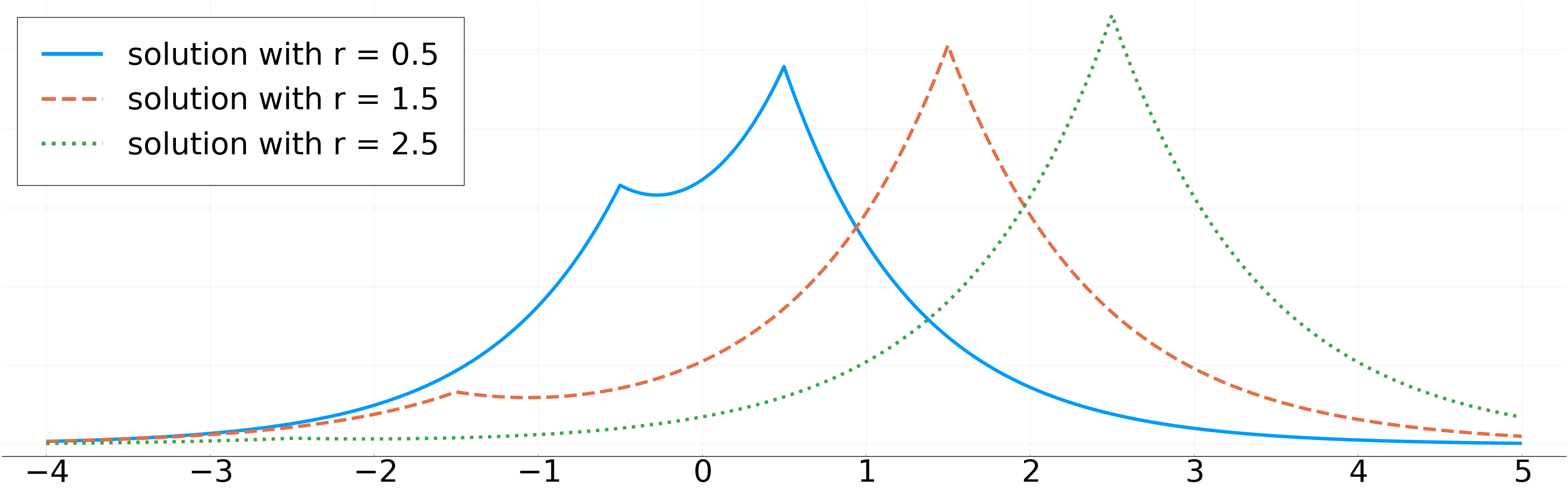
Figure 1: Three example solutions in $\mathcal{M}_{tr}$.

In this section, we present the numerical results obtained with the offline and online algorithms presented above. The code for generating the figures in the following can be found at https://github.com/mdalery/NonLinearReducedBasis. We focus on a system with two nuclei, i.e. $M=2$, and with charges $\mathbf{z}=(0.8,1.1)$ and $\mathbf{r}=(-r,r)$ for $r\in\mathbb{R}_{+}$. For the training set, the $r$’s are equally distributed on the interval $[0.5,3]$ with $\sharp\mathcal{M}_{tr}=251$. On Figure 1, we plot the exact solutions for three examples, namely $r=0.5,1.5,2.5$.

5.1 Offline phase

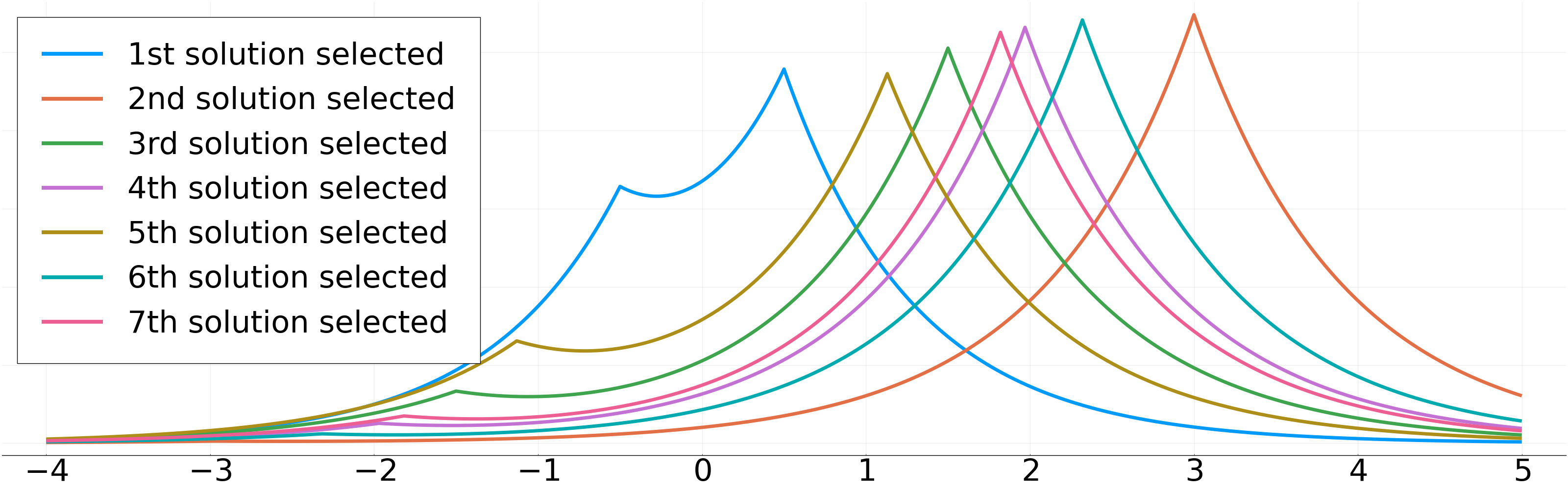
Figure 2: First seven elements selected in the reduced basis in the offline phase.

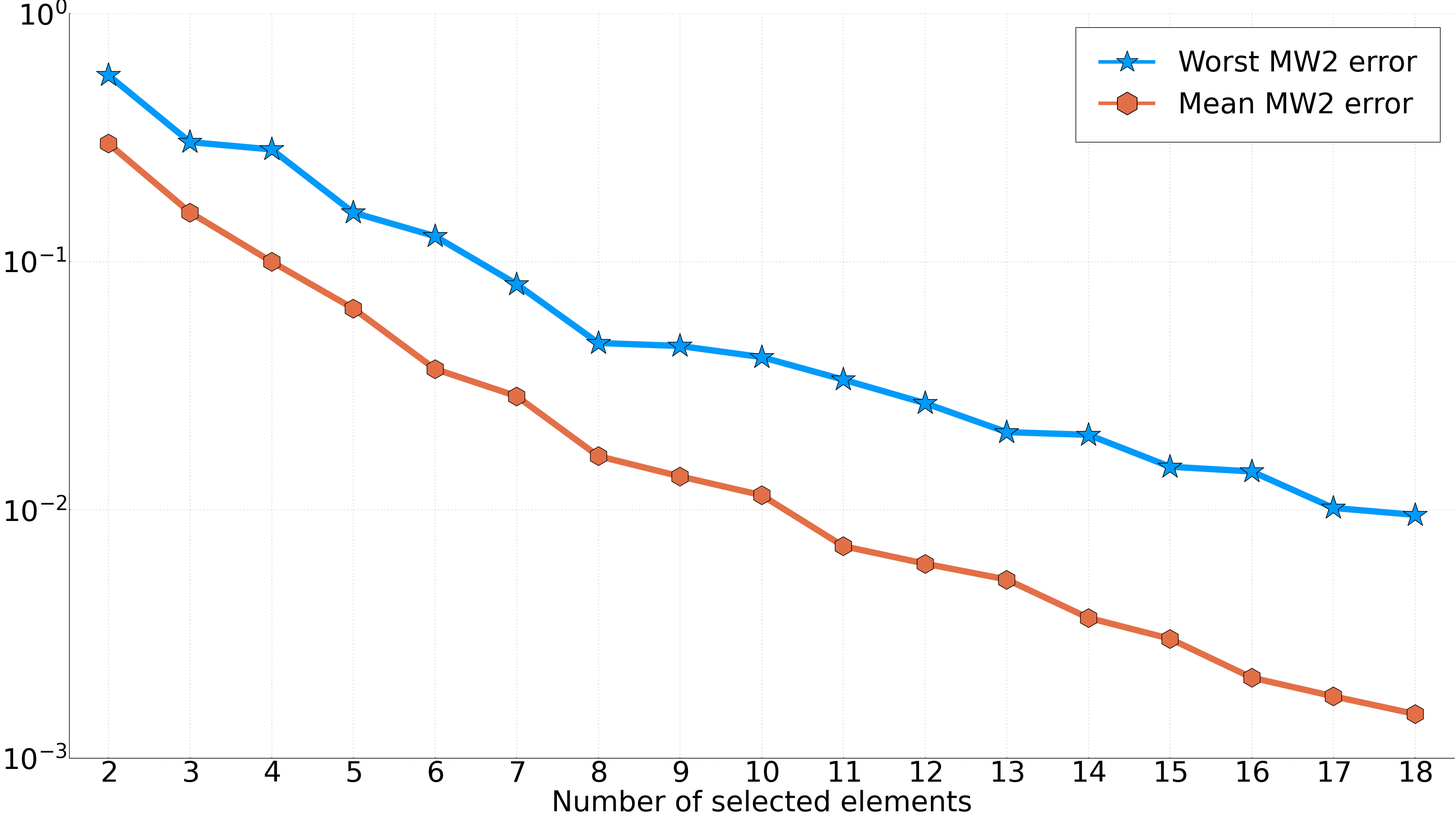
Figure 3: Decay of the projection error in the offline phase.

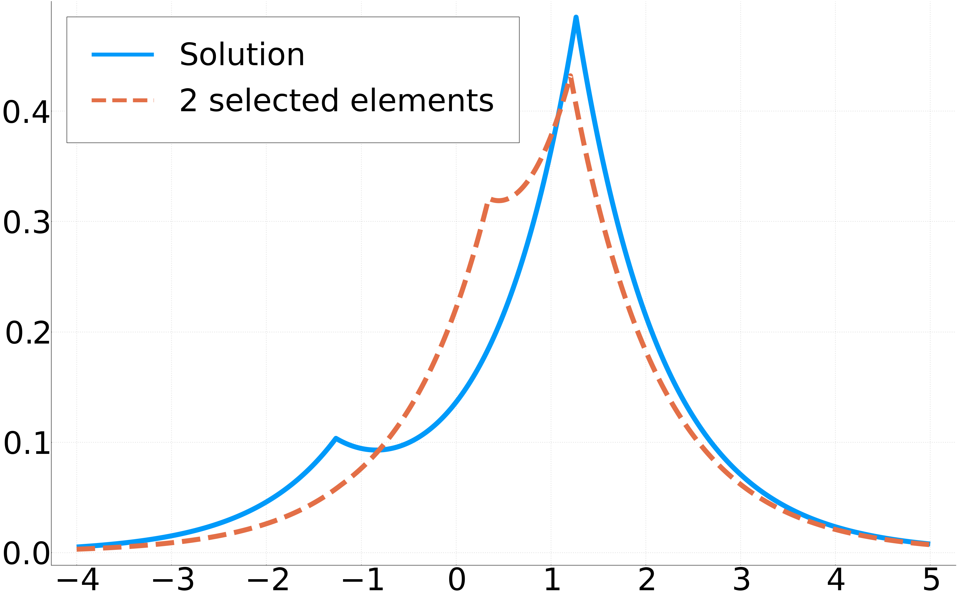
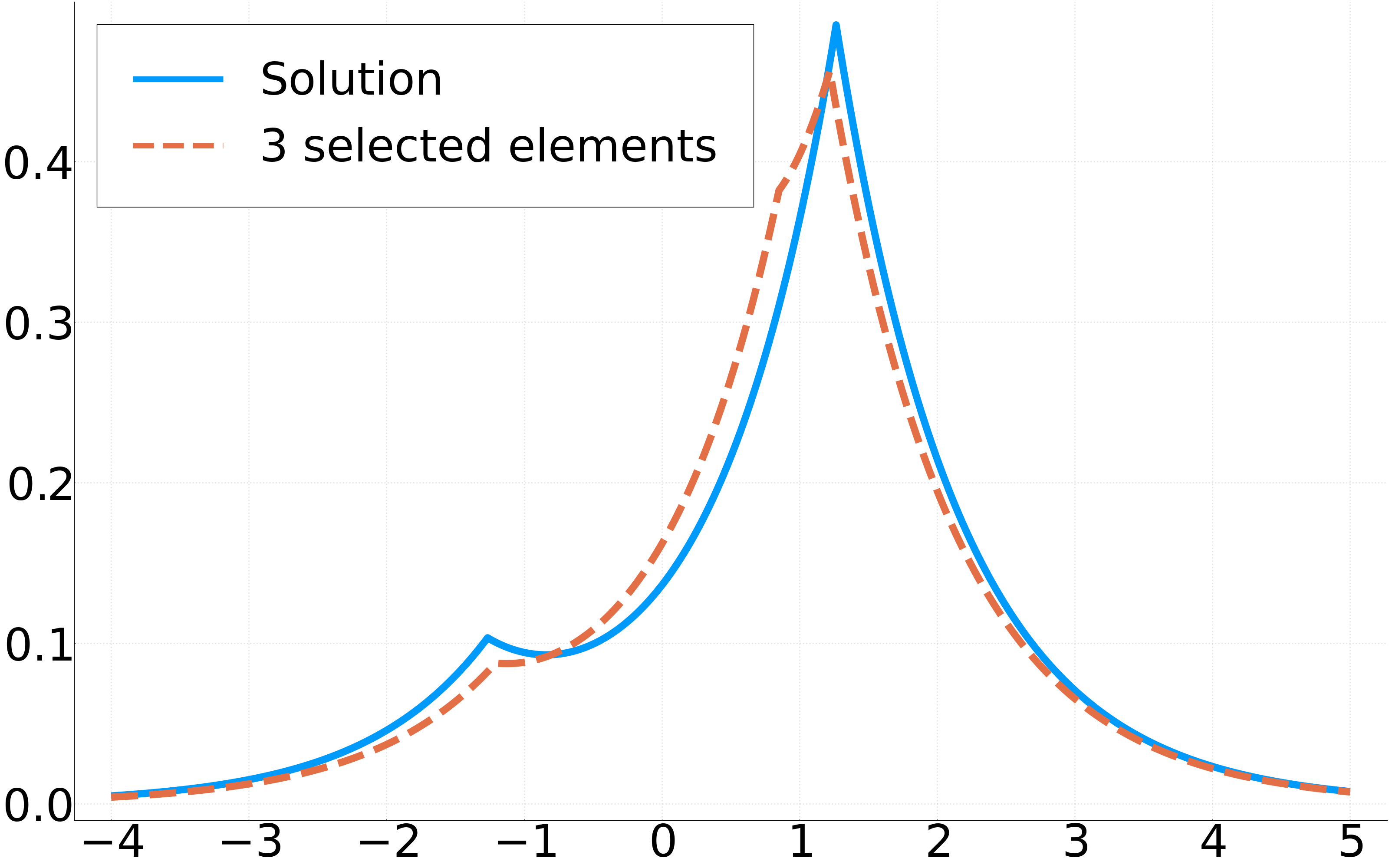
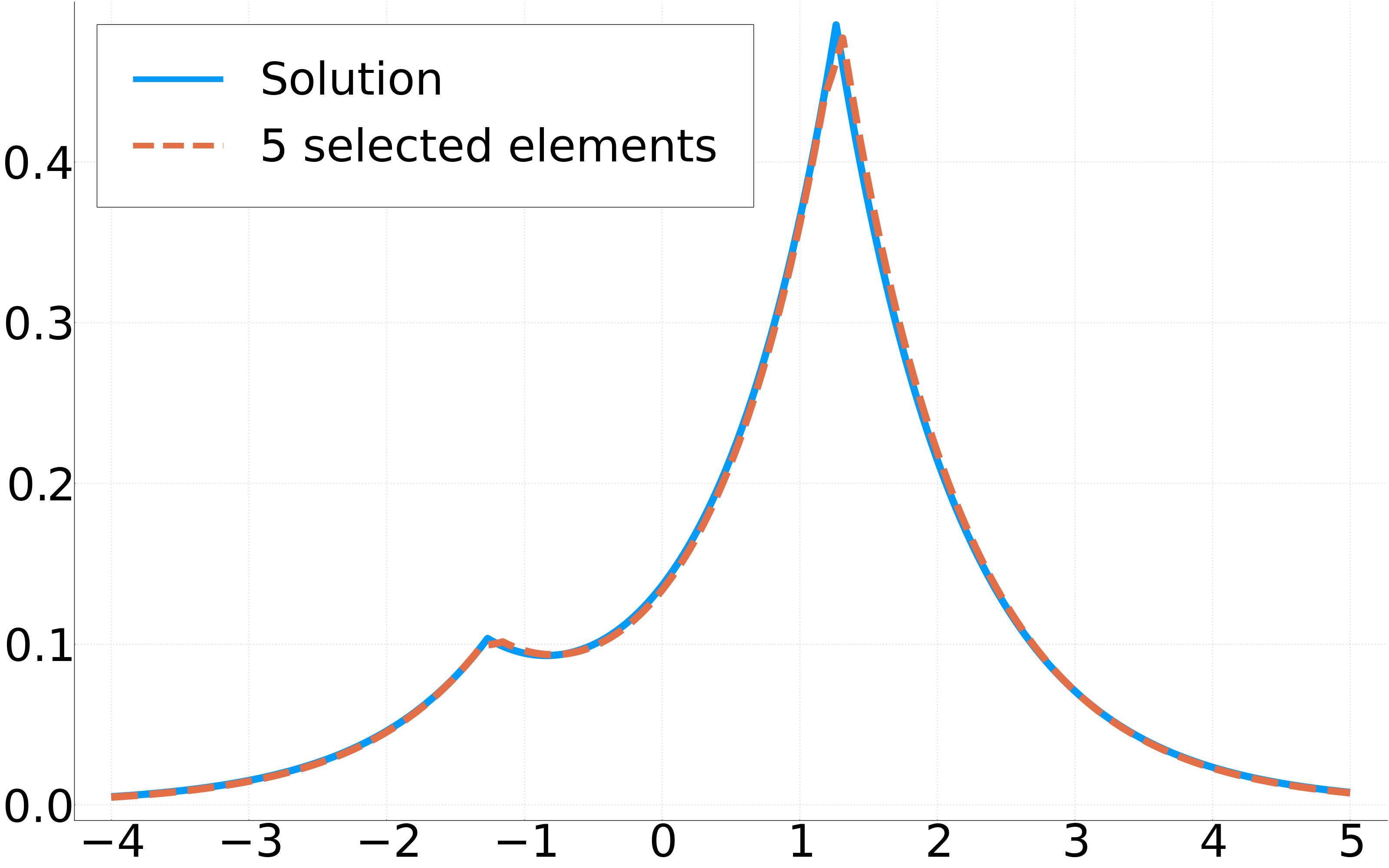
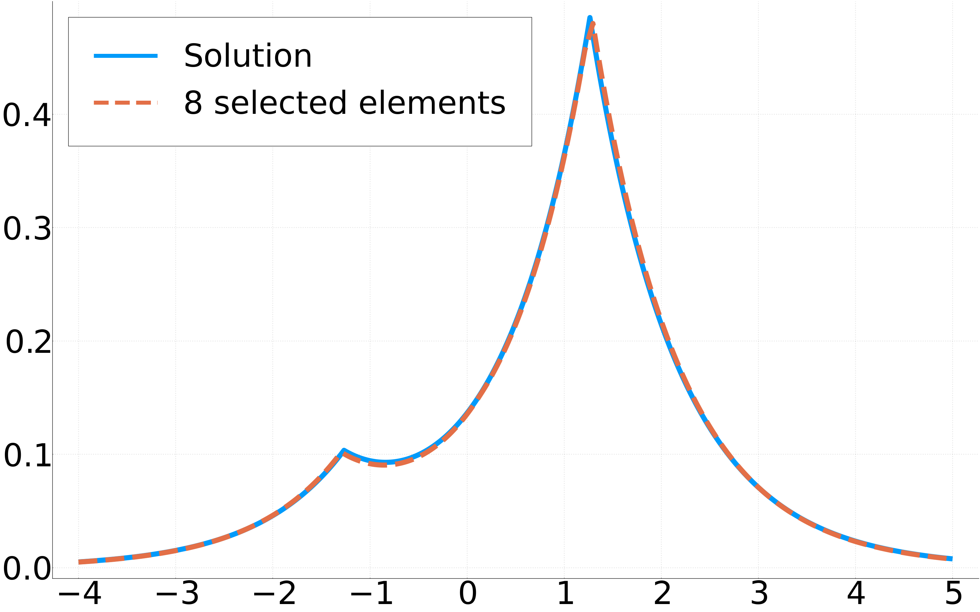
Figure 4: Example of projections on bases with 2,3,5, and 8 elements for $r=1.266$.

We now present the results obtained by running the offline algorithm presented in Section 4.1. We present in Figure 2 the 7 first selected snapshots. We observe that the two first selected snapshots correspond to the extreme parameters $0.5$ and $2.5$, then the next ones are relatively well distributed across the parameter space. In Figure 3, we plot the decrease of the projection error in $\mathrm{MW}_{2}$-norm over the training set. We provide both the mean error on the training set and the maximum error. We observe that this projection error decreases very fast and seems exponentially decreasing. Moreover, we gain about two orders of magnitude between 2 and 15 added snapshots on the mean error.

In terms of computational cost, the most expensive part is the listing of the vertices of the constraint space (4.3), which increases exponentially with the number of selected snapshots. However, the code can be trivially parallelized, and is indeed running on multicores. Also, in the future, a global optimization solver such as Gurobi could be used instead of the listing of the vertices, possibly loosing the global optimality of the found minimizer but gaining a lot in computational efficiency.

In Figure 4, we provide a few examples of projection on the reduced basis for a snapshot with parameter $r=1.266$, which is in $\mathcal{M}_{\mathbf{z}}$ but not in the training set $\mathcal{M}_{tr}$. We observe that the projections cannot be visually distinguished from the exact solution already when the reduced basis contains only 5 elements.

5.2 Online phase

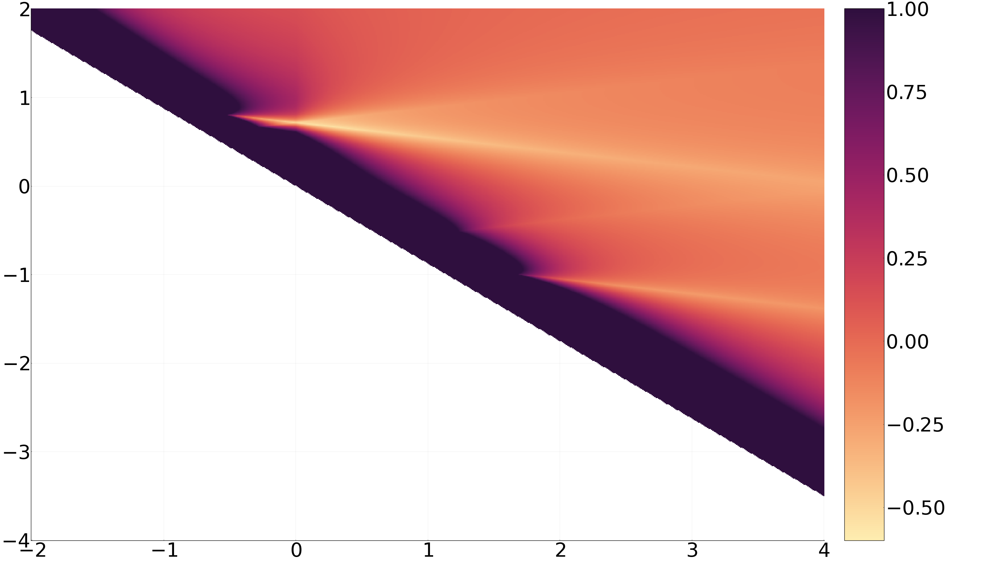
Figure 5: Heatmap of an energy functional (for $r=2.15$) at barycenters between first two selected elements.

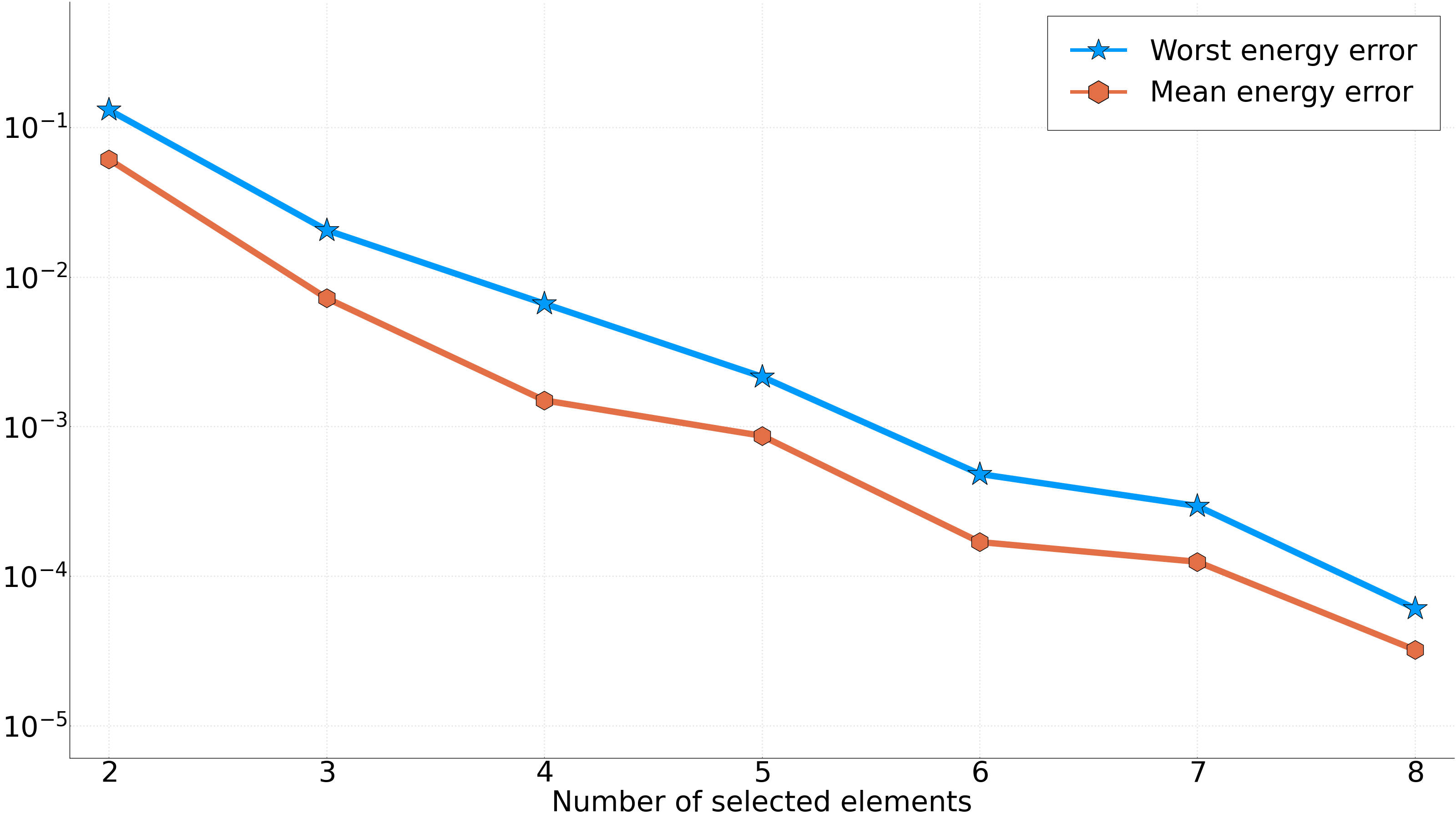
Figure 6: Decay of the energy error in the online phase for 51 equally distributed elements for $r\in[0.5,3]$.

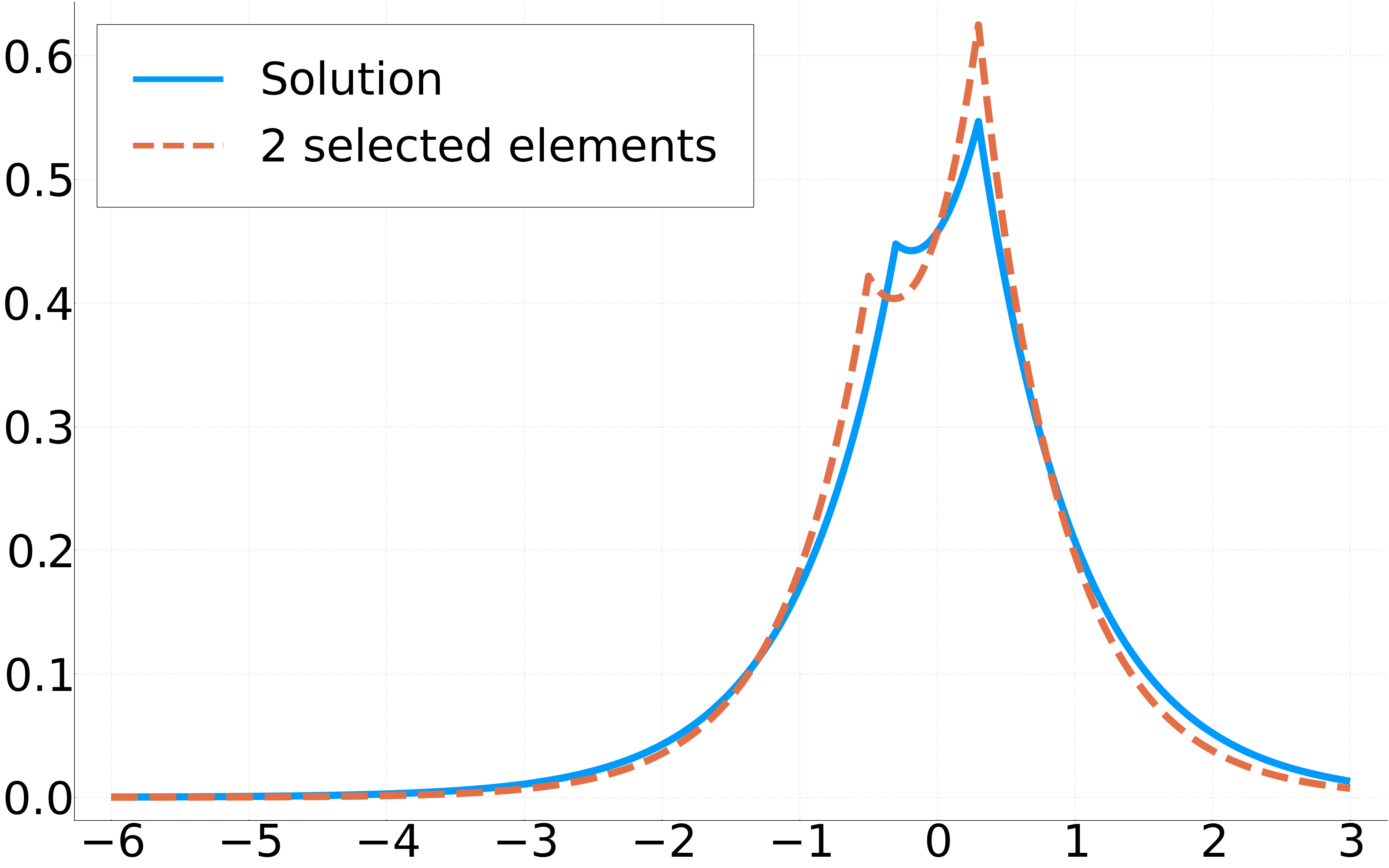
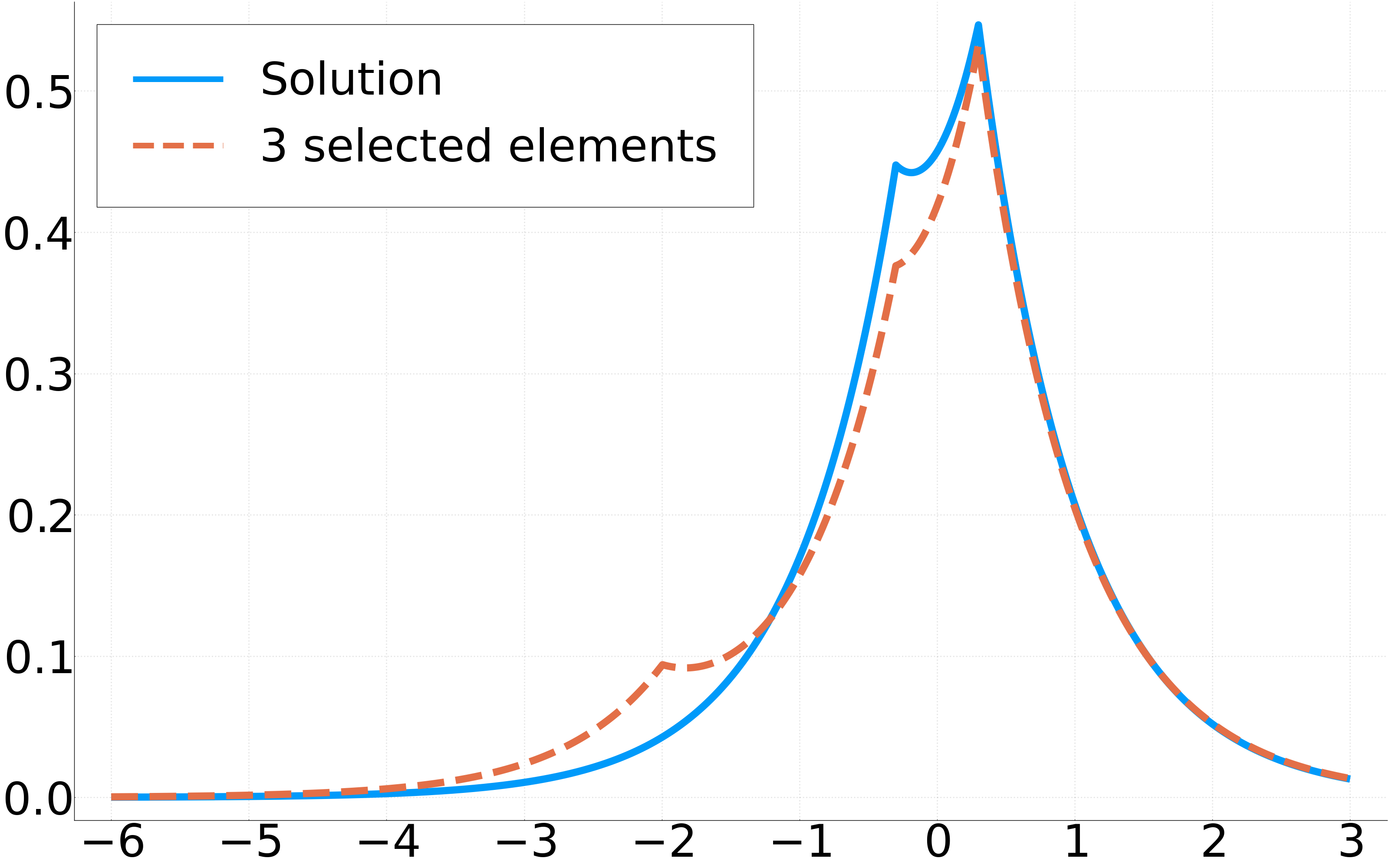
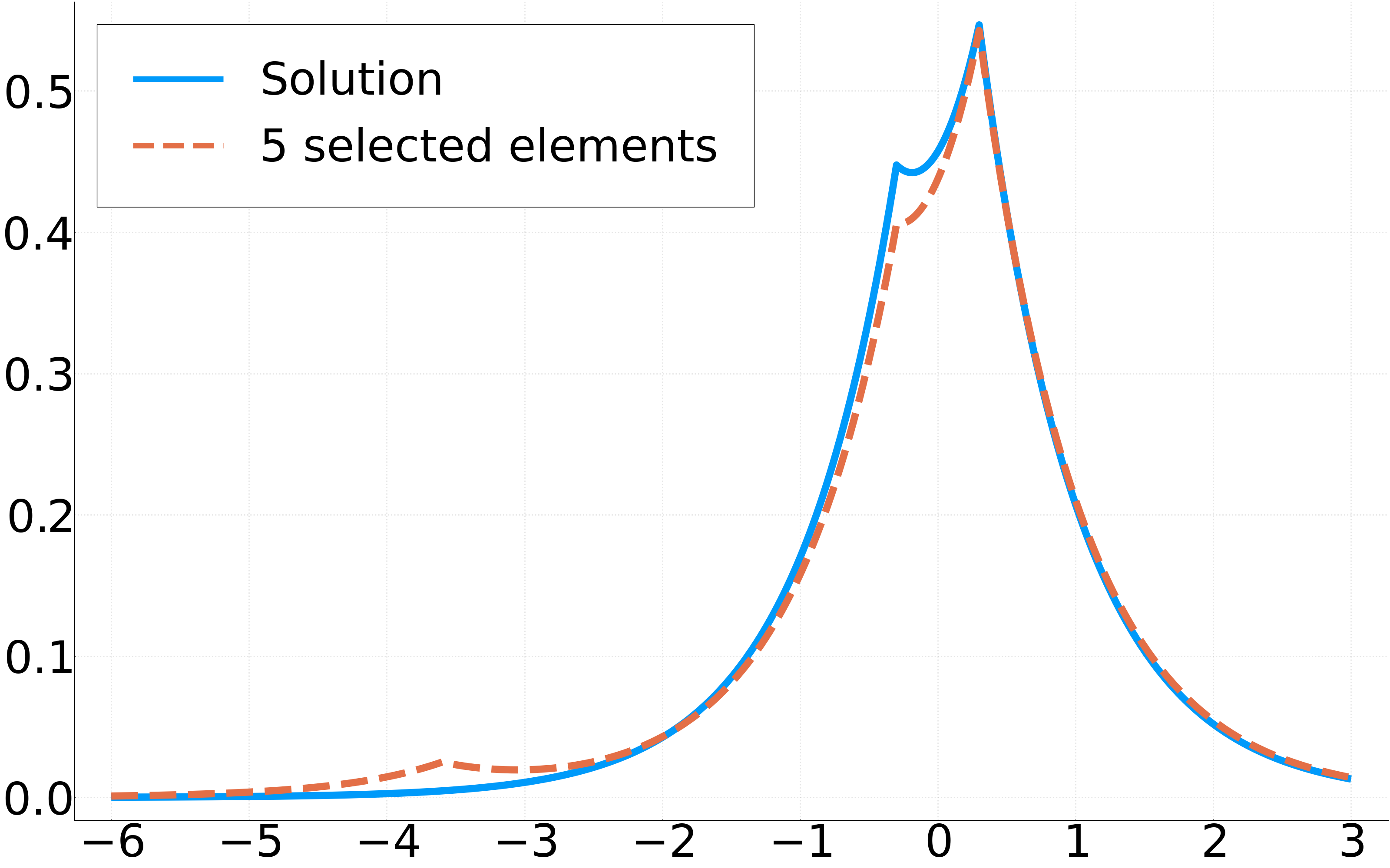
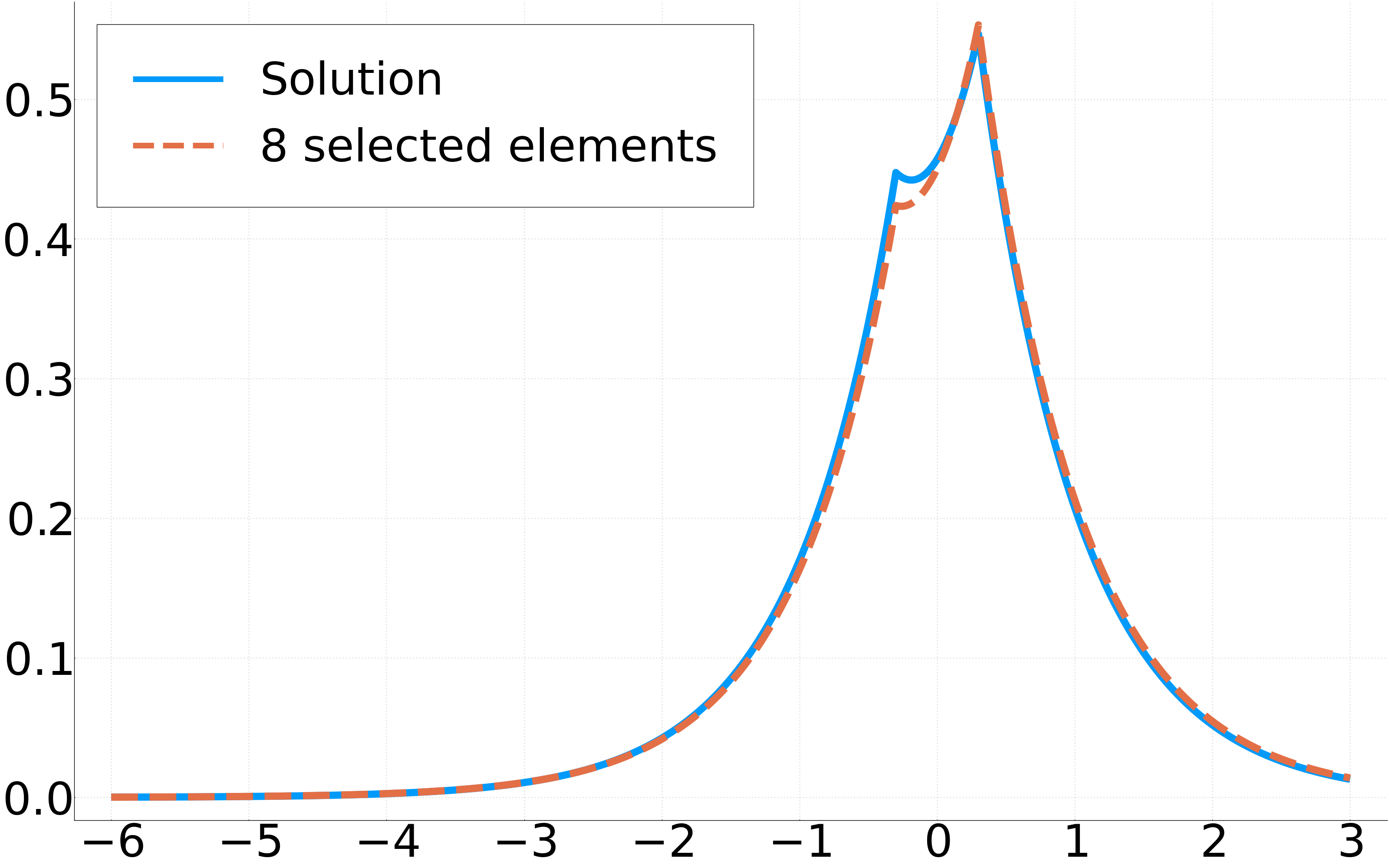
Figure 7: Extrapolation: example of energy projections for $r=0.3$.

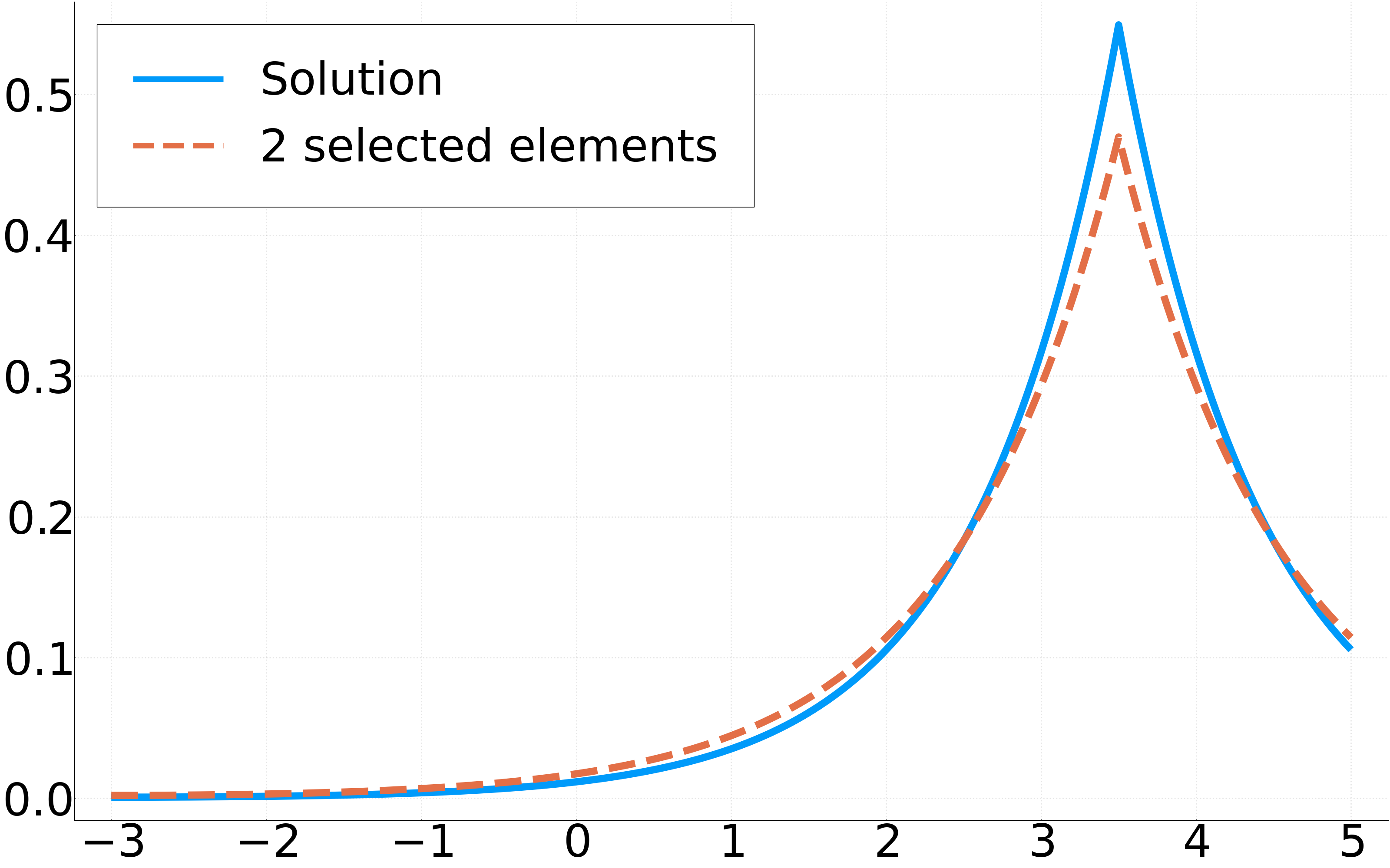
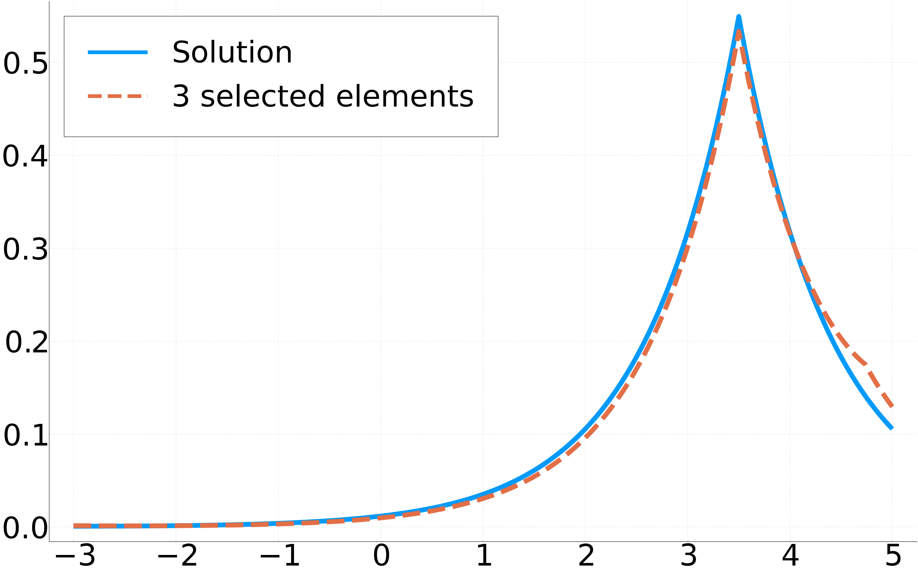
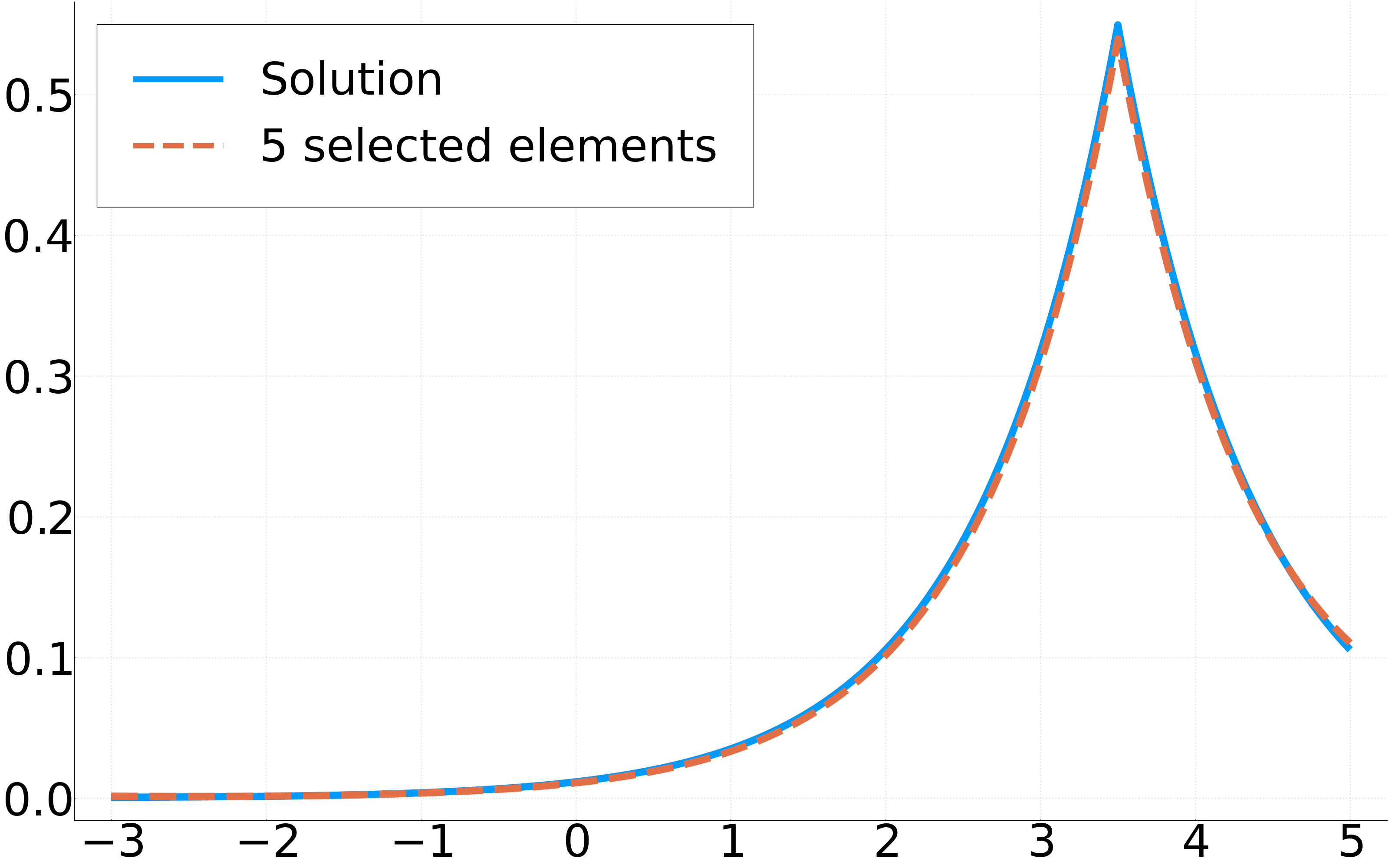
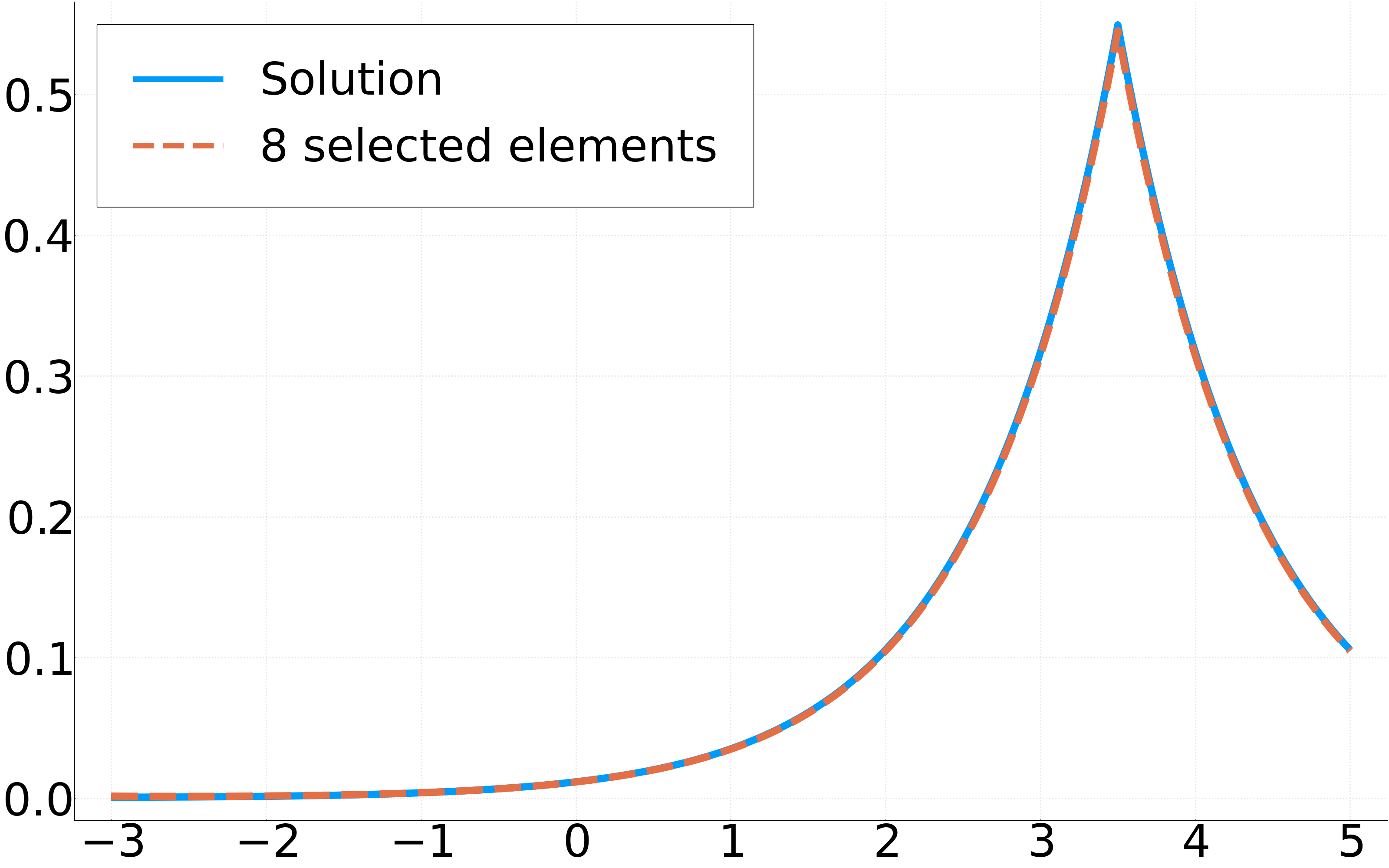
Figure 8: Extrapolation: example of energy projections for $r=3.5$.

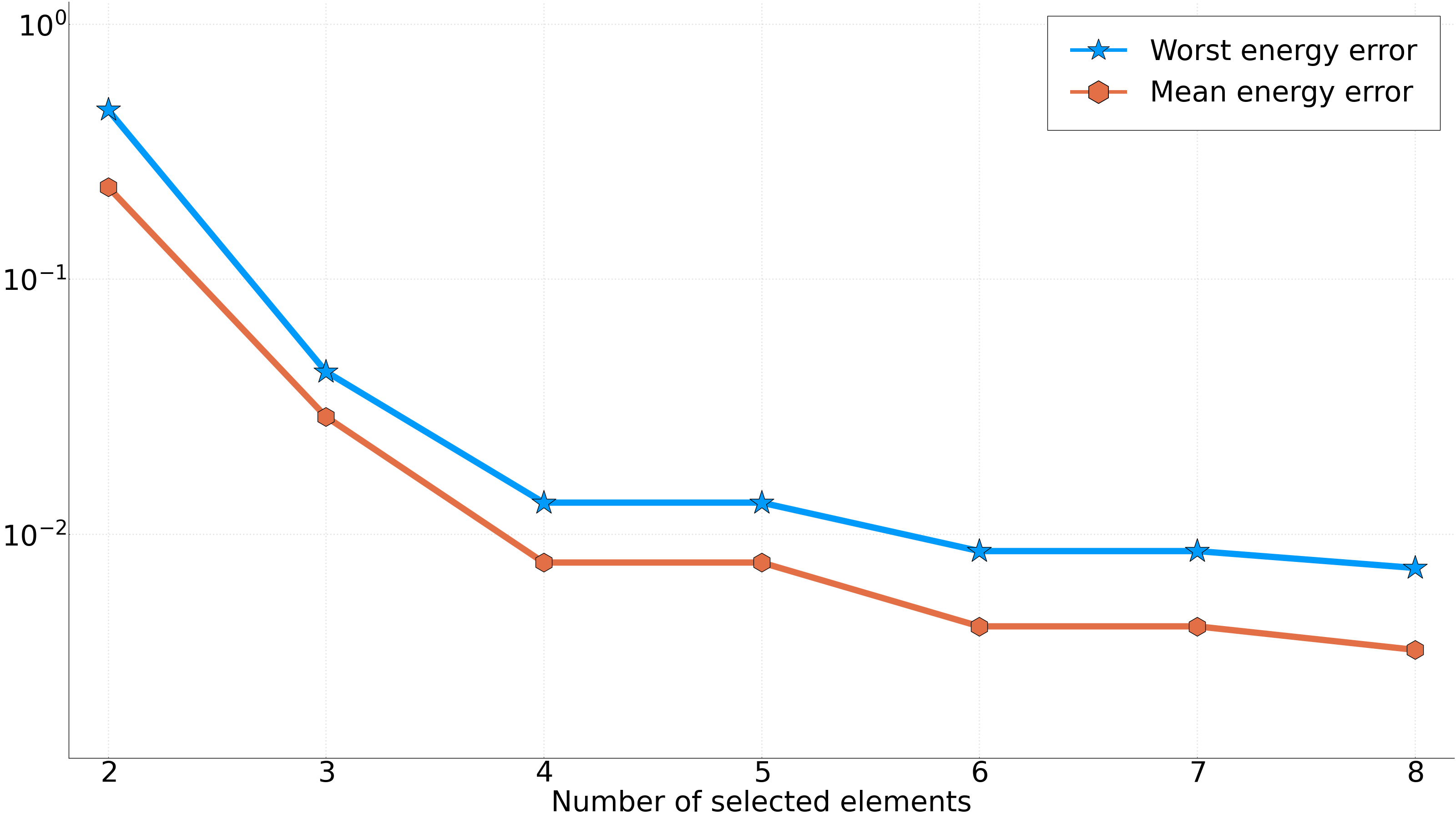
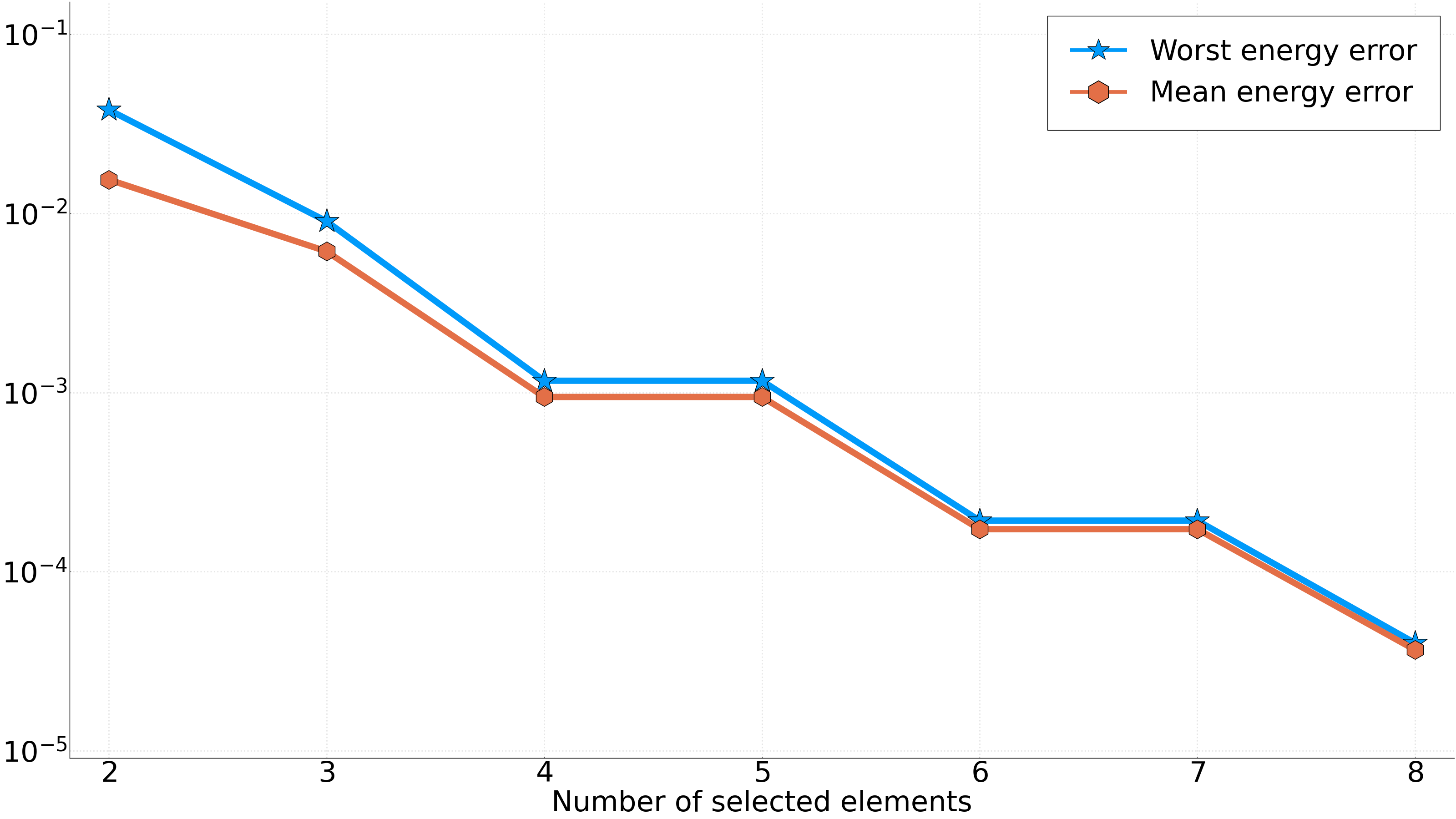
Figure 9: Extrapolation: (Left) Decay of the energy error over a set of $17$ equally distributed elements for $r=0,\dots,0.48$, (Right) Decay of the energy error over a set of $21$ equally distributed elements for $r\in[3.05,\dots,4]$.

In this section we provide results on the online optimization algorithm. First, recall that the energy minimization problem (4.6) is a global optimization problem so that Algorithm 3 may not necessarily return the global minimizer of the problem, possibly overestimating the presented error results compared to the exact ones. In practice, the parameters of Algorithm 3 were chosen as follows. We used a $L=2000$ elements Sobol sequence covering the set $B_{N}=[-2,2]^{N}\cap\Omega_{N}$ as starting points $\bm{\lambda}_{1},\dots,\bm{\lambda}_{L}$.

In Figure 5 we plot an example of energy landscape $\bm{\lambda}\mapsto E_{\mathbf{r},\mathbf{z}}\left(\overline{\mathrm{Bar}}^{\bm{\lambda}}_{\mathrm{MW}_{2}}(m^{1},m^{2})\right)$ heatmap with $\mathbf{z}=(0.8,1.1)$ and $\mathbf{r}=(-r,r)$ for $r=2.15$, where $m^{1}$ and $m^{2}$ are the first two selected snapshots in the offline phase (see Figure 2). The white part corresponds to the outside of the domain $\Omega_{2}$. We already observe several local minima. Moreover, the energy is nonsmooth due to the absolute values appearing in the formula, see Remark 4.3 for more information on the smoothing technique.

We now provide the plot of the error in energy as a function of the number of selected snapshots in Figure 6. We provide both the maximum error and the mean error over a test set of $51$ equally distributed elements for $r\in[0.5,3]$. We observe that the energy maximum error decreases by three orders of magnitude from 2 to 8 snapshots, which is particularly encouraging. Adding more elements in the reduced basis does not seem to improve significantly the results. This may either be due to the increasing difficulty of solving the global optimization problem in larger dimension, but also to the smoothing of the energy functional that is used to avoid convergence problems.

Finally, we provide extrapolation examples. On Figures 7 and 8, we show the projection of the solution on the reduced basis for 2,3,5, and 8 snapshots. We observe that 8 snapshots seems sufficient to obtain a satisfactory barycenter projection of the exact solution onto the reduced basis. More generally, we plot on Figure 9 (Left) the decay of the online error on $17$ equally distributed elements ranging from $r=0$ to $r=0.48$. On Figure 9 (Right), we plot the energy online error on $21$ equally distributed elements with $r=3.05,\dots,4$. We observe that we obtain very accurate results with only a few snapshots in the reduced basis, although the solutions are not in the parameter range of the training set, showing the nice extrapolation capabilities of the method.

6 Conclusion

In this work, we have focused our attention on a one-dimensional parametrized toy problem, which is insightful in terms of the difficulties faced by standard model-order reduction methods to accelerate the resolution of parametrized electronic structure problems. We proved that the linear Kolmogorov $n$-width of solution sets for this equation decays at a slow algebraic rate with respect to $n$. We prove that modified Kolmogorov widths, based on optimal transport tools, in particular Wasserstein mixture distances, decay much faster. Motivated by this result, we proposed a modified greedy algorithm, precisely based on mixture Wasserstein distances and corresponding barycenters, which gives highly encouraging results. Our aim is now to export the ideas and concepts of the present work in order to build efficient reduced-order models for realistic parametrized electronic structure problems in a forthcoming work.

Acknowlegments

The authors thank Alexandre Nou for pointing out the Paley–Wiener results linked to the proof presented in Appendix. They also thank Christoph Ortner for interesting discussions.

This project has received funding from the European Research Council (ERC) under the European Union’s Horizon 2020 research and innovation programme (grant agreement EMC2 No 810367). This work was supported by the French ‘Investissements d’Avenir’ program, project Agence Nationale de la Recherche (ISITE-BFC) (contract ANR-15-IDEX-0003). GD was also supported by the Ecole des Ponts-ParisTech. GD aknowledges the support of the region Bourgogne Franche-Comté. VE acknowledges support from the ANR project COMODO (ANR-19-CE46-0002).

Appendix

Proof 6.1 (Proof of Lemma 3.5).

Using the definition  of the kernel $K$ and rearranging the integrals we remark that, for all $k,l\in\mathbb{N}^{*}$,

$$\langle\varphi_{k},T_{K}\varphi_{l}\rangle =\int_{-R}^{R}\left(\int_{-R}^{R}u_{r}(x)\cos(a_{k}x)\mathrm{d}x\right)\left(\int_{-R}^{R}u_{r}(y)\cos(a_{l}y)\mathrm{d}y\right)\mathrm{d}r$$

$$=\langle T_{S}\cos(a_{k}\cdot),T_{S}\cos(a_{l}\cdot)\rangle,$$

where $T_{S}$ is the compact and self-adjoint operator defined by

(6.1) $$T_{S}:\begin{array}[]{ccc}\mathrm{L}^{2}(-R,R)&\longrightarrow&\mathrm{L}^{2}(-R,R)\\ \varphi&\longmapsto&\displaystyle\left(r\mapsto\int_{-R}^{R}u_{r}(x)\varphi(x)\mathrm{d}x\right).\end{array}$$

The self-adjointness of $T_{S}$ stems from the fact that $u_{r}(x)=u_{x}(r)$ for all $(x,r)\in(-R,R)$. Similarly, it holds that for all $k,l\in\mathbb{N}^{*}$,

$$\langle\varphi_{k},T_{K}\psi_{l}\rangle=\langle T_{S}\varphi_{k},T_{S}\psi_{l}\rangle\quad\mbox{ and }\quad\langle\psi_{k},T_{K}\psi_{l}\rangle=\langle T_{S}\psi_{k},T_{S}\psi_{l}\rangle.$$

For $k\in\mathbb{N}^{*}$, we now compute $T_{S}\cos(a_{k}\cdot)$:

(6.2) $$T_{S}\cos(a_{k}\cdot)(r)=\frac{z}{2}\left(\int_{-R}^{r}e^{z(x-r)}\cos(a_{k}x)\mathrm{d}x+\int_{r}^{R}e^{-z(x-r)}\cos(a_{k}x)\mathrm{d}x\right)$$

We compute the two integrals using two integrations by parts. First

$$I^{-}(r) :=\int_{-R}^{r}e^{z(x-r)}\cos(a_{k}x)\mathrm{d}x$$

$$=\frac{1}{a_{k}}\left[\sin(a_{k}x)e^{z(x-r)}\right]_{-R}^{r}-\frac{z}{a_{k}}\int_{-R}^{r}e^{z(x-r)}\sin(a_{k}x)\mathrm{d}x$$

$$=\frac{\sin(a_{k}r)}{a_{k}}+\frac{\sin(a_{k}R)}{a_{k}}e^{-z(R+r)}+\frac{z}{a_{k}^{2}}\left[\cos(a_{k}x)e^{z(x-r)}\right]_{-R}^{r}-\frac{z^{2}}{a_{k}^{2}}I^{-}(r)$$

$$=\frac{\sin(a_{k}r)}{a_{k}}+\frac{z}{a_{k}^{2}}\cos(a_{k}r)+\frac{a_{k}\sin(a_{k}R)-z\cos(a_{k}R)}{a_{k}^{2}}e^{-z(R+r)}-\frac{z^{2}}{a_{k}^{2}}I^{-}(r)$$

$$=\frac{\sin(a_{k}r)}{a_{k}}+\frac{z}{a_{k}^{2}}\cos(a_{k}r)-\frac{z^{2}}{a_{k}^{2}}I^{-}(r),$$

noting that $a_{k}\sin(a_{k}R)-z\cos(a_{k}R)=0$. In the same manner we can consider the other integral $I^{+}(r):=\int_{r}^{R}e^{-z(x-r)}\cos(a_{k}x)\mathrm{d}x=I^{-}(-r)$ to find

$$I^{+}(r)=-\frac{\sin(a_{k}r)}{a_{k}}+\frac{z}{a_{k}^{2}}\cos(a_{k}r)-\frac{z^{2}}{a_{k}^{2}}I^{+}(r).$$

Hence, continuing from (6.2),

$$T_{S}\cos(a_{k}\cdot)(r)=\frac{z}{2}\left(\frac{2z}{a_{k}^{2}}\cos(a_{k}r)-\frac{z^{2}}{a_{k}^{2}}T_{S}\cos(a_{k}\cdot)(r)\right),$$

which means that

$$T_{S}\cos(a_{k}\cdot)(r)=\frac{2z^{2}}{2a_{k}^{2}+z^{3}}\cos(a_{k}r).$$

Similarly, for $k\in\mathbb{N}^{*}$, we now compute $T_{S}\sin(b_{k}\cdot)$:

(6.3) $$T_{S}\sin(b_{k}\cdot)(r)=\frac{z}{2}\left(\int_{-R}^{r}e^{z(x-r)}\sin(b_{k}x)\mathrm{d}x+\int_{r}^{R}e^{-z(x-r)}\sin(b_{k}x)\mathrm{d}x\right)$$

We compute the two integrals using two integrations by parts. First

$$J^{-}(r) :=\int_{-R}^{r}e^{z(x-r)}\sin(b_{k}x)\mathrm{d}x$$

$$=\frac{1}{b_{k}}\left[-\cos(b_{k}x)e^{z(x-r)}\right]_{-R}^{r}+\frac{z}{b_{k}}\int_{-R}^{r}e^{z(x-r)}\cos(b_{k}x)\mathrm{d}x$$

$$=-\frac{\cos(b_{k}r)}{b_{k}}+\frac{\cos(b_{k}R)}{b_{k}}e^{-z(R+r)}+\frac{z}{b_{k}^{2}}\left[\sin(b_{k}x)e^{z(x-r)}\right]_{-R}^{r}-\frac{z^{2}}{b_{k}^{2}}J^{-}(r)$$

$$=-\frac{\cos(b_{k}r)}{b_{k}}+\frac{z}{b_{k}^{2}}\sin(b_{k}r)+\frac{b_{k}\cos(b_{k}R)+z\sin(b_{k}R)}{b_{k}^{2}}e^{-z(R+r)}-\frac{z^{2}}{b_{k}^{2}}J^{-}(r)$$

$$=\frac{-\cos(b_{k}r)}{b_{k}}+\frac{z}{b_{k}^{2}}\sin(b_{k}r)-\frac{z^{2}}{b_{k}^{2}}J^{-}(r),$$

noting that $b_{k}\cos(b_{k}R)+z\sin(b_{k}R)=0$. In the same manner we can consider the other integral $J^{+}(r):=\int_{r}^{R}e^{-z(x-r)}\sin(b_{k}x)\mathrm{d}x=-J^{-}(-r)$ to find

$$J^{+}(r)=\frac{\cos(b_{k}r)}{b_{k}}+\frac{z}{b_{k}^{2}}\sin(b_{k}r)-\frac{z^{2}}{b_{k}^{2}}J^{+}(r).$$

Hence, continuing from (6.3)

$$T_{S}\sin(b_{k}\cdot)(r)=\frac{z}{2}\left(\frac{2z}{b_{k}^{2}}\sin(b_{k}r)-\frac{z^{2}}{b_{k}^{2}}T_{S}\sin(b_{k}\cdot)(r)\right),$$

which means that

$$T_{S}\sin(b_{k}\cdot)(r)=\frac{2z^{2}}{2b_{k}^{2}+z^{3}}\sin(b_{k}r).$$

Hence, for all $k,l\in\mathbb{N}^{*}$, the functions $\varphi_{k}$ and $\psi_{l}$ are eigenvectors of $T_{S}$ with respective distinct eigenvalues $\sigma_{k}=\dfrac{2z^{2}}{2a_{k}^{2}+z^{3}}$ and $\tau_{l}=\frac{2z^{2}}{2b_{k}^{2}+z^{3}}$. Thus, denoting by $\lambda_{k}=\sigma_{k}^{2}$ and by $\mu_{k}=\tau_{k}^{2}$ for all $k\in\mathbb{N}^{*}$, we obtain that $\displaystyle\bigcup_{k\in\mathbb{N}^{*}}\{\lambda_{k},\mu_{k}\}\subset\sigma(T_{K})$ where $\sigma(T_{K})$ is the spectrum of $T_{K}$. It can also be easily checked that $\{\varphi_{k},\psi_{k}\}_{k\in\mathbb{N}^{*}}$ forms an orthogonal family of functions of $L^{2}(-R,R)$.

It remains to prove that ${\rm Span}\{\phi_{k},\psi_{k}\}_{k\in\mathbb{N}^{*}}$ is dense in $L^{2}(-R,R)$. From [12, Theorem 2], it is clear that $(\psi_{k})_{k\in\mathbb{N}^{*}}$ is an orthogonal basis of the set of odd functions of $L^{2}(-R,R)$. From [23], it holds similarly that $(\phi_{k})_{k\in\mathbb{N}^{*}}$ is an orthogonal basis of the set of even functions of $L^{2}(-R,R)$, hence the desired result. In particular, we then have that $\displaystyle\bigcup_{k\in\mathbb{N}^{*}}\{\lambda_{k},\mu_{k}\}=\sigma(T_{K})$.

References

- [1] M. Agueh and G. Carlier, Barycenters in the wasserstein space, SIAM J. Math. Anal., 43 (2011), pp. 904–924.
- [2] P. C. Álvarez-Esteban, E. del Barrio, J. A. Cuesta-Albertos, and C. Matrán, A fixed-point approach to barycenters in wasserstein space, J. Math. Anal. Appl., 441 (2016), pp. 744–762.
- [3] Y. Chen, T. T. Georgiou, and A. Tannenbaum, Optimal transport for gaussian mixture models, IEEE Access, 7 (2018), pp. 6269–6278.
- [4] A. Cohen and R. DeVore, Approximation of high-dimensional parametric PDEs *, Acta Numer., 24 (2015), pp. 1–159.
- [5] A. Cohen, C. Farhat, A. Somacal, and Y. Maday, Nonlinear compressive reduced basis approximation for PDE’s, Hal preprint hal-04031976, (2023).
- [6] J. Delon and A. Desolneux, A Wasserstein-Type distance in the space of gaussian mixture models, SIAM J. Imaging Sci., 13 (2020), pp. 936–970.
- [7] M.-H. Do, J. Feydy, and O. Mula, Approximation and structured prediction with sparse wasserstein barycenters, arXiv preprint arXiv:2302.05356, (2023).
- [8] G. Dusson, V. Ehrlacher, and N. Nouaime, A wasserstein-type metric for generic mixture models, including location-scatter and group invariant measures, arXiv preprint arXiv:2301.07963, (2023).
- [9] V. Ehrlacher, D. Lombardi, O. Mula, and F.-X. Vialard, Nonlinear model reduction on metric spaces. application to one-dimensional conservative PDEs in wasserstein spaces, Esaim Math. Model. Numer. Anal., 54 (2020), pp. 2159–2197.
- [10] C. A. Floudas and V. Visweswaran, Quadratic optimization, in Handbook of Global Optimization, R. Horst and P. M. Pardalos, eds., Springer US, Boston, MA, 1995, pp. 217–269.
- [11] W. Gangbo and A. Święch, Optimal maps for the multidimensional Monge-Kantorovich problem, Commun. Pure Appl. Math., (1998).
- [12] J. Hammersley, A non-harmonic Fourier series, Acta Mathematica, 89 (1953), pp. 243–260.
- [13] J. S. Hesthaven, G. Rozza, and B. Stamm, Certified Reduced Basis Methods for Parametrized Partial Differential Equations, SpringerBriefs in Mathematics, Springer, 2016.
- [14] A. Iollo and T. Taddei, Mapping of coherent structures in parameterized flows by learning optimal transportation with gaussian models, J. Comput. Phys., 471 (2022), p. 111671.
- [15] R. Milani, A. Quarteroni, and G. Rozza, Reduced basis method for linear elasticity problems with many parameters, Comput. Methods Appl. Mech. Eng., 197 (2008), pp. 4812–4829.
- [16] M. Nonino, F. Ballarin, G. Rozza, and Y. Maday, Overcoming slowly decaying kolmogorov n-width by transport maps: application to model order reduction of fluid dynamics and fluid–structure interaction problems, arXiv preprint arXiv:1911.06598, (2019).
- [17] M. Ohlberger and S. Rave, Reduced basis methods: Success, limitations and future challenges, arXiv preprint arXiv:1511.02021, (2015).
- [18] D. H. Pham, Galerkin method using optimized wavelet-Gaussian mixed bases for electronic structure calculations in quantum chemistry, PhD thesis, Université Grenoble Alpes, June 2017.
- [19] A. Quarteroni, A. Manzoni, and F. Negri, Reduced Basis Methods for Partial Differential Equations: An Introduction, Springer, Aug. 2015.
- [20] A. Quarteroni, G. Rozza, and A. Manzoni, Certified reduced basis approximation for parametrized partial differential equations and applications, J. Math. Ind., 1 (2011), p. 3.
- [21] F. Romor, G. Stabile, and G. Rozza, Non-linear manifold Reduced-Order models with convolutional autoencoders and reduced Over-Collocation method, J. Sci. Comput., 94 (2023), p. 74.
- [22] G. Rozza, C. N. Nguyen, A. T. Patera, and S. Deparis, Reduced basis methods and a posteriori error estimators for heat transfer problems, ASME 2009 Heat Transfer Summer Conference collocated with the InterPACK09 and 3rd Energy Sustainability Conferences, (2010), pp. 753–762.
- [23] S. Verblunsky, On the roots of a transcendental equation, occurring in the theory of trigonometric series, Math. Z., 61 (1954), pp. 324–335.