MLIC⁺⁺: Linear Complexity Multi-Reference Entropy Modeling for Learned Image Compression

Abstract

Recently, learned image compression has achieved impressive performance. The entropy model, which estimates the distribution of the latent representation, plays a crucial role in enhancing rate-distortion performance. The latent representation contains channel-wise, local spatial, and global spatial correlations. However, existing global context modules rely on computationally intensive quadratic complexity computations to capture global correlations. The quadratic complexity imposes limitations on the potential of high-resolution image coding. Moreover, effectively capturing local, global, and channel-wise contexts with acceptable even linear complexity within a single entropy model remains a challenge. To address these limitations, we propose the Linear Complexity Multi-Reference Entropy Model (MEM⁺⁺). MEM⁺⁺ effectively captures the diverse range of correlations inherent in the latent representation. Specifically, the latent representation is first divided into multiple slices. When compressing a particular slice, the previously compressed slices serve as its channel-wise contexts. To capture local contexts without sacrificing performance, we introduce a novel checkerboard attention module with linear complexity. Additionally, to capture global contexts, we propose the linear complexity attention-based global correlations capturing by leveraging the decomposition of the softmax operation. The attention map of the previously decoded slice is implicitly computed and employed to predict global correlations in the current slice. Based on MEM⁺⁺, we propose image compression model MLIC⁺⁺. Extensive experimental evaluations demonstrate that our MLIC⁺⁺ achieves state-of-the-art performance, reducing BD-rate by $13.39\%$ on the Kodak dataset compared to VTM-17.0 in Peak Signal-to-Noise Ratio (PSNR). Furthermore, MLIC⁺⁺ exhibits linear GPU memory consumption with resolution, making it highly suitable for high-resolution image coding. Code and pre-trained models are available at https://github.com/JiangWeibeta/MLIC.

wei.jiang1999@outlook.com, jiangwei@stu.pku.edu.cn
rgwang@pkusz.edu.cn

1 Introduction

Due to the rise of social media, tens of millions of images are generated and transmitted on the web every second.

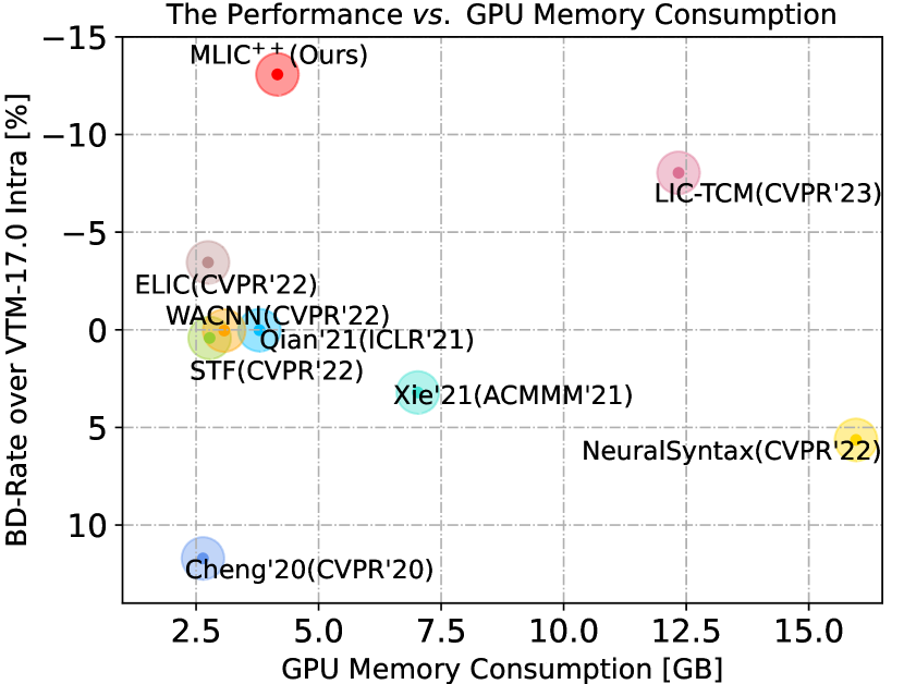
Figure 1: BD-Rate-GPU Memory Consumption during inference on CLIC Professional Valid (Toderici et al., 2020) with 2K resolution. Our MLIC⁺⁺ achieves a better trade-off between performance and GPU memory consumption.

In order to conserve bandwidth, service providers are compelled to seek more efficient and effective image compression methods. Although traditional coding methods like JPEG (Pennebaker & Mitchell, 1992), JPEG2000 (Charrier et al., 1999), AVC (Wiegand et al., 2003), HEVC (Sullivan et al., 2012), and VVC (Bross et al., 2021) have achieved commendable performance, their design relies on manual design for each module. This lack of joint optimization hampers their ability to fully exploit the potential for further advancements in image compression.

Recently, various learned image compression models  (Wu et al., 2022; Guo et al., 2022; Ballé et al., 2017; Theis et al., 2017; Ballé et al., 2018; Minnen et al., 2018; Hu et al., 2020; Ma et al., 2020) have emerged, showcasing impressive performance gains. Notably, certain learned image compression models (Minnen & Singh, 2020; Cheng et al., 2020; Zou et al., 2022; Qian et al., 2020; Xie et al., 2021; He et al., 2022; Jiang et al., 2023b; Chen et al., 2021; Gao et al., 2021; Chen et al., 2022; Koyuncu et al., 2022; Duan et al., 2023; Liu et al., 2023; Jiang et al., 2023a; Fu et al., 2023a; Tang et al., 2023; Chen & Ma, 2023) are already comparable to the advanced traditional method VVC. These models predominantly rely on auto-encoders or variational auto-encoders (Kingma & Welling, 2014), and follow a process that involves transform, quantization, entropy coding, and inverse transform. Entropy coding plays an important role in boosting model performance. An entropy model is utilized to estimate the entropy of the latent representation. A powerful and accurate entropy model usually leads to fewer bits. Expanding contexts of entropy model in learned codecs plays the same role as expanding prediction modes in traditional codecs.

State-of-the-art learned image compression models (Cheng et al., 2020; Minnen & Singh, 2020; Xie et al., 2021; Zhu et al., 2022b; He et al., 2022; Jiang et al., 2023b, a) commonly enhance the entropy model by incorporating a hyper-prior module (Ballé et al., 2018) or a context module (Minnen et al., 2018). These additional modules enable the estimation of conditional entropy and the utilization of conditional probabilities for entropy coding. Context modules usually model probabilities and correlations in different dimensions, including local spatial context module, global spatial context module, and channel-wise context module. However, the current global context modules rely on computationally intensive quadratic complexity computations, which consume huge GPU memories and have slower encoding and decoding speed, imposing limitations on the potential for high-resolution image coding. Furthermore, effectively capturing local, global, and channel-wise contexts with acceptable even linear complexity within a single entropy model remains a challenge. To overcome the aforementioned limitations, we propose a novel linear complexity multi-reference entropy model. This entropy model effectively captures local spatial, global spatial, and channel-wise contexts with linear complexity and can be employed for efficient high-resolution image coding, which is denoted as MEM⁺⁺ to differ from our prior work (Jiang et al., 2023b) presented at ACMMM 2023. Based on MEM⁺⁺, we introduce MLIC⁺⁺, which achieve state-of-the-art performance.

In our approach, the latent representations is divided into multiple slices along the channel dimension. When compressing a particular slice, the previously compressed slices serve as its channel-wise contexts, which are extracted by a channel-wise context module. Local and global context modeling are conducted separately for each slice. The utilization of an auto-regressive local context module (Minnen et al., 2018; Van den Oord et al., 2016) leads to serial decoding, while a checkerboard context module (He et al., 2021) facilitates two-pass parallel decoding by dividing the latent representations into anchor and non-anchor parts. However, it is worth noting that the checkerboard context module may result in a performance degradation of up to $4\%$ (Qian et al., 2022). To address this issue, we propose a novel overlapped checkerboard window attention with linear complexity, which further enhances the local context capturing while retaining two-pass decoding. Some previous methods focus on global context modeling (Qian et al., 2020; Guo et al., 2022), which typically involve quadratic complexity or the utilization of additional bits to store global similarity as side information. Additionally, these global context modules often collaborate with serial local spatial context modules, further increasing the computational complexity. Assuming comparable spatial correlations across different slices, we initially calculate the attention map of the previously decoded $i-1$-th slice in a vanilla approach. This attention map is utilized to predict the global correlations within the $i$-th slice. However, in the vanilla attention mechanism, the softmax operation dictates the order of computation among tensors, where the attention map, product of queries and keys are required to be computed first. To circumvent the quadratic complexity, we employ the decomposition of a softmax operation into two independent softmax operations such that the product of keys and values can be computed first, resulting in linear complexity. The proposed linear complexity attention-based global context modules capture global correlations in an implicit way, as there is no need to directly compute the attention map during training and testing. In addition, we also propose the linear complexity inter-slice global spatial context modules to explore the global correlations in all preceding slices. The linear complexity context allows our model to have a linear relationship between consumed GPU memory and resolution without additional bits, while having the performance gain that comes from the global contexts. Ultimately, we integrate the channel, local, intra-slice, inter-slice global contexts, along with the side information for multi-reference entropy modeling. Our contributions are summarized as follows:

• To address the degradation associated with checkerboard context modeling while preserving the benefits of two-pass decoding, we devise a novel approach called shifted window-based checkerboard attention with linear complexity. This technique enables us to capture local spatial contexts more effectively.

• In order to exploit the global correlations within the latent representations, we divide them into slices and utilize the attention map of the previously decoded slice to predict the global correlations in the current slice. To overcome the quadratic complexity typically associated with the softmax operation in vanilla attention, we decompose it into two independent softmax operations, thereby achieving linear complexity without sacrificing performance. Additionally, we explore the global correlations from previous slices.

• We design linear complexity multi-reference entropy model MEM⁺⁺ which captures local spatial, global spatial and channel contexts, as well as hyper-prior side information. Based on MEM⁺⁺, we propose MLIC⁺⁺, which achieves state-of-the-art performance. The complexity and GPU memory consumption of our model is linear with the resolution. Our proposed MLIC⁺⁺ achieved a better trade-off between complexity and performance as depicted in Fig. 1 .

In comparison to our previous work presented at ACMMM 2023 (Jiang et al., 2023b), MLIC⁺⁺ introduces several significant advancements. The primary distinction lies in the utilization of the proposed linear complexity global spatial context modules without sacrificing performance, as opposed to the quadratic complexity observed in our prior work. This achievement is primarily attributed to the division of the softmax operation, which eliminates the need for a specific order of tensor computation. Our proposed modules incorporate advanced techniques such as learnable position embedding and depth-wise residual bottlenecks (Jiang et al., 2023a). Furthermore, MLIC⁺⁺ captures inter-slice global correlations from all previous slices, in contrast to our previous work (Jiang et al., 2023b), which only considers correlations within the previous one slice. MLIC⁺⁺ exhibits several advantages, including reduced GPU memory consumption and faster encoding and decoding speed. The linear complexity makes our MLIC⁺⁺ highly suitable for high-resolution image coding. These advancements in MLIC⁺⁺ contribute to the field of image compression by offering improved efficiency and performance, while maintaining high-quality compression capabilities.

2 Related Works

2.1 Learned Image Compression

Learned image compression (Ballé et al., 2017; Theis et al., 2017) aims to optimize the trade-off between distortion $\mathcal{D}$ and entropy, where entropy is typically measured in terms of bit-rate $\mathcal{R}$. Large bit-rate usually leads to lower distortion . Lagrange multiplier $\lambda$ is employed to adjust the weight of distortion to control the target bit-rate. The optimization target is

$$\mathcal{L}=\mathcal{R}+\lambda\mathcal{D}.$$ (1)

The fundamental learned image compression framework (Ballé et al., 2017; Theis et al., 2017) is based on the an auto-encoder with a rate penalty. This framework comprises an analysis transform $g_{a}$, a quantization function $Q$, a synthesis transform $g_{s}$ and an entropy model to estimate rates. The process can be formulated as:

$$\boldsymbol{y}=g_{a}(\boldsymbol{x};\theta),\hat{\boldsymbol{y}}=Q(\boldsymbol{y}),\hat{\boldsymbol{x}}=g_{s}(\hat{\boldsymbol{y}};\phi),$$ (2)

where $\boldsymbol{x}$ represents the input image, $g_{a}$ transform the $\boldsymbol{x}$ to compact latent representation $\boldsymbol{y}$. $\boldsymbol{y}$ is quantized to $\hat{\boldsymbol{y}}$ for entropy coding. $\hat{\boldsymbol{x}}$ represents the decompressed image. $\theta$ and $\phi$ are parameters of $g_{a}$ and $g_{s}$. Since quantization is non-differentiable, it can be addressed during training by either adding uniform noise $\mathcal{U}(-0.5,0.5)$ (Ballé et al., 2017, 2018) or using the straight-through estimator (STE) (Theis et al., 2017). In particular, when uniform noise is added, the rate-distortion optimization target in Equation 1 is equivalent to evidence lower bound (ELBO) optimization in variational auto-encoders (Kingma & Welling, 2014). To enhance non-linearity, Generalized Divisive Normalization (GDN) (Ballé et al., 2015) layers or its variants (Qian et al., 2020) are employed. Additionally, self-attention (Vaswani et al., 2017; Liu et al., 2021; Lu et al., 2022; Zou et al., 2022; Liu et al., 2023; Guo et al., 2022), ensemble techniques (Wang et al., 2021), and block partition (Wu et al., 2022) are utilized in transform modules for more compact latent representations. In the basic model, a factorized or a non-adaptive density entropy model is adopted.

In subsequent works, a hyper-prior module (Ballé et al., 2018) is introduced to extract side information $\hat{\boldsymbol{z}}$ from $\boldsymbol{y}$. The hyper-prior model estimates the distribution of $\hat{\boldsymbol{y}}$ from $\hat{\boldsymbol{z}}$. A univariate Gaussian distribution is commonly employed for the hyper-prior. Some works extend it to a mean and scale Gaussian distribution (Minnen et al., 2018), asymmetric Gaussian distribution (Cui et al., 2021), Gaussian mixture model (Cheng et al., 2020; Liu et al., 2020b), and Gaussian-Laplacian-Logistic mixture model (Fu et al., 2023b) for more flexible distribution modeling.

2.2 Context-based Entropy Modeling

Numerous approaches (Minnen et al., 2018; Minnen & Singh, 2020; Qian et al., 2020) have been proposed to improve the accuracy of context modeling in learned image compression. These methods encompass various types of context modules, including local spatial, global spatial, and channel-wise context modules.

Local spatial context modules aim to capture correlations between adjacent symbols. For instance, Minnen et al. (Minnen et al., 2018) utilize a pixel-cnn-like (Van den Oord et al., 2016) masked convolutional layer to capture local correlations between $\hat{\boldsymbol{y}}_{i}$ and symbols $\hat{\boldsymbol{y}}_{<i}$, resulting in serial decoding. He et al. (He et al., 2021) divide latent representation $\hat{\boldsymbol{y}}$ into anchor part $\hat{\boldsymbol{y}}_{a}$ and non-anchor part $\hat{\boldsymbol{y}}_{na}$, employing a checkerboard convolution to extract contexts of $\hat{\boldsymbol{y}}_{na}$ from $\hat{\boldsymbol{y}}_{a}$, thereby achieving two-pass parallel decoding.

On the other hand, some approaches focus on modeling correlations between distant symbols. In (Qian et al., 2020), neighboring left and top symbols serve as bases for computing the similarity between the target symbol and its previous symbols. Guo et al. (Guo et al., 2022) employ the $L2$ distances of symbols to predict global casual dependencies among symbols. In (Kim et al., 2022), the side information is divided into global side information and local side information, introducing additional bits. However, these global context modules are typically combined with serial auto-regressive context modules, which further increase decoding latency. Moreover, existing global context modules (Qian et al., 2020; Guo et al., 2022; Jiang et al., 2023b) often exhibit quadratic complexity, making them challenging to apply in high-resolution image coding. Alternatively, they rely on extra side information (Kim et al., 2022), which increases the bit-rate.

Minnen et al. (Minnen & Singh, 2020) model contexts between channels. $\hat{\boldsymbol{y}}$ is evenly divided to slices. The current slice $\hat{\boldsymbol{y}}^{i}$ is conditioned on previously decoded slices $\hat{\boldsymbol{y}}^{<i}$. To address the uneven distribution of information among slices, an unevenly grouped channel-wise context module is introduced in (He et al., 2022).

While some local and channel-wise context modules (Ma et al., 2021; He et al., 2022; Jiang et al., 2023b) have demonstrated impressive performance, effectively capturing local, global, and channel-wise contexts with acceptable even linear complexity within a single entropy model remains a challenge. Addressing these correlations has the potential to further enhance the performance of image compression models.

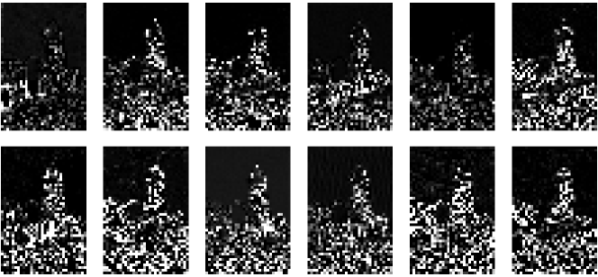
Figure 2: Visualization of channels of latent representation of Kodim19 extracted by Cheng’20 (Cheng et al., 2020) (optimized for MSE, $\lambda=0.0483$) to illustrate channel-wise redundancy.

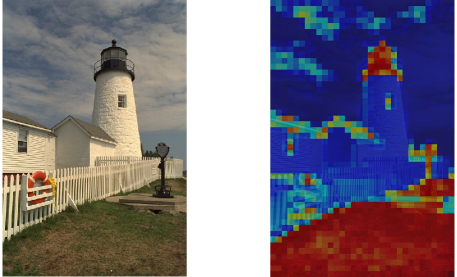
Figure 3: Heatmap of spatial cosine similarity of latent representation of Kodim19 extracted by Cheng’20 (Cheng et al., 2020) (optimized for MSE, $\lambda=0.0483$) to visualize global spatial and local spatial redundancy.

Notations	Explanation
$\boldsymbol{x},\hat{\boldsymbol{x}}$	Input and decoded image
$\boldsymbol{y},\hat{\boldsymbol{y}}$	Non-quantized and quantized latent representation
$\hat{\boldsymbol{y}}^{i}$	The $i$-th slice of $\hat{\boldsymbol{y}}$
$\hat{\boldsymbol{y}}_{ac},\hat{\boldsymbol{y}}_{na}$	Anchor and non-anchor part of $\hat{\boldsymbol{y}}$
$\boldsymbol{z},\hat{\boldsymbol{z}}$	Non-quantized and quantized side information
$g_{ep}$	Entropy parameter module
$\mu,\sigma$	Mean and scale of $\hat{\boldsymbol{y}}$
$g_{a},g_{s}$	Analysis and synthesis transform
$h_{a},h_{s}$	Hyper analysis and synthesis
$g_{ch}$	Channel-wise context module
$g_{lc,ckbd}$	Vanilla checkerboard context module
$g_{lc,attn}$	Shifted Window-based Checkerboard Attention
$g_{gc,intra}$	Intra-slice global spatial context module
$g_{gc,inter}$	Inter-slice global spatial context module
${\boldsymbol{\Phi}}_{h},\boldsymbol{\Phi}_{ch},{\boldsymbol{\Phi}}_{lc}$	Hyper-prior, channel-wise and local spatial context
${\boldsymbol{\Phi}}_{gc,intra}$	Intra-slice global spatial context
${\boldsymbol{\Phi}}_{gc,inter}$	Inter-slice global spatial context
MEM ++	Linear complexity
	multi-reference entropy model
$M,N,S$	Channel number of $\boldsymbol{y}$, $\boldsymbol{z}$, and $\hat{\boldsymbol{y}}^{i}$
$K$	Kernel size of local spatial context module
Q, AE, AD	Quantization, arithmetic encoding and decoding

Table 1: Explanations of notations.

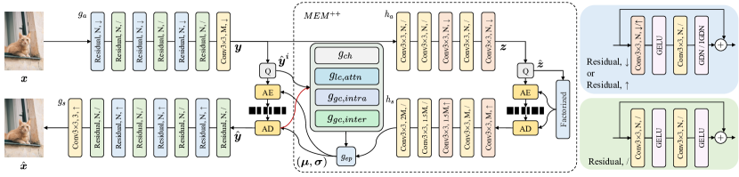
Figure 4: The overall architecture of MLIC⁺⁺. $\downarrow$ means down-sampling. $\uparrow$ means up-sampling. / means stride equals $1$. Red line is the dataflow during decoding. ${\boldsymbol{x}}$ is the input image and $\hat{\boldsymbol{x}}$ is the reconstructed image. $\boldsymbol{y}$ is the latent representation and $\hat{\boldsymbol{y}}$ is the quantized latent representation. $\hat{\boldsymbol{y}}^{i}$ is the $i$-th slice of $\hat{\boldsymbol{y}}$. .

3 Method

3.1 Motivation

According to information theory, the conditional entropy is bounded by the entropy:

$$H(\hat{\boldsymbol{y}})\geq H(\hat{\boldsymbol{y}}|\boldsymbol{ctx}),$$ (3)

where $H$ denotes Shannon entropy, $\boldsymbol{ctx}$ is the context of $\hat{\boldsymbol{y}}$. Exploiting correlations in $\hat{\boldsymbol{y}}$ results in bit savings.

In Fig. 2 and Fig. 3, channel-wise correlations and spatial correlations in latent representation of Kodim19 extracted by Cheng’20 (Cheng et al., 2020) are illustrated.

Fig. 2 visualizes the features of several channels, revealing their significant similarity. However, capturing such correlations poses a challenge for spatial context modules, as they employ the same mask for all channels during context extraction. Consequently, certain correlations may not be fully captured.

In Fig. 3, cosine similarity between each symbol and the symbol in the bottom right corner are visualized. Symbols with the same color exhibit a high degree of correlation. Neighbouring symbols have a very high degree of similarity. This observation emphasizes the necessity of a local context module. Furthermore, a global context module is required to capture the correlations between symbols in the bottom-left corner and those in the bottom-right corner, where the grass features share similarities. Additionally, the complexity of global context capturing should be carefully considered and minimized for high-resolution image coding. The latent representation contains redundancy, indicating the potential for bit savings by modeling such correlations.

However, existing entropy models fail to capture correlations in local spatial, global spatial, and channel domains. Spatial context modules have limited interactions between channels, while channel-wise context modules lack interaction within the current slice. Moreover, extending these models to high-resolution image coding with acceptable even linear complexity is non-trivial. These challenges, along with the potential to enhance rate-distortion performance, motivate us to design a linear complexity multi-reference entropy model. Our proposed linear complexity multi-reference entropy model effectively captures correlations in local spatial, global spatial, and channel domains, while maintaining a modest complexity for high-resolution image coding. Further details on our model are presented in the subsequent sections.

3.2 Overall Architecture

3.2.1 MLIC⁺⁺

The overall architecture of proposed model is illustrated in Fig. 4. This model is named MLIC⁺⁺ to distinguish it from MLIC, and MLIC⁺, which are introduced in our conference version (Jiang et al., 2023b). The architecture of MLIC⁺⁺, as depicted in Fig. 4, incorporates the analysis transform $g_{a}$, synthesis transform $g_{s}$, hyper analysis $h_{a}$, and hyper synthesis $h_{s}$, which are simplified versions of Cheng’20 (Cheng et al., 2020). To reduce complexity, attention modules are removed.

$N$	$M$	$S$	$K$	Entropy Model
$192$	$320$	$32$	$5$	MEM++($g_{lc,attn},g_{ch},g_{gc,intra},g_{gc,inter}$)

Table 2: Settings of MLIC⁺⁺ and MEM⁺⁺.

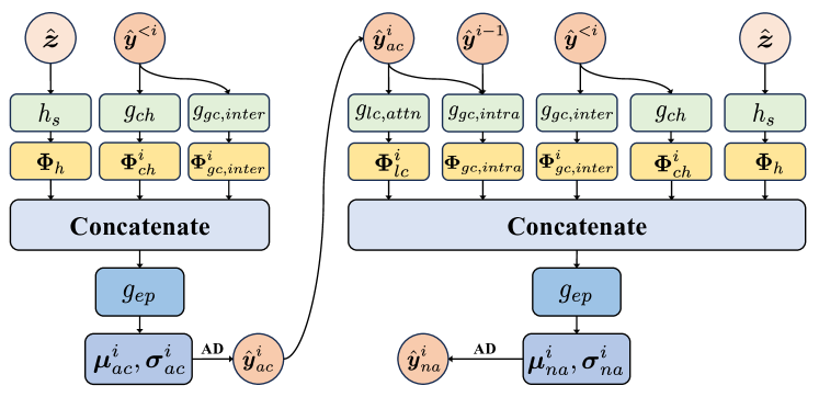
Figure 5: Linear Multi-Reference Entropy Model MEM⁺⁺. The figure illustrates the process of decoding a slice $\hat{\boldsymbol{y}}^{i}$.

The hyper-parameters and settings of MLIC⁺⁺ are presented in Table 2. Same to Minnen et al. (Minnen & Singh, 2020), we adopt mixed quantization, which involves adding uniform noise for entropy estimation and utilizing STE (Theis et al., 2017) to ensure differentiability in the quantization process. Gaussian mean-scale distribution is adopted for entropy estimation. For latent representation $\boldsymbol{y}$, the quantization and estimated rate is formulated as:

$$\hat{\boldsymbol{y}}=\mathrm{STE}(\boldsymbol{y}-\boldsymbol{\mu})+\boldsymbol{\mu},\\$$ (4)

$$\mathcal{R}_{\hat{\boldsymbol{y}}}=\mathbb{E}\left[-\log\int_{-0.5}^{0.5}p({\boldsymbol{y}+\boldsymbol{u}})d\boldsymbol{u}\right],$$ (5)

where $\boldsymbol{\mu}$ is the estimated mean of latent representation $\boldsymbol{y}$, $\boldsymbol{u}\sim\mathcal{U}(-0.5,0.5)$, $\mathcal{R}_{\hat{\boldsymbol{y}}}$ is the estimated rate of $\hat{\boldsymbol{y}}$.

3.2.2 MEM⁺⁺

The proposed linear complexity multi-reference entropy model effectively captures channel-wise, local spatial, and global spatial correlations with linear complexity. The linear complexity entropy model is denoted as MEM⁺⁺ to distinguish it from MEM, and MEM⁺, which are proposed in our conference version (Jiang et al., 2023b). To capture multi-correlations, the proposed MEM⁺⁺ consists of four components: channel-wise context module $g_{ch}$, local spatial context module $g_{lc}$, intra-slice global spatial context module $g_{gc,intra}$, and inter-slice global spatial context module $g_{gc,inter}$. In the channel-wise context module, the latent representation $\hat{\boldsymbol{y}}$ is divided into slices $\{\hat{\boldsymbol{y}}^{0},\hat{\boldsymbol{y}}^{1},\cdots\,\hat{\boldsymbol{y}}^{L}\}$ (Minnen & Singh, 2020) along the channel dimension, $L$ is the number of slices. For the $i$-th slice $\hat{\boldsymbol{y}}^{i}$, the channel-wise context module captures the channel-wise context $\boldsymbol{\Phi}_{ch}^{i}$ from slices $\hat{\boldsymbol{y}}^{<i}$. To capture local spatial correlations, checkerboard pattern (He et al., 2021) is employed, where the latent representation $\hat{\boldsymbol{y}}^{i}$ is divided into anchor part $\hat{\boldsymbol{y}}_{ac}^{i}$ and non-anchor part $\hat{\boldsymbol{y}}_{na}^{i}$. $\hat{\boldsymbol{y}}_{ac}^{i}$ is local-context-free. Local spatial context ${\boldsymbol{\Phi}}_{lc}^{i}$ of $\hat{\boldsymbol{y}}_{na}^{i}$ is captured from $\hat{\boldsymbol{y}}_{ac}^{i}$. We propose Overlapped Window-based Checkerboard Attention $g_{lc,attn}$ for better non-linearity and adaptability to capture local spatial contexts. The global contexts $\boldsymbol{\Phi}_{gc}$ of $i$-th slice are extracted from two dimensions: intra-slice contexts $\boldsymbol{\Phi}_{gc,intra}^{i}$, and inter-slice contexts $\boldsymbol{\Phi}_{gc,inter}^{i}$. We propose Intra-Slice Global Context Module $g_{gc,intra}^{i}$ and Inter-Slice Global Context Module $g_{gc,inter}$ to capture such correlations. Since different slices share the similar global similarity (Jiang et al., 2023b; Guo et al., 2022), the global similarity of $\hat{\boldsymbol{y}}^{i-1}$ is employed to predict the global correlations between $\hat{\boldsymbol{y}}^{i}_{ac}$ and $\hat{\boldsymbol{y}}^{i}_{na}$. The inter-slice global context $\Phi^{i}_{gc,inter}$ are extracted from slices $\hat{\boldsymbol{y}}^{<i}$ via the global similarity of slices $\hat{\boldsymbol{y}}^{<i}$. We introduce these modules in the following sections. The structure of MEM⁺⁺ is illustrated in Table 2. We use Equation 1 as our loss function and the estimated rate can be formulated as: $\mathcal{R}=\mathcal{R}_{\hat{\boldsymbol{z}}}+\sum^{L}_{i=0}\left(\mathcal{R}_{\hat{\boldsymbol{y}}^{i}_{ac}}+\mathcal{R}_{\hat{\boldsymbol{y}}^{i}_{na}}\right)$, where

$$\mathcal{R}_{\hat{\boldsymbol{z}}}=\mathbb{E}\left[-\log\int_{-0.5}^{0.5}p({\boldsymbol{z}+\boldsymbol{u}})d\boldsymbol{u}\right],$$ (6)

$$\mathcal{R}_{\hat{\boldsymbol{y}}^{i}_{ac}}=\mathbb{E}\left[-\log\int_{-0.5}^{0.5}p\left({\boldsymbol{y}}^{i}_{ac}+\boldsymbol{u}|\Phi_{h},\Phi_{ch}^{i},\Phi_{gc,inter}^{i}\right)d\boldsymbol{u}\right],$$ (7)

$$\begin{split}&\mathcal{R}_{\hat{\boldsymbol{y}}^{i}_{na}}=\\ &\mathbb{E}\left[-\log\int_{-0.5}^{0.5}p\left({\boldsymbol{y}}^{i}_{na}+\boldsymbol{u}|\Phi_{h},\Phi_{lc}^{i},\Phi_{ch}^{i},\Phi_{gc,intra}^{i},\Phi_{gc,inter}^{i}\right)d\boldsymbol{u}\right],\end{split}$$ (8)

$\mathcal{R}_{\hat{\boldsymbol{z}}}$ is the rate of side information, $\mathcal{R}_{\hat{\boldsymbol{y}}^{i}_{ac}}$ denotes the rate of the anchor part of $i$-th slice, $\mathcal{R}_{\hat{\boldsymbol{y}}^{i}_{na}}$ denotes the rate of the non-anchor part of $i$-th slice, $\boldsymbol{\Phi}_{h}$ is the hyper-priors extracted by hyper analysis $h_{a}$ and hyper synthesis $h_{s}$.

3.3 Channel-wise Context Module

To extract channel-wise contexts, the latent representation $\hat{\boldsymbol{y}}$ is first evenly divided into multiple slices $\{\hat{\boldsymbol{y}}^{0},\hat{\boldsymbol{y}}^{1},\cdots,\hat{\boldsymbol{y}}^{L}\}$ along the channel dimension. Slice $\hat{\boldsymbol{y}}^{i}$ is conditioned on slices $\hat{\boldsymbol{y}}^{<i}$. A channel context module $g_{ch}$ is employed to squeeze and extract context information from $\hat{\boldsymbol{y}}^{<i}$ when encoding and decoding $\hat{\boldsymbol{y}}^{i}$. $g_{ch}$ consists of three $3\times 3$ convolutional layers. The channel context becomes ${\boldsymbol{{\boldsymbol{\Phi}}}}_{ch}^{i}=g_{ch}(\hat{\boldsymbol{y}}^{<i})$. The channel-wise context module $g_{ch}$ is able to refer to symbols in the same and close position in the previous slices and helps select the most relative channels and extract information beneficial for accurate probability estimation. The channel number of each slice $S$ is a hyper-parameter. Following Minnen et al (Minnen & Singh, 2020), we set $S$ to $32$ and $L$ to $10$ in our model. Following existing methods (Minnen & Singh, 2020; Zou et al., 2022), latent residual prediction (LRP) modules (Minnen & Singh, 2020) are adopted to predict quantization error according to decoded slices and hyper-priors $\boldsymbol{\Phi}_{h}$. Since the channel number of latent representation is freezed during training and inference and the number of slices is quite small, the encoding speed and decoding speed is still fast enough in spite of serial process among slices.

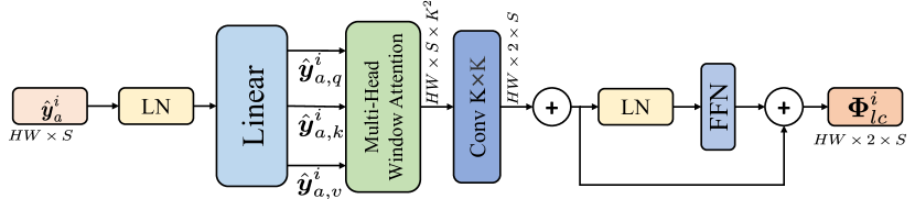
Figure 6: Checkerboard Attention Context Module $g_{lc,attn}$.

3.4 Checkerboard Attention-based Local Context Module

One limitation of CNN-based local context modules is their fixed weights, which restricts their ability to capture content-adaptive contexts. We argue that context-adaptation is essential due to the vast diversity of images. In transformers (Vaswani et al., 2017; Dosovitskiy et al., 2021; Liu et al., 2021), the attention weight is generated dynamically according to the input, which inspires us to design a transformer-based content-adaptive local context module. The local receptive field can be envisioned as a window, where local spatial contexts are captured by dividing the feature map into windows. Since each symbol is most relevant to the symbols around it, we propose to make the divided windows overlapped. To achieve this, we propose the novel checkerboard attention context module $g_{lc,attn}$. The process of $i$-th slice is taken as an example. Assuming the resolution of the latent representation $\hat{\boldsymbol{y}}^{i}$ is $H\times W$, the stride is set to $1$ to divide $\hat{\boldsymbol{y}}^{i}$ into $H\times W$ overlapped windows and the window size is $K\times K$. To extract local correlations, the attention map of each window is computed at first. Same as the convolutional checkerboard context module, interactions between $\boldsymbol{y}_{ac}^{i}$ and $\boldsymbol{y}_{na}^{i}$ and interactions in $\boldsymbol{y}_{na}^{i}$ are not allowed. An example of the attention mask is illustrated in Fig. 7. Importantly, this attention mechanism does not alter the resolution of each window. Subsequently, A $K\times K$ convolutional layer is utilized to fuse local context information and and match the size of the local context with that of $\boldsymbol{y}^{i}$ before feeding it to a feed-forward network (FFN) (Vaswani et al., 2017). The overall process is similar to standard transformer (Vaswani et al., 2017). The process is formulated as:

$${{\hat{\boldsymbol{y}}}^{i}}_{attn}=\textrm{softmax}\left(\frac{{{\hat{\boldsymbol{y}}}^{i}}_{ac,q}\times({{\hat{\boldsymbol{y}}}^{i}}_{ac,k})^{\top}}{\sqrt{S}}+mask\right)\times{{\hat{\boldsymbol{y}}}^{i}}_{ac,v},$$ (9)

$${{\hat{\boldsymbol{y}}}^{i}}_{conv}=\textrm{conv}_{K\times K}({{\hat{\boldsymbol{y}}}^{i}}_{attn}),$$ (10)

$${\boldsymbol{\Phi}}^{i}_{lc}=\textrm{FFN}({{\hat{\boldsymbol{y}}}^{i}}_{conv})+{{\hat{\boldsymbol{y}}}^{i}}_{conv},$$ (11)

where $\hat{\boldsymbol{y}}^{i}_{ac,q},\hat{\boldsymbol{y}}^{i}_{ac,k},\hat{\boldsymbol{y}}^{i}_{ac,v}=\textrm{Embed}(\hat{\boldsymbol{y}}^{i}_{ac})$, $\hat{\boldsymbol{y}}^{i}_{ac}$ is anchor part of $i$-th slice, $mask$ the attention mask, $S$ is the channel number of each slice, FFN is the feed-forward neural network (Vaswani et al., 2017).

Note that our overlapped window-partition is with linear complexity, since the complexity of each window is $O(K^{4})$. The complexity of $g_{lc,attn}$ is $\Omega(K^{4}SL)$, where $L=HW$, $S$ is the channel number of a slice.

3.5 Linear Complexity Intra-Slice Global Context Module

During the decoding process, it is challenging to determine the global correlations between the current symbol and other symbols due to the inherent encoding-decoding consistency. This is because the current symbol is unknown during decoding. One potential solution is to embed the global correlations into the bit-stream, but this approach introduces additional bits, thereby increasing the overall bit-rate. Furthermore, in order to obtain precise global similarity, it is necessary to calculate the similarity between the current symbol and all other symbols, which consumes a significant number of bits and is impractical to employ in real-world scenarios. Consequently, representing global similarity with a limited number of bits or without the need for additional bits becomes a non-trivial task.

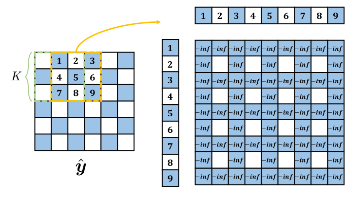
Figure 7: Mask of Shifted Window-based Checkerboard Attention $g_{lc,attn}$. Blue squares are non-anchor part $\hat{\boldsymbol{y}}_{na}$, white squares are anchor part $\hat{\boldsymbol{y}}_{ac}$. Green square and yellow square are two windows.

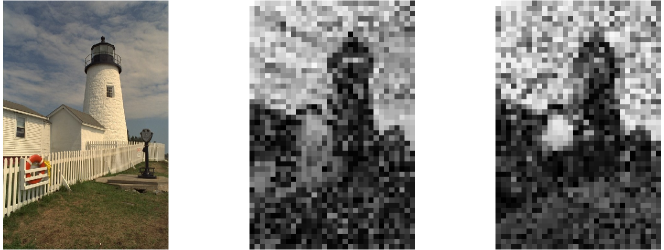
Figure 8: Cosine similarity in the spatial domain of different slices of latent representation of Kodim19 extracted by Cheng’20 (Cheng et al., 2020) (optimized for MSE, $\lambda=0.0483$) to visualize slices share similar global correlations.

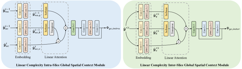
Figure 9: Architectures of Linear Complexity Intra-Slice Global Spatial Context Module and Linear Complexity Inter-Slice Global Spatial Context Module.

In latent representation $\hat{\boldsymbol{y}}\in\mathbb{R}^{L\times C}$, where $L=H\times W$, $C$ is the channel number, each channel contains distinct information, but they can be considered as thumbnails, as depicted in Fig. 2. Notably, the channels exhibit similar global similarities. This is evident from the visualization of cosine similarities between two slices of Cheng’20 (Cheng et al., 2020), as visualized in Fig. 8, where despite differences in magnitude, the global correlations are similar. When decoding the current slice $\hat{\boldsymbol{y}}^{i}\in\mathbb{R}^{L\times S}$, decoded slice $\hat{\boldsymbol{y}}^{i-1}\in\mathbb{R}^{L\times S}$ assists in estimating the global correlations in slice $\hat{\boldsymbol{y}}^{i}$. However, a challenge arises in determining how to estimate these global correlations. While cosine similarity may be useful, it is fixed and may not accurately capture the features. In this regard, attention maps prove to be a suitable choice. The embedding layer is learnable, which make it flexible to adjust the method for global correlations estimation by modifying queries, keys, and values.

First, the vanilla approach is introduced. The process of $i-1$-th slice and the $i$-th slice are taken as an example. When compressing or decompressing $\hat{\boldsymbol{y}}^{i}$, the correlations between anchor part $\hat{\boldsymbol{y}}^{i-1}_{ac}\in\mathbb{R}^{L\times S}$ and non-anchor part $\hat{\boldsymbol{y}}^{i-1}_{na}\in\mathbb{R}^{L\times S}$ of slice $\hat{\boldsymbol{y}}^{i-1}$ are first computed. Because the checkerboard local context module makes anchor visible when decoding non-anchor part, we multiply the anchor part of current slice $\hat{\boldsymbol{y}}^{i}_{a}$ with the attention map between $\hat{\boldsymbol{y}}^{i-1}_{ac}$ and $\hat{\boldsymbol{y}}^{i-1}_{na}$, which is employed as the approximation of global similarities between $\hat{\boldsymbol{y}}^{i}_{ac}$ and $\hat{\boldsymbol{y}}^{i}_{na}$. Due to the local correlations, adjacent symbols have similar global correlations. A $K\times K$ convolutional layer is employed to refine the attention map by aggregating global similarities of adjacent symbols. The process of this Intra-Slice Global Context $g_{gc,inter}$ is parallel and is formulated as:

$$\hat{\boldsymbol{y}}^{i}_{attn}=\underbrace{\textrm{softmax}\left(\frac{{{\hat{\boldsymbol{y}}}^{i-1}}_{na,q}\times\left({{\hat{\boldsymbol{y}}}^{i-1}}_{ac,k}\right)^{\top}}{\sqrt{S}}\right)}_{\textrm{non-negative}}\times\hat{\boldsymbol{y}}^{i}_{ac,v},$$ (12)

$$\hat{\boldsymbol{y}}^{i}_{conv}=\textrm{conv}_{K\times K}(\hat{\boldsymbol{y}}^{i}_{attn}),$$ (13)

$${\boldsymbol{\Phi}}^{i}_{gc,intra}=\textrm{DepthRB}(\hat{\boldsymbol{y}}^{i}_{conv}),$$ (14)

where $\hat{\boldsymbol{y}}^{i-1}_{na,q},\hat{\boldsymbol{y}}^{i-1}_{ac,k}=\textrm{Embedding}\left(\hat{\boldsymbol{y}}^{i-1}\right)$, $\hat{\boldsymbol{y}}^{i}_{ac,v}=\textrm{Embedding}\left(\hat{\boldsymbol{y}}^{i}_{ac}\right)$, Embedding is the embedding layer. Embedding layer consists of a $1\times 1$ convolutional layer and a $3\times 3$ depth-wise convolutional layer. The $3\times 3$ depth-wise convolutional layer is employed for learnable position embedding. This is because the self attention is permutation-invariant and lacks inductive bias. Using a depth-wise convolutional for position embedding does have serval benefits. First, a $3\times 3$ depth-wise convolution is quite light, which has negligible influences on overall complexity. Second, a convolution-based position embedding is flexible for any resolution, due to its translation equivariance. Third, the convolution is able to embed position information because of the zero-padding and the boundary effects (Kayhan & Gemert, 2020; Islam et al., 2019) of images. DepthRB is the depth-wise residual bottleneck (Jiang et al., 2023a) and is employed to enhance the non-linearity.

One drawback of vanilla approach is its quadratic complexity. In Equation 12, the softmax operation specifies the order of tensor calculation. The complexity of ${{\hat{\boldsymbol{y}}}^{i-1}}_{na,q}\times\left({{\hat{\boldsymbol{y}}}^{i-1}}_{a,k}\right)^{\top}$ is $O(L^{2})$. The quadratic complexity leads to huge GPU memory consumption, longer encoding and decoding time as illustrated in Fig. 12, which makes it hard to employ the vanilla approach for high-resolution image coding. In Equation 12, if $\left(\hat{\boldsymbol{y}}^{i-1}_{ac,k}\right)^{\top}\times\hat{\boldsymbol{y}}^{i}_{ac,v}$ is computed first, the overall complexity becomes $O(L)$, which is linear with the resolution. Equation 12 works because $0<\textrm{softmax}\left(\frac{{{\hat{\boldsymbol{y}}}^{i-1}}_{na,q}\times\left({{\hat{\boldsymbol{y}}}^{i-1}}_{ac,k}\right)^{\top}}{\sqrt{S}}\right)<1$. The non-negativity makes it can be treated as a learnable similarity metric. If $\textrm{softmax}\left(\frac{{{\hat{\boldsymbol{y}}}^{i-1}}_{na,q}\times\left({{\hat{\boldsymbol{y}}}^{i-1}}_{ac,k}\right)^{\top}}{\sqrt{S}}\right)\to 0$, ${\hat{\boldsymbol{y}}}^{i-1}_{na,q}$ and ${\hat{\boldsymbol{y}}}^{i-1}_{na,q}$ are near orthogonal. If $\textrm{softmax}\left(\frac{{{\hat{\boldsymbol{y}}}^{i-1}}_{na,q}\times\left({{\hat{\boldsymbol{y}}}^{i-1}}_{ac,k}\right)^{\top}}{\sqrt{S}}\right)\to 1$, ${\hat{\boldsymbol{y}}}^{i-1}_{na,q}$ and ${\hat{\boldsymbol{y}}}^{i-1}_{na,q}$ are very similar. To solve the quadratic complexity, it is necessary to introduce a new operator $\rho$ which avoids the necessity to compute ${{\hat{\boldsymbol{y}}}^{i-1}}_{na,q}\times\left({{\hat{\boldsymbol{y}}}^{i-1}}_{a,k}\right)^{\top}$ first in practice while retaining the non-negativity. Efficient attention operation (Shen et al., 2021) is introduced for non-negativity and linear complexity, which employ the softmax operation on $\hat{\boldsymbol{y}}^{i-1}_{na}$ in row and the softmax operation on $\hat{\boldmath{y}}^{i-1}_{ac}$ in column.

$$\textrm{Attention}=\underbrace{\textrm{softmax}_{2}\left(\hat{\boldsymbol{y}}^{i-1}_{na,q}\right)\textrm{softmax}_{1}\left(\hat{\boldsymbol{y}}^{i-1}_{ac,k}\right)^{\top}}_{\textrm{non-negative}}\hat{\boldsymbol{y}}^{i}_{ac,v}.$$ (15)

The process is illustrated in Equation 15. In Equation 15, $\textrm{softmax}_{2}\left(\hat{\boldsymbol{y}}^{i-1}_{na,q}\right)\textrm{softmax}_{1}\left(\hat{\boldsymbol{y}}^{i-1}_{ac,k}\right)^{\top}$ is employed as the learnable similarity metric, where $0<\textrm{softmax}_{2}\left(\hat{\boldsymbol{y}}^{i-1}_{na,q}\right)<1,0<\textrm{softmax}_{1}\left(\hat{\boldsymbol{y}}^{i-1}_{ac,k}\right)^{\top}<1$, which makes $0<\textrm{softmax}_{2}\left(\hat{\boldsymbol{y}}^{i-1}_{na,q}\right)\textrm{softmax}_{1}\left(\hat{\boldsymbol{y}}^{i-1}_{ac,k}\right)^{\top}<1$. The non-negativity makes $\textrm{softmax}_{2}\left(\hat{\boldsymbol{y}}^{i-1}_{na,q}\right)\textrm{softmax}_{1}\left(\hat{\boldsymbol{y}}^{i-1}_{ac,k}\right)^{\top}$ can be employed as a similarity metric. If $\textrm{softmax}_{2}\left(\hat{\boldsymbol{y}}^{i-1}_{na,q}\right)\textrm{softmax}_{1}\left(\hat{\boldsymbol{y}}^{i-1}_{ac,k}\right)^{\top}\to 0$, ${\hat{\boldsymbol{y}}}^{i-1}_{na,q}$ and ${\hat{\boldsymbol{y}}}^{i-1}_{na,q}$ are near orthogonal. If $\textrm{softmax}_{2}\left(\hat{\boldsymbol{y}}^{i-1}_{na,q}\right)\textrm{softmax}_{1}\left(\hat{\boldsymbol{y}}^{i-1}_{ac,k}\right)^{\top}\to 1$, ${\hat{\boldsymbol{y}}}^{i-1}_{na,q}$ and ${\hat{\boldsymbol{y}}}^{i-1}_{na,q}$ are very similar. The metric is implicit because there is no need to compute $\textrm{softmax}_{2}\left(\hat{\boldsymbol{y}}^{i-1}_{na,q}\right)\textrm{softmax}_{1}\left(\hat{\boldsymbol{y}}^{i-1}_{ac,k}\right)^{\top}$. Since we use softmax operation on $\hat{\boldsymbol{y}}^{i-1}_{na,q}$ and $\hat{\boldsymbol{y}}^{i-1}_{ac,k}$ separately, $\textrm{softmax}_{1}\left(\hat{\boldsymbol{y}}^{i-1}_{ac,k}\right)^{\top}\hat{\boldsymbol{y}}^{i}_{ac,v}$ can be computed first during training and testing. The complexity of it is $O(L)$, which is linear with the resolution. The linear complexity makes it easier to employ the global spatial context module for high-resolution image coding.

3.6 Linear Complexity Inter-Slice Global Context Module

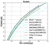
(a)

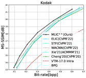
(b)

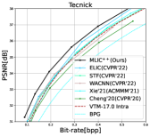
(c)

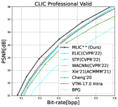
(d)

Figure 10: PSNR-Bit-rate curve and MS-SSIM-Bit-rate curve. MS-SSIM is converted to dB for better visual clarity. Please zoom in for better view.

Because of the global correlations between slices, intra-slice global context module is extended to the inter-slice global context. For a symbol at current slice, the symbol in previous slices is employed at the same position as the approximation of the symbol at current slice, since there are correlations among slices. The correlations among slices or channels are illustrated in Fig. 2 and Fig. 8. This approximation makes the anchor part and non-anchor part benefit from more contexts. The process of $i$-th slice is taken as an example. Same as linear complexity intra-slice global context module, attention mechanism is employed to measure the similarity. To make the inter-slice global context capturing more efficient, the softmax operation in vanilla attention is divided into two independent softmax operations as discussed in Section 3.5. The overall process is

$$\hat{\boldsymbol{y}}^{i}_{attn}=\underbrace{\textrm{softmax}_{2}\left(\hat{\boldsymbol{y}}^{<i}_{q}\right)\textrm{softmax}_{1}\left(\hat{\boldsymbol{y}}^{<i}_{k}\right)^{\top}}_{\textrm{non-negative}}\hat{\boldsymbol{y}}^{<i}_{v},$$ (16)

$$\hat{\boldsymbol{y}}^{i}_{conv}=\textrm{conv}_{K\times K}(\hat{\boldsymbol{y}}^{i}_{attn}),$$ (17)

$${\boldsymbol{\Phi}}^{i}_{gc,inter}=\textrm{DepthRB}(\hat{\boldsymbol{y}}^{i}_{conv}),$$ (18)

where $\hat{\boldsymbol{y}}^{<i}_{q},\hat{\boldsymbol{y}}^{<i}_{k},\hat{\boldsymbol{y}}^{<i}_{v}=\textrm{Embedding}(\hat{\boldsymbol{y}}^{<i})$, Embedding is the embedding layer. Embedding layer consists of a $1\times 1$ convolutional layer and a $3\times 3$ depth-wise convolutional layer. The $3\times 3$ depth-wise convolutional layer is employed for learnable position embedding. DepthRB is the depth-wise residual bottleneck (Jiang et al., 2023a) and is employed to enhance the non-linearity. Since the $\textrm{softmax}_{1}\left(\hat{\boldsymbol{y}}^{<i}_{k}\right)^{\top}\hat{\boldsymbol{y}}^{<i}_{v}$ is computed during training and testing, the similarity metric is implicit and the overall complexity is $O(L)$, which is linear with the resolution.

Methods	Kodak (Kodak, 1993)		Tecnick (Asuni & Giachetti, 2014)		CLIC Professional Valid (Toderici et al., 2020)
	PSNR	MS-SSIM	PSNR	MS-SSIM	PSNR	MS-SSIM
VTM-17.0 Intra (Bross et al., 2021)	$0.00$	$0.00$	$0.00$	$0.00$	$0.00$	$0.00$
Cheng’20 (CVPR’20) (Cheng et al., 2020)	$+5.58$	$-44.21$	$+7.57$	$-39.61$	$+11.71$	$-41.29$
Minnen’20 (ICIP’20) (Minnen & Singh, 2020)	$+3.23$	$-$	$-0.88$	$-$	$-$	$-$
Qian’21 (ICLR’21) (Qian et al., 2020)	$+10.05$	$-39.53$	$+7.52$	$-$	$+0.02$	$-$
Xie’21 (ACMMM’21) (Xie et al., 2021)	$+1.55$	$-43.39$	$+3.21$	$-$	$+0.99$	$-$
Guo’22 (TCSVT’22) (Guo et al., 2022)	$-4.45$	$-45.23$	$-$	$-$	$-$	$-$
LBHIC (TCSVT’22) (Wu et al., 2022)	$-4.56$	$-50.54$	$-$	$-$	$-$	$-$
Entroformer (ICLR’22) (Qian et al., 2022)	$+4.73$	$-42.64$	$+2.31$	$-$	$-1.04$	$-$
SwinT-Charm (ICLR’22) (Zhu et al., 2022b)	$-1.73$	$-$	$-$	$-$	$-$	$-$
NeuralSyntax (CVPR’22) (Wang et al., 2022)	$+8.97$	$-39.56$	$-$	$-$	$+5.64$	$-38.92$
McQuic (CVPR’22) (Zhu et al., 2022a)	$-1.57$	$-47.94$	$-$	$-$	$+6.82$	$-40.17$
STF (CVPR’22) (Zou et al., 2022)	$-2.48$	$-47.72$	$-2.75$	$-$	$+0.42$	$-$
WACNN (CVPR’22) (Zou et al., 2022)	$-2.95$	$-47.71$	$-5.09$	$-$	$+0.04$	$-$
ELIC (CVPR’22) (He et al., 2022)	$-5.95$	$-44.60$	$-9.14$	$-$	$-3.45$	$-$
Contextformer (ECCV’22) (Koyuncu et al., 2022)	$-5.77$	$-46.12$	$-9.05$	$-42.29$	$-$	$-$
Pan’22 (ECCV’22) (Pan et al., 2022)	$+7.56$	$-36.20$	$+3.97$	$-$	$-$	$-$
NVTC (CVPR’23) (Feng et al., 2023)	$-1.04$	$-$	$-$	$-$	$-3.61$	$-$
LIC-TCM (CVPR’23) (Liu et al., 2023)	$-10.14$	$-48.94$	$-11.47$	$-$	$-8.04$	$-$
MLIC (ACMMM’23) (Jiang et al., 2023b)	$-8.05$	$-49.13$	$-12.73$	$-47.26$	$-8.79$	$-45.79$
MLIC+ (ACMMM’23) (Jiang et al., 2023b)	$-11.39$	$-52.75$	$-16.38$	$-53.54$	$-12.56$	$-48.75$
MLIC++ (Ours)	$-13.39$	$-53.63$	$-17.59$	$-53.83$	$-13.08$	$-50.78$

Table 3: BD-Rate $(\%)$ comparison for PSNR (dB) and MS-SSIM. The anchor is VTM-17.0 Intra.

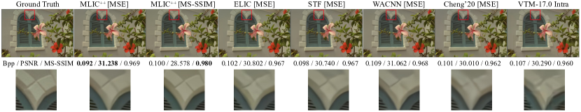
Figure 11: Reconstructions of our proposed MLIC⁺⁺, recent learned image compression models (He et al., 2022; Zou et al., 2022; Xie et al., 2021; Cheng et al., 2020) and VTM-17.0 Intra (Bross et al., 2021). “[MSE]” denotes the model is optimized for MSE and “[MS-SSIM]” denotes the model is optimized for MS-SSIM (Wang et al., 2003). Please zoom in for better view.

4 Experiments

4.1 Implementation Details

4.1.1 Training Dataset

Our training datasets contains $10^{5}$ images with resolutions exceeding $512\times 512$. These images are selected from ImageNet (Deng et al., 2009), COCO 2017 (Lin et al., 2014), DIV2K (Agustsson & Timofte, 2017), and Flickr2K (Lim et al., 2017). To address the existing compression artifacts in JPEG images, we follow the approach of Ballé et al (Ballé et al., 2018) by further down-sampling the JPEG images using a randomized factor. This downsampling process ensures that the minimum height or width of the images falls within the range of 512 to 584 pixels, effectively reducing the compression artifacts.

4.1.2 Training Strategy

MLIC⁺⁺ is built on Pytorch (Paszke et al., 2019) and CompressAI (Bégaint et al., 2020). Following the settings of CompressAI (Bégaint et al., 2020), we set $\lambda\in\{18,35,67,130,250,483\}\times 10^{-4}$ for MSE and set $\lambda\in\{2.4,4.58,8.73,16.64,31.73,60.5\}$ for Multi-Scale Structural Similarity (MS-SSIM) (Wang et al., 2003). The batch size is set to $32$ and models are trained on a single Tesla A100 GPU. Each model is trained with an Adam optimizer with $\beta_{1}=0.9,\beta_{2}=0.999$. We train each model for 2M steps. The learning rate starts at $10^{-4}$ and drops to $3\times 10^{-5}$ at 1.5M steps, drops to $10^{-5}$ at 1.8M steps, and drops to $3\times 10^{-6}$ at 1.9M steps, drops to $10^{-6}$ at 1.95M steps. During training, we random crop images to $256\times 256$ patches during the first $1.2$M steps. To further exploit the effectiveness of global context modules, images are cropped to $512\times 512$ patches during the rest steps. Large patches are beneficial for learning global references. The latent representation can be sparse due to checkerboard partition. A large latent representation makes it more difficult for the model to capture the global contexts and improves the generalization ability of the model across different resolutions.

4.2 Benchmarks and Metrics

To thoroughly assess the generalization capability of the learned image compression models, we conduct performance evaluations on three distinct datasets, including Kodak (Kodak, 1993), Tecnick (Asuni & Giachetti, 2014), CLIC Professional Valid (Toderici et al., 2020).

• Kodak (Kodak, 1993) is selected as a test set for almost all end-to-end image compression models (Ballé et al., 2017; Theis et al., 2017; Ballé et al., 2018; Minnen et al., 2018; Cheng et al., 2020; Minnen & Singh, 2020; Chen et al., 2021; Guo et al., 2022; Wu et al., 2022; Xie et al., 2021; Gao et al., 2021; Chen et al., 2022; Zou et al., 2022; He et al., 2022; Koyuncu et al., 2022; Jiang et al., 2023b; Duan et al., 2023; Liu et al., 2023). It contains 24 raw $768\times 512$ images.

• Tecnick (Asuni & Giachetti, 2014) contains 100 $1200\times 1200$ RGB images, which is used as a test set in many methods (Ballé et al., 2018; Minnen et al., 2018; Xie et al., 2021; Kim et al., 2022; Jiang et al., 2023b, a; Liu et al., 2023; Zhu et al., 2022b; Duan et al., 2023; Pan et al., 2022).

• CLIC Professional Valid (Toderici et al., 2020) is the validation set of 3rd Challenge on Learned Image Compression which contains $41$ images. Image in this dataset contains around $2048\times 1440$ pixels. CLIC Pro Valid is widely used in many recent methods (Cheng et al., 2020; Xie et al., 2021; He et al., 2022; Zou et al., 2022; Liu et al., 2023; Jiang et al., 2023b; Wang et al., 2022; Zhu et al., 2022a; Duan et al., 2023).

We use the Bjøntegaard delta rate (BD-Rate) (Bjontegaard, 2001) to evaluate the performance of learned image compression models.

4.3 Rate-Distortion Performance

4.3.1 Quantitive Results

Rate-distortion curves are presented in Fig. 10. When compared with Cheng’20 (Cheng et al., 2020), our proposed MLIC⁺⁺ can achieve a maximum improvement of $0.5\sim 0.8$ dB in PSNR and achieve a maximum improvement of $0.6$ dB in MS-SSIM in dB. Our MLIC⁺⁺ adopts simplified analysis transform and synthesis transform of Cheng’20 (Cheng et al., 2020), therefore, the improvement of model performance is attributed to our linear complexity multi-reference entropy modeling. Our linear complexity multi-reference entropy models can capture more contexts, which leads to much better rate-distortion performance. The improvement also proves correlations exist in multiple dimensions since Cheng’20 (Cheng et al., 2020) adopts an spatial auto-regressive context module. Compared with ELIC (He et al., 2022), our MLIC⁺⁺ can be up to $0.4$ dB higher at low bit rates in PSNR and $1$ dB higher in MS-SSIM (Wang et al., 2003).

BD-rate reductions are presented in Table 3. When computing BD-rate, VTM-17.0 Intra under YUV444 is employed as anchor. Unofficial weights of ELIC are used to evaluate the rate-distortion performance of ELIC on Tecnick, CLIC Professional Valid. Our MLIC⁺⁺ outperforms our previous MLIC and MLIC⁺ (Jiang et al., 2023b). Our MLIC⁺⁺ reduces BD-rate by $13.39\%$ over VTM-17.0 Intra on Kodak while existing method ELIC only reduces $5.95\%$ BD-rate and LIC-TCM only reduces $10.14\%$ BD-rate on Kodak. Moreover, our MLIC⁺⁺ performs better on high-resolution datasets, such as Tecnick and CLIC Professional Valid. Our MLIC⁺⁺ reduces $17.59\%$ on Tecnick and reduces $13.08\%$ BD-rate on CLIC Professional Valid, which are much better than existing methods. Our MLIC⁺⁺ achieves state-of-the-art performance on all three datasets. The excellent performance of our MLIC⁺⁺ on these datasets also demonstrates the excellent generalization of our MLIC⁺⁺. We highlight the BD-rate for MS-SSIM, our proposed MLIC⁺⁺ reduces about $50\%$ bits compared to VTM-17.0 Intra, which is a large progress in learned image compression.

4.3.2 Qualitive Results

To further demonstrate superiority of our proposed MLIC⁺⁺, we compare our MLIC⁺⁺ with learned image compression models Cheng’20 (Cheng et al., 2020), Xie’21 (Xie et al., 2021), STF (Zou et al., 2022), WACNN (Zou et al., 2022), ELIC (He et al., 2022) and non-neural codec VTM-17.0 Intra (Bross et al., 2021) on perceptual quality. Fig. 11 presents the reconstructions of Kodim07 from Kodak. PSNR value of the image reconstructed by our MLIC⁺⁺ optimized for MSE is $1$dB higher than image reconstructed by VTM-17.0 Intra (Bross et al., 2021). MS-SSIM of the image reconstructed by our MLIC⁺⁺ optimized for MS-SSIM is $0.02$ higher than image reconstructed by VTM-17.0 Intra. The windowsill of reconstructions are cropped to patches for clearer comparisons. The reconstructions of MLIC⁺⁺ have sharper textures retain more details. In terms of visual quality, our MLIC⁺⁺ have significant improvements on rate-perception performance compared to other models.

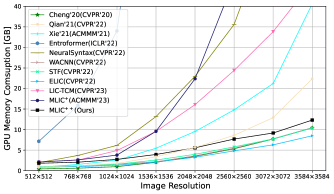
(a)

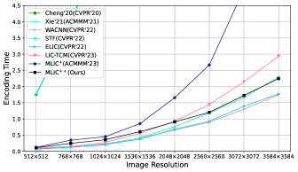
(b)

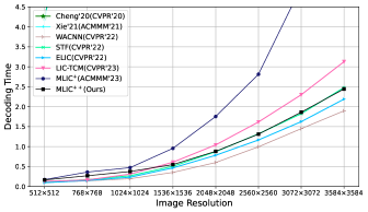
(c)

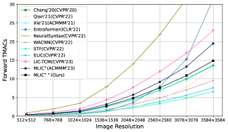
(d)

Figure 12: GPU memory consumption, encoding time, decoding time comparisons among our proposed models (Cheng et al., 2020; Xie et al., 2021; Qian et al., 2022; Zou et al., 2022; He et al., 2022; Liu et al., 2023) and recent learned image compression models. Encoding and decoding time of Qian’21 (Qian et al., 2020), Entroformer (Qian et al., 2022), NeuralSyntax (Wang et al., 2022) exceed 4.5s.

Context Modules	MLIC++	Case 1	Case 2	Case 3	Case 4	Case 5	Case 6	Case 7	Case 8
Channel context module $g_{ch}$	✔	✔	✔	✔	✔	✔	✔	✔	✗
Checkerboard context module $g_{lc,ckbd}$	✗	✗	✗	✗	✗	✗	✔	✗	✗
Checkerboard attention context module $g_{lc,attn}$	✔	✔	✔	✔	✔	✔	✗	✗	✗
Linear intra-slice global spatial context module $g_{gc,intra}$	✔	✔	✗	✔	✔	✗	✗	✗	✗
Linear inter-slice global spatial context module $g_{gc,inter}$	✔	✗	✔	✗	✗	✗	✗	✗	✗
Position embedding	✔	✔	✔	✔	✗	✗	✗	✗	✗
DepthRB	✔	✔	✔	✗	✔	✗	✗	✗	✗
	$0.00$	$+3.15$	$+2.79$	$+4.37$	$+4.10$	$+12.92$	$+15.24$	$+17.45$	$+22.34$

Table 4: Ablation Studies on Kodak. BD-rate (%) is employed to evaluate their contributions. MLIC⁺⁺ is the anchor.

4.4 Computational Complexity

The computational complexity of models is measured in four aspects, including test GPU memory consumption, encoding time, decoding time, and forward Multiply-Accumulate operations (MACs). These metrics provide a comprehensive evaluation of the complexity from various perspectives, with particular emphasis on the first three metrics due to their direct relevance to real-world scenarios. It is worth noting that a model with lower MACs may exhibit slower encoding and decoding speeds if the context module is serial and consume a larger amount of GPU memory. Therefore, while MACs serves as an important measure of complexity, it should be considered in conjunction with the other metrics to obtain a more complete understanding of the characteristics of the model.

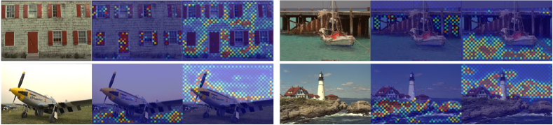
Figure 13: Intra-slice global spatial attention map $\textrm{softmax}_{2}\left(\hat{\boldsymbol{y}}^{i}_{na,q}\right)\left[j\right]\times\textrm{softmax}_{1}\left(\hat{\boldsymbol{y}}^{i}_{ac,k}\right)^{\top}$ of Kodim01, Kodim11, Kodim20, Kodim21 from Kodak (Kodak, 1993) dataset, where $i$ is the index of selected slice, $j$ is the index of selected query. Because interactions within anchor and non-anchor part are not allowed, the attention map is checkerboard-like.

In order to better fit the real-world scenario, we test the model complexities in the case of different resolution images as inputs. We select $16$ images with resolution larger than $3584\times 3584$ from LIU4K test dataset (Liu et al., 2020a) and we center crop these images to $\{512\times 512,768\times 768,1024\times 1024,1536\times 1536,2048\times 2048,2560\times 2560,3072\times 3072,3584\times 3584\}$ patches. We compared our MLIC⁺⁺ with our prior work MLIC⁺ which employs vanilla attention to illustrate the advantages of proposed linear complexity global context capturing. We also compare our proposed MLIC⁺⁺ with recent learned image compression models (Cheng et al., 2020; Qian et al., 2020; Xie et al., 2021; Qian et al., 2022; Wang et al., 2022; Zou et al., 2022; He et al., 2022; Liu et al., 2023). The experiments are conducted on a Tesla A100 GPU and a Xeon(R) Platinum 8260C CPU. The results are illustrated in Fig. 12.

4.4.1 On GPU Memory comsuption

The quadratic complexity of vanilla attention leads to significantly more memory consumptions on high resolution image coding. When compressing $2048\times 2048$ images, MLIC⁺ consumes nearly $22.37$ GB GPU memory. Our proposed linear complexity global context capturing significantly reduces the consumption of GPU memory as our proposed MLIC⁺⁺ only takes about $5.55$ GB GPU memory to compress a $2048\times 2048$ image. When compressing $3072\times 3072$ images, MLIC⁺ consumes $46.38$ GB GPU memory while our proposed MLIC⁺⁺ only consumes $7.69$ GB GPU memory. Compared with recent LIC-TCM (Liu et al., 2023), our MLIC⁺⁺ consumes $\frac{1}{2}$ of the GPU memory consumed by LIC-TCM when compressing $2048\times 2048$ images. When compressing $2560\times 2560$ images, our MLIC⁺⁺ only consumes about $\frac{1}{4}$ of the GPU memory consumed by LIC-TCM. When compressing a $3584\times 3584$ image, the GPU memory consumption of our proposed MLIC⁺⁺ is still only $12.3$ GB while the LIC-TCM requires $45.95$ GB GPU memory. The curve of the GPU memory consumed by our MLIC⁺⁺ as the resolution grows is also much flatter.

4.4.2 On Encoding and Decoding Time

When counting encoding time and decoding time, entropy coding and entropy decoding time are included. Since our MLIC⁺⁺ does not employ pixel-cnn-like spatial context capturing, our MLIC⁺⁺ encodes and decodes much faster than Cheng’20, Xie’21, and Entroformer. The linear complexity global context capturing leads to significant computational overhead reductions on high resolution images when compared with quadratic complexity based global context capturing. Compared with vanilla-attention based method, MLIC⁺⁺ encodes, decodes faster than MLIC⁺ on $\{768\times 768,1024\times 1024,1536\times 1536,2048\times 2048,2560\times 2560\,3072\times 3072,3584\times 3584\}$ images. The time of MLIC⁺⁺ to encode $2560\times 2560$ images is about $\frac{1}{2}$ of the time of MLIC⁺. Compared with recent LIC-TCM, MLIC⁺⁺ needs more time to decode low resolution images while needs less time to encode high-resolution images, which can be attributed to fewer slices in LIC-TCM. At smaller resolutions, the bottleneck of encoding or decoding time is the number of slices, since the encoding and decoding of slices is serial, however, at larger resolutions, the bottleneck is no longer the number of slices but the overall computational complexity due to the high computational overhead of each slice.

4.4.3 On Forward MACs

Compared with MLIC⁺, our MLIC⁺⁺, which employs the proposed linear complexity global spatial context modules, has lower MACs. Compared with the recent LIC-TCM (Liu et al., 2023), our MLIC⁺⁺ demonstrates significantly reduced MACs. Compared with ELIC (He et al., 2022), STF (Zou et al., 2022), and WACNN (Zou et al., 2022), our MLIC⁺⁺ has higher MACs when the input is high-resolution image. One contributing factor to the higher MACs is the utilization of Cheng’20 (Cheng et al., 2020) as the basis for the transform module in our proposed MLIC⁺⁺. While the context module in Cheng’20 is simpler than that of ELIC, STF, and WACNN, the overall MACs of Cheng’20 are higher due to its transform modules having higher MACs. Since our MLIC⁺⁺ employs a modification of analysis transform and synthesis transform of Cheng’20, it results in higher MACs compared to ELIC and WACNN. In addition, since our MLIC⁺⁺ employed an more advanced entropy model, which leads to higher MACs. However, the entropy model has modest effect on the overall MACs since the input image is down-sampled for four times in analysis transform, which implies that designing more advanced entropy models is more resource-efficient.

4.5 Ablation Studies

4.5.1 Settings

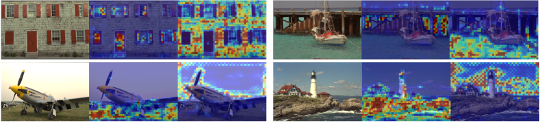
Figure 14: Inter-slice global spatial attention map $\textrm{softmax}_{2}\left(\hat{\boldsymbol{y}}^{i}_{q}\right)\left[j\right]\times\textrm{softmax}_{1}\left(\hat{\boldsymbol{y}}^{i}_{k}\right)^{\top}$ of Kodim01, Kodim11, Kodim20, Kodim21 from Kodak (Kodak, 1993) dataset, where $i$ is the index of selected slice, $j$ is the index of selected query.

We conduct corresponding ablation studies and evaluate the contribution of each module on Kodak (Kodak, 1993) dataset. Each model is optimized for MSE. We train each model for 2M steps. We use the training strategy in Section 4.1.

4.5.2 Analysis of Channel-wise Context Module

The inclusion of a channel-wise context module yields a substantial performance improvement when compared to Case 8, which solely incorporates hyper-priors, Case 7, incorporating channel-wise context modules, achieves a further reduction of $4.89\%$ in bit-rate. The channel-wise context module has the capability to reference symbols in the same and nearby positions in the preceding slices. The effectiveness of the channel-wise context module provides evidence of redundancy among channels.

4.5.3 Analysis of Local Spatial Context Module

The vanilla checkerboard context module leads to slight performance degradation (He et al., 2021) compared with pixel-cnn-like serial context modules (Van den Oord et al., 2016; Minnen et al., 2018). The vanilla checkerboard context module contains one convolutional layer which is linear. The other drawback is the fixed kernel weights during inference. In contrast, our proposed checkerboard attention-based local spatial context module is non-linear and incorporates dynamic attention map generation with two-pass decoding, allowing for improved flexibility and adaptability. Our proposed checkerboard attention-based local spatial context module achieves a further reduction of $2.32\%$ in bit-rate compared to vanilla checkerboard context module. Compared with Case 7, which solely incorporates channel-wise context modules, models incorporating both local spatial and channel context modules demonstrate superior performance, further validating the presence of redundancy in the local spatial domain.

4.5.4 Analysis of Intra-Slice Global Context Module

The $i$-th slice is used as an example to illustrate the process. In practice, the computation of $\textrm{softmax}_{1}\left(\hat{\boldsymbol{y}}^{i-1}_{ac,k}\right)^{\top}\hat{\boldsymbol{y}}^{i}_{ac,v}$ in Equation 15 is performed first for linear complexity. However, we can still compute $\textrm{softmax}_{2}\left(\hat{\boldsymbol{y}}^{i}_{na,q}\right)\left[j\right]\times\textrm{softmax}_{1}\left(\hat{\boldsymbol{y}}^{i}_{ac,k}\right)^{\top}$ as the attention map to validate the ability to capture global dependencies since the $\textrm{softmax}_{2}\left(\hat{\boldsymbol{y}}^{i}_{na,q}\right)\left[j\right]\times\textrm{softmax}_{1}\left(\hat{\boldsymbol{y}}^{i}_{ac,k}\right)^{\top}$ is employed as the implicit similarity metric, where $j$ is the index of selected query. The attention maps of Kodim01, Kodim11, Kodim 20, Kodim21 captured by proposed intra-slice global spatial context module $g_{gc,intra}$ is illustrated in Fig. 13. The checkerboard-like pattern in the attention map arises due to the absence of interactions within the anchor and non-anchor parts. Our model successfully captures distant correlations between the anchor and non-anchor parts, which local context modules are unable to achieve. Although our intra-slice global context module may bear some resemblance to cross-attention models, we focus solely on the interactions within a single slice. We only use the attention map of $\hat{\boldsymbol{y}}^{i-1}$ to predict correlations in $\hat{\boldsymbol{y}}^{i}$. When our proposed global context modules collaborate with local spatial context modules, the overall performance is further improved, underscoring the necessity of global spatial context modules for capturing global correlations and local spatial context modules for capturing local correlations.

4.5.5 Analysis of Inter-Slice Global Context Module

Taken $i$-th slice as an example,in linear complexity inter-slice global context module $g_{gc,inter}$ computes $\textrm{softmax}_{1}\left(\hat{\boldsymbol{y}}^{i}_{k}\right)^{\top}\times\hat{\boldsymbol{y}}^{i}_{v}$ first. However, the $\textrm{softmax}_{2}\left(\hat{\boldsymbol{y}}^{i}_{q}\right)\left[j\right]\times\textrm{softmax}_{1}\left(\hat{\boldsymbol{y}}^{i}_{k}\right)^{\top}$ can be computed as the attention map to validate the ability to capture inter-slice global dependencies, where $j$ is the index of the selected query. The attention maps of Kodim01, Kodim11, Kodim20, Kodim21 captured by our inter-slice are illustrated in Fig. 14. The visualized attention maps clearly demonstrate the effective capture of global dependencies by our $g_{gc,inter}$, despite the model being trained in an implicit manner. When $g_{gc,inter}$ collaborates with the intra-slice global context module $g_{gc,intra}$, teh local spatial context module, and the channel-wise context module, the rate-distortion performance of the model is further enhanced, which demonstrate the effectiveness of inter-slice global context module.

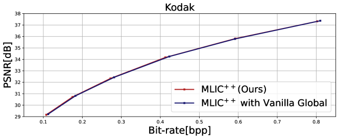
Figure 15: Rate-distortion performance comparisons between MLIC⁺⁺ and MLIC⁺⁺ with vanilla quadratic complexity global spatial context modules.

Patch Size	$256\times 256$	$320\times 320$	$512\times 512$
	$0.00$	$-3.66$	$-6.12$

Table 5: BD-RATE(%) of training using different patch size. The anchor is MLIC⁺⁺ trained on $256\times 256$ patches.

Context Module	$g_{ch}$	$g_{lc,attn}$	$g_{gc,intra}$	$g_{gc,inter}$
KParams	$5810.11$	$755.2$	$732.5$	$4633.34$
MMACs	$8925.18$	$1148.2$	$1116.2$	$7100.50$

Table 6: Parameters and Forward Macs of context modules on Kodak.

4.5.6 Analysis on Learnable Position Embedding and DepthRB

The position embedding and DepthRB lead to performance gains as illustrated in Table 4. Specifically, when DepthRB is not employed, a FFN is utilized instead. The learnable position embedding is flexible because it is data-driven. Other position embedding method, Sinusoidal Position Embedding (Vaswani et al., 2017), is tried and it leads negligible performance difference compared to model without position embedding. Relative Position Embedding (Shaw et al., 2018) is employed on attention map, which cannot be employed in our approach because the $\textrm{softmax}_{1}\left(\hat{\boldsymbol{y}}^{i-1}_{ac,k}\right)^{\top}\hat{\boldsymbol{y}}^{i}_{ac,v}$ and $\textrm{softmax}_{1}\left(\hat{\boldsymbol{y}}^{<i}_{k}\right)^{\top}\hat{\boldsymbol{y}}^{<i}_{v}$ are computed first in our approach for linear complexity instead of the attention map $\textrm{softmax}_{2}\left(\hat{\boldsymbol{y}}^{i}_{na,q}\right)\left[j\right]\times\textrm{softmax}_{1}\left(\hat{\boldsymbol{y}}^{i}_{ac,k}\right)^{\top}$ and $\textrm{softmax}_{2}\left(\hat{\boldsymbol{y}}^{i}_{q}\right)\left[j\right]\times\textrm{softmax}_{1}\left(\hat{\boldsymbol{y}}^{i}_{k}\right)^{\top}$. The learnable position embedding is not employed in our checkerboard attention-based local spatial context module $g_{lc,attn}$, because the performance improvement is quite negligible. In our $g_{lc,attn}$, the feature is partition into overlapped windows with zero padding. The zero padding and boundary effects imply that there is no need to insert a position embedding layer.

4.5.7 Comparisons with Model with Vanilla Global Spatial Context Modules

The comparison between MLIC⁺⁺ and MLIC⁺⁺ with vanilla quadratic complexity global spatial context modules is illustrated in Fig. 15. It is evident that modeling global spatial contexts using linear complexity attention mechanisms does not result in performance degradation when compared to the vanilla attention mechanism.

4.5.8 Analysis of Training with Large Patches

In our training strategy, we use $512\times 512$ patches to train MLIC⁺⁺ during the rest $0.8$M steps. We compare the differences in rate-distortion performance between different patch sizes $\{256\times 256,320\times 320,512\times 512\}$ during the rest $0.8$M steps in Table 5. Using large patches further boost the model performance. Using $256\times 256$ patches cannot fully exploit the performance of the model. The size of latent representation is $16\times 16$ if $256\times 256$ patches are adopted. $16\times 16$ latent representation is insufficient for model to learn long-range or global dependency as the resolutions of input images of the codec could be 2K or 4K. Moreover, checkerboard partition (He et al., 2021) is employed, which makes the attention map sparse. Therefore, it is required to adopt large patches for better performance. Considering the overhead of training and model performance, adopting $512\times 512$ patches is the best choice.

4.5.9 Comparisons among Different Context Modules

As illustrated in Table 4, the proposed global context modules $g_{gc,intra}$ and $g_{gc,inter}$ contribute most to performance, channel-wise context module $g_{ch}$ has the second highest contribution to performance, and local sptail context module $g_{lc,attn}$ has the lowest contribution to performance. Since each context module has a different role to perform, it is imperative that they work together for performance enhancement. The complexity of each context module is presented in Table 6. The channel-wise context module has the most parameters and highest MACs. However, the MACs of the channel context module are only $1.77\%$ of the total MACs. The total MACs of all context modules are only $3.63\%$ of the total MACs.

5 Conclusion

In this paper, we propose a novel approach for capturing local spatial context using checkerboard attention, as well as linear complexity intra-slice and inter-slice global context modules, which significantly enhance the performance of the model while maintaining an acceptable linear complexity. Based on proposed context modules, we propose linear complexity multi-reference entropy model MEM⁺⁺. Building upon MEM⁺⁺, we obtain state-of-the-art model MLIC⁺⁺. MLIC⁺⁺ exhibits linear GPU memory consumption with resolution, making it highly suitable for high-resolution image coding. To make our MLIC⁺⁺ more practical, our future work will focus on investigating the asymmetrical design (Yang & Mandt, 2023) between the analysis and synthesis transforms, as well as lighter linear complexity multi-reference entropy model.

References

- Agustsson & Timofte (2017) Agustsson, E. and Timofte, R. Ntire 2017 challenge on single image super-resolution: Dataset and study. 2017 IEEE Conference on Computer Vision and Pattern Recognition Workshops, pp. 1122–1131, 2017.
- Asuni & Giachetti (2014) Asuni, N. and Giachetti, A. Testimages: a large-scale archive for testing visual devices and basic image processing algorithms. In STAG: Smart Tools & Apps for Graphics (2014), 2014.
- Ballé et al. (2015) Ballé, J., Laparra, V., and Simoncelli, E. P. Density modeling of images using a generalized normalization transformation. arXiv preprint arXiv:1511.06281, 2015.
- Ballé et al. (2017) Ballé, J., Laparra, V., and Simoncelli, E. P. End-to-end optimized image compression. In International Conference on Learning Representations, 2017.
- Ballé et al. (2018) Ballé, J., Minnen, D., Singh, S., Hwang, S. J., and Johnston, N. Variational image compression with a scale hyperprior. In International Conference on Learning Representations, 2018.
- Bégaint et al. (2020) Bégaint, J., Racapé, F., Feltman, S., and Pushparaja, A. Compressai: a pytorch library and evaluation platform for end-to-end compression research. arXiv preprint arXiv:2011.03029, 2020.
- Bjontegaard (2001) Bjontegaard, G. Calculation of average psnr differences between rd-curves. ITU SG16 Doc. VCEG-M33, 2001.
- Bross et al. (2021) Bross, B., Wang, Y.-K., Ye, Y., Liu, S., Chen, J., Sullivan, G. J., and Ohm, J.-R. Overview of the versatile video coding (vvc) standard and its applications. IEEE Transactions on Circuits and Systems for Video Technology, 31(10):3736–3764, 2021.
- Charrier et al. (1999) Charrier, M., Cruz, D. S., and Larsson, M. Jpeg2000, the next millennium compression standard for still images. In IEEE International Conference on Multimedia Computing and Systems, ICMCS, pp. 131–132. IEEE Computer Society, 1999.
- Chen et al. (2022) Chen, F., Xu, Y., and Wang, L. Two-stage octave residual network for end-to-end image compression. In Proceedings of the AAAI Conference on Artificial Intelligence, volume 36, pp. 3922–3929, 2022.
- Chen & Ma (2023) Chen, T. and Ma, Z. Toward robust neural image compression: Adversarial attack and model finetuning. IEEE Transactions on Circuits and Systems for Video Technology, 33(12):7842–7856, 2023.
- Chen et al. (2021) Chen, T., Liu, H., Ma, Z., Shen, Q., Cao, X., and Wang, Y. End-to-end learnt image compression via non-local attention optimization and improved context modeling. IEEE Transactions on Image Processing, 30:3179–3191, 2021.
- Cheng et al. (2020) Cheng, Z., Sun, H., Takeuchi, M., and Katto, J. Learned image compression with discretized gaussian mixture likelihoods and attention modules. In Proceedings of the IEEE/CVF Conference on Computer Vision and Pattern Recognition, June 2020.
- Cui et al. (2021) Cui, Z., Wang, J., Gao, S., Guo, T., Feng, Y., and Bai, B. Asymmetric gained deep image compression with continuous rate adaptation. In Proceedings of the IEEE/CVF Conference on Computer Vision and Pattern Recognition, pp. 10532–10541, June 2021.
- Deng et al. (2009) Deng, J., Dong, W., Socher, R., Li, L.-J., Li, K., and Fei-Fei, L. Imagenet: A large-scale hierarchical image database. In 2009 IEEE conference on computer vision and pattern recognition, pp. 248–255. Ieee, 2009.
- Dosovitskiy et al. (2021) Dosovitskiy, A., Beyer, L., Kolesnikov, A., Weissenborn, D., Zhai, X., Unterthiner, T., Dehghani, M., Minderer, M., Heigold, G., Gelly, S., et al. An image is worth 16x16 words: Transformers for image recognition at scale. In International Conference on Learning Representations, 2021.
- Duan et al. (2023) Duan, Z., Lu, M., Ma, Z., and Zhu, F. Lossy image compression with quantized hierarchical vaes. In Proceedings of the IEEE/CVF Winter Conference on Applications of Computer Vision, pp. 198–207, 2023.
- Feng et al. (2023) Feng, R., Guo, Z., Li, W., and Chen, Z. Nvtc: Nonlinear vector transform coding. In Proceedings of the IEEE/CVF Conference on Computer Vision and Pattern Recognition, pp. 6101–6110, June 2023.
- Fu et al. (2023a) Fu, H., Liang, F., Liang, J., Li, B., Zhang, G., and Han, J. Asymmetric learned image compression with multi-scale residual block, importance scaling, and post-quantization filtering. IEEE Transactions on Circuits and Systems for Video Technology, 33(8):4309–4321, 2023a. doi: 10.1109/TCSVT.2023.3237274.
- Fu et al. (2023b) Fu, H., Liang, F., Lin, J., Li, B., Akbari, M., Liang, J., Zhang, G., Liu, D., Tu, C., and Han, J. Learned image compression with gaussian-laplacian-logistic mixture model and concatenated residual modules. IEEE Transactions on Image Processing, 32:2063–2076, 2023b.
- Gao et al. (2021) Gao, G., You, P., Pan, R., Han, S., Zhang, Y., Dai, Y., and Lee, H. Neural image compression via attentional multi-scale back projection and frequency decomposition. In Proceedings of the IEEE/CVF International Conference on Computer Vision, pp. 14677–14686, 2021.
- Guo et al. (2022) Guo, Z., Zhang, Z., Feng, R., and Chen, Z. Causal contextual prediction for learned image compression. IEEE Transactions on Circuits and Systems for Video Technology, 32(4):2329–2341, 2022.
- He et al. (2021) He, D., Zheng, Y., Sun, B., Wang, Y., and Qin, H. Checkerboard context model for efficient learned image compression. In Proceedings of the IEEE/CVF Conference on Computer Vision and Pattern Recognition, pp. 14771–14780, 2021.
- He et al. (2022) He, D., Yang, Z., Peng, W., Ma, R., Qin, H., and Wang, Y. Elic: Efficient learned image compression with unevenly grouped space-channel contextual adaptive coding. In Proceedings of the IEEE/CVF Conference on Computer Vision and Pattern Recognition, June 2022.
- Hu et al. (2020) Hu, Y., Yang, W., and Liu, J. Coarse-to-fine hyper-prior modeling for learned image compression. In Proceedings of the AAAI Conference on Artificial Intelligence, volume 34, pp. 11013–11020, 2020.
- Islam et al. (2019) Islam, M. A., Jia, S., and Bruce, N. D. How much position information do convolutional neural networks encode? In International Conference on Learning Representations, 2019.
- Jiang et al. (2023a) Jiang, W., Ning, P., and Wang, R. Slic: Self-conditioned adaptive transform with large-scale receptive fields for learned image compression. arXiv preprint arXiv:2304.09571, 2023a.
- Jiang et al. (2023b) Jiang, W., Yang, J., Zhai, Y., Ning, P., Gao, F., and Wang, R. Mlic: Multi-reference entropy model for learned image compression. In Proceedings of the 31st ACM International Conference on Multimedia, 2023b. doi: 10.1145/3581783.3611694.
- Kayhan & Gemert (2020) Kayhan, O. S. and Gemert, J. C. v. On translation invariance in cnns: Convolutional layers can exploit absolute spatial location. In Proceedings of the IEEE/CVF Conference on Computer Vision and Pattern Recognition, pp. 14274–14285, 2020.
- Kim et al. (2022) Kim, J.-H., Heo, B., and Lee, J.-S. Joint global and local hierarchical priors for learned image compression. In Proceedings of the IEEE/CVF Conference on Computer Vision and Pattern Recognition, 2022.
- Kingma & Welling (2014) Kingma, D. P. and Welling, M. Auto-encoding variational bayes. In International Conference on Learning Representations, 2014.
- Kodak (1993) Kodak, E. Kodak lossless true color image suite, 1993.
- Koyuncu et al. (2022) Koyuncu, A. B., Gao, H., Boev, A., Gaikov, G., Alshina, E., and Steinbach, E. Contextformer: A transformer with spatio-channel attention for context modeling in learned image compression. In European Conference on Computer Vision, pp. 447–463, 2022.
- Lim et al. (2017) Lim, B., Son, S., Kim, H., Nah, S., and Mu Lee, K. Enhanced deep residual networks for single image super-resolution. In Proceedings of the IEEE conference on computer vision and pattern recognition workshops, 2017.
- Lin et al. (2014) Lin, T.-Y., Maire, M., Belongie, S., Hays, J., Perona, P., Ramanan, D., Dollár, P., and Zitnick, C. L. Microsoft coco: Common objects in context. In European Conference on Computer Vision, pp. 740–755, 2014.
- Liu et al. (2020a) Liu, J., Liu, D., Yang, W., Xia, S., Zhang, X., and Dai, Y. A comprehensive benchmark for single image compression artifact reduction. IEEE Transactions on image processing, 29:7845–7860, 2020a.
- Liu et al. (2020b) Liu, J., Lu, G., Hu, Z., and Xu, D. A unified end-to-end framework for efficient deep image compression. arXiv preprint arXiv:2002.03370, 2020b.
- Liu et al. (2023) Liu, J., Sun, H., and Katto, J. Learned image compression with mixed transformer-cnn architectures. In Proceedings of the IEEE/CVF Conference on Computer Vision and Pattern Recognition, 2023.
- Liu et al. (2021) Liu, Z., Lin, Y., Cao, Y., Hu, H., Wei, Y., Zhang, Z., Lin, S., and Guo, B. Swin transformer: Hierarchical vision transformer using shifted windows. In Proceedings of the IEEE/CVF International Conference on Computer Vision (ICCV), pp. 10012–10022, October 2021.
- Lu et al. (2022) Lu, M., Guo, P., Shi, H., Cao, C., and Ma, Z. Transformer-based image compression. In Data Compression Conference, pp. 469–469, 2022.
- Ma et al. (2021) Ma, C., Wang, Z., Liao, R., and Ye, Y. A cross channel context model for latents in deep image compression. arXiv preprint arXiv:2103.02884, 2021.
- Ma et al. (2020) Ma, H., Liu, D., Yan, N., Li, H., and Wu, F. End-to-end optimized versatile image compression with wavelet-like transform. IEEE Transactions on Pattern Analysis and Machine Intelligence, 2020.
- Minnen & Singh (2020) Minnen, D. and Singh, S. Channel-wise autoregressive entropy models for learned image compression. In 2020 IEEE International Conference on Image Processing (ICIP), pp. 3339–3343. IEEE, 2020.
- Minnen et al. (2018) Minnen, D., Ballé, J., and Toderici, G. D. Joint autoregressive and hierarchical priors for learned image compression. In Advances in Neural Information Processing Systems, pp. 10771–10780, 2018.
- Pan et al. (2022) Pan, G., Lu, G., Hu, Z., and Xu, D. Content adaptive latents and decoder for neural image compression. In European Conference on Computer Vision, pp. 556–573, 2022.
- Paszke et al. (2019) Paszke, A., Gross, S., Massa, F., Lerer, A., Bradbury, J., Chanan, G., Killeen, T., Lin, Z., Gimelshein, N., Antiga, L., et al. Pytorch: An imperative style, high-performance deep learning library. In Advances in Neural Information Processing Systems, pp. 8024–8035, 2019.
- Pennebaker & Mitchell (1992) Pennebaker, W. B. and Mitchell, J. L. JPEG: Still image data compression standard. Springer Science & Business Media, 1992.
- Qian et al. (2020) Qian, Y., Tan, Z., Sun, X., Lin, M., Li, D., Sun, Z., Hao, L., and Jin, R. Learning accurate entropy model with global reference for image compression. In International Conference on Learning Representations, 2020.
- Qian et al. (2022) Qian, Y., Lin, M., Sun, X., Tan, Z., and Jin, R. Entroformer: A transformer-based entropy model for learned image compression. In International Conference on Learning Representations, 2022.
- Shaw et al. (2018) Shaw, P., Uszkoreit, J., and Vaswani, A. Self-attention with relative position representations. arXiv preprint arXiv:1803.02155, 2018.
- Shen et al. (2021) Shen, Z., Zhang, M., Zhao, H., Yi, S., and Li, H. Efficient attention: Attention with linear complexities. In Proceedings of the IEEE/CVF Winter Conference on Applications of Computer Vision, 2021.
- Sullivan et al. (2012) Sullivan, G. J., Ohm, J.-R., Han, W.-J., and Wiegand, T. Overview of the high efficiency video coding (hevc) standard. IEEE Transactions on circuits and systems for video technology, 22(12):1649–1668, 2012.
- Tang et al. (2023) Tang, Z., Wang, H., Yi, X., Zhang, Y., Kwong, S., and Kuo, C.-C. J. Joint graph attention and asymmetric convolutional neural network for deep image compression. IEEE Transactions on Circuits and Systems for Video Technology, 33(1):421–433, 2023. doi: 10.1109/TCSVT.2022.3199472.
- Theis et al. (2017) Theis, L., Shi, W., Cunningham, A., and Huszár, F. Lossy image compression with compressive autoencoders. In International Conference on Learning Representations, 2017.
- Toderici et al. (2020) Toderici, G., Shi, W., Timofte, R., Theis, L., Ballé, J., Agustsson, E., Johnston, N., and Mentzer, F. Workshop and challenge on learned image compression (clic2020), 2020.
- Van den Oord et al. (2016) Van den Oord, A., Kalchbrenner, N., Espeholt, L., Vinyals, O., Graves, A., et al. Conditional image generation with pixelcnn decoders. Advances in neural information processing systems, 29, 2016.
- Vaswani et al. (2017) Vaswani, A., Shazeer, N., Parmar, N., Uszkoreit, J., Jones, L., Gomez, A. N., Kaiser, Ł., and Polosukhin, I. Attention is all you need. Advances in neural information processing systems, 30:5998–6008, 2017.
- Wang et al. (2022) Wang, D., Yang, W., Hu, Y., and Liu, J. Neural data-dependent transform for learned image compression. In Proceedings of the IEEE/CVF Conference on Computer Vision and Pattern Recognition, 2022.
- Wang et al. (2021) Wang, Y., Liu, D., Ma, S., Wu, F., and Gao, W. Ensemble learning-based rate-distortion optimization for end-to-end image compression. IEEE Transactions on Circuits and Systems for Video Technology, 31(3):1193–1207, 2021.
- Wang et al. (2003) Wang, Z., Simoncelli, E. P., and Bovik, A. C. Multiscale structural similarity for image quality assessment. In The Thrity-Seventh Asilomar Conference on Signals, Systems & Computers, 2003, volume 2. Ieee, 2003.
- Wiegand et al. (2003) Wiegand, T., Sullivan, G., Bjontegaard, G., and Luthra, A. Overview of the h.264/avc video coding standard. IEEE Transactions on Circuits and Systems for Video Technology, 13(7):560–576, 2003. doi: 10.1109/TCSVT.2003.815165.
- Wu et al. (2022) Wu, Y., Li, X., Zhang, Z., Jin, X., and Chen, Z. Learned block-based hybrid image compression. IEEE Transactions on Circuits and Systems for Video Technology, 32(6):3978–3990, 2022.
- Xie et al. (2021) Xie, Y., Cheng, K. L., and Chen, Q. Enhanced invertible encoding for learned image compression. In Proceedings of the ACM International Conference on Multimedia, pp. 162–170, 2021.
- Yang & Mandt (2023) Yang, Y. and Mandt, S. Computationally-efficient neural image compression with shallow decoders. In Proceedings of the IEEE/CVF International Conference on Computer Vision (ICCV), pp. 530–540, 2023.
- Zhu et al. (2022a) Zhu, X., Song, J., Gao, L., Zheng, F., and Shen, H. T. Unified multivariate gaussian mixture for efficient neural image compression. In Proceedings of the IEEE/CVF Conference on Computer Vision and Pattern Recognition, pp. 17612–17621, 2022a.
- Zhu et al. (2022b) Zhu, Y., Yang, Y., and Cohen, T. Transformer-based transform coding. In International Conference on Learning Representations, 2022b.
- Zou et al. (2022) Zou, R., Song, C., and Zhang, Z. The devil is in the details: Window-based attention for image compression. In In Proceedings of the IEEE conference on computer vision and pattern recognition, 2022.